
Submitted:
03 July 2025
Posted:
03 July 2025
You are already at the latest version
Abstract
Functional-order (variable-order) fractional diffusion–wave equations introduce considerable computational challenges, as the fractional order of the derivatives can vary spatially or temporally. To overcome these challenges, a novel spectral method employing generalized fractional-order Chelyshkov wavelets is developed to efficiently solve such equations. In this approach, the Riemann–Liouville fractional integral operator of variable order is evaluated in closed form via a regularized incomplete Beta function, enabling the transformation of the governing equation into a symmetric system of algebraic equations. This wavelet-based spectral scheme attains extremely high accuracy, yielding significantly lower errors than existing numerical techniques. Its strong convergence properties allow high precision to be achieved with relatively few wavelet basis functions, leading to efficient computations. The method’s accuracy and efficiency are demonstrated on several practical diffusion–wave examples, indicating its suitability for real-world applications. Furthermore, it readily applies to a wide class of fractional partial differential equations (FPDEs) with spatially or temporally varying order, demonstrating versatility for diverse applications.
Keywords:
fractional-order
; functional-order
; diffusion-wave equation
; Chelyshkov wavelet
; regularized incomplete Beta function.
1. Introduction
Unlike the classical derivative, the use of fractional derivatives in many real-world phenomena can help to capture information of the current state from all its previous states. With this non-local property, fractional differential equations (FDEs) are used in many practical problems, such as modeling heat transfer [1], earthquakes [2], physics and mechanics [3,4,5], chemistry and dynamics in biological tissues [6], engineering [7], control theory [8,9,10], and option pricing [11].
In recent decades, FDEs have been extended to variable-order FDEs (VFDEs). In this equation, the orders of the derivatives can be non-constant functions [12,13,14]. This generalization enhances the fractional derivative’s ability to capture non-local effects, thus, popularizes the applications of VFDEs (see [15] and references therein). The advantages of VFDEs in comparison with FDEs have been discussed in [16], while some results on the consistency of this kind of equation and the uniqueness of the analytical solutions of VFDEs have been given in [17,18,19]. The VFDEs occurring in the applications usually do not have a solution which can be expressed via elementary functions. Therefore, it is crucial to design efficient methods for approximating solutions of VFDEs. The available methods can be seen in [20,21,22,23].
Recently, wavelets have become an important tool for solving fractional calculus problems. For example, Legendre wavelets have been used efficiently in various methods [24]. Chebyshev wavelets demonstrated high accuracy in many methods [25,26]. Some other useful wavelets are the Bernoulli and Taylor wavelets [27,28].
In [29] and [30], fractional-order Laguerre and Legendre functions are introduced to improve the accuracy of solutions for FDEs that contain power terms of fractional-order. In addition, generalized Legendre and Bernoulli wavelets were given in [31] and [32]. In these methods, finding the Riemann-Liouville integral operator with functional-order(RLI-FO) of the bases was an important step. The RLI-FO of hybrid Bernoulli polynomials was derived in [33,34] by using Laplace transforms. The same argument was used for Taylor wavelets in [28,35]. However, the Laplace transform cannot be used to find the closed form formula for the RLI-FO of any generalized form in both cases of polynomials and wavelets.
In this article, we provide a numerical technique for the solution of FO-FDWEs given in [36] by
where ; are constants; ; and are known functions. Here, and denote the Caputo functional-order derivative (CFD) defined by
In the current paper, we numerically solve the FO-FDWE given in Eqs. (1)-(3) by using FOCW. The FOCW technique provides several benefits, including the orthogonality and the spectral accuracy properties [37,38]. The regularized incomplete Beta functions are used to derive an exact value for the RLI-FO of order for the FOCW. This exact value can be used to simplify Eqs. (1)-(3) into a system of algebraic equations. In general, this system can be computationally complex and require a large storage space for large systems. However, by using FOCW, the computational complexity can be reduced [39]. The structure of this article is arranged as follows. The RLI-FO, the CFD, and the regularized incomplete Beta functions are recalled in Section 2. In Section 3, we construct the FOCW and find the exact value of their RLI-FO by using the regularized incomplete Beta functions. In Section 4 and Section 5, we present the idea of the method and its error estimation. In Section 6, several examples are included. In addition, in Example 1, we will get the exact solution which was not obtained in [36]. In example2,example3,ex7, we will point out that we will obtain better solutions than other methods in the literature.
2. Preliminaries
This section presents the fundamental concepts of the RLI-FO and CFD, which serve as the theoretical basis for our numerical approach. Unless otherwise stated, we assume for all .
Definition 1.
The CFD and the RLI-FO are linear operators. Moreover, we have
- (i)
- For , we have
- (ii)
- For ,
By using the regularized incomplete Beta functions, we get the following lemma:
Lemma 1.
Let , we have
where
3. Fractional-Order Chelyshkov Wavelets and Function Approximations in Two Dimensional Space
The Chelyshkov polynomials are defined as
where
Let be nonnegative integers. The Chelyshkov wavelets for and are defined on as
The FOCW are obtained by using the transformation for some , as
The FOCW form an orthonormal basis for , i.e.
where is the weight function. Therefore a function can be expressed as
where
and
The theorem below establishes a closed-form expression for the variable-order Riemann–Liouville integral of fractional-order Chelyshkov wavelets. This result serves as the foundation for constructing a novel numerical scheme for solving variable-order fractional diffusion–wave equations in the subsequent section.
Theorem 1.
Let , we have
where
and are two parameters defined by
Proof.
First, we reformulate the FOCW in the following form:
Then
After that, we apply Lemma 1 to obtain
If then . In case , then
For , we have
The theorem is then proved. □
In the two-dimensional case, for , and non-negative integers the set
forms an orthonormal set in . Here, the norm is defined by
where and . To create a new arrangement, let and , where , then the orthonormal set becomes
where . Any function can be represented by
where and are given as
and is an matrix with
4. Error Bound
Theorem 2.
Let and let be a smooth function. Suppose that is the best approximation of p out of
with respect to the norm in . Then
where are constants satisfying
Proof.
We denote and . Suppose that the polynomial interpolates the function at the points , where s and are the roots of the Chebyshev polynomial of -degree in and -degree in correspondingly.
Thus
Similar to the methods in References [36,42] and [43,44], we have
where . So we obtain
Since is a smooth function on the compact domain , then there exist satisfying
To evaluate , we consider the mapping
where , and between the intervals and , we get
where are the solutions of the Chebyshev polynomial of degree .
5. Numerical Method
We use FOCW to establish a numerical method for solving the Eq. (1) associated with the conditions (2) and (3). First, we approximate
where are given in Eqs. (7) and (8). By integrating both sides of the above equation with respect to t twice and applying the Eq. (2)
Integrating both sides of Eq. (15) with respect to twice and using the conditions (3) we get
where
and
Therefore
and
where
and are given in Eq. (5). From Eq. (16) we obtain
By substituting Eqs. (15)-(19) in Eq. (1), we get an algebraic equation. By collocating at nodes given by
we can find the unknowns .
6. Illustrative Examples
We compare the experimental results obtained by using our method and with known methods, such as shifted Chebyshev cardinal functions [42], Chebyshev wavelets [36], and generalized polynomials [45] in the following examples:
Example 1
(See [36, Example 1]). Consider the following FO-FDWE:
where ,
and the conditions in Eqs. (2) and (3) are given so that
This example was considered in [36] with . Here, we applied our method with . First, we evaluate
where
and
From Eqs. (15) and (16) we obtain the following.
where
By using Eqs. (17) and (18) we get
and
where
and
From Eq. (19) we get
where
By substituting Eqs. (21) and (23)-(25) in Eq. (20) and collocating the resulted equation at the nodes
we obtain a system of 36 algebraic equations in 36 unknowns . The solution of the system is
By substituting this solution into Eq. (22), we get the exact solution . This solution was not obtained in [36].
In case , by using the same argument as above with , we obtain
which yields the exact solution . This exact solution cannot be obtained by using integer-order polynomial wavelets.
Example 2
(See [36, Example 2]). Consider
where
, , , and . The conditions in Eqs. (2) and (3) are given such that .
First, we solve this problem with . Table 1 presents the maximum of the relative errors (REs) in various pairs of fractional orders , and the minimal of these errors is reached at . In Table 2, we compare the REs for this method with those in [36]. The comparison is based on the same number of elements in the bases of the function approximation. The table suggests that the present method provides approximate solutions with lower error. In Table 2, M is the degree of Chebyshev polynomials. Figure 1 illustrates the graphs of the approximated solution and the absolute error function (AEF) for .
Example 3
(See [36, Example 3]). Consider the nonlinear FO-FDWE
where
and . The conditions in Eqs. (2) and (3) are given such that .
Table 3 provides the maximal AEs of the approximated solutions using our method in the case and various pairs of fractional orders . The table shows that the minimum occurred at . Figure 2 shows the graph of the solution and AEF in cases and . Table 4 and Table 5 compare the REs of numerical solutions using our method with the method in [36] with different values of . These tables indicate that the present method yields more accurate solutions with fewer errors.
Example 4.
In particle physics, anomalous diffusion processes were formulated in terms of diffusion equations by using fractional derivatives and distributed-order derivatives in [46]. As a generalization, we consider the following diffusion equation with variable-order derivative:
where , is the pdf (probability density function) of the diffusion-process, and ν is the diffusion-coefficient of physical dimension (cm2/sec). Following [46], we consider this diffusion equation:
We scale the problem to finite intervals by setting:
Then and Eqs. (26), (27), (28) become
where
7. Conclusions
This study introduced a spectral wavelet-based approach utilizing generalized fractional-order
Chelyshkov wavelets to solve functional-order fractional diffusion–wave equations. The method
demonstrated high computational efficiency and superior accuracy, achieving significantly lower
numerical errors than conventional schemes in benchmark comparisons. The integration of regularized
incomplete Beta functions allowed for an exact representation of the fractional integral operator,
contributing to the stability and effectiveness of the proposed framework. Notably, the method
successfully captured the physical behavior in Example 4, illustrating its capability to handle realworld
models with high fidelity. Given its flexibility and precision, the proposed strategy offers
a promising foundation for solving a broader class of fractional partial differential equations with
variable orders. Future work may extend this framework to diverse applications in physics and
engineering where memory effects and anomalous diffusion are prominent.
References
- Sierociuk, D.; Dzieliński, A.; Sarwas, G.; Petras, I.; Podlubny, I.; Skovranek, T. Modelling heat transfer in heterogeneous media using fractional calculus. Philosophical Transactions of the Royal Society A: Mathematical, Physical and Engineering Sciences 2013, 371, 20120146. [Google Scholar] [CrossRef] [PubMed]
- Lopes, A.M.; Machado, J.A.T.; Pinto, C.M.A.; Galhano, A.M.S.F. Fractional dynamics and mds visualization of earthquake phenomena. Comput. Math. Appl. 2013, 66, 647–658. [Google Scholar] [CrossRef]
- Carpinteri, A.; Mainardi, F. Fractals and fractional calculus in continuum mechanics; Springer, 2014; vol. 378. [Google Scholar]
- Liu, J.; Li, X.; Hu, X. A rbf-based differential quadrature method for solving two-dimensional variable-order time fractional advection-diffusion equation. J. Comput. Phys. 2019, 384, 222–238. [Google Scholar] [CrossRef]
- Rudolf, H. Applications of fractional calculus in physics; World scientific, 2000. [Google Scholar]
- Magin, R.L. Fractional calculus models of complex dynamics in biological tissues. Comput. Math. Appl. 2010, 59, 1586–1593. [Google Scholar] [CrossRef]
- Loverro, A. Fractional calculus: history, definitions and applications for the engineer.Rapport technique, Univeristy of Notre Dame: Department of Aerospace and Mechanical Engineering (2014) 1–28.
- Bock, H.G.; Plitt, K.J. A multiple shooting algorithm for direct solution of optimal control problems. IFAC Proceedings Volumes 1984, 17, 1603–1608. [Google Scholar] [CrossRef]
- Baleanu, D.; Machado, J.A.T.; Luo, A.C.J. Fractional dynamics and control; Springer Science & Business Media, 2011. [Google Scholar]
- Vinagre, B.M.; Feliu, V. Modeling and control of dynamic system using fractional calculus: Application to electrochemical processes and flexible structures. Proc. 41st IEEE Conf. Decision and Control, Las Vegas, NV, 2002; pp. 214–239. [Google Scholar]
- Ghafouri, H.; Ranjbar, M.; Khani, A. The use of partial fractional form of a-stable padé schemes for the solution of fractional diffusion equation with application in option pricing. Comput. Econ. 2019, 1–15. [Google Scholar] [CrossRef]
- Alkahtani, B.S.T.; Koca, I.; Atangan, A. A novel approach of variable order derivative: Theory and methods. J. Nonlinear Sci Appl. 9. 2016. [Google Scholar] [CrossRef]
- Odzijewicz, T.; Malinowska, A.B.; Torres, D.F.M. Fractional variational calculus of variable order. In Advances in harmonic analysis and operator theory; Springer, 2013; pp. 291–301. [Google Scholar]
- Zaky, M.A.; Doha, E.H.; Taha, T.M. Baleanu,D. New recursive approximations for variable-order fractional operators with applications. arXiv 2018, arXiv:1804.01198 2018. [Google Scholar]
- Sun, H.G.; Chang, A.; Zhang, Y.; Chen, W. A review on variable-order fractional differential equations: mathematical foundations, physical models, numerical methods and applications. Fract. Calc. Appl. Anal. 2019, 22, 27–59. [Google Scholar] [CrossRef]
- Sun, H.G.; Chen, W.; Wei, H.; Chen, Y.Q. A comparative study of constant-order and variable-order fractional models in characterizing memory property of systems. Eur. Phys. J. Spec. Top. 2011, 185–192. [Google Scholar] [CrossRef]
- Razminia, R.; Dizaji, A.; Majd, V.J. Solution existence for non-autonomous variable-order fractional differential equations. Math. Comput. Modell. 2011, 55, 1106–1117. [Google Scholar] [CrossRef]
- Zhang, S. Existence and uniqueness result of solutions to initial value problems of fractional differential equations of variable-order. J. Frac. Calc. Anal. 2013, 1, 82–98. [Google Scholar]
- Zhang, S. Existence result of solutions to differential equations of variable-order with nonlinear boundary value conditions. Commun. Nonlinear Sci. Numer. Simul. 2013, 18, 3289–3297. [Google Scholar] [CrossRef]
- Chen, Y.M.; Wei, Y.Q.; Liu, D.Y.; Yu, H. Numerical solution for a class of nonlinear variable order fractional differential equations with legendre wavelets. Appl. Math. Lett. 2015, 83–88. [Google Scholar] [CrossRef]
- Sheng, H.; Sun, H.G.; Coopmans, C.; Chen, Y.Q. ; Bohannan,G.W. A physical experimental study of variable-order fractional integrator and differentiator. Eur. Phys. J. Spec. Top. 2011, 193, 93–104. [Google Scholar] [CrossRef]
- Sun, H.G.; Chen, W.; Chen, Y.Q. Variable-order fractional differential operators in anomalous diffusion modeling. Physica A: Stat. Mecha. Appl. 2009, 388, 4586–4592. [Google Scholar] [CrossRef]
- Usman, M.; Hamid, M.; Haq, R.U.l.; Wang, W. An efficient algorithm based on gegenbauer wavelets for the solutions of variable-order fractional differential equations, Eur. Phys. J. Plus 2018, 133, 327. [Google Scholar] [CrossRef]
- Rawashdeh, E.A. Legendre wavelets method for fractional integro-differential equations. Appl. Math. Sci. 2011, 5, 2467–2474. [Google Scholar]
- Wang, Y.; Fan, Q. The second kind chebyshev wavelet method for solving fractional differential equations. Appl. Math. Comput. 2012, 218, 8592–8601. [Google Scholar] [CrossRef]
- Yuanlu, L. Solving a nonlinear fractional differential equation using chebyshev wavelets. Commun. Nonlinear Sci. Numer. Simul. 2010, 15, 2284–2292. [Google Scholar]
- Keshavarz, E.; Ordokhani, Y.; Razzaghi, M. Bernoulli wavelet operational matrix of fractional order integration and its applications in solving the fractional order differential equations. Applied Mathematical Modelling 2014, 38, 6038–6051. [Google Scholar] [CrossRef]
- Phan, T.T.; Vo, N.T.; Razzaghi, M. Taylor wavelet method for fractional delay differential equations. Eng. Comput. 2021, 37, 231–240. [Google Scholar]
- Bhrawy, A.H.; Alhamed, Y.A.; Baleanu, D. New spectral techniques for systems of fractional differential equations using fractional-order generalized Laguerre orthogonal functions. Fract. Calc. Appl. Anal. 2014, 17, 1138–1157. [Google Scholar] [CrossRef]
- Kazem, S.; Abbasbandy, S.; Kumar, S. Fractional-order Legendre functions for solving fractional-order differential equations. Appl. Math. Model. 2013, 37, 5498–5510. [Google Scholar] [CrossRef]
- Mohammadi, F.; Cattani, C. Fractional-order Legendre wavelet Tau method for solving fractional differential equations. J. Comput. Appl. Math. 2018, 339, 306–316. [Google Scholar] [CrossRef]
- Rahimkhani, P.; Ordokhani, Y.; Babolian, E. Fractional-order Bernoulli wavelets and their applications. Appl. Math. Model. 2016, 40, 8087–8107. [Google Scholar] [CrossRef]
- Mashayekhi, S.; Razzaghi, M. Numerical solution of the fractional Bagley-Torvik equation by using hybrid functions approximation. Math. Methods Appl. Sci. 2016, 39, 353–365. [Google Scholar] [CrossRef]
- Mashayekhi, S.; Razzaghi, M. Numerical solution of distributed order fractional differential equations by hybrid functions. J. Comput. Phys. 2016, 315. [Google Scholar] [CrossRef]
- Vichitkunakorn, P.; Vo, T.N.; Razzaghi, M. A numerical method for fractional pantograph differential equations based on Taylor wavelets. Transactions of the Institute of Measurement and Control 2020, 42, 1334–1344. [Google Scholar] [CrossRef]
- Heydari, M.H.; Avazzadeh, Z.; Haromi, M.F. A wavelet approach for solving multi-term variable-order time fractional diffusion-wave equation. Appl. Math. Comput. 2019, 341, 215–228. [Google Scholar] [CrossRef]
- Hosseininia, M.; Heydari, *!!! REPLACE !!!*; M., H.; Maalek Ghaini, F. M. A numerical method for variable-order fractional version of the coupled 2D Burgers equations by the 2D Chelyshkov polynomials. Mathematical Methods in the Applied Sciences 2021, 44, 6482–6499. [Google Scholar] [CrossRef]
- Rahimkhani, P.; Ordokhani, Y. Chelyshkov least squares support vector regression for nonlinear stochastic differential equations by variable fractional Brownian motion. Chaos, Solitons & Fractals 2022, 163, 112570. [Google Scholar]
- Rahimkhani, P.; Ordokhani, Y.; Lima, P. M. An improved composite collocation method for distributed-order fractional differential equations based on fractional Chelyshkov wavelets. Applied Numerical Mathematics 2019, 145, 1–27. [Google Scholar] [CrossRef]
- Miller, K.S.; Ross, B. An introduction to the fractional calculus and fractional differential equations; Wiley, 1993. [Google Scholar]
- Abramowitz, M.; Stegun, I.A. Handbook of mathematical functions, Dover, 1973.
- Heydari, M.H.; Avazzadeh, Z.; Yang, Y. A computational method for solving variable-order fractional nonlinear diffusion-wave equation. Appl. Math. Comput. 2019, 352, 235–248. [Google Scholar] [CrossRef]
- Bhrawy, A.H.; Zaky, M.A. A method based on the jacobi tau approximation for solving multi-term time–space fractional partial differential equations. J. Comput. Phys. 2015, 281, 876–895. [Google Scholar] [CrossRef]
- Rahimkhani, P.; Ordokhani, Y. A numerical scheme based on bernoulli wavelets and collocation method for solving fractional partial differential equations with dirichlet boundary conditions. Numer. Methods Partial Differ. Equ. 2019, 35, 34–59. [Google Scholar] [CrossRef]
- Dahaghin, M.S.; Hassani, H. An optimization method based on the generalized polynomials for nonlinear variable-order time fractional diffusion-wave equation. Nonlinear Dyn. 2017, 88, 1587–1598. [Google Scholar] [CrossRef]
- Sandev, T.; Chechkin, A.V.; Korabel, N.; Kantz, H. Sokolov, I.M.; Metzler, R. Distributed-order diffusion equations and multifractality: Models and solutions. Physical Review E 2015, 92, 042117. [Google Scholar] [CrossRef]
Figure 1.
The graphs of the approximated solution (left) and the AEF (right) in Example 2 with .
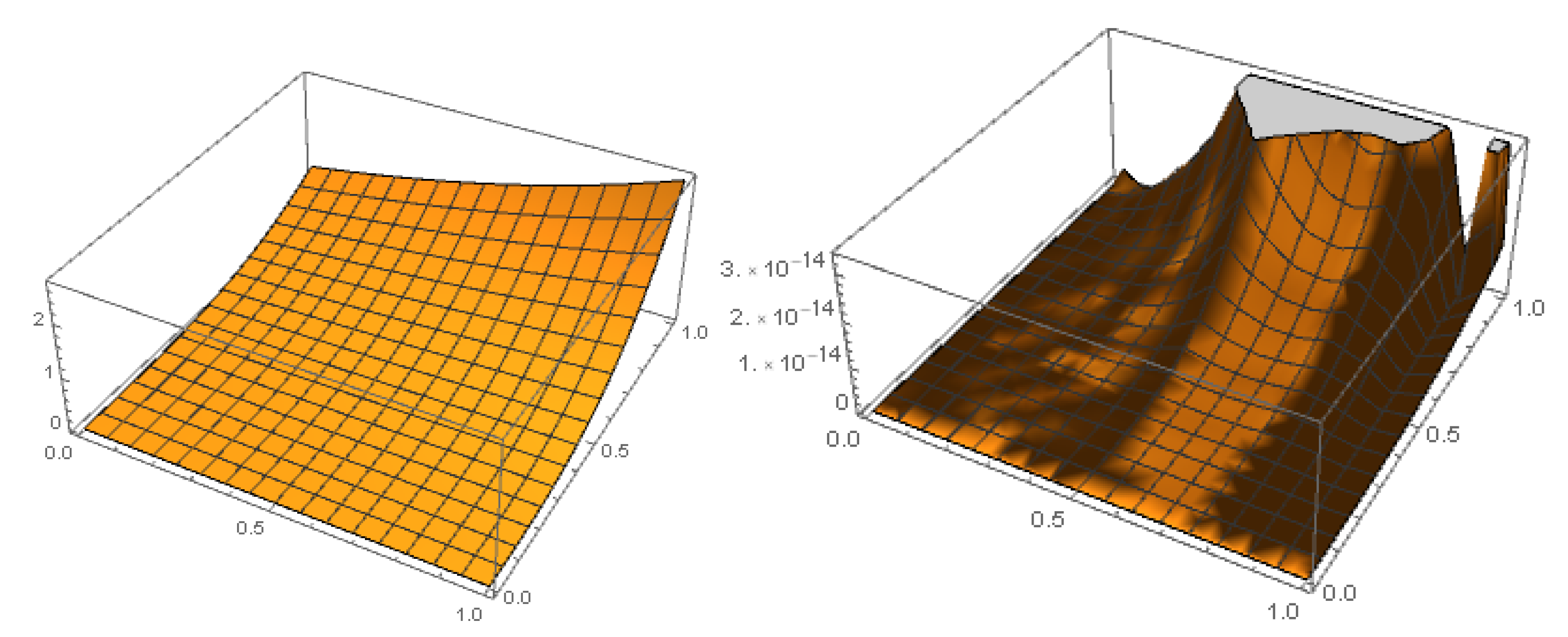
Figure 2.
The graph of the numerical solution (left) and the AEF (right) in Example 3 with .
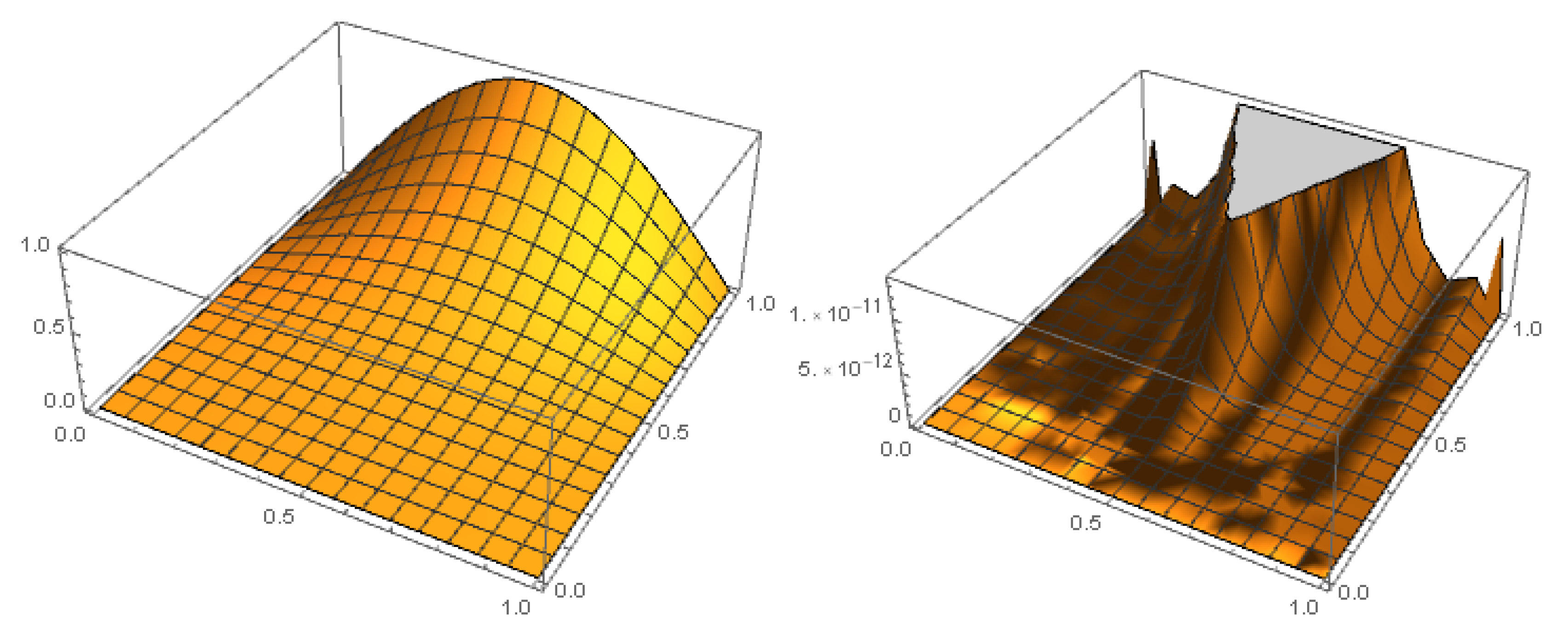
Figure 3.
The numerical solution of Example 4 with , and .
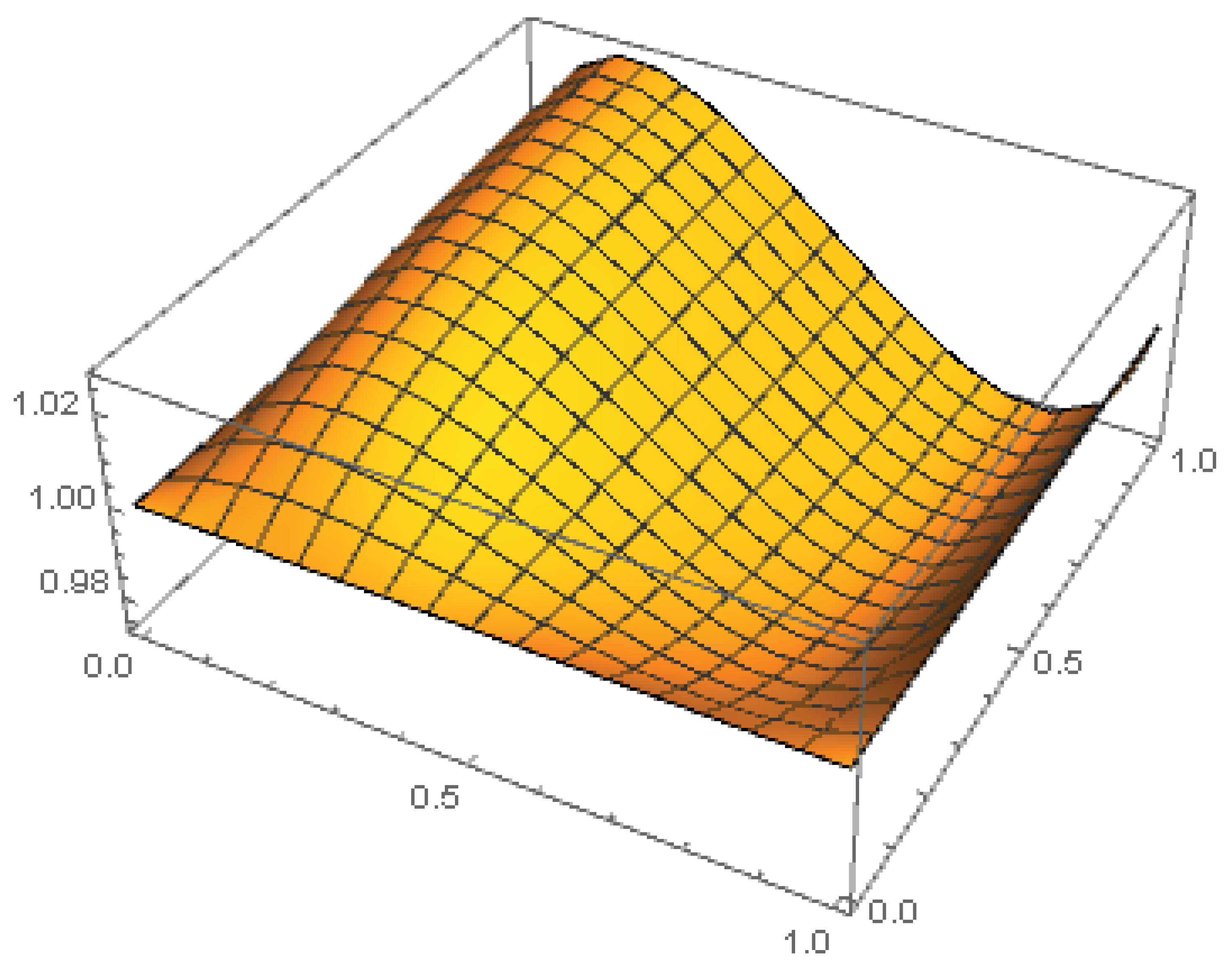

Table 1.
The relative errors for Example 2 with and various values of .
| 1 | ||||||
|---|---|---|---|---|---|---|
Table 2.
The relative errors for Example 2 with and various values of in comparison with the method in [36].
Table 2.
The relative errors for Example 2 with and various values of in comparison with the method in [36].
| Method in [36] | Present method with | |||||
|---|---|---|---|---|---|---|
Table 3.
The AEF of the numerical solution for Example 3 with , and various values of .
| 1 | |||||||
|---|---|---|---|---|---|---|---|
| 1 | |||||||
| 2 | |||||||
Table 4.
The REs of the approximated solution for Example 3 with , , and different values of in comparison with the method in [36].
Table 4.
The REs of the approximated solution for Example 3 with , , and different values of in comparison with the method in [36].
| Method in [36] | Present method | |||||
|---|---|---|---|---|---|---|
Table 5.
The REs of the numerical solution for Example 3 with , , and several values of in comparison with the result in [36].
Table 5.
The REs of the numerical solution for Example 3 with , , and several values of in comparison with the result in [36].
| Method in [36] | Present method | |||||
|---|---|---|---|---|---|---|
Table 6.
The maximal residual errors for Example 4 with , , and .
| MaxRE | CO | |
|---|---|---|
| 1 | − | |
| 2 | ||
| 3 | ||
| 4 | ||
| 5 |
Disclaimer/Publisher’s Note: The statements, opinions and data contained in all publications are solely those of the individual author(s) and contributor(s) and not of MDPI and/or the editor(s). MDPI and/or the editor(s) disclaim responsibility for any injury to people or property resulting from any ideas, methods, instructions or products referred to in the content. |
© 2025 by the authors. Licensee MDPI, Basel, Switzerland. This article is an open access article distributed under the terms and conditions of the Creative Commons Attribution (CC BY) license (http://creativecommons.org/licenses/by/4.0/).
Copyright: This open access article is published under a Creative Commons CC BY 4.0 license, which permit the free download, distribution, and reuse, provided that the author and preprint are cited in any reuse.


