Efficient Numerical Methods for Time-Fractional Diffusion Equations with Caputo-Type Erd\’{e}lyi-Kober Operator

1. Introduction

In recent decades, fractional integro-differential equations have emerged as critical mathematical tools in interdisciplinary scientific and engineering research [2,6,7,11]. Within this framework, fractional diffusion equations occupy a central position due to their capability to model anomalous transport phenomena. These equations exhibit remarkable versatility in capturing multi-regime diffusion dynamics and characteristic crossover behaviors observed in complex heterogeneous systems [10,12,14]. To address such diverse physical scenarios, multiple fractional operator definitions have been developed, including the Riemann-Liouville calculus, Grünwald-Letnikov integral, Caputo derivative, Hadamard calculus, Erdélyi-Kober calculus and so on. While numerical methods for equations involving the first four operator types have reached considerable maturity, the analysis of Erdélyi-Kober fractional operators remains an open research frontier. This gap in existing literature serves as the primary motivation for our work on developing systematic numerical approaches for this understudied operator class.

The Erdélyi-Kober fractional integral operator, originally introduced by Erdélyi and Hermann K. in 1940 [3] through integral boundary condition formulations, has gained significant traction in modeling multiscale physical systems [13,16,20]. Fundamental properties of these operators, particularly the relationship between Caputo-type Erdélyi-Kober derivatives and their classical counterparts, are systematically detailed in [6,9,21]. Recent advances in Erdélyi-Kober fractional integro-differential equations have yielded several key developments. [22,23] used the fixed point theorem to analyze the existence and uniqueness of solutions for Erdélyi-Kober fractional nonlinear integral equations. Płociniczak [17] established a dimension-reduction framework for fractional porous media equations via non-dimensionalization, transforming the original equation into tractable integro-differential forms, thus greatly reducing the complexity of the solution. Moreover, the Erdélyi-Kober operator’s equivalence to hyper-Bessel differential operators has enabled novel solution strategies for hyper-Bessel fractional equations [1,24,25].

The inherent non-locality of fractional operators renders analytical solutions computationally prohibitive, necessitating advanced numerical approximations for practical applications. While significant progress has been made in temporal fractional diffusion equations through finite difference [26], finite element [5], and spectral methods [8], numerical treatments for Erdélyi-Kober fractional integro-differential equations remain underdeveloped. Current limitations in this domain include: Płociniczak et al. [19] proposed rectangular, midpoint, and trapezoidal formulations for Erdélyi-Kober fractional integral operator, but provided no error bounds or theoretical justification. Odibat et al. [15] implemented predictor-correction method for Caputo-type Erdélyi-Kober fractional differential equations without convergence analysis. Existing semi-discrete schemes [18] achieve suboptimal first-order accuracy under initial weak regularity assumptions, and analyzed the stability and convergence of the scheme by using the Galerkin-Hermite method. Motivated by these gaps, this work develops novel high-order finite difference schemes for Caputo-type Erdélyi-Kober fractional diffusion equations, specifically targeting second-order temporal accuracy while maintaining rigorous stability guarantees through innovative kernel coefficient analysis.

In what follows, we focus on the following initial-boundary value problem of Caputo-type Erdélyi-Kober time fractional diffusion model in which $f,\phi$ are given suitably smooth functions, Caputo-type Erdélyi-Kober fractional derivative _CEK${\mathrm{D}}_{0,t;\sigma ,\eta }^{\alpha }p\left(t\right)$ is defined by [15]

$${}_{CEK}\mathrm{D}_{0,t;\sigma ,\eta }^{\alpha }p\left(t\right)={\displaystyle \frac{t^{-\sigma \eta }}{\Gamma (1-\alpha )}}{\int }_0^t{(t^{\sigma }-s^{\sigma })}^{-\alpha }{\delta }_{\sigma }\left[s^{\sigma (\alpha +\eta )}p\left(s\right)\right]\mathrm{d}{s}^{\sigma },\alpha \in (0,1),\sigma >0,\eta \in \mathbb{R},$$

(4)

where ${\delta }_{\sigma }={\displaystyle \frac{1}{\sigma s^{\sigma -1}}}{\displaystyle \frac{\mathrm{d}}{\mathrm{d}s}}.$

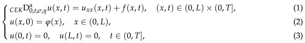To facilitate subsequent analysis, we apply Erdélyi-Kober fractional integral ${}_{CEK}\mathrm{D}_{0,t;\sigma ,\eta }^{\alpha }$ to both sides of (1), yielding an equivalent form

$$u(x,t){=}_{EK}{\mathrm{D}}_{0,t;\sigma ,\eta }^{-\alpha }{u}_{xx}(x,t)+F(x,t),(x,t)\in (0,L)\times (0,T],$$

(5)

where

$${}_{EK}\mathrm{D}_{0,t;\sigma ,\eta }^{-\alpha }{u}_{xx}(x,t)={\displaystyle \frac{t^{-\sigma (\alpha +\eta )}}{\Gamma \left(\alpha \right)}}{\int }_0^t{(t^{\sigma }-s^{\sigma })}^{\alpha -1}{s}^{\sigma \eta }{u}_{xx}(x,s)\mathrm{d}{s}^{\sigma },$$

$$F(x,t)={\displaystyle \frac{t^{-\sigma (\alpha +\eta )}}{\Gamma \left(\alpha \right)}}{\int }_0^t{(t^{\sigma }-s^{\sigma })}^{\alpha -1}{s}^{\sigma \eta }f(x,s)\mathrm{d}{s}^{\sigma }.$$

The remainder of this paper is organized as follows. Section 2 develops an L1-type discretization formula for the Erdélyi-Kober fractional integral operator, accompanied by a detailed analysis of truncation errors. Furthermore, we rigorously establish the positive definiteness of the discrete kernel coefficients. Building upon these theoretical foundations, we derive a finite difference scheme to solve (5). To enhance computational efficiency, Section 3 introduces a fast implementation algorithm for the difference scheme. The numerical example presented in Section 4 validate the theoretical predictions and demonstrate the effectiveness of our method. Finally, concluding remarks with perspectives are provided in the last section.

2. A Direct L1 Difference Scheme

This section focuses on constructing an L1-type difference scheme for Equation (5) coupled with its governing initial-boundary value conditions (2)-(3). We firstly introduce some spatial notations. Given a positive constant $M,$ denote $h=L/M.$ Let $x_i=ih(0\le i\le M),$${\Omega }_h=\left\{x_i\right|0\le i\le M\}.$ Then the grid function space is defined by

$${\mathcal{V}}_h=\left\{u\right|u=(u_0,u_1,\cdots ,u_M)\},{\stackrel{\circ }{\mathcal{V}}}_h=\left\{u\right|u\in {\mathcal{V}}_h;u_0=u_M=0\}.$$

For any $u\in {\mathcal{V}}_h,$ introduce the following notations,

$${\delta }_x{u}_{i-{\displaystyle \frac{1}{2}}}={\displaystyle \frac{1}{h}}(u_i-u_{i-1}),{\delta }_x^2{u}_i={\displaystyle \frac{1}{h^2}}(u_{i+1}-2u_i+u_{i-1}).$$

For any $u,v\in {\stackrel{\circ }{\mathcal{V}}}_h$, the inner products and norms are defined by

$$(u,v)=h\sum _{i=1}^{M-1}{u}_i{v}_i,\parallel u\parallel =\sqrt{(u,u)},$$

$$({\delta }_{x}u,{\delta }_{x}v)=h\sum _{i=1}^M{\delta }_x{u}_{i-{\displaystyle \frac{1}{2}}}{\delta }_x{v}_{i-{\displaystyle \frac{1}{2}}},\parallel {\delta }_{x}u\parallel =\sqrt{({\delta }_{x}u,{\delta }_{x}u)}.$$

2.1. The Derivation of the Difference Scheme

For any fixed $T,$ take a positive integer $N.$ And denote $\tau =T^{\sigma }/N,$$t_0=0,$$t_k={(t_{k-1}^{\sigma }+\tau )}^{{\displaystyle \frac{1}{\sigma }}},k=1,2,\cdots ,N.$

Denote $g(x,t)\triangleq t^{\sigma \eta }{u}_{xx}(x,t).$ Considering Equation (5) at the point $t=t_n,$ we have

$$\begin{array}{cc}\hfill u(x,t_n)=& {\displaystyle \frac{t_n^{-\sigma (\alpha +\eta )}}{\Gamma \left(\alpha \right)}}{\int }_0^{t_n}{(t_n^{\sigma }-s^{\sigma })}^{\alpha -1}g(x,s)\mathrm{d}{s}^{\sigma }+F(x,t_n)\hfill \\ \hfill =& {\displaystyle \frac{t_n^{-\sigma (\alpha +\eta )}}{\Gamma \left(\alpha \right)}}\sum _{k=0}^{n-1}{\int }_{t_k}^{t_{k+1}}{(t_n^{\sigma }-s^{\sigma })}^{\alpha -1}g(x,s)\mathrm{d}{s}^{\sigma }+F(x,t_n),x\in (0,L),1\le n\le N.\hfill \end{array}$$

(6)

Let ${\Pi }_{1,k}p\left(s\right)$ be linear interpolation polynomial of any function p defined on an interval $[t_k,t_{k+1}],k=0,1,\cdots ,N-1.$ We get

$${\Pi }_{1,k}p\left(s\right)={\displaystyle \frac{t_{k+1}^{\sigma }-s^{\sigma }}{\tau }}p\left(t_k\right)+{\displaystyle \frac{s^{\sigma }-t_k^{\sigma }}{\tau }}p\left(t_{k+1}\right),$$

(7)

with the truncation error

$${\theta }_p\left(s\right)={\Pi }_{1,k}p\left(s\right)-p\left(s\right)={\displaystyle \frac{1}{2}}(s^{\sigma }-t_{k+1}^{\sigma })(s^{\sigma }-t_k^{\sigma }){\delta }_{\sigma }^{2}p\left({\xi }_k\left(s\right)\right),{\xi }_k\left(s\right)\in (t_k,t_{k+1}),0\le k\le N.$$

(8)

We now develop an L1-type discretization formula for the temporal convolution integral in (6). Let we ignore the space variable x for a while. Using (7) we have

$$\begin{array}{cc}\hfill & {}_{EK}D_{0,t;\sigma ,\eta }^{-\alpha }{g\left(t\right)|}_{t=t_n}={\displaystyle \frac{t_n^{-\sigma (\alpha +\eta )}}{\Gamma \left(\alpha \right)}}\sum _{k=0}^{n-1}{\int }_{t_k}^{t_{k+1}}{(t_n^{\sigma }-s^{\sigma })}^{\alpha -1}g\left(s\right)\mathrm{d}{s}^{\sigma }\hfill \\ \hfill \approx & {\displaystyle \frac{t_n^{-\sigma (\alpha +\eta )}}{\Gamma \left(\alpha \right)}}\sum _{k=0}^{n-1}{\int }_{t_k}^{t_{k+1}}{(t_n^{\sigma }-s^{\sigma })}^{\alpha -1}\left[{\displaystyle \frac{t_{k+1}^{\sigma }-s^{\sigma }}{\tau }}g\left(t_k\right)+{\displaystyle \frac{s^{\sigma }-t_k^{\sigma }}{\tau }}g\left(t_{k+1}\right)\right]\mathrm{d}{s}^{\sigma }\hfill \\ \hfill =& {\displaystyle \frac{t_n^{-\sigma (\alpha +\eta )}}{\Gamma \left(\alpha \right)}}\sum _{k=0}^{n-1}\left[{\int }_{t_k}^{t_{k+1}}{(t_n^{\sigma }-s^{\sigma })}^{\alpha -1}(t_{k+1}^{\sigma }-s^{\sigma })\mathrm{d}{s}^{\sigma }{\displaystyle \frac{g\left(t_k\right)}{\tau }}+{\int }_{t_k}^{t_{k+1}}{(t_n^{\sigma }-s^{\sigma })}^{\alpha -1}(s^{\sigma }-t_k^{\sigma })\mathrm{d}{s}^{\sigma }{\displaystyle \frac{g\left(t_{k+1}\right)}{\tau }}\right]\hfill \\ \hfill =& {\displaystyle \frac{t_n^{-\sigma (\alpha +\eta )}}{\Gamma \left(\alpha \right)}}[{\displaystyle \frac{1}{\alpha (\alpha +1)}}{A}_{n,n-1}^{(\sigma ,\alpha )}{\displaystyle \frac{g\left(t_n\right)}{\tau }}+\sum _{k=1}^{n-1}{\displaystyle \frac{1}{\alpha (\alpha +1)}}(A_{n,k-1}^{(\sigma ,\alpha )}-A_{n,k}^{(\sigma ,\alpha )}){\displaystyle \frac{g\left(t_k\right)}{\tau }}\hfill \\ \hfill & +\left(-{\displaystyle \frac{A_{n,0}^{(\sigma ,\alpha )}}{\alpha (\alpha +1)}}+{\displaystyle \frac{\tau }{\alpha }}{t}_n^{\sigma \alpha }\right){\displaystyle \frac{g\left(t_0\right)}{\tau }}]\hfill \\ \hfill =& {\displaystyle \frac{t_n^{-\sigma (\alpha +\eta )}}{\Gamma \left(\alpha \right)}}\sum _{k=0}^n{C}_{n,k}^{(\sigma ,\alpha )}{\displaystyle \frac{g\left(t_k\right)}{\tau }}\triangleq {}_{EK}\mathbb{D}_{0,t;\sigma ,\eta }^{™\alpha }g\left(t_n\right),\hfill \end{array}$$

(9)

here

$$A_{n,k}^{(\sigma ,\alpha )}={(t_n^{\sigma }-t_k^{\sigma })}^{\alpha +1}-{(t_n^{\sigma }-t_{k+1}^{\sigma })}^{\alpha +1},0\le k\le n-1,$$

$$C_{n,k}^{(\sigma ,\alpha )}=\left\{\begin{array}{c}{\displaystyle \frac{\tau }{\alpha }}{t}_n^{\sigma \alpha }-{\displaystyle \frac{1}{\alpha (\alpha +1)}}\left[t_n^{\sigma (\alpha +1)}-{(t_n^{\sigma }-t_1^{\sigma })}^{\alpha +1}\right],k=0,\hfill \\ {\displaystyle \frac{1}{\alpha (\alpha +1)}}\left[{(t_n^{\sigma }-t_{k-1}^{\sigma })}^{\alpha +1}-2{(t_n^{\sigma }-t_k^{\sigma })}^{\alpha +1}+{(t_n^{\sigma }-t_{k+1}^{\sigma })}^{\alpha +1}\right],1\le k\le n-1,\hfill \\ {\displaystyle \frac{1}{\alpha (\alpha +1)}}{\tau }^{\alpha +1},k=n.\hfill \end{array}\right.$$

For the truncation error of the L1 formula ${}_{CEK}\mathbb{D}_{0,t;\sigma ,\eta }^{\alpha }g\left(t_n\right),$ we have the estimation below.

Theorem 1. 

Suppose $g\in C^2[t_0,t_n],$$\alpha \in (0,1).$ Denote

$$r_n={}_{EK}\mathbb{D}_{0,t;\sigma ,\eta }^{™\alpha }{g\left(t\right)|}_{t=t_n}-{}_{EK}\mathbb{D}_{0,t;\sigma ,\eta }^{™\alpha }g\left(t_n\right),n=1,2,\cdots ,N.$$

Then, we have

$$|r_n|\le {\displaystyle \frac{t_n^{-\sigma \eta }}{8\Gamma (1+\alpha )}}\underset{t_0<{\xi }_k\left(s\right)<t_n}{max}\left|{\delta }_{\sigma }^{2}g\left({\delta }_k\left(s\right)\right)\right|{\tau }^2.$$

Proof. 

With the help of (8), we get

$$\begin{array}{cc}\hfill |r_n|=& {\displaystyle \frac{t_n^{-\sigma (\alpha +\eta )}}{\Gamma \left(\alpha \right)}}\sum _{k=0}^{n-1}{\int }_{t_k}^{t_{k+1}}{(t_n^{\sigma }-s^{\sigma })}^{\alpha -1}|g\left(s\right)-{\Pi }_{1,k}g\left(s\right)|\mathrm{d}{s}^{\sigma }\hfill \\ \hfill \le & {\displaystyle \frac{t_n^{-\sigma (\alpha +\eta )}}{2\Gamma \left(\alpha \right)}}\sum _{k=0}^{n-1}{\int }_{t_k}^{t_{k+1}}{(t_n^{\sigma }-s^{\sigma })}^{\alpha -1}(t_{k+1}^{\sigma }-s^{\sigma })(s^{\sigma }-t_k^{\sigma })\left|{\delta }_{\sigma }^{2}g\left({\xi }_k\left(s\right)\right)\right|\mathrm{d}{s}^{\sigma }\hfill \\ \hfill \le & {\displaystyle \frac{t_n^{-\sigma (\alpha +\eta )}}{8\Gamma \left(\alpha \right)}}{\tau }^2\underset{t_0<{\xi }_k\left(s\right)<t_n}{max}\left|{\delta }_{\sigma }^{2}g\left({\xi }_k\left(s\right)\right)\right|\sum _{k=0}^{n-1}{\int }_{t_k}^{t_{k+1}}{(t_n^{\sigma }-s^{\sigma })}^{\alpha -1}\mathrm{d}{s}^{\sigma }\hfill \\ \hfill =& {\displaystyle \frac{t_n^{-\sigma \eta }}{8\Gamma (1+\alpha )}}\underset{t_0<{\xi }_k\left(s\right)<t_n}{max}\left|{\delta }_{\sigma }^{2}g\left({\xi }_k\left(s\right)\right)\right|{\tau }^2.\hfill \end{array}$$

Thus, we complete the proof. □

The coefficients $\left\{C_{n,k}^{(\sigma ,\alpha )}\right\}$ defined in (9) have the properties below.

Lemma 1. 

For $\left\{C_{n,k}^{(\sigma ,\alpha )}{|}_{k=0}^n\right\}$ defined in (9), it holds that

$$\begin{array}{cc}\hfill & 2C_{n,n}^{(\sigma ,\alpha )}>C_{n,n-1}^{(\sigma ,\alpha )}>\cdots >C_{n,2}^{(\sigma ,\alpha )}>C_{n,1}^{(\sigma ,\alpha )}>2C_{n,0}^{(\sigma ,\alpha )}>0;\hfill \end{array}$$

(10)

$$\begin{array}{cc}\hfill & C_{n,k}^{(\sigma ,\alpha )}-2C_{n,k-1}^{(\sigma ,\alpha )}+C_{n,k-2}^{(\sigma ,\alpha )}>0,3\le k\le n-1;\hfill \end{array}$$

(11)

$$\begin{array}{cc}\hfill & 2C_{n,0}^{(\sigma ,\alpha )}-2C_{n,1}^{(\sigma ,\alpha )}+C_{n,2}^{(\sigma ,\alpha )}>0,C_{n,n-2}^{(\sigma ,\alpha )}-2C_{n,n-1}^{(\sigma ,\alpha )}+2C_{n,n}^{(\sigma ,\alpha )}>0.\hfill \end{array}$$

(12)

Proof. 

(1) Proof of (10). It is easy to know that

$$C_{n,0}^{(\sigma ,\alpha )}={\displaystyle \frac{\tau }{\alpha }}\left[t_n^{\sigma \alpha }-{(t_n^{\sigma }-{\xi }_1)}^{\alpha }\right]>{\displaystyle \frac{\tau }{\alpha }}\left[t_n^{\sigma \alpha }-t_n^{\sigma \alpha }\right]=0,{\xi }_1\in (0,t_1^{\sigma }).$$

For $2\le k\le n-1,$ we have

$$\begin{array}{cc}\hfill & C_{n,k}^{(\sigma ,\alpha )}-C_{n,k-1}^{(\sigma ,\alpha )}\hfill \\ \hfill =& {\displaystyle \frac{1}{\alpha (\alpha +1)}}\left[-{(t_n^{\sigma }-t_{k-2}^{\sigma })}^{\alpha +1}+3{(t_n^{\sigma }-t_{k-1}^{\sigma })}^{\alpha +1}-3{(t_n^{\sigma }-t_k^{\sigma })}^{\alpha +1}+{(t_n^{\sigma }-t_{k+1}^{\sigma })}^{\alpha +1}\right]\hfill \\ \hfill =& (1-\alpha ){\int }_0^{\tau }\mathrm{d}{z}_1{\int }_0^{\tau }\mathrm{d}{z}_2{\int }_0^{\tau }{(t_n^{\sigma }-t_{k+1}^{\sigma }+z_1+z_2+z_3)}^{\alpha -2}\mathrm{d}{z}_3>0.\hfill \\ \hfill & 2C_{n,n}^{(\sigma ,\alpha )}-C_{n,n-1}^{(\sigma ,\alpha )}\hfill \\ \hfill =& {\displaystyle \frac{2}{\alpha (\alpha +1)}}{\tau }^{\alpha +1}-{\displaystyle \frac{1}{\alpha (\alpha +1)}}\left[{(t_n^{\sigma }-t_{n-2}^{\alpha })}^{\alpha +1}-2{\tau }^{\alpha +1}\right]\hfill \\ \hfill =& {\displaystyle \frac{{\tau }^{\alpha +1}}{\alpha (\alpha +1)}}[4-2^{\alpha +1}]>0.\hfill \\ \hfill & C_{n,1}^{(\sigma ,\alpha )}-2C_{n,0}^{(\sigma ,\alpha )}\hfill \\ \hfill =& {\displaystyle \frac{1}{\alpha (\alpha +1)}}\left[3t_n^{\sigma (\alpha +1)}-4{(t_n^{\sigma }-t_1^{\sigma })}^{\alpha +1}+{(t_n^{\sigma }-t_2^{\sigma })}^{\alpha +1}\right]-{\displaystyle \frac{2\tau }{\alpha }}{t}_n^{\sigma \alpha }\hfill \\ \hfill =& {\displaystyle \frac{{\tau }^{\alpha +1}}{\alpha }}P(n,\alpha ),\hfill \end{array}$$

where $P(n,\alpha )={\displaystyle \frac{1}{\alpha +1}}\left[3n^{\alpha +1}-4{(n-1)}^{\alpha +1}+{(n-2)}^{\alpha +1}\right]-2n^{\alpha }.$ To prove $C_{n,1}^{(\sigma ,\alpha )}-2C_{n,0}^{(\sigma ,\alpha )}>0,$ we just need to prove $P(n,\alpha )>0.$ By Taylor’s formula, we have

$$\begin{array}{cc}\hfill P(n,\alpha )=& {\displaystyle \frac{1}{\alpha +1}}[3n^{\alpha +1}-4n^{\alpha +1}+4(\alpha +1)n^{\alpha }-2\alpha (\alpha +1)n^{\alpha -1}-{\displaystyle \frac{2}{3}}\alpha (\alpha +1)(1-\alpha ){(n-1+{\xi }_1)}^{\alpha -2}\hfill \\ \hfill & +n^{\alpha +1}-2(\alpha +1)n^{\alpha }+2\alpha (\alpha +1)n^{\alpha -1}+{\displaystyle \frac{4}{3}}\alpha (\alpha +1)(1-\alpha ){(n-2+{\xi }_2)}^{\alpha -2}]-2n^{\alpha }\hfill \\ \hfill =& {\displaystyle \frac{2}{3}}\alpha (1-\alpha )\left[2{(n-2+{\xi }_2)}^{\alpha -2}-{(n-1+{\xi }_1)}^{\alpha -2}\right],\hfill \end{array}$$

in which ${\xi }_1\in (0,1),{\xi }_2\in (0,2).$

It is easy to know that

$$P(n,\alpha )>{\displaystyle \frac{2}{3}}\alpha (1-\alpha )[2n^{\alpha -2}-{(n-1)}^{\alpha -2}]>0\mathrm{for}n\ge 4.$$

In addition, when $n=2,3,$$P(n,\alpha )>0$ can be proved by a simple calculation.

(2) Proof of (11).

$$\begin{array}{cc}\hfill & C_{n,k}^{(\sigma ,\alpha )}-2C_{n,k-1}^{(\sigma ,\alpha )}+C_{n,k-2}^{(\sigma ,\alpha )}\hfill \\ \hfill =& {\displaystyle \frac{1}{\alpha (\alpha +1)}}\left[{(t_n^{\sigma }-t_{k-3}^{\sigma })}^{\alpha +1}-4{(t_n^{\sigma }-t_{k-2}^{\sigma })}^{\alpha +1}+6{(t_n^{\sigma }-t_{k-1}^{\sigma })}^{\alpha +1}-4{(t_n^{\sigma }-t_k^{\sigma })}^{\alpha +1}+{(t_n^{\sigma }-t_{k+1}^{\sigma })}^{\alpha +1}\right]\hfill \\ \hfill =& (1-\alpha )(2-\alpha ){\int }_0^{\tau }\mathrm{d}{z}_1{\int }_0^{\tau }\mathrm{d}{z}_2{\int }_0^{\tau }\mathrm{d}{z}_3{\int }_0^{\tau }{(t_n^{\sigma }-t_{k+1}^{\sigma }+z_1+z_2+z_3+z_4)}^{\alpha -3}\mathrm{d}{z}_4>0.\hfill \end{array}$$

(3) Proof of (12).

$$\begin{array}{cc}\hfill & 2C_{n,0}^{(\sigma ,\alpha )}-2C_{n,1}^{(\sigma ,\alpha )}+C_{n,2}^{(\sigma ,\alpha )}\hfill \\ \hfill =& {\displaystyle \frac{2\tau }{\alpha }}{t}_n^{\sigma \alpha }+{\displaystyle \frac{1}{\alpha (\alpha +1)}}\left[-4t_n^{\sigma (\alpha +1)}+7{(t_n^{\sigma }-t_1^{\sigma })}^{\alpha +1}-4{(t_n^{\sigma }-t_2^{\sigma })}^{\alpha +1}+{(t_n^{\sigma }-t_3^{\sigma })}^{\alpha +1}\right]\hfill \\ \hfill =& {\displaystyle \frac{{\tau }^{\alpha +1}}{\alpha }}\left\{2n^{\alpha }+{\displaystyle \frac{1}{\alpha +1}}\left[-4n^{\alpha +1}+7{(n-1)}^{\alpha +1}-4{(n-2)}^{\alpha +1}+{(n-3)}^{\alpha +1}\right]\right\}.\hfill \end{array}$$

Similar to the treatment of $P(n,\alpha ),$ one can also prove that $2C_{n,0}^{(\sigma ,\alpha )}-2C_{n,1}^{(\sigma ,\alpha )}+C_{n,2}^{(\sigma ,\alpha )}>0.$

$$\begin{array}{cc}\hfill & C_{n,n-2}^{(\sigma ,\alpha )}-2C_{n,n-1}^{(\sigma ,\alpha )}+2C_{n,n}^{(\sigma ,\alpha )}\hfill \\ \hfill =& {\displaystyle \frac{1}{\alpha (\alpha +1)}}\left[{(t_n^{\sigma }-t_{n-3}^{\sigma })}^{\alpha +1}-4{(t_n^{\sigma }-t_{n-2}^{\sigma })}^{\alpha +1}+7{\tau }^{\alpha +1}\right]\hfill \\ \hfill =& {\displaystyle \frac{{\tau }^{\alpha +1}}{\alpha (\alpha +1)}}\left(3^{\alpha +1}-4·2^{\alpha +3}+7\right)>0.\hfill \end{array}$$

Therefore, the proof is complete. □

Now, we devote to presenting a second-order difference scheme for solving the problem (1)-(3). Suppose $u(x,t)\in C^{(4,2)}([0,L]\times [0,T]).$ Denote

$$U_i^n=u(x_i,t_n),F_i^n=F(x_i,t_n),0\le n\le N;{\phi }_i=\phi \left(x_i\right),0\le i\le M.$$

Considering Equation (5) at the point $(x_i,t_n),$ we get

$$u(x_i,t_n)={\displaystyle \frac{t_n^{-\sigma (\alpha +\eta )}}{\Gamma \left(\alpha \right)}}{\int }_0^{t_n}{(t_n^{\sigma }-s^{\sigma })}^{\alpha -1}{s}^{\sigma \eta }{u}_{xx}(x_i,s)\mathrm{d}{s}^{\sigma }+F(x_i,t_n),1\le i\le M-1,1\le n\le N.$$

Applying (9) to approximating the temporal fractional derivative and central difference quotient to the spatial derivative, we can obtain

$$U_i^n={\displaystyle \frac{t_n^{-\sigma (\alpha +\eta )}}{\Gamma \left(\alpha \right)}}\sum _{k=0}^n{C}_{n,k}^{(\sigma ,\alpha )}{\displaystyle \frac{t_k^{\sigma \eta }}{\tau }}{\delta }_x^2{U}_i^k+F_i^n+R_i^n,1\le i\le M-1,1\le n\le N,$$

(13)

where

$$R_i^n=r_i^n+{\displaystyle \frac{t_n^{-\sigma (\alpha +\eta )}}{\Gamma \left(\alpha \right)}}\sum _{k=0}^n{C}_{n,k}^{(\sigma ,\alpha )}{\displaystyle \frac{t_k^{\sigma \eta }}{\tau }}\left[u_{xx}(x_i,t_k)-{\delta }_x^2{U}_i^k\right]$$

Noticing Theorem 1, there exists a positive constant $c_1$ such that

$$\begin{array}{cc}\hfill |R_i^k|\le & |r_i^n|+{\displaystyle \frac{c_1{t}_n^{-\sigma \alpha }}{\Gamma \left(\alpha \right)\tau }}{h}^2\sum _{k=0}^n{C}_{n,k}^{(\sigma ,\alpha )}\hfill \\ \hfill \le & {\displaystyle \frac{t_n^{-\sigma \eta }}{8\Gamma (1+\alpha )}}\underset{t_0<{\xi }_k\left(s\right)<t_n}{max}\left|{\delta }_{\sigma }^{2}g\left({\delta }_k\left(s\right)\right)\right|{\tau }^2+{\displaystyle \frac{c_1{t}_n^{-\sigma \alpha }}{\Gamma \left(\alpha \right)\tau }}{h}^2·{\displaystyle \frac{\tau }{\alpha }}{t}_n^{\sigma \alpha }\hfill \\ \hfill =& {\displaystyle \frac{t_n^{-\sigma \eta }}{8\Gamma (1+\alpha )}}\underset{t_0<{\xi }_k\left(s\right)<t_n}{max}\left|{\delta }_{\sigma }^{2}g\left({\delta }_k\left(s\right)\right)\right|{\tau }^2+{\displaystyle \frac{c_1{h}^2}{\Gamma (\alpha +1)}}.\hfill \end{array}$$

(14)

Noticing the initial-boundary value conditions (2) and (3), we have Omitting the small terms in (13) and replacing the grid function $U_i^n$ by its numerical approximation $u_i^n,$ we construct a direct second-order difference scheme for solving the problem (1)-(3) as follows:

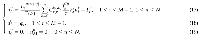3. A Fast Difference Scheme

The inherent non-locality of fractional operators poses significant implementation challenges in practical computation. To address this fundamental limitation, we implement the fast algorithm developed by Jiang et al. [4] within our methodological framework.

3.1. Fast Approximation of the Erdélyi-Kober Integral

The following lemma is fundamental and needed.

Lemma 2. 

[4] For the given $\gamma \in (0,1)$ and tolerance error $ϵ,$ cut-off time restriction $\delta$ and final time $T,$ there are one positive integer $N_{exp}^{\left(\gamma \right)},$ positive points $\left\{s_l^{\left(\gamma \right)}\right|l=1,2,\cdots ,N_{exp}^{\left(\gamma \right)}\},$ and corresponding positive weights $\left\{w_l^{\left(\gamma \right)}\right|l=1,2,\cdots ,N_{exp}^{\left(\gamma \right)}\}$ such that

$$|t^{-\gamma }-\sum _{l=1}^{N_{exp}^{\left(\gamma \right)}}{w}_l^{\left(\gamma \right)}{e}^{-s_l^{\left(\gamma \right)}t}|\le ϵ,\forall t\in [\delta ,T],$$

where

$$N_{exp}^{\left(\gamma \right)}=O\left((log{\displaystyle \frac{1}{ϵ}})(loglog{\displaystyle \frac{1}{ϵ}}+log{\displaystyle \frac{T}{\delta }})+(log{\displaystyle \frac{1}{\delta }})(loglog{\displaystyle \frac{1}{ϵ}}+log{\displaystyle \frac{1}{\delta }})\right).$$

Now, we will derive a fast algorithm for computing the Erdélyi-Kober integral ${}_{CEK}D_{0,t;\sigma ,\eta }^{\alpha }{g\left(t\right)|}_{t=t_n}.$ Let $\delta =\tau /2.$

$$\begin{array}{cc}\hfill & {}_{EK}D_{0,t;\sigma ,\eta }^{-\alpha }{g\left(t\right)|}_{t=t_n}\hfill \\ \hfill =& {\displaystyle \frac{t_n^{-\sigma (\alpha +\eta )}}{\Gamma \left(\alpha \right)}}\sum _{k=0}^{n-1}{\int }_{t_k}^{t_{k+1}}{(t_n^{\sigma }-s^{\sigma })}^{\alpha -1}g\left(s\right)\mathrm{d}{s}^{\sigma }\hfill \\ \hfill =& {\displaystyle \frac{t_n^{-\sigma (\alpha +\eta )}}{\Gamma \left(\alpha \right)}}\left[\sum _{k=0}^{n-2}{\int }_{t_k}^{t_{k+1}}{(t_n^{\sigma }-s^{\sigma })}^{\alpha -1}g\left(s\right)\mathrm{d}{s}^{\sigma }+{\int }_{t_{n-1}}^{t_n}{(t_n^{\sigma }-s^{\sigma })}^{\alpha -1}g\left(s\right)\mathrm{d}{s}^{\sigma }\right]\hfill \\ \hfill \approx & {\displaystyle \frac{t_n^{-\sigma (\alpha +\eta )}}{\Gamma \left(\alpha \right)}}\left[\sum _{l=1}^{N_{exp}^{(1-\alpha )}}{w}_l^{(1-\alpha )}\sum _{k=0}^{n-2}{\int }_{t_k}^{t_{k+1}}{e}^{-s_l^{(1-\alpha )}(t_n^{\sigma }-s^{\sigma })}{\Pi }_{1,k}g\left(s\right)\mathrm{d}{s}^{\sigma }+{\int }_{t_{n-1}}^{t_n}{(t_n^{\sigma }-s^{\sigma })}^{\alpha -1}{\Pi }_{1,n-1}g\left(s\right)\mathrm{d}{s}^{\sigma }\right]\hfill \\ \hfill =& {\displaystyle \frac{t_n^{-\sigma (\alpha +\eta )}}{\Gamma \left(\alpha \right)}}\left[\sum _{l=1}^{N_{exp}^{(1-\alpha )}}{w}_l^{(1-\alpha )}{F}_l^n+{\displaystyle \frac{{\tau }^{\alpha }}{\alpha +1}}g\left(t_{n-1}\right)+{\displaystyle \frac{{\tau }^{\alpha }}{\alpha (\alpha +1)}}g\left(t_n\right)\right],\hfill \end{array}$$

(20)

where

$$\begin{array}{cc}\hfill & F_l^1=0;\hfill \\ \hfill & F_l^n=\sum _{k=0}^{n-2}{\int }_{t_k}^{t_{k+1}}{e}^{-s_l^{(1-\alpha )}(t_n^{\sigma }-s^{\sigma })}{\Pi }_{1,k}g\left(s\right)\mathrm{d}{s}^{\sigma }.\hfill \end{array}$$

The integral $F_l^n$ can be evaluated by using a recursive algorithm, i.e.

$$\begin{array}{cc}\hfill F_l^n=& e^{-s_l^{(1-\alpha )}\tau }\sum _{k=0}^{n-3}{\int }_{t_k}^{t_{k+1}}{e}^{-s_l^{(1-\alpha )}(t_{n-1}^{\sigma }-s^{\sigma })}{\Pi }_{1,k}g\left(s\right)\mathrm{d}{s}^{\sigma }+{\int }_{t_{n-2}}^{t_{n-1}}{e}^{-s_l^{(1-\alpha )}(t_n^{\sigma }-s^{\sigma })}{\Pi }_{1,n-2}g\left(s\right)\mathrm{d}{s}^{\sigma }\hfill \\ \hfill =& e^{-s_l^{(1-\alpha )}\tau }{F}_l^{n-1}+A_l{\displaystyle \frac{g\left(t_{n-2}\right)}{\tau }}+B_l{\displaystyle \frac{g\left(t_{n-1}\right)}{\tau }},n=2,3,\cdots ,\hfill \end{array}$$

where for $1\le l\le N_{exp}^{(1-\alpha )},$

$$\begin{array}{cc}\hfill & A_l={\displaystyle \frac{1}{s_l^{(1-\alpha )}}}\left\{-\tau e^{-2s_l^{(1-\alpha )}\tau }+{\displaystyle \frac{1}{s_l^{(1-\alpha )}}}\left[e^{-s_l^{(1-\alpha )}\tau }-e^{-2s_l^{(1-\alpha )}\tau }\right]\right\},\hfill \\ \hfill & B_l={\displaystyle \frac{1}{s_l^{(1-\alpha )}}}\left\{\tau e^{-s_l^{(1-\alpha )}\tau }-{\displaystyle \frac{1}{s_l^{(1-\alpha )}}}\left[e^{-s_l^{(1-\alpha )}\tau }-e^{-2s_l^{(1-\alpha )}\tau }\right]\right\}.\hfill \end{array}$$

Besides, one can show that

$$\begin{array}{cc}\hfill & {}_{EK}D_{0,t;\sigma ,\eta }^{-\alpha }{g\left(t\right)|}_{t=t_n}\hfill \\ \hfill \approx & {\displaystyle \frac{t_n^{-\sigma (\alpha +\eta )}}{\Gamma \left(\alpha \right)}}[\sum _{l=1}^{N_{exp}^{(1-\alpha )}}{w}_l^{(1-\alpha )}\sum _{k=0}^{n-2}{\int }_{t_k}^{t_{k+1}}{e}^{-s_l^{(1-\alpha )}(t_n^{\sigma }-s^{\sigma })}\left({\displaystyle \frac{t_{k+1}^{\sigma }-s^{\sigma }}{\tau }}g\left(t_k\right)+{\displaystyle \frac{s^{\sigma }-t_k^{\sigma }}{\tau }}g\left(t_{k+1}\right)\right)\mathrm{d}{s}^{\sigma }\hfill \\ \hfill & +{\int }_{t_{n-1}}^{t_n}{(t_n^{\sigma }-s^{\sigma })}^{\alpha -1}\left({\displaystyle \frac{t_n^{\sigma }-s^{\sigma }}{\tau }}g\left(t_{n-1}\right)+{\displaystyle \frac{s^{\sigma }-t_{n-1}^{\sigma }}{\tau }}g\left(t_n\right)\right)\mathrm{d}{s}^{\sigma }]\hfill \\ \hfill =& {\displaystyle \frac{t_n^{-\sigma (\alpha +\eta )}}{\Gamma \left(\alpha \right)}}[{\int }_{t_{n-1}}^{t_n}{(t_n^{\sigma }-s^{\sigma })}^{\alpha -1}(s^{\sigma }-t_{n-1}^{\sigma })\mathrm{d}{s}^{\sigma }·{\displaystyle \frac{g\left(t_n\right)}{\tau }}\hfill \\ \hfill & +\left(\sum _{l=1}^{N_{exp}^{(1-\alpha )}}{w}_l^{(1-\alpha )}{\int }_{t_{n-2}}^{t_{n-1}}{e}^{-s_l^{(1-\alpha )}(t_n^{\sigma }-s^{\sigma })}(s^{\sigma }-t_{n-2}^{\sigma })\mathrm{d}{s}^{\sigma }+{\int }_{t_{n-1}}^{t_n}{(t_n^{\sigma }-s^{\sigma })}^{\alpha }\mathrm{d}{s}^{\sigma }\right)·{\displaystyle \frac{g\left(t_{n-1}\right)}{\tau }}\hfill \\ \hfill & +\sum _{l=1}^{N_{exp}^{(1-\alpha )}}{w}_l^{(1-\alpha )}\sum _{k=1}^{n-2}\left({\int }_{t_k}^{t_{k+1}}{e}^{-s_l^{(1-\alpha )}(t_n^{\sigma }-s^{\sigma })}(t_{k+1}^{\sigma }-s^{\sigma })\mathrm{d}{s}^{\sigma }+{\int }_{t_{k-1}}^{t_k}{e}^{-s_l^{(1-\alpha )}(t_n^{\sigma }-s^{\sigma })}(s^{\sigma }-t_{k-1}^{\sigma })\mathrm{d}{s}^{\sigma }\right)·{\displaystyle \frac{g\left(t_k\right)}{\tau }}\hfill \\ \hfill & +\sum _{l=1}^{N_{exp}^{(1-\alpha )}}{w}_l^{(1-\alpha )}{\int }_0^{t_1}{e}^{-s_l^{(1-\alpha )}(t_n^{\sigma }-s^{\sigma })}(t_1^{\sigma }-s^{\sigma })\mathrm{d}{s}^{\sigma }·{\displaystyle \frac{g\left(t_0\right)}{\tau }}]\hfill \\ \hfill =& {\displaystyle \frac{t_n^{-\sigma (\alpha +\eta )}}{\Gamma \left(\alpha \right)}}\sum _{k=0}^n{\widehat{C}}_{n,k}^{(\sigma ,\alpha )}{\displaystyle \frac{g\left(t_k\right)}{\tau }}\triangleq {}_{FEK}\mathbb{D}_{0,t;\sigma ,\eta }^{™\alpha }g\left(t_n\right),\hfill \end{array}$$

in which

$${\widehat{C}}_{n,k}^{(\sigma ,\alpha )}=\left\{\begin{array}{c}\sum _{l=1}^{N_{exp}^{(1-\alpha )}}{w}_l^{(1-\alpha )}{\int }_0^{t_1}{e}^{-s_l^{(1-\alpha )}(t_n^{\sigma }-s^{\sigma })}(t_1^{\sigma }-s^{\sigma })\mathrm{d}{s}^{\sigma },k=0,\hfill \\ \sum _{l=1}^{N_{exp}^{(1-\alpha )}}{w}_l^{(1-\alpha )}({\int }_{t_k}^{t_{k+1}}{e}^{-s_l^{(1-\alpha )}(t_n^{\sigma }-s^{\sigma })}(t_{k+1}^{\sigma }-s^{\sigma })\mathrm{d}{s}^{\sigma }\hfill \\ +{\int }_{t_{k-1}}^{t_k}{e}^{-s_l^{(1-\alpha )}(t_n^{\sigma }-s^{\sigma })}(s^{\sigma }-t_{k-1}^{\sigma })\mathrm{d}{s}^{\sigma }),1\le k\le n-2,\hfill \\ \sum _{l=1}^{N_{exp}^{(1-\alpha )}}{w}_l^{(1-\alpha )}{\int }_{t_{n-2}}^{t_{n-1}}{e}^{-s_l^{(1-\alpha )}(t_n^{\sigma }-s^{\sigma })}(s^{\sigma }-t_{n-2}^{\sigma })\mathrm{d}{s}^{\sigma }+{\displaystyle \frac{1}{\alpha +1}}{\tau }^{\alpha +1},k=n-1,\hfill \\ {\displaystyle \frac{1}{\alpha (\alpha +1)}}{\tau }^{\alpha +1},k=n.\hfill \end{array}\right.$$

By the definition of $C_{n,k}^{(\sigma ,\alpha )}$ and ${\widehat{C}}_{n,k}^{(\sigma ,\alpha )},$ it is easy to know that

$$C_{n,n}^{(\sigma ,\alpha )}-{\widehat{C}}_{n,n}^{(\sigma ,\alpha )}=0;|C_{n,k}^{(\sigma ,\alpha )}-{\widehat{C}}_{n,k}^{(\sigma ,\alpha )}|\le ϵ,0\le k\le n-1.$$

Lemma 3. 

The coefficient $\left\{{\widehat{C}}_{n,k}^{(\sigma ,\alpha )}{|}_{k=0}^n\right\}$ satisfies

$$\begin{array}{cc}\hfill & 2{\widehat{C}}_{n,n}^{(\sigma ,\alpha )}>{\widehat{C}}_{n,n-1}^{(\sigma ,\alpha )}>\cdots >{\widehat{C}}_{n,2}^{(\sigma ,\alpha )}>{\widehat{C}}_{n,1}^{(\sigma ,\alpha )}>2{\widehat{C}}_{n,0}^{(\sigma ,\alpha )}>0;\hfill \end{array}$$

(21)

$$\begin{array}{cc}\hfill & {\widehat{C}}_{n,k}^{(\sigma ,\alpha )}-2{\widehat{C}}_{n,k-1}^{(\sigma ,\alpha )}+{\widehat{C}}_{n,k-2}^{(\sigma ,\alpha )}>0,3\le k\le n-1;\hfill \end{array}$$

(22)

$$\begin{array}{cc}\hfill & 2{\widehat{C}}_{n,0}^{(\sigma ,\alpha )}-2{\widehat{C}}_{n,1}^{(\sigma ,\alpha )}+{\widehat{C}}_{n,2}^{(\sigma ,\alpha )}>0,{\widehat{C}}_{n,n-2}^{(\sigma ,\alpha )}-2{\widehat{C}}_{n,n-1}^{(\sigma ,\alpha )}+2{\widehat{C}}_{n,n}^{(\sigma ,\alpha )}>0.\hfill \end{array}$$

(23)

Proof. 

It is clear that all ${\widehat{C}}_{n,k}^{(\sigma ,\alpha )}$ are positive. For $1\le k\le n-2,$ the mean value theorem yields

$$\begin{array}{cc}\hfill & {\widehat{C}}_{n,k}^{(\sigma ,\alpha )}\hfill \\ \hfill =& \sum _{l=1}^{N_{exp}^{(1-\alpha )}}{w}_l^{(1-\alpha )}\left({\displaystyle \frac{1}{s_l^{(1-\alpha )}}}{\int }_{t_k^{\sigma }}^{t_{k+1}^{\sigma }}(t_{k+1}^{\sigma }-s)\mathrm{d}{e}^{-s_l^{(1-\alpha )}(t_n^{\sigma }-s)}+{\displaystyle \frac{1}{s_l^{(1-\alpha )}}}{\int }_{t_{k-1}^{\sigma }}^{t_k^{\sigma }}(s-t_{k-1}^{\sigma })\mathrm{d}{e}^{-s_l^{(1-\alpha )}(t_n^{\sigma }-s)}\right)\hfill \\ \hfill =& \sum _{l=1}^{N_{exp}^{(1-\alpha )}}{\displaystyle \frac{w_l^{(1-\alpha )}}{s_l^{(1-\alpha )}}}\left({\int }_{t_k^{\sigma }}^{t_{k+1}^{\sigma }}{e}^{-s_l^{(1-\alpha )}(t_n^{\sigma }-s)}\mathrm{d}s-{\int }_{t_{k-1}^{\sigma }}^{t_k^{\sigma }}{e}^{-s_l^{(1-\alpha )}(t_n^{\sigma }-s)}\mathrm{d}s\right)\hfill \\ \hfill =& \sum _{l=1}^{N_{exp}^{(1-\alpha )}}{\displaystyle \frac{w_l^{(1-\alpha )}}{s_l^{(1-\alpha )}}}{\int }_{t_k^{\sigma }}^{t_{k+1}^{\sigma }}{e}^{-s_l^{(1-\alpha )}(t_n^{\sigma }-s)}(1-e^{-s_l^{(1-\alpha )}\tau })\mathrm{d}s\hfill \\ \hfill =& \sum _{l=1}^{N_{exp}^{(1-\alpha )}}{\displaystyle \frac{w_l^{(1-\alpha )}}{s_l^{(1-\alpha )}}}(1-e^{-s_l^{(1-\alpha )}\tau })\tau e^{-s_l^{(1-\alpha )}(t_n^{\sigma }-{\xi }_k)},{\xi }_k\in (t_k^{\sigma },t_{k+1}^{\sigma }),\hfill \end{array}$$

which means that ${\widehat{C}}_{n,k}^{(\sigma ,\alpha )}$ increase monotonically with respect to k and is convex.

$$\begin{array}{cc}\hfill & {\widehat{C}}_{n,n-1}^{(\sigma ,\alpha )}-{\widehat{C}}_{n,n-2}^{(\sigma ,\alpha )}\hfill \\ \hfill =& \sum _{l=1}^{N_{exp}^{(1-\alpha )}}{w}_l^{(1-\alpha )}\left({\int }_{t_{n-2}^{\sigma }}^{t_{n-1}^{\sigma }}{e}^{-s_l^{(1-\alpha )}(t_n^{\sigma }-s)}(s-t_{n-2}^{\sigma })\mathrm{d}s-{\int }_{t_{n-3}^{\sigma }}^{t_{n-2}^{\sigma }}{e}^{-s_l^{(1-\alpha )}(t_n^{\sigma }-s)}(s-t_{n-3}^{\sigma })\mathrm{d}s\right)\hfill \\ \hfill & +{\displaystyle \frac{1}{\alpha +1}}{\tau }^{\alpha +1}-\sum _{l=1}^{N_{exp}^{(1-\alpha )}}{w}_l^{(1-\alpha )}{\int }_{t_{n-2}^{\sigma }}^{t_{n-1}^{\sigma }}{e}^{-s_l^{(1-\alpha )}(t_n^{\sigma }-s)}(t_{n-1}^{\sigma }-s)\mathrm{d}s\hfill \\ \hfill \ge & \sum _{l=1}^{N_{exp}^{(1-\alpha )}}{w}_l^{(1-\alpha )}{\int }_{t_{n-2}^{\sigma }}^{t_{n-1}^{\sigma }}{e}^{-s_l^{(1-\alpha )}(t_n^{\sigma }-s)}(s-t_{n-2}^{\sigma })(1-e^{-s_l^{(1-\alpha )}\tau })\mathrm{d}s\hfill \\ \hfill & +{\displaystyle \frac{1}{\alpha +1}}{\tau }^{\alpha +1}-{\int }_{t_{n-2}^{\sigma }}^{t_{n-1}^{\sigma }}\left[ϵ+{(t_n^{\sigma }-s)}^{\alpha -1}\right](t_{n-1}^{\sigma }-s)\mathrm{d}s\hfill \\ \hfill \ge & {\displaystyle \frac{{\tau }^{\alpha +1}}{\alpha (\alpha +1)}}(1-\alpha )(2^{\alpha }-1)-{\displaystyle \frac{ϵ}{2}}{\tau }^2>0\mathrm{for}ϵ<{\displaystyle \frac{2{\tau }^{\alpha -1}}{\alpha (\alpha +1)}}(1-\alpha )(2^{\alpha }-1).\hfill \end{array}$$

Similarity, we have

$$\begin{array}{cc}\hfill & 2{\widehat{C}}_{n,n}^{(\sigma ,\alpha )}-{\widehat{C}}_{n,n-1}^{(\sigma ,\alpha )}\hfill \\ \hfill \ge & {\displaystyle \frac{2{\tau }^{\alpha +1}}{\alpha (\alpha +1)}}(2-2^{\alpha })-{\displaystyle \frac{ϵ}{2}}{\tau }^2>0\mathrm{for}ϵ<{\displaystyle \frac{4{\tau }^{\alpha -1}}{\alpha (\alpha +1)}}(2-2^{\alpha }).\hfill \end{array}$$

Furthermore, we have

$$\begin{array}{cc}\hfill & {\widehat{C}}_{n,1}^{(\sigma ,\alpha )}-2{\widehat{C}}_{n,0}^{(\sigma ,\alpha )}\hfill \\ \hfill \ge & {\int }_{t_1}^{t_2}{(t_n^{\sigma }-s^{\sigma })}^{\alpha -1}(t_2^{\sigma }-s^{\sigma })\mathrm{d}{s}^{\sigma }+{\int }_0^{t_1}{(t_n^{\sigma }-s^{\sigma })}^{\alpha -1}{s}^{\sigma }\mathrm{d}{s}^{\sigma }-2{\int }_0^{t_1}{(t_n^{\sigma }-s^{\sigma })}^{\alpha -1}(t_1^{\sigma }-s^{\sigma })\mathrm{d}{s}^{\sigma }\hfill \\ \hfill & -ϵ{\int }_{t_1}^{t_2}(t_2^{\sigma }-s^{\sigma })\mathrm{d}{s}^{\sigma }-ϵ{\int }_0^{t_1}{s}^{\sigma }\mathrm{d}{s}^{\sigma }-2ϵ{\int }_0^{t_1}(t_1^{\sigma }-s^{\sigma })\mathrm{d}{s}^{\sigma }\hfill \\ \hfill \ge & C_{n,1}^{(\sigma ,\alpha )}-2C_{n,0}^{(\sigma ,\alpha )}-2ϵ{\tau }^2>0\mathrm{for}ϵ<\left(C_{n,1}^{(\sigma ,\alpha )}-2C_{n,0}^{(\sigma ,\alpha )}\right)/\left(2{\tau }^2\right),\hfill \end{array}$$

and

$$\begin{array}{cc}\hfill & 2{\widehat{C}}_{n,0}^{(\sigma ,\alpha )}-2{\widehat{C}}_{n,1}^{(\sigma ,\alpha )}+{\widehat{C}}_{n,2}^{(\sigma ,\alpha )}\hfill \\ \hfill \ge & 2C_{n,0}^{(\sigma ,\alpha )}-2C_{n,1}^{(\sigma ,\alpha )}+C_{n,2}^{(\sigma ,\alpha )}-4ϵ{\tau }^2>0\mathrm{for}ϵ<\left(2C_{n,0}^{(\sigma ,\alpha )}-2C_{n,1}^{(\sigma ,\alpha )}+C_{n,2}^{(\sigma ,\alpha )}\right)/\left(4{\tau }^2\right).\hfill \end{array}$$

In addition, one has

$$\begin{array}{cc}\hfill & {\widehat{C}}_{n,n-2}^{(\sigma ,\alpha )}-2{\widehat{C}}_{n,n-1}^{(\sigma ,\alpha )}+2{\widehat{C}}_{n,n}^{(\sigma ,\alpha )}\hfill \\ \hfill \ge & C_{n,n-2}^{(\sigma ,\alpha )}-2C_{n,n-1}^{(\sigma ,\alpha )}+2C_{n,n}^{(\sigma ,\alpha )}-2ϵ{\tau }^2\hfill \\ \hfill =& {\displaystyle \frac{{\tau }^{\alpha +1}}{\alpha (\alpha +1)}}(3^{\alpha +1}-2^{\alpha +3}+7)-2ϵ{\tau }^2>0\mathrm{for}ϵ<{\displaystyle \frac{3^{\alpha +1}-2^{\alpha +3}+7}{2\alpha (\alpha +2)}}{\tau }^{\alpha -1}.\hfill \end{array}$$

□

Theorem 2. 

Suppose the function $g\in C^2[t_0,t_n],$$\alpha \in (0,1).$ we have

$$\begin{array}{cc}\hfill & {|}_{EK}{D}_{0,t;\sigma ,\eta }^{-\alpha }g\left(t\right){|}_{t=t_n}-{}_{FEK}\mathbb{D}_{0,t;\sigma ,\eta }^{™\alpha }g\left(t_n\right)|\hfill \\ \hfill \le & {\displaystyle \frac{t_n^{-\sigma \eta }}{8\Gamma (1+\alpha )}}\underset{t_0<{\xi }_k\left(s\right)<t_n}{max}|{\delta }_{\sigma }^{2}g\left({\delta }_k\left(s\right)\right)|{\tau }^2+{\displaystyle \frac{ϵt_n^{-\sigma (\alpha +\eta -1)}}{\Gamma \left(\alpha \right)}}\underset{t_0\le t\le t_{n-1}}{max}\left|g\left(t\right)\right|,n=1,2,\cdots ,N.\hfill \end{array}$$

Proof. 

Since

$$\begin{array}{cc}\hfill & {}_{EK}D_{0,t;\sigma ,\eta }^{-\alpha }{g\left(t\right)|}_{t=t_n}-{}_{FEK}\mathbb{D}_{0,t;\sigma ,\eta }^{™\alpha }g\left(t_n\right)\hfill \\ \hfill =& \left[{}_{CEK}D_{0,t;\sigma ,\eta }^{\alpha }{g\left(t\right)|}_{t=t_n}-{}_{FEK}\mathbb{D}_{0,t;\sigma ,\eta }^{™\alpha }g\left(t_n\right)\right]+\left[{}_{CEK}\mathbb{D}_{0,t;\sigma ,\eta }^{\alpha }g\left(t_n\right)-{}_{FEK}\mathbb{D}_{0,t;\sigma ,\eta }^{™\alpha }g\left(t_n\right)\right]\hfill \\ \hfill =& r_n+{\widehat{r}}_n.\hfill \end{array}$$

(24)

With the help of Theorem 1, we obtain

$$|r_n|\le {\displaystyle \frac{t_n^{-\sigma \eta }}{8\Gamma (1+\alpha )}}\underset{t_0<{\xi }_k\left(s\right)<t_n}{max}\left|{\delta }_{\sigma }^{2}g\left({\delta }_k\left(s\right)\right)\right|{\tau }^2.$$

On the other hand, Lemma 2 yields

$$\begin{array}{cc}\hfill |{\widehat{r}}_n|=& {\displaystyle \frac{t_n^{-\sigma (\alpha +\eta )}}{\Gamma \left(\alpha \right)}}\sum _{k=0}^{n-2}{\int }_{t_k}^{t_{k+1}}{\Pi }_{1,k}g\left(s\right)|{(t_n^{\sigma }-s^{\sigma })}^{\alpha -1}-\sum _{l=1}^{N_{exp}^{(1-\alpha )}}{w}_l^{(1-\alpha )}{e}^{-s_l^{(1-\alpha )}(t_n^{\sigma }-s^{\sigma })}|\mathrm{d}{s}^{\sigma }\hfill \\ \hfill \le & {\displaystyle \frac{ϵt_n^{-\sigma (\alpha +\eta )}}{\Gamma \left(\alpha \right)}}{\int }_{t_0^{\sigma }}^{t_{n-1}^{\sigma }}\left|g\left(s\right)\right|\mathrm{d}s\le {\displaystyle \frac{ϵt_n^{-\sigma (\alpha +\eta -1)}}{\Gamma \left(\alpha \right)}}\underset{t_0\le t\le t_{n-1}}{max}\left|g\left(t\right)\right|.\hfill \end{array}$$

Thus, we complete the proof. □

3.2. The Fast Difference Scheme

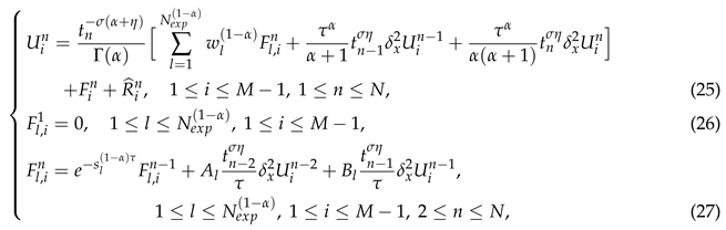
Now, we present a fast difference scheme for the problem (1)-(3). Similar to the treatment of the direct difference scheme, applying (20) in temporal direction, we get where there exists a constant $c_2$ such that

$$|{\widehat{R}}_i^n|\le c_2({\tau }^2+h^2+ϵ),1\le i\le M-1,1\le n\le N.$$

(28)

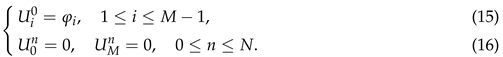
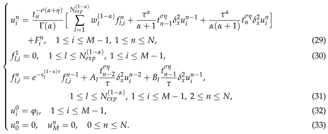
Omitting the small term ${\widehat{R}}_i^n$ in (Section 3.2), replacing the grid functions $\{U_i^n,F_{l,i}^n\}$ by their numerical approximations $\{u_i^n,f_{l,i}^n\}$ and noticing the initial-boundary value conditions (15)-(16), we arrive at following fast difference scheme

4. Numerical Analysis

This section provides numerical validation demonstrating the effectiveness of our novel discretization framework for Erdélyi-Kober integration operator. Through a detailed comparative analysis of CPU time between the direct difference scheme (17)-(19) and the fast difference scheme (29)-(33), our computational experiments reveal that the accelerated algorithm significantly enhances computational efficiency with complexity reduced from $O\left(N^2\right)$ to $O(NlogN)$. The absolute tolerance error $ϵ={10}^{-12}$ is adopted in our numerical simulations.

Example 1. 

We choose the exact solution of the problem (5) to be $u(x,t)=t^{\alpha +2-\sigma \eta }sinx.$ The right hand side function is determined by the exact solution as follows:

$$F(x,t)=\left[1+{\displaystyle \frac{\Gamma (1+\frac{\alpha +2}{\sigma })}{\Gamma (\alpha +1+\frac{\alpha +2}{\sigma })}}\right]t^{\alpha +2-\sigma \eta }sinx.$$

Let the finial time $T=1.$ The spatial domain $\Omega =(0,2\pi ).$ To examine the accuracy and efficiency of the difference schemes, the $L^2$-norm error

$$E(h,\tau )=\underset{0\le n\le N}{max}\parallel U^n-u^n\parallel$$

is recorded in each run and the experimental orders are evaluated by

$$R_{\tau }={log}_2\left({\displaystyle \frac{E(h,2\tau )}{E(h,\tau )}}\right),R_h={log}_2\left({\displaystyle \frac{E(2h,\tau )}{E(h,\tau )}}\right).$$

The accuracy tests are performed by taking the parameter $\eta =0.2,\sigma =0.9$ for three fractional orders $\alpha =0.1,0.5$ and $0.9.$ The error analyses for both the direct and accelerated difference schemes establish an asymptotic convergence order of $O({\tau }^2+h^2)$ with the theoretical upper bounds demonstrating remarkable agreement with empirical convergence rates observed in our numerical simulations.

Table 1 shows the numerical accuracy and CPU time of two difference schemes in time. To isolate temporal errors, we employ a refined spatial discretization with $h=\pi /2500.$ The numerical verification results confirm second-order temporal accuracy, demonstrating remarkable agreement between empirical convergence rates and theoretical predictions.

Next, we turn to test the numerical accuracy and corresponding CPU time of two difference schemes in space. Fix a fine temporal step size $\tau =1/20000$ such that the spatial errors dominate the temporal errors. Table 2 records the numerical results of two difference schemes when solving the example for different $\alpha .$ One can observe that convergence orders of two difference schemes are good agreement with theoretical results. Furthermore, the computational cost of the direct difference scheme is largely higher than that of the fast difference scheme, which also reflects from the side the high efficiency of the fast algorithm.

5. Concluding Remarks

This paper presented two temporal second-order difference schemes for solving time-fractional diffusion equations involving the Caputo-type Erdélyi-Kober operator, accompanied by rigorous error estimation. While a complete theoretical framework for the difference schemes remains to be developed, we nevertheless establish critical properties of the temporal L1-type formula’s coefficients. Domain knowledge suggests that these coefficient properties constitute fundamental prerequisites for rigorous stability and convergence analyses in such fractional calculus contexts. Consequently, the present work establishes a methodological foundation that may inform subsequent theoretical investigations. The numerical validation section conclusively demonstrates the theoretical convergence rates through systematic implementation.

References

- Al-Musalhi, F., Al-Salti, N., Karimov, E. Initial boundary value problems for a fractional differential equation with hyper-Bessel operator. Fract. Calc. Appl. Anal., 21 (2018), pp. 200-219.
- de Pablo, A., Quirós, F., Rodríguez, A., Vázquez, J. L. A fractional porous medium equation. Adv. Math., 226 (2011), pp. 1378-1409.
- Erdélyi, A., Kober, H. Some remarks on Hankel transforms. Quart. J. Math. Oxford Ser., 11 (1940), pp. 212-221.
- Jiang, S. D., Zhang, J. W., Zhang, Q., Zhang, Z. M. Fast evaluation of the Caputo fractional derivative and its applications to fractional diffusion equations. Commun. Comput. Phys., 21 (2017), pp. 650-678.
- Jin, B. T., Li, B. Y., Zhou, Z. An analysis of the Crank-Nicolson method for subdiffusion. IMA J. Numer. Anal., 38 (2018), pp. 518-541.
- Kiryakova, V. S. Generalized fractional calculus and applications. CRC Press, 1993.
- Li, C. P., Cai, M. Theory and numerical approximations of fractional integrals and derivatives. Society for Industrial and Applied Mathematics (SIAM), Philadelphia, PA, (2020), pp. xiii+312.
- Lin, Y. M., Xu, C. J. Finite difference/spectral approximations for the time-fractional diffusion equation. J. Comput. Phys., 225 (2007), pp. 1533-1552.
- Luchko, Y., Trujillo, J. J. Caputo-type modification of the Erdélyi-Kober fractional derivative. Fract. Calc. Appl. Anal., 10 (2007), pp. 249-267.
- Mainardi, F. Fractional calculus and waves in linear viscoelasticity. Imperial College Press, London, (2010), pp. xx+347.
- Metzler, R., Klafter, J. The random walk’s guide to anomalous diffusion: a fractional dynamics approach. Phys. Rep., 339 (2000), pp. 77.
- Metzler, R., Klafter, J. Accelerating Brownian motion: A fractional dynamics approach to fast diffusion. Europhys. Lett., 51 (2000), pp. 492-498.
- Mura, A., Taqqu, M. S., Mainardi, F. Non-Markovian diffusion equations and processes: analysis and simulations. Phys. A, 387 (2008), pp. 5033-5064.
- Nigmatullin, R. R. To the theoretical explanation of the “Universal Response”. Physica B, 123 (1984), pp. 739-745.
- Odibat, Z., Baleanu, D. On a new modification of the Erdélyi-Kober fractional derivative. Fractal Fract., 5 (2021), pp. 121.
- Pagnini, G. Erdélyi-Kober fractional diffusion. Fract. Calc. Appl. Anal., 15 (2012), pp. 117-127.
- Płociniczak, ł. Approximation of the Erdélyi-Kober operator with application to the time-fractional porous medium equation. SIAM J. Appl. Math., 74 (2014), pp. 1219-1237.
- Płociniczak, łukasz, Świtała, Mateusz. Numerical scheme for Erdélyi-Kober fractional diffusion equation using Galerkin-Hermite method. Fract. Calc. Appl. Anal., 25 (2022), pp. 1651-1687.
- Płociniczak, ł., Sobieszek, S. Numerical schemes for integro-differential equations with Erdélyi-Kober fractional operator. Numer. Algorithms, 76 (2017), pp. 125-150.
- Sneddon, I. N. The use in mathematical analysis of Erdélyi -Kober operators and some of their applications. Fract. Calc. Appl., 457 (1975), pp. 37-79.
- Tang, J. H. Analysis and Calculation of Erdélyi-Kober Fractional Differential Equations(Doctoral thesis), Shanghai University, 2022.
- Thongsalee, N., Ntouyas, S. K., Tariboon, J. Nonlinear Riemann-Liouville fractional differential equations with nonlocal Erdélyi-Kober fractional integral conditions. Fract. Calc. Appl. Anal., 19 (2016), pp. 480-497.
- Wang, J. R., Dong, X. W., Zhou, Y. Analysis of nonlinear integral equations with Erdélyi-Kober fractional operator. Commun. Nonlinear Sci. Numer. Simul., 17 (2012), pp. 3129-3139.
- Zhang, K. Q. Applications of Erdélyi-Kober fractional integral for solving time-fractional Tricomi-Keldysh type equation. Fract. Calc. Appl. Anal., 23 (2020), pp. 1381-1400.
- Zhang, K. Q. Existence and uniqueness of analytical solution of time-fractional Black-Scholes type equation involving hyper-Bessel operator. Math. Methods Appl. Sci., 44 (2021), pp. 6164-6177.
- Zhang, Y. N., Sun, Z. Z., Wu, H. W. Error estimates of Crank-Nicolson-type difference schemes for the subdiffusion equation. SIAM J. Numer. Anal., 49 (2011), pp. 2302-2322.