
Submitted:
05 October 2024
Posted:
08 October 2024
You are already at the latest version
Abstract
An innovative approach is utilized in this paper to solve the Fractional Fokker–Planck–Levy (FFPL) equation. A hybrid technique is designed by combining the finite difference method (FDM), Adams numerical technique, and physics-informed neural network (PINN) architecture, namely, the FDM-APINN, to solve the fractional Fokker‒Planck‒Levy (FFPL) equation numerically. Two scenarios of the FFPL equation are considered by varying the value of α (i.e., 1.75,1.85). Moreover, three cases of each scenario are numerically studied for different discretized domains with 100,200 and 500 points in x∈[-1,1] and t∈[0,1]. For the FFPL equation, solutions are obtained via the FDM-APINN technique via 1000,2000, and 5000 iterations. The errors, loss function graphs, and statistical tables are presented to validate our claim that the FDM-APINN is a better alternative intelligent technique for handling fractional-order partial differential equations with complex terms. FDM-APINN can be extended by using nongradient-based bioinspired computing for higher-order fractional partial differential equations.
Keywords:
Fractional Fokker‒Planck‒Levy Equation
; Physics-Informed Neural Networks (PINNs)
; Finite Difference Method (FDM)
; Adams Numerical Technique
; Hybrid Numerical Method
; Fractional Partial Differential Eq
1. Introduction
The fractional Fokker–Planck (FFP) equation, also known as the Fokker–Planck Levy (FPL) equation, is the generalization of the traditional Fokker–Planck (FP) equation, which includes Levy processes, such as heavy-tailed distributions or leaps. The Fractional Fokker–Planck Levy (FFPL) equation is applied in finance, ecology, and physics for anomalous diffusion in complex systems, abrupt, long-range movements in animal movement patterns, and jumps or heavy tails in the underlying asset. The traditional Fokker–Planck equation describes the time evolution of a particle's probability density function of velocity under the influence of forces and Gaussian white noise. Gaussian processes, however, cannot fully explain the leaps and heavy tails observed in a wide range of physical and economic phenomena. A more suitable mathematical framework for such situations is provided by Levy processes, which comprise a larger class of stochastic processes defined by stable distributions and leaps. The fractional derivative causes nonlocality, which requires specialized numerical techniques that are capable of handling integral terms efficiently. By adding fractional derivatives, the Fractional Fokker Levy Planck Levy (FFPL) equation extends the traditional Fokker Planck (FP) equation, which is capable of modelling these jump-like, nonlocal dynamics. Recently, fractional calculus has improved financial system modelling by providing a more complete understanding of asset dynamics. Fractional calculus extends integration and differentiation to fractional orders, empowering the introduction of memory and long-range dependencies in mathematical models [1,2,3]. While conventional numerical techniques are excellent for solving classic PDEs, they may not handle fractional derivatives effectively. Scholars such as Chen et al. [4] and Nikan et al. [5] have attempted to improve conventional numerical techniques by adopting mesh-free approaches such as the radial basis function (RBF) method to solve fractional PDEs. However, the RBF technique complicates the selection of the basis function.
Solving the FFPL equation numerically is challenging because both the large discrete changes caused by the jump term and the small-scale behaviour driven by the diffusion term are needed. The FFPL equation of interest in this paper poses additional important challenges, where classical grid-based approaches fail because of the increase in computational requirements with the nonlocality of the partial differential equation (PDE), making them impractical. Physics-informed neural networks (PINNs) [6] are currently popular in solving partial differential equations (PDEs) because neural networks have high universal approximation characteristics [7], robust optimization [8], meshless plus grid-free training, and generalization capacities [9].
The PINN is a promising strategy for solving large PDEs because it incorporates physical rules and constraints directly into the learning process [10,11]. The PINN technique uses fractional derivatives in the governing partial differential equation (PDE) to obtain an acceptable approximation of the solution. The PINN design includes a loss function that enforces the differential equation, boundary, and initial conditions, resulting in precise solutions even with insufficient input. The PINN algorithm integrates the fractional derivative into the FFPL equation and uses neural networks to acquire the basic solution. The PINN ensures that the solution has physical stability and responds to real-world financial complications. Several studies, including those of Ibrahim et al. [12,13], Jamshaid et al. [14], and Lou et al. [15], have employed this approach to solve PDEs instead of other approaches. High-dimensional PINNs [16,17] use automatic differentiation to calculate integer-order derivatives. Compared with automatic differentiation, the FDM-APINN is faster and consistently results in fewer errors [18]. A PDE solver PINN technique is generated by [19] and inspired by the FDM-APINN, which shows that the method consistently results in minimal errors. Automatic differentiation and FDM-APINN libraries currently do not cover fractional-order derivatives. Approximating the fractional Laplacian still remains a significant challenge. For the approximation of the fractional Laplacian, we used the finite difference method (FDM) in this manuscript. Fractional FPL equations provide a challenge for both classical and novel methodologies, such as PINNs.
We introduce a special type of FDM-APINN technique to solve the fractional FPL equation. The loss function used in this technique considers not only the mean squared error (MSE) between actual and predicted data (data loss) but also physics-based loss. This additional loss element requires the neural network to follow the physical principles specified by the FFPL equation. The fractional Laplacian is also under consideration in this technique. The fractional Laplacian is an essential component in fractional PDEs, distinguishing them from classical PDEs. The FDM method is used for the approximation of the fractional Laplacian and then utilized in the PINN. This technique employs automatic differentiation to produce the gradients required for calculating the physics-based loss. This enables the FDM-APINN to handle the complex derivatives found in the FFPL equation. Furthermore, the physics loss is also computed. The neural network predictions are guaranteed to satisfy the FFPL equation via physics loss, which makes the model physics-informed. Therefore, the proposed technique is unique and efficient.
1.1. Related Work
FPL and FP equations are frequently encountered in statistical mechanics, and their large dimensionality presents notable difficulties for conventional analytical techniques such as finite difference [20,21]. However, physics-informed neural networks (PINNs), which are machine learning techniques, present a promising mesh-free approach that seamlessly integrates observational data. PINNs were used in Chen et al.'s research [22] to solve forward and inverse problems related to the Fokker–Planck–Levy equations. Zhang et al. [23] addressed FP equations involving sparse data via deep KD-tree techniques. Similarly, deep learning was used by Zhai et al. [24] and Wang et al. [25] to solve steady-state FP equations. Moreover, Lu et al. [26] concentrated on employing normalizing flows to learn high-dimensional probability densities modelled by FP equations. Furthermore, normalization flow approaches were used for FP equations by Feng et al. [27] and Guo et al. [28]. and Tang et al. [29] presented an adaptive deep density approximating technique for steady-state FP equations based on normalizing flows, and for FP equations, Hu et al. [30] presented a score-based SDE solution. This paper introduces an innovative technique that combines the FDM, ADAMS, and PINN to solve the fractional Fokker–Planck-Levy (FFPL) equation.
1.2. Paper Highlights
- ➢
- An innovative approach is utilized in this paper to solve the Fractional Fokker–Planck–Levy (FFPL) equation. The equation contains the Levy noise and fractional Laplacian, making the equation computationally complex.
- ➢
- A hybrid technique is designed by combining the finite difference method (FDM), Adams numerical technique, and physics-informed neural network (PINN) architecture, namely, the FDM-APINN, to solve the fractional Fokker‒Planck‒Levy (FFPL) equation numerically.
- ➢
- Related work on solving partial differential equations (PDEs) and fractional partial differential equations (FPDEs) is discussed.
- ➢
- The fractional Fokker–Planck-Levy (FFPL) equation is solved numerically via the proposed technique.
- ➢
- The manuscript is categorized into two main scenarios by varying the value of the fractional order parameter . The equation is solved for the two values of , i.e., ().
- ➢
- The loss values given for each case can be visualized in the tables. The loss values are very minimal, ranging between and , indicating the precision of the proposed technique.
- ➢
- All the solutions of the proposed technique are compared with those of the score-fPINN technique, which is a well-known technique for solving fractional differential equations.
- ➢
- The residual error graph and tables show the errors between both techniques. The errors range between and . The small error indicates the validity of our proposed technique.
- ➢
- Furthermore, loss and error graphs have been added to the manuscript to explore the proposed technique further. The histogram graph shows the consistency of the proposed technique.
- ➢
- All the results presented in the tables and graphs indicate that the proposed technique is a state-of-the-art technique that is robust.
2. Defining the Problem
Stochastic differential equations are commonly used to represent the time development of dynamic systems in fields such as natural sciences, engineering, economics, and statistics [31,32,33]. The density is obtained by solving the Fokker–Planck equation (FPE), which may be written as [34]:
where represents the value of the density at time , is a tensor called a diffusion matrix, and is a vector field known as the drift function. If the -stable Levy noise term is introduced to eq (1) and is replaced as , then the Fractional Fokker–Planck Levy (FFPL) equation is given as:
where
- , is defined as
- ➢
- represents the diffusion term; in this problem, it is taken as the identity matrix.
- ➢
- where is the Levy noise.
- ➢
- is the order of the fractional Laplacian, where .
- ➢
- represents the fractional Laplacian operator of order .
Given the constants and definitions mentioned above, the equation's full form can be expressed as follows.
here,
- ➢
- is the drift term.
- ➢
- is the diffusion term
There are several specific distributions regarding values:
- If , then it is a Gaussian distribution.
- If , then it is a Cauchy distribution.
- If , then it is a Holtsmark distribution, whose PDF is a hypergeometric function.
Fractional Laplacian
The term represents the fractional Laplacian term. This term is beneficial for solving fractional equations involving fractional derivatives, such as the FFPL solved in this paper. The fractional Laplacian used in this paper is calculated through the finite difference method (FDM).
The fractional Laplacian is a nonlocal operator that generalizes the classical Laplacian to fractional powers, with generally between and . The fractional Laplacian can be defined in various ways, but one of the most frequent uses is the spectral method or an integral representation, which reflects its nonlocal character.
In , the fractional Laplacian through the FDM of can be defined as follows:
where
- where represents the fractional order of the Laplacian.
- is the dimension.
The domain is divided into grid points with regular spacing .
where
is the length of the domain of ().
The fractional Laplacian is represented in matrix form. The matrix is designed to approximate the fractional Laplacian operator. The primary goal is to simulate the fractional Laplacian with a discrete sum over the grid points. The discrete fractional Laplacian is represented in matrix form as:
where , defined as
The matrix element reflects the contribution from point to the fractional Laplacian at . The contribution is inversely proportional to the distance. is raised to the power . The fraction is scaled by to accommodate the integral's discretization. The diagonal element ensures that the sum of all the elements in each matrix row is zero. The Laplacian's conservation property requires that the total flux into a point be zero if is constant. The proposed flexible technique can be used in different boundary conditions and domains.
3. Proposed Methodology
Since the beginning, the PINN has undergone extensive study to improve its ability to solve complicated problems in numerous fields. Several researchers have focused on implementing advanced algorithms in PINNs, such as adaptive sampling approaches [35,36,37,38,39], adaptive activation functions [40,41,42], dynamic weighting for loss terms [43,44,45], and sequential training [46,47]. New architectural frameworks have been developed to address specific problems more efficiently. Some notable examples include the conservative PINN (cPINN) [48], parareal physics-informed neural network (PPINN) [49], Bayesian PINN (BPINN) [50], extended PINN (XPINN) [51,52], physics-informed generative adversarial network (PI-GAN) [53], and gradient-enhanced neural network (gPINN) [54,55,56]. Although PINNs have a promising future, they have yet to be applied to some PDEs. More importantly, fractional problems, such as the Fractional Fokker Planck Levy (FFPL) equation discussed in this paper, are challenging to solve. The FDM-APINN technique is used to solve the FFPL equation.
The proposed technique has two input values, i.e., and t. There are two fully connected hidden layers, each having neurons. The ReLU activation function is used in the proposed approach. The deep learning phenomenon is used. The optimizer used is the Adam optimizer. The proposed technique evaluates the trained network on the test data, and the predicted solutions are obtained from the results. The loss values are obtained as the sum of two types of loss. One is data loss, and the second is physics loss. To calculate the physics loss, the fractional Laplacian and all the gradients are calculated, ensuring that all the operations comply with the FFPL equation.
The general working phenomenon of the proposed technique is shown in Figure 1. In Figure 1, the inputs are associated with hidden layers consisting of hidden neurons. After performing some hidden calculations, the output layer is obtained. After that, the loss is calculated as the sum of the data loss and physics loss. The minimum loss obtained means that the technique converges to the optimal solutions.
3.1. Loss Function
The loss function consists of two elements: data loss and physical loss. This ensures that the trained neural network matches the training data and follows the physical rules stated in the Fractional Fokker Planck Levy (FFPL) equation.
3.1.1. Data Loss
Data loss determines how closely the neural network's predictions correspond to the training data. It is the mean squared error (MSE) between the actual predicted values.
where represents the sample of training data, represents the predicted solution at , and is the actual solution at .
3.1.2. Errors
The mathematical model under consideration in is given as
The errors for the given FFPL equation are given as
3.1.3. Physics Loss
The physical loss for the proposed technique is defined as the mean square of the
3.1.4. Total Loss
The total loss for the proposed technique is calculated as
In short, the total loss function combines data loss with physics loss. The proposed technique influences the rule of neural networks to predict data and ensures that the solution is physically meaningful.
The network contains an input layer for and , two hidden layers with ReLU activation and an output layer for . is the number of neurons attached to each layer. Synthetic data have been generated to mimic while training the network. Different physical parameters are used in the mathematical model. The values of the parameters of the FFPL equation are defined, including (fractional order), , and the functions and . The network is trained via mini-batches across several epochs. The loss function combines data loss with physics loss. Gradients are calculated and utilized to adjust network settings via the Adam optimizer. The overall loss is calculated by adding data loss and physics loss. During training, the network is assessed on test data to predict , which is then visualized. This strategy integrates data-driven machine learning with the physical constraints of the FFPL equation, utilizing the strengths of each approach to discover a solution. One of the primary novelties here is the incorporation of physics loss into neural network training, which ensures that the acquired solution follows basic physical principles.
3.2. Optimizer
The optimizer used in the proposed technique is the Adam optimizer. Adam is the short form of adaptive moment estimation. It is an optimization algorithm that integrates the benefits of two widely used optimization algorithms, AdaGrad and RMSProp.
Working of the Adam optimizer
Set the time step () to , the moment vector to , and the moment vector to . Define the hyperparameters. Then, the gradients are computed by
update the biassed moment value by
update the biassed moment value by
compute the bias-corrected moment estimates
compute the bias-corrected moment estimates
update the parameters by
where
- ➢
- is the time step.
- ➢
- represents the parameters at time step .
- ➢
- is the gradient of the objective function w.r.t. at time step .
- ➢
- is the 1st moment vector (mean of the gradients).
- ➢
- is the 2nd moment vector (uncentered variance of the gradients).
- ➢
- is the learning rate.
- ➢
- are the exponential decay rates for the moment estimates.
- ➢
- where is a small constant for numerical stability.
The FDM-APINN technique is used to solve the given mathematical model in the manuscript. The working phenomenon of the proposed architecture is explained in the pseudocode given in Algorithm 1:
The flow chart of the paper is given in Figure 2. All the working phenomena of the proposed technique in the manuscript are given in the flow chart of the paper in Figure 2. The flow chart shows the procedure followed in the manuscript.
| Algorithm 1: Pseudocode representing all the working procedures of FDM-APINN | ||||||
| Starting FDM-APINN | ||||||
| 1 | Defining Neural Networks | |||||
| 2 | Select number of input layers as 2 | |||||
| 3 | 50 is the number of hidden neurons selected | |||||
| 4 | Parameters setting | |||||
| 5 | Select the number of iterations and learning rate | |||||
| 6 | Set values of physical parameters and | |||||
| 7 | Generate training data | |||||
| 8 | Grid points creation of and | |||||
| 9 | Set the initial condition | |||||
| 10 | Training Loop | |||||
| 11 | Select a mini-batch sample | |||||
| 12 | Prepare input data and convert it to a deep-learning array | |||||
| 13 | Compute gradients and loss functions | |||||
| 14 | Use the Adam optimizer to update the network | |||||
| 15 | Display loss | |||||
| 16 | Evaluation of the network | |||||
| 17 | Predict and plot using test data | |||||
| 18 | Calculate the targeted functions | |||||
| 19 | Compute the derivatives . | |||||
| 20 | Compute the function of fraction Laplacian using FDM | |||||
| 21 | Compute the data loss function | |||||
| 22 | Compute the physics loss functions | |||||
| 23 | Compute gradients and total loss | |||||
| End of the algorithm FDM-APNN | ||||||
The FDM-APINN methodology is used in this paper to solve the FFPL equation. The neural networks used in the PINNs are trained several times to explore the technique's efficiency thoroughly, while the fractional Laplacian term is approximated through the FDM. The paper is divided into two different scenarios by varying the value of the fractional order parameter . For each value of , the domain of the inputs and is distributed to and different points. For each distribution, and iterations are performed. We used the outputs of the score-fPINN technique as a reference solution to validate our results. Different loss and error graphs are given for each number of iterations to evaluate the technique's validity and accuracy. From all the graphs, it is clear that the proposed technique is state-of-the-art with great accuracy. Moreover, different tables are also provided in the paper for further evaluation of the proposed method. The MATLAB code of the designed methodology is as follows:
https://github.com/ffazal1/FDM_APINN.git whenever our paper is accepted for publication.
4. Results and Discussion
This section presents all the results of the proposed technique, i.e., the FDM-APINN technique. Two scenarios are created by varying the value of the fractional order parameter . For each value of the fractional parameter , the domain of and is distributed to and different equidistant points. Then, for each distribution, and iterations are performed. All the results obtained are given in this section. The residual error tables and graphs presented in the manuscript are the errors between the outputs of the proposed technique (FDM-APINN) and the reference technique (score-fPINN). Graphical and statistical illustrations are discussed in detail in this section.
Table 1 shows the pattern of the paper. In the first column of Table 1, the value of the fractional order varies. The mathematical model is solved for each value, and the results are obtained via the FDM-APINN in the MATLAB window. In the first scenario, the mathematical model is solved for the value of the fractional order . The second column of Table 1 shows the distribution of points taken between the domains of and . We distributed the domain of (i.e., ) into different equidistant points and solved the FFPL equation. Similarly, the domain of is distributed to different equidistant points to obtain the solutions about different points. The row of the column shows the distribution of the domain to points. We distributed the domain of into different equidistant points and solved the FFPL equation.
Similarly, the domain of is distributed to different different equidistant points to obtain solutions about different points. Similarly, the same procedure is repeated for the distribution of the domains into points, as shown in the row of the column. After that, we trained the FDM-APINN for iterations for points and obtained the results. Then, the FDM-APINN is run for iterations for the same distribution, i.e., points distribution. In the final round, iterations are performed to obtain the solutions at different points. In the same manner, and iterations are performed to obtain the results for and points for the same value of . All the procedures discussed above are repeated for the values of the fractional order and .
4.1. Scenario 1
This section discusses all the results obtained for the first scenario. In the first scenario, the value of the fractional order parameter is set to . Then, three cases are formed for the first scenario by dividing the domains of and into and different points. The mathematical model is solved for each case by performing and iterations. The graphical and tabular results of the first scenario are discussed in this section of the manuscript.
Table 2 shows the average loss for the value of the fractional order . The 1st column of the table shows the and point distributions between the domains of and . For points, and iterations are performed for each distribution individually, as given in the column of Table 2. The column of Table 2 shows the average loss obtained after and iterations. Table 2 shows that the average loss obtained in this paper is minimal, which confirms the validity of our proposed technique. Each value of the average loss is in the range of and . This finding indicates that our proposed technique is highly consistent.
Figure 3 shows a graphical illustration of the solution graphs of the Fractional Fokker Planck Levy (FFPL) equation. From Figure 3, the density is the maximum at the mean and decreases as we move towards the extreme points. The maximum value of the density is 1. Solution graphs obtained after solving the Fractional Fokker–Planck Levy (FFPL) equation for 100, 200, and 500 point distributions. Five thousand iterations are performed for each case.
After performing 1000, 2000, and 5000 iterations, the residual error values are obtained, as shown in Table 3. These values are obtained by taking different points between the domains of and , while the value of the fractional parameter is . Table 3 shows the residual error values between the solutions of the proposed technique and the score-fPINN. The column of the table shows the input values. These values are obtained for the distribution of the domains of and into different points. The column of the table shows the input values. The column represents the residual error values after iterations are performed. Similarly, columns and show the residual error values after performing and iterations, respectively. The table clearly shows that the residual errors are close to , ranging between and , which demonstrates that the proposed technique is a state-of-the-art, accurate, and valid technique.
Figure 4(a) shows the graph of the loss values. Figure 4(a) shows the iterations for the -point distribution of the domain of and , while the value of the fractional order is . The x-axis of the graph represents the number of iterations, and the y-axis represents the loss values. From Figure 4(a), the loss value decreases and approaches zero as the number of iterations increases, which shows that we are approaching the optimal solutions. At the start, the loss value is not close to zero, but at the 1000th iteration, the loss value is very close to zero. This means that as we approach the 1000th iteration, the solutions approach their optimal values. Figure 4(b) shows the graph of the residual error values between the proposed technique and the score-fPINN technique. Figure 4(b) shows the errors obtained during the iterations for the point distributions of the domains of and . Figure 4(b) shows the values of , , and the corresponding errors. All points lie between and , which shows that minimal residual errors are present. These minimal residual errors indicate the accuracy and consistency of the proposed technique.
The graph of the loss values of the proposed technique is shown in Figure 4(c). Figure 4(c) shows the loss values for iterations of the -point distribution of the domains of and , where the value of the fractional order parameter is . The x-axis of the graph represents the number of iterations, and the y-axis shows the loss values. Figure 4(c) shows that the loss value decreases and approaches zero as the number of iterations increases. This shows that we are approaching the optimal solutions. At the start of the iterations, the loss value is not close to zero, but after iterations, the loss values oscillate around . As we approach iterations, the loss value approaches . This means that as we approach the iteration, the solutions approach their best optimal values. Figure 4(d) shows the graph of the residual error values. Figure 4(d) shows the errors obtained during the iterations for the point distributions of the domains of and . Figure 4(d) shows the values of and the corresponding errors. We take points to observe the residual errors. Figure 4(d) shows that the errors are very close to zero, indicating the accuracy and consistency of our proposed technique.
Figure 4(e) shows the histogram graph for the loss values. Figure 4(e) shows the loss values for iterations of the -point distribution of the domains of and , where the value of the fractional order parameter is . The x-axis of the graph represents the loss values, and the y-axis of the graph represents the number of iterations. The graph shows that at approximately iterations, the loss values are the same and very close to . This finding indicates that our proposed technique is highly consistent and reliable. Figure 4(f) shows the graph of the residual error values. Figure 4(f) shows the errors obtained during the iterations for the point distributions of the domains of and . Figure 4(f) shows the , , and residual error values. All the error values lie between and . Figure 4(f) shows that the errors are very close to zero, indicating the accuracy and consistency of our proposed technique.
Table 4 shows the residual error values between the actual and predicted values. The domains of and are divided into different equidistant points. The fractional order is . In Table 4, the column shows the input values, whereas the column represents the input values. The and columns show the residual errors. The column shows the residual error values after performing iterations. Similarly, after iterations, the residual errors obtained are shown in the column. The column shows the residual error values after performing iterations. All the values of the residual errors are minimal, confirming the validity of the technique. Furthermore, the residual error values are also very close to each other, indicating the consistency of the proposed technique. The residual error values range from to , which is very good for fractional problems.
Figure 5(a) shows the graph for the loss values. Figure 5(a) shows the loss values for iterations of the -point distribution of the domains of and , where the value of the fractional order parameter is . The x-axis of the graph represents the number of iterations, and the y-axis of the graph represents the loss values. Figure 5(a) shows that as the number of iterations increases, the loss value decreases and approaches zero. This shows that we are approaching the optimal solutions. At the start of the iterations, the loss value is not close to zero, but after iterations, the loss value approaches . As we reach the iterations, the loss value approaches . Figure 5(b) shows the graph of the residual error values in the output of the proposed technique and the score-fPINN technique. Figure 5(b) shows the errors obtained during the iterations for the point distributions of the domains of and . Figure 5(b) shows the values of , , and the corresponding errors. All points have very minimal residual error values, as shown in Figure 5(b), indicating the accuracy and consistency of our proposed technique.
The loss value graph is shown in Figure 5(c). The graph shown in Figure 5(c) is for the loss values obtained after approximately iterations by taking different points between the domains of and . The value of the fractional parameter is . The iterations are represented through the -axis, while the loss values are shown on the y-axis of Figure 5(c). As the number of iterations increases, the loss value decreases and approaches zero, indicating that we are approaching the optimal solutions. At the beginning of the graph, the loss values are not close to zero, whereas at the end of the graph, the values are close to zero. Additionally, at the start of the graph, the loss values vary, but after iterations, the graph becomes smooth, showing that the solutions obtained through the proposed technique approach optimal solutions. The error values are shown in Figure 5(d). These errors are obtained through different points between the domains of and . iterations are performed to obtain these errors. We take 11 different points from the points. Clearly, the errors are very close to , confirming the validity and consistency of the proposed technique.
The graph shown in Figure 5(e) is for the loss values obtained after approximately iterations by taking different points between the domains of and . The value of the fractional parameter is . The iterations are represented through the -axis, while the loss values are shown on the -axis of Figure 5(e). In approximately iterations, the loss values overlap each other. The histogram in Figure 5(e) shows the consistency of our proposed technique. The residual error values are shown in Figure 5(f). These are the errors obtained through different points between the domains of and . These residual errors were obtained after iterations. Clearly, the errors are very close to , confirming the validity and consistency of the proposed technique.
Table 5 shows the residual error values between the actual and predicted values. The domains of and are divided into different equidistant points. The fractional order is . The table column shows the input values, whereas the column represents the input values. The and columns show the residual errors. The column shows the residual error values after performing iterations. Similarly, after 2000 iterations, the residual errors obtained are demonstrated by the column. Moreover, the column shows the residual error values after performing iterations. All the values of the residual errors are minimal, confirming the technique's validity. Furthermore, the residual error values are also very close to each other, confirming the consistency of the proposed technique. The residual error values range from to , which is very good for fractional problems.
Figure 6(a) shows the graph for the loss values. Figure 6(a) shows the loss values for iterations of the -point distribution of the domains of and , where the value of the fractional order parameter is . The -axis of the graph represents the number of iterations, and the -axis of the graph represents the loss values. Figure 6(a) shows that the loss value decreases and approaches zero as the number of iterations increases. This indicates that the proposed technique converges toward the optimal solutions. At the start of the iterations, the loss value is not close to zero, but at the iteration, the loss value approaches . As we reach the iterations, the loss value approaches . Figure 6(b) shows the graph of the residual error values. Figure 6(b) shows the errors obtained during the iterations for the point distributions of the domains of and . Figure 6(b) shows the , , and error values. All the error values range from to . In Figure 5(b), the errors are very close to zero, indicating the accuracy and consistency of our proposed technique.
The loss value graph is shown in Figure 6(c). The graph shown in Figure 6(c) is for the loss values obtained after approximately iterations by taking different points between the domains of and . The value of the fractional parameter is . The iterations are represented through the -axis, while the loss values are shown on the -axis of Figure 6(c). As the number of iterations increases, the loss value decreases and approaches zero, indicating that the optimal solutions are obtained. At the beginning of the graph, the loss values are not close to zero, whereas at the end, the values are close to zero. Additionally, at the start of the graph, the loss values vary, but after 1000 iterations, the graph becomes smooth, showing that the solutions obtained through the proposed technique approach optimal solutions. The error values are shown in Figure 6(d). These errors were obtained through different points between the domains of and . iterations are performed to obtain these errors. We take different points from the points. The errors are very close to , confirming the validity and consistency of the proposed technique.
Figure 6(e) shows the graph for the loss values. Figure 6(f) shows the loss values for iterations of the -point distribution of the domains of and , where the value of the fractional order parameter is . The -axis of the graph represents the loss values, and the -axis of the graph represents the number of iterations. The histogram graph shows the consistency of the proposed technique. The graph is given for iterations. Out of iterations, approximately iterations, the loss values overlap. Figure 6(f) shows the graph of the residual error values. Figure 6(f) shows the errors obtained during the iterations for the point distributions of the domains of and . Figure 6(f) shows the values of , and the corresponding errors. Figure 6(f) shows that the errors are very close to zero for all points, indicating the accuracy and consistency of our proposed technique.
4.2. Scenario2
In this section, all the results obtained for the second scenario are discussed. In the second scenario, the fractional order parameter alpha value is . Three cases are formed for the second scenario by dividing the domains of and into and different points. The mathematical model is solved for each case by performing and iterations. All the graphical and tabular results of the second scenario are discussed in this section of the manuscript.
Table 6 shows the average loss for the value of the fractional order. . The column of Table 6 shows the and point distributions between the domains of and . For points,
and iterations are performed for each distribution individually, as given in the column of Table 6. The column of Table 6 shows the average loss obtained after and iterations. The column of Table 6 shows that the average loss obtained in this paper is minimal, which shows the validity of our technique. Each value of the average loss ranges between and . This shows the consistency of our technique.
Figure 7 shows a graphical illustration of the solution graphs of the Fractional Fokker Planck Levy (FFPL) equation. From Figure 7, the density is the maximum at the mean and decreases as we move towards the extreme points. The maximum value of the density is 1. These are the solutions obtained after performing iterations for the and distributions, respectively.
After performing and iterations, respectively. The residual error values are obtained, as shown in Table 7. These values are obtained by taking different points between the domains of and , while the value of the fractional parameter is . Table 7 shows the residual errors obtained from the proposed technique. The column of the table shows the input values. These values are obtained for the distribution of the domains of and into different points. The column of the table shows the input values. The column of the table represents the residual error values after iterations are performed. Similarly, the and columns show the residual error values after performing and iterations, respectively. Table 7 clearly shows that the residual errors are close to , ranging between and , which demonstrates that the proposed technique is a state-of-the-art, accurate, and valid technique.
Figure 8(a) shows the graph for the loss values. Figure 8(a) shows the loss values for iterations of the -point distribution of the domains of and , where the value of the fractional order parameter is . The -axis of the graph represents the number of iterations, and the -axis of the graph represents the loss values. Figure 8(a) shows that the loss value decreases and approaches zero as the number of iterations increases. This indicates that the proposed technique converges toward the optimal solutions. At the start of the iterations, the loss value is not close to zero, but at the iteration, the loss value approaches . As we reach the iterations, the loss value approaches . Figure 8(b) shows the graph of the residual error values. Figure 8(b) shows the errors obtained during the iterations for the point distributions of the domains of and . Figure 8(b) shows the values of , , and the corresponding errors. All the error values range from to . Figure 8(b) shows that the errors are very close to zero, indicating the accuracy and consistency of our proposed technique.
The loss value graph is shown in Figure 8(c). The graph shown in Figure 8(c) is for the loss values obtained after approximately iterations by taking different points between the domains of and . The value of the fractional parameter is . The iterations are represented through the -axis, while the loss values are shown on the -axis of Figure 8(c). As the number of iterations increases, the loss value decreases and approaches zero, indicating that the optimal solutions are obtained. At the beginning of the graph, the loss values are not close to zero, whereas at the end, the values are close to zero. Additionally, at the start of the graph, the loss values vary, but after iterations, the graph becomes smooth, showing that the solutions obtained through the proposed technique approach optimal solutions. The error values are shown in Figure 8(d). These are the errors obtained through different points between the domains of and . iterations are performed to obtain these errors. We take different points from the 100 points. Clearly, the errors are very close to , confirming the validity and consistency of the proposed technique.
The graph shown in Figure 8(e) is for the loss values obtained after approximately iterations by taking different points between the domains of and . The value of the fractional parameter is . The iterations are represented through the -axis, while the loss values are shown on the -axis of Figure 8(e). In approximately 0 iterations, the loss values overlap each other. The histogram in Figure 8(e) shows the consistency of our proposed technique. The residual error values are shown in Figure 8(f). These are the errors obtained through different points between the domains of and . iterations are used to obtain these residual errors. The errors are very close to , clearly showing the validity and consistency of the proposed technique.
Table 8 shows the residual error values between the actual and predicted values. The domains of and are divided into different equidistant points. The fractional order is . In Table 8, the column shows the input values, whereas the column represents the input values. The and columns show the residual errors. The column shows the residual error values after performing iterations. Similarly, after iterations, the residual errors obtained are shown in the column. Moreover, the column shows the residual error values after performing iterations. All the values of the residual errors are minimal, confirming the technique's validity. Furthermore, the residual error values are also very close to each other, indicating the consistency of the proposed method. The residual error values range from to , which is very good for fractional problems.
The graph of the loss values is shown in Figure 9(a). Figure 9(a) shows the loss values for iterations of the -point distribution of the domains of and , where the value of the fractional order parameter is . The -axis of the graph represents the number of iterations, and the -axis represents the loss values. From Figure 9(a), the loss value decreases and approaches zero as the number of iterations increases, which shows that we are approaching the optimal solutions. At the start of the iterations, the loss value is not close to zero, but at the iteration, the loss value is very close to zero. This means that as we approach the iteration, the solutions approach their best optimal values. Figure 9(b) shows the graph of the residual error values. Figure 4(b) shows the errors obtained during the iterations for the point distributions of the domains of and . Figure 9(b) shows the and error values. All the error values range from to . Figure 4(b) shows that the errors are very close to , indicating the accuracy and consistency of our proposed technique.
The loss value graph is shown in Figure 9(c). The graph shown in Figure 9(c) is for the loss values obtained after approximately 2000 iterations by taking different points between the domains of and . The value of the fractional parameter is . The iterations are represented on the -axis, while the loss values are shown on the -axis of Figure 7(c). As the number of iterations increases, the loss value decreases and approaches zero, indicating that we are approaching the optimal solutions. At the beginning of the graph, the loss values are not close to zero, whereas at the end, the values are close to zero. Additionally, at the start of the graph, the loss values vary, but after iterations, the graph becomes smooth, showing that the solutions obtained through the proposed technique approach optimal solutions. The error values are shown in Figure 9(d). These errors are obtained through different points between the domains of and . iterations are performed to obtain these errors. We take different points from the points. Clearly, the errors are very close to 0, confirming the validity and consistency of the proposed technique.
Figure 9(e) shows the histogram graph for the loss values. Figure 9(e) shows the loss values for iterations of the -point distribution of the domains of and , where the value of the fractional order parameter is . The -axis of the graph represents the loss values, and the -axis of the graph represents the number of iterations. The graph shows that at approximately iterations, the loss values are the same and very close to . This finding indicates that our proposed technique is highly consistent and reliable. Figure 9(f) shows the graph of the residual error values. Figure 9(f) shows the errors obtained during the iterations for the point distributions of the domains of and . Figure 9(f) shows the and residual error values. All the error values lie between and . Figure 9(f) shows that the errors are very close to zero, indicating the accuracy and consistency of our proposed technique.
After performing and iterations, respectively. The residual error values are obtained and shown in Table 9. These values are obtained by taking different points between the domains of and , while the value of the fractional parameter is . Table 9 shows the residual errors obtained from the proposed technique. The column of the table shows the input values. These values are obtained for the distribution of the domains of and into different points. The column of the table shows the input values. The column of Table 9 represents the residual error values after iterations were performed. Similarly, the and columns show the residual error values after performing and iterations, respectively. Table 9 clearly shows that the residual errors are close to , which demonstrates that the proposed technique is state-of-the-art, accurate, and valid.
Figure 10(a) shows the graph for the loss values. Figure 10(a) shows the loss values for iterations of the -point distribution of the domains of and and the value of the fractional order parameter. . The -axis of the graph represents the number of iterations, and the -axis represents the loss values. From Figure 10(a), the loss value decreases and approaches zero as the number of iterations increases, which shows that we are approaching the optimal solutions. At the start of the iterations, the loss value is not close to zero, but after reaching the iteration, the loss value approaches . This means that as we approach the iteration, the solutions approach their best optimal values. Figure 10(b) shows the graph of the residual error values. Figure 10(b) shows the errors obtained during the iterations for the point distributions of the domains of and . Figure 10(b) shows the and error values. All 500 error values range from to . In Figure 6(b), the errors are very close to zero, indicating the accuracy and consistency of our proposed technique.
The graph shown in Figure 10(e) is for the loss values obtained after approximately iterations by taking different points between the domains of and . The value of the fractional parameter is . The iterations are represented through the -axis, while the loss values are shown on the -axis of Figure 6(e). In approximately iterations, the loss values overlap each other. The histogram in Figure 10(e) shows the consistency of our proposed technique. Moreover, the loss values are very close to , which confirms the validity of the proposed technique. The residual error values are shown in Figure 10(f). The graph shows the residual errors between the proposed and score-fPINN techniques. These errors are obtained through different points between the domains of and . iterations are performed to obtain these residual errors. Furthermore, all 500 error values range between and . Clearly, the errors are very close to 0, confirming the validity and consistency of the proposed technique.
5. Conclusions
The conclusions of the analysis performed throughout the manuscript are given in this section. The following are some key concluding remarks.
- ➢
- The fractional Fokker–Planck-Levy (FFPL) equation is solved in this manuscript. The equation contains the Levy noise and fractional Laplacian, making the equation computationally complex.
- ➢
- The analytical solution is not possible. The proposed technique to solve the FFPL equation is a hybrid technique that involves the finite difference method (FDM), Adams numerical techniques, and physics-informed neural networks (PINNs).
- ➢
- The FDM technique calculates the term fractional Laplacian, which is used in the equation.
- ➢
- The PINN technique then approximates the solutions via the ADAMS optimizer and minimizes the overall loss function.
- ➢
- The manuscript is categorized into two main scenarios by varying the value of the fractional order parameter . The equation is solved for the two values of , i.e., ().
- ➢
- For each value of the fractional order parameter , three cases are made by distributing the domain of into 100, 200, and 500 points.
- ➢
- The equation is solved via the proposed technique for each case. One thousand, 2000, and 5000 iterations are performed for each case individually.
- ➢
- The loss values given for each case can be visualized in the tables. The loss values are very minimal, ranging between and , indicating the precision of the proposed technique.
- ➢
- All the solutions of the proposed technique are compared with those of the score-fPINN technique, which is a well-known technique for solving fractional differential equations.
- ➢
- The residual error graph and tables show the errors between both techniques. The errors range between and . The small error indicates the validity of our proposed technique.
- ➢
- Furthermore, loss and error graphs have been added to the manuscript to explore the proposed technique further. The histogram graph shows the consistency of the proposed technique.
- ➢
- All the results presented in the tables and graphs indicate that the proposed technique is a state-of-the-art technique that is robust.
CRediT authorship contribution statement
Fazl Ullah Fazal: Writing – original draft, Software, Methodology, Investigation, Formal analysis, Data curation. Muhammad Sulaiman: Writing – original draft, Investigation, Formal analysis, Conceptualization, Supervision, Writing – review & editing. Fahad Sameer Alshammari: Investigation, Formal analysis, Data curation, Conceptualization, Writing – review & editing. Ghaylen Laouini: Investigation, Formal analysis, Conceptualization, Visualization, Writing – review & editing.
Declaration of competing interest
The authors declare that they have no known competing financial interests or personal relationships that could have appeared to influence the work reported in this paper.
Data availability
Data will be available on publication of this manuscript at https://github.com/ffazal1/FDM_APINN.git.
Acknowledgments
This study is supported via funding from Prince Sattam bin Abdulaziz University project number (PSAU/2024/R/1446).
References
- Mainardi, F. Fractional calculus and waves in linear viscoelasticity: an introduction to mathematical models; World Scientific, 2022. [Google Scholar]
- Cen, Z.; Huang, J.; Xu, A.; Le, A. Numerical approximation of a time-fractional Black–Scholes equation. Computers & Mathematics with Applications 2018, 75, 2874–2887. [Google Scholar]
- Nuugulu, S.M.; Gideon, F.; Patidar, K.C. A robust numerical scheme for a time-fractional Black-Scholes partial differential equation describing stock exchange dynamics. Chaos, Solitons & Fractals 2021, 145, 110753. [Google Scholar]
- Chen, Q.; Sabir, Z.; Raja, M.A.Z.; Gao, W.; Baskonus, H.M. A fractional study based on the economic and environmental mathematical model. Alexandria Engineering Journal 2023, 65, 761–770. [Google Scholar] [CrossRef]
- Nikan, O.; Avazzadeh, Z.; Tenreiro Machado, J.A. Localized kernel-based meshless method for pricing financial options underlying fractal transmission system. Mathematical Methods in the Applied Sciences 2024, 47, 3247–3260. [Google Scholar] [CrossRef]
- Raissi, M.; Perdikaris, P.; Karniadakis, G.E. Physics-informed neural networks: A deep learning framework for solving forward and inverse problems involving nonlinear partial differential equations. Journal of Computational Physics 2019, 378, 686–707. [Google Scholar] [CrossRef]
- Barron, A. Universal approximation bounds for superposition of a sigmoidal function. IEEE Transaction on Information Theory 1991, 19, 930–944. [Google Scholar] [CrossRef]
- Kawaguchi, K. On the theory of implicit deep learning: Global convergence with implicit layers. arXiv 2021, arXiv:2102.07346. [Google Scholar]
- Hu, Z.; Jagtap, A.D.; Karniadakis, G.E.; Kawaguchi, K. When do extended physics-informed neural networks (XPINNs) improve generalization? arXiv 2021, arXiv:2109.09444. [Google Scholar] [CrossRef]
- Kharazmi, E.; Cai, M.; Zheng, X.; Zhang, Z.; Lin, G.; Karniadakis, G.E. Identifiability and predictability of integer-and fractional-order epidemiological models using physics-informed neural networks. Nature Computational Science 2021, 1, 744–753. [Google Scholar] [CrossRef]
- Pang, G.; Lu, L.; Karniadakis, G.E. fPINNs: Fractional physics-informed neural networks. SIAM Journal on Scientific Computing 2019, 41, A2603–A2626. [Google Scholar] [CrossRef]
- Avcı, İ.; Lort, H.; Tatlıcıoğlu, B.E. Numerical investigation and deep learning approach for fractal–fractional order dynamics of Hopfield neural network model. Chaos, Solitons & Fractals 2023, 177, 114302. [Google Scholar]
- Avcı, İ.; Hussain, A.; Kanwal, T. Investigating the impact of memory effects on computer virus population dynamics: A fractal–fractional approach with numerical analysis. Chaos, Solitons & Fractals 2023, 174, 113845. [Google Scholar]
- Ul Rahman, J.; Makhdoom, F.; Ali, A.; Danish, S. Mathematical modelling and simulation of biophysics systems using neural network. International Journal of Modern Physics B 2024, 38, 2450066. [Google Scholar] [CrossRef]
- Lou, Q.; Meng, X.; Karniadakis, G.E. Physics-informed neural networks for solving forward and inverse flow problems via the Boltzmann-BGK formulation. Journal of Computational Physics 2021, 447, 110676. [Google Scholar] [CrossRef]
- Hu, Z.; Shi, Z.; Karniadakis, G.E.; Kawaguchi, K. Hutchinson trace estimation for high-dimensional and high-order physics-informed neural networks. Computer Methods in Applied Mechanics and Engineering 2024, 424, 116883. [Google Scholar] [CrossRef]
- Hu, Z.; Shukla, K.; Karniadakis, G.E.; Kawaguchi, K. Tackling the curse of dimensionality with physics-informed neural networks. Neural Networks 2024, 176, 106369. [Google Scholar] [CrossRef]
- Lim, K.L.; Dutta, R.; Rotaru, M. Physics informed neural network using finite difference method. In Proceedings of the 2022 IEEE International Conference on Systems, Man, and Cybernetics (SMC), 2022; pp. 1828–1833. [Google Scholar]
- Lim, K.L. Electrostatic Field Analysis Using Physics Informed Neural Net and Partial Differential Equation Solver Analysis. In Proceedings of the 2024 IEEE 21st Biennial Conference on Electromagnetic Field Computation (CEFC); 2024; pp. 01–02. [Google Scholar]
- Deng, W. Finite element method for the space and time fractional Fokker–Planck equation. SIAM journal on numerical analysis 2009, 47, 204–226. [Google Scholar] [CrossRef]
- Sepehrian, B.; Radpoor, M.K. Numerical solution of nonlinear Fokker–Planck equation using finite differences method and the cubic spline functions. Applied mathematics and computation 2015, 262, 187–190. [Google Scholar] [CrossRef]
- Chen, X.; Yang, L.; Duan, J.; Karniadakis, G.E. Solving Inverse Stochastic Problems from Discrete Particle Observations Using the Fokker--Planck Equation and Physics-Informed Neural Networks. SIAM Journal on Scientific Computing 2021, 43, B811–B830. [Google Scholar] [CrossRef]
- Zhang, H.; Xu, Y.; Liu, Q.; Wang, X.; Li, Y. Solving Fokker–Planck equations using deep KD-tree with a small amount of data. Nonlinear dynamics 2022, 108, 4029–4043. [Google Scholar] [CrossRef]
- Zhai, J.; Dobson, M.; Li, Y. (2022, April). A deep learning method for solving Fokker-Planck equations. In Mathematical and scientific machine learning (pp. 568-597). PMLR.
- Wang, T.; Hu, Z.; Kawaguchi, K.; Zhang, Z.; Karniadakis, G.E. Tensor neural networks for high-dimensional Fokker-Planck equations. arXiv 2024, arXiv:2404.05615. [Google Scholar]
- Lu, Y.; Maulik, R.; Gao, T.; Dietrich, F.; Kevrekidis, I.G.; Duan, J. Learning the temporal evolution of multivariate densities by normalizing flows. Chaos: An Interdisciplinary Journal of Nonlinear Science 2022, 32. [Google Scholar] [CrossRef]
- Feng, X.; Zeng, L.; Zhou, T. Solving time dependent Fokker-Planck equations via temporal normalizing flow. arXiv 2021, arXiv:2112.14012. [Google Scholar] [CrossRef]
- Guo, L.; Wu, H.; Zhou, T. Normalizing field flows: Solving forward and inverse stochastic differential equations using physics-informed flow models. Journal of Computational Physics 2022, 461, 111202. [Google Scholar] [CrossRef]
- Tang, K.; Wan, X.; Liao, Q. Adaptive deep density approximation for Fokker-Planck equations. Journal of Computational Physics 2022, 457, 111080. [Google Scholar] [CrossRef]
- Hu, Z.; Zhang, Z.; Karniadakis, G.E.; Kawaguchi, K. Score-based physics-informed neural networks for high-dimensional Fokker-Planck equations. arXiv 2024, arXiv:2402.07465. [Google Scholar]
- Evans, L.C. An introduction to stochastic differential equations; American Mathematical Soc., 2012. [Google Scholar]
- Gardiner, C. Stochastic Methods, 4th ed.; Springer, 2009. [Google Scholar]
- Oksendal, B. Stochastic Differential Equations, 6th ed.; Springer, 2003. [Google Scholar]
- Boffi, N.M.; Vanden-Eijnden, E. Probability flow solution of the fokker–planck equation. Machine Learning: Science and Technology 2023, 4, 035012. [Google Scholar] [CrossRef]
- Zeng, S.; Zhang, Z.; Zou, Q. Adaptive deep neural networks methods for high-dimensional partial differential equations. Journal of Computational Physics 2022, 463, 111232. [Google Scholar] [CrossRef]
- Hanna, J.M.; Aguado, J.V.; Comas-Cardona, S.; Askri, R.; Borzacchiello, D. Residual-based adaptivity for two-phase flow simulation in porous media using physics-informed neural networks. Computer Methods in Applied Mechanics and Engineering 2022, 396, 115100. [Google Scholar] [CrossRef]
- Wu, C.; Zhu, M.; Tan, Q.; Kartha, Y.; Lu, L. A comprehensive study of nonadaptive and residual-based adaptive sampling for physics-informed neural networks. Computer Methods in Applied Mechanics and Engineering 2023, 403, 115671. [Google Scholar] [CrossRef]
- Lu, L.; Meng, X.; Mao, Z.; Karniadakis, G.E. DeepXDE: A deep learning library for solving differential equations. SIAM review 2021, 63, 208–228. [Google Scholar] [CrossRef]
- Nabian, M.A.; Gladstone, R.J.; Meidani, H. Efficient training of physics-informed neural networks via importance sampling. Computer-Aided Civil and Infrastructure Engineering 2021, 36, 962–977. [Google Scholar] [CrossRef]
- Jagtap, A.D.; Shin, Y.; Kawaguchi, K.; Karniadakis, G.E. Deep Kronecker neural networks: A general framework for neural networks with adaptive activation functions. Neurocomputing 2022, 468, 165–180. [Google Scholar] [CrossRef]
- Jagtap, A.D.; Karniadakis, G.E. How important are activation functions in regression and classification? A survey, performance comparison, and future directions. Journal of Machine Learning for Modelling and Computing 2023, 4. [Google Scholar] [CrossRef]
- Jagtap, A.D.; Kawaguchi, K.; Em Karniadakis, G. Locally adaptive activation functions with slope recovery for deep and physics-informed neural networks. Proceedings of the Royal Society A 2020, 476, 20200334. [Google Scholar] [CrossRef] [PubMed]
- Wang, S.; Teng, Y.; Perdikaris, P. Understanding and mitigating gradient flow pathologies in physics-informed neural networks. SIAM Journal on Scientific Computing 2021, 43, A3055–A3081. [Google Scholar] [CrossRef]
- Wang, S.; Yu, X.; Perdikaris, P. When and why PINNs fail to train: A neural tangent kernel perspective. Journal of Computational Physics 2022, 449, 110768. [Google Scholar] [CrossRef]
- Xiang, Z.; Peng, W.; Liu, X.; Yao, W. Self-adaptive loss balanced physics-informed neural networks. Neurocomputing 2022, 496, 11–34. [Google Scholar] [CrossRef]
- Haghighat, E.; Amini, D.; Juanes, R. Physics-informed neural network simulation of multiphase poroelasticity using stress-split sequential training. Computer Methods in Applied Mechanics and Engineering 2022, 397, 115141. [Google Scholar] [CrossRef]
- Amini, D.; Haghighat, E.; Juanes, R. Inverse modelling of nonisothermal multiphase poromechanics using physics-informed neural networks. Journal of Computational Physics 2023, 490, 112323. [Google Scholar] [CrossRef]
- Jagtap, A.D.; Kharazmi, E.; Karniadakis, G.E. Conservative physics-informed neural networks on discrete domains for conservation laws: Applications to forward and inverse problems. Computer Methods in Applied Mechanics and Engineering 2020, 365, 113028. [Google Scholar] [CrossRef]
- Meng, X.; Li, Z.; Zhang, D.; Karniadakis, G.E. PPINN: Parareal physics-informed neural network for time-dependent PDEs. Computer Methods in Applied Mechanics and Engineering 2020, 370, 113250. [Google Scholar] [CrossRef]
- Yang, L.; Meng, X.; Karniadakis, G.E. B-PINNs: Bayesian physics-informed neural networks for forward and inverse PDE problems with noisy data. Journal of Computational Physics 2021, 425, 109913. [Google Scholar] [CrossRef]
- Hu, Z.; Jagtap, A.D.; Karniadakis, G.E.; Kawaguchi, K. When do extended physics-informed neural networks (XPINNs) improve generalization? arXiv 2021, arXiv:2109.09444. [Google Scholar] [CrossRef]
- Jagtap, A.D.; Karniadakis, G.E. Extended physics-informed neural networks (XPINNs): A generalized space-time domain decomposition based deep learning framework for nonlinear partial differential equations. Communications in Computational Physics 2020, 28. [Google Scholar]
- Yang, L.; Zhang, D.; Karniadakis, G.E. Physics-informed generative adversarial networks for stochastic differential equations. SIAM Journal on Scientific Computing 2020, 42, A292–A317. [Google Scholar] [CrossRef]
- Yu, J.; Lu, L.; Meng, X.; Karniadakis, G.E. Gradient-enhanced physics-informed neural networks for forward and inverse PDE problems. Computer Methods in Applied Mechanics and Engineering 2022, 393, 114823. [Google Scholar] [CrossRef]
- Eshkofti, K.; Hosseini, S.M. A gradient-enhanced physics-informed neural network (gPINN) scheme for the coupled nonfickian/non-Fourierian diffusion-thermoelasticity analysis: A novel gPINN structure. Engineering Applications of Artificial Intelligence 2023, 126, 106908. [Google Scholar] [CrossRef]
- Eshkofti, K.; Hosseini, S.M. The novel PINN/gPINN-based deep learning schemes for non-Fickian coupled diffusion-elastic wave propagation analysis. Waves in Random and Complex Media 2023, 1–24. [Google Scholar] [CrossRef]
Figure 1.
General working procedure of the PINN.
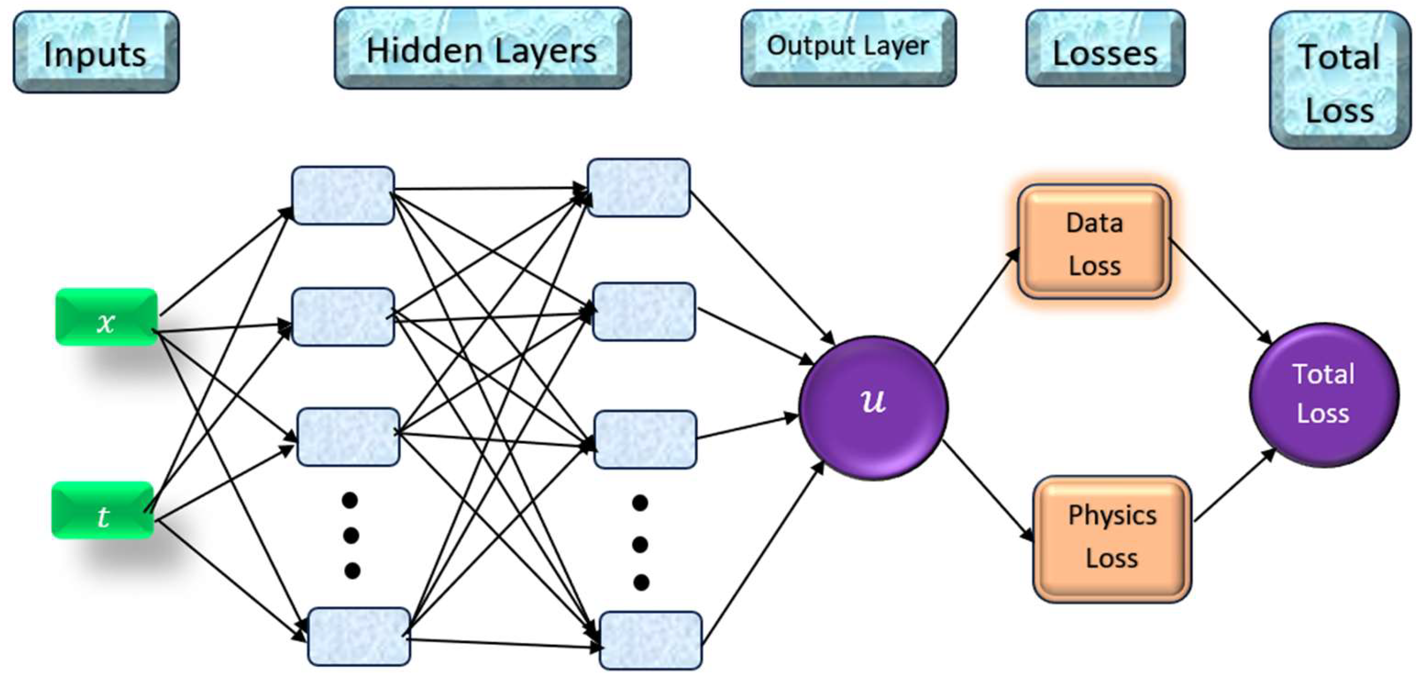
Figure 2.
Flowchart for solving the Fractional Fokker–Planck Levy equation via the FDM-APINN.
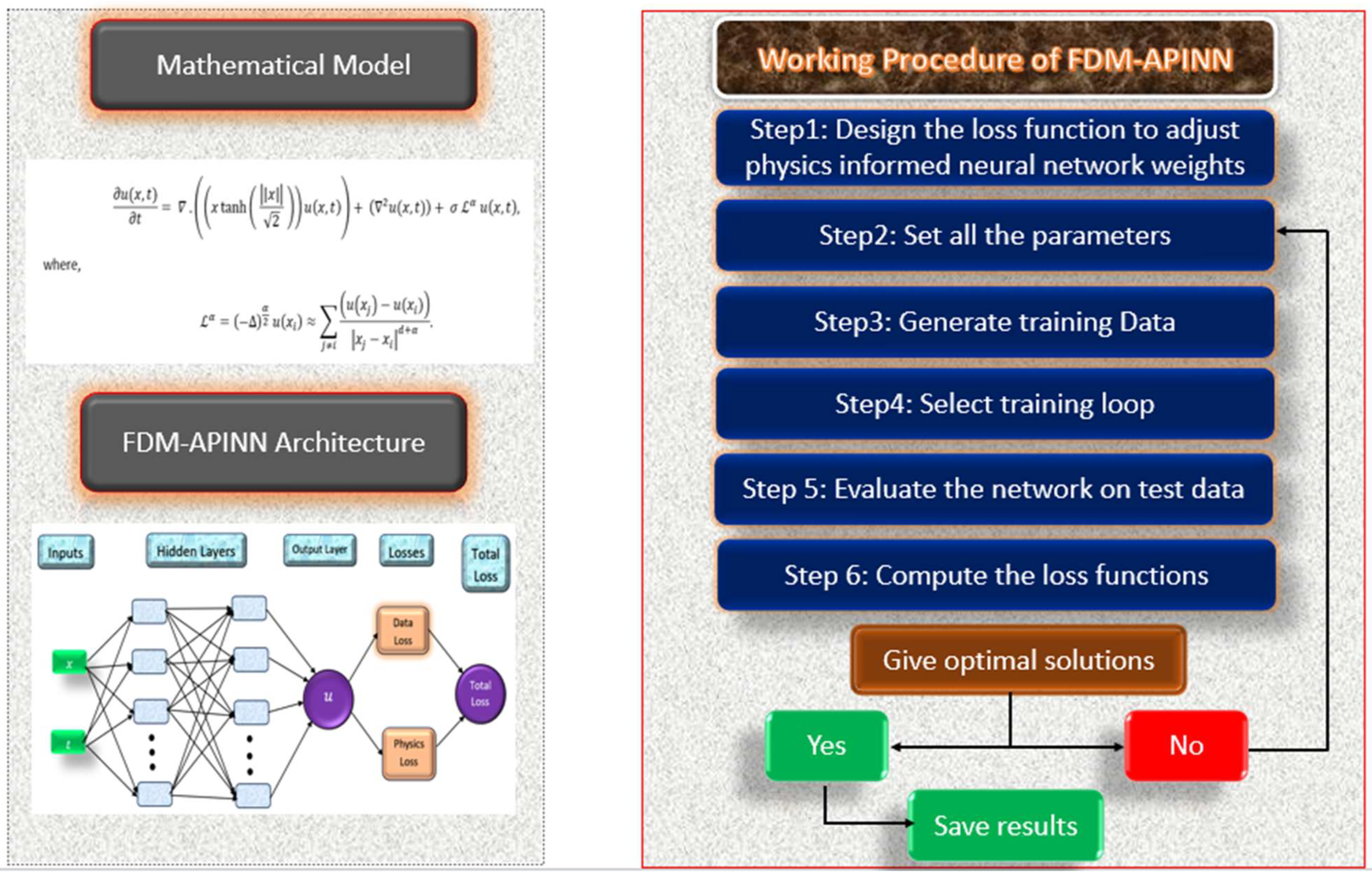
Figure 3.
Solution graphs of the Fractional Fokker Planck Levy equation.
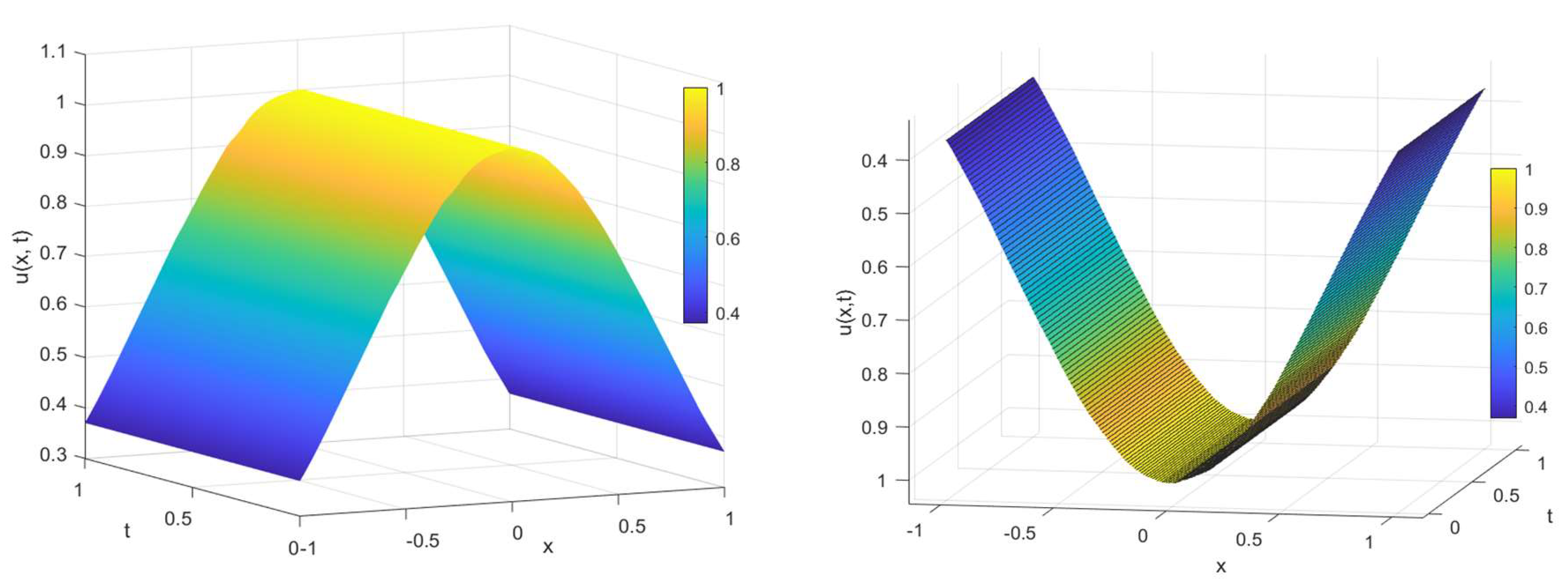
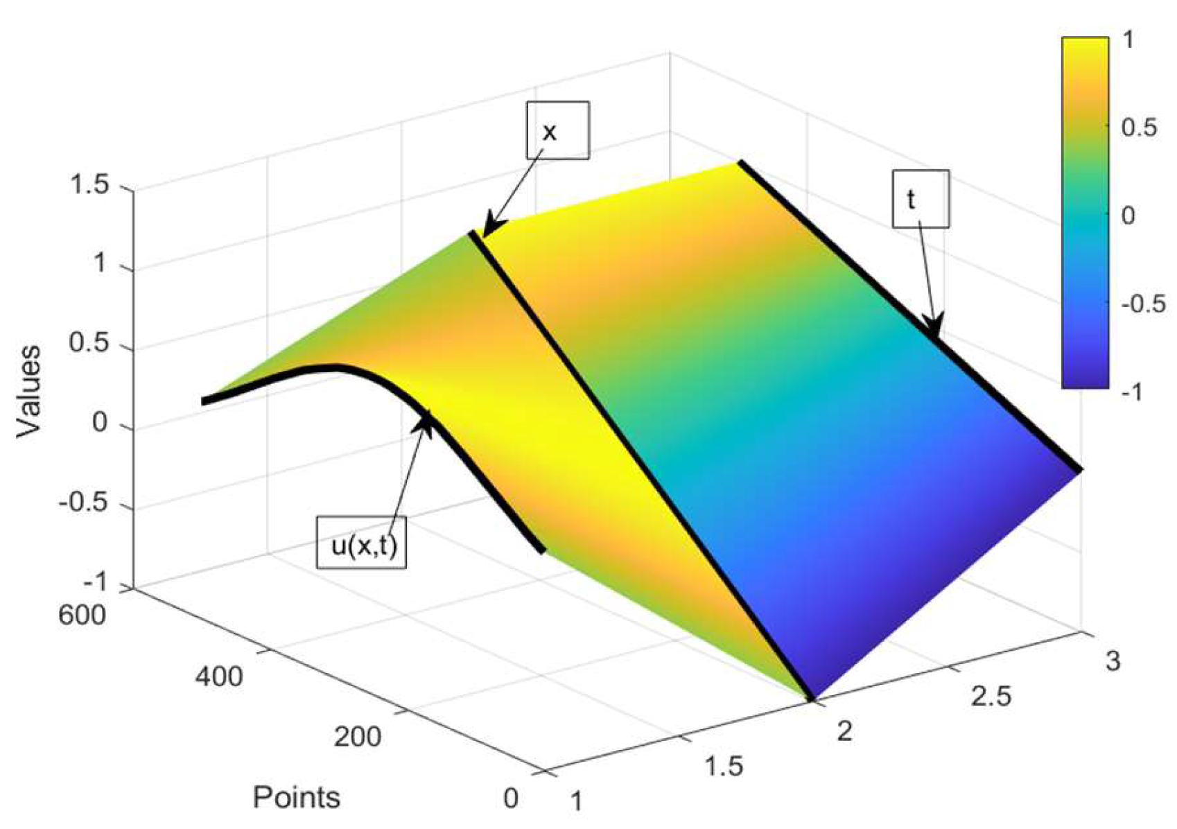
Figure 4.
Graphs of the loss and residual error values for the point distributions of the domains of and after and iterations.
Figure 4.
Graphs of the loss and residual error values for the point distributions of the domains of and after and iterations.
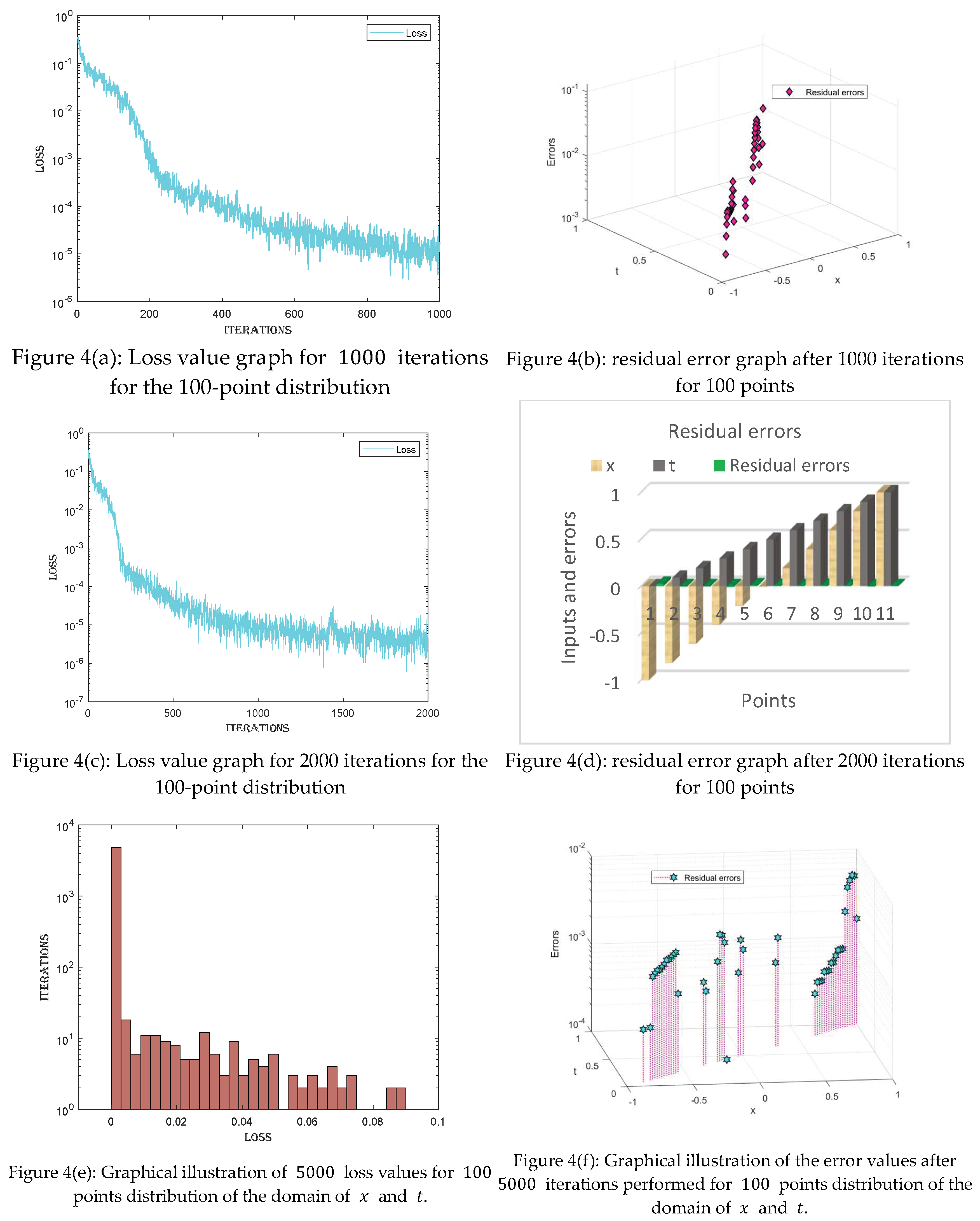
Figure 5.
Graphical illustration of the loss and residual error values after performing and iterations, respectively, for the -point distributions of the domains of and .
Figure 5.
Graphical illustration of the loss and residual error values after performing and iterations, respectively, for the -point distributions of the domains of and .
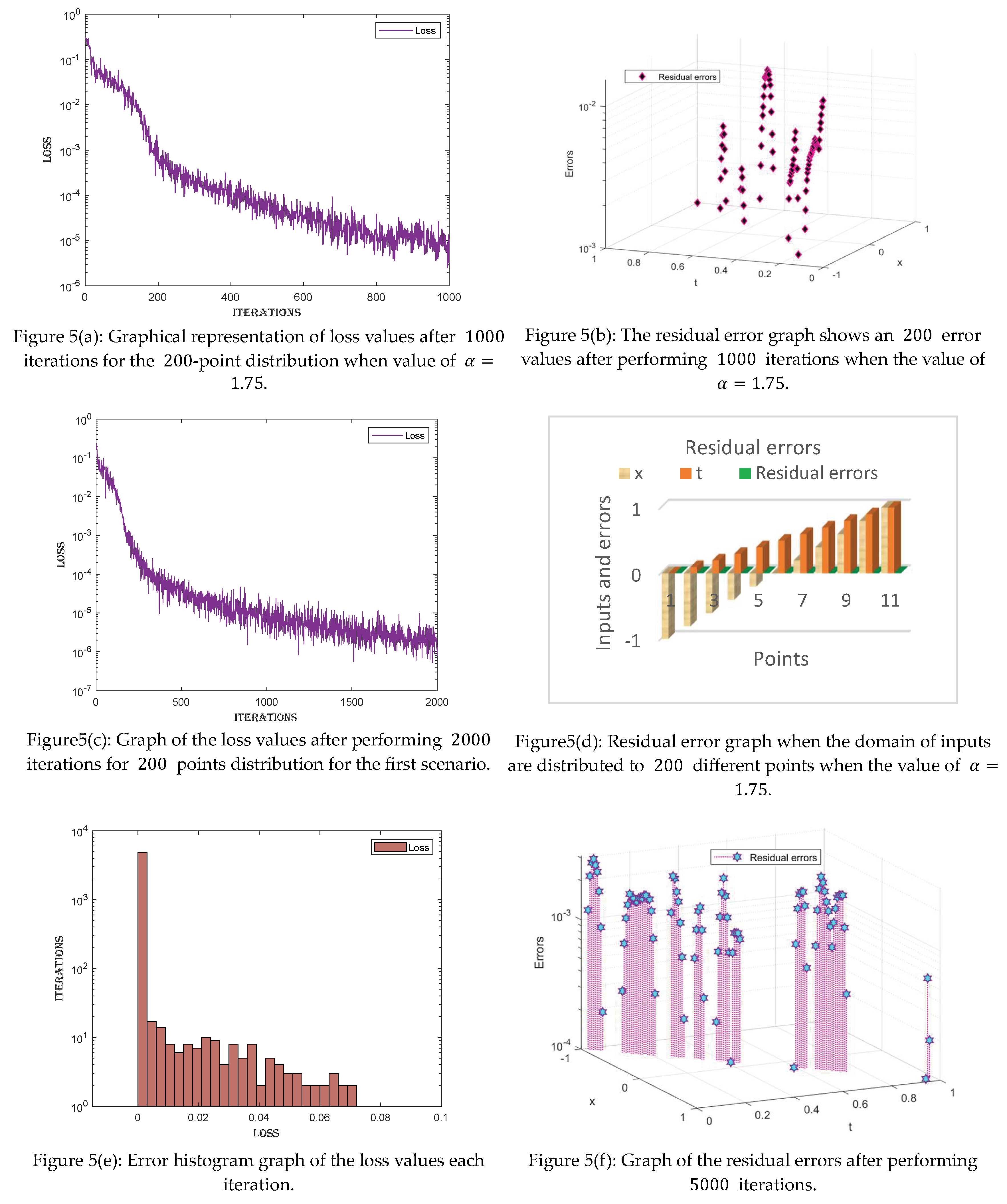
Figure 6.
Graphical illustration of all the loss and residual error values for . distribution of the domain when the value of the fractional order parameter
Figure 6.
Graphical illustration of all the loss and residual error values for . distribution of the domain when the value of the fractional order parameter
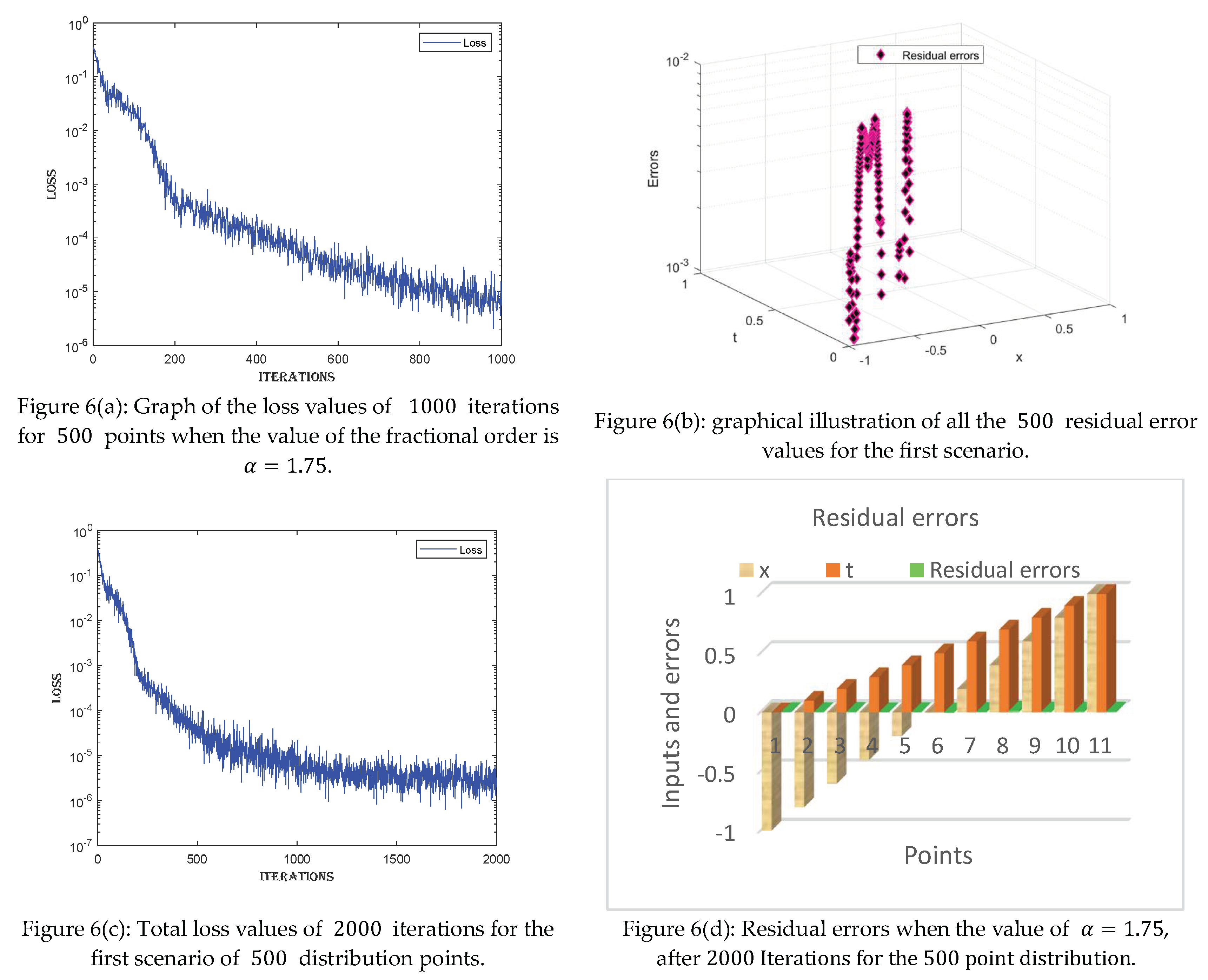
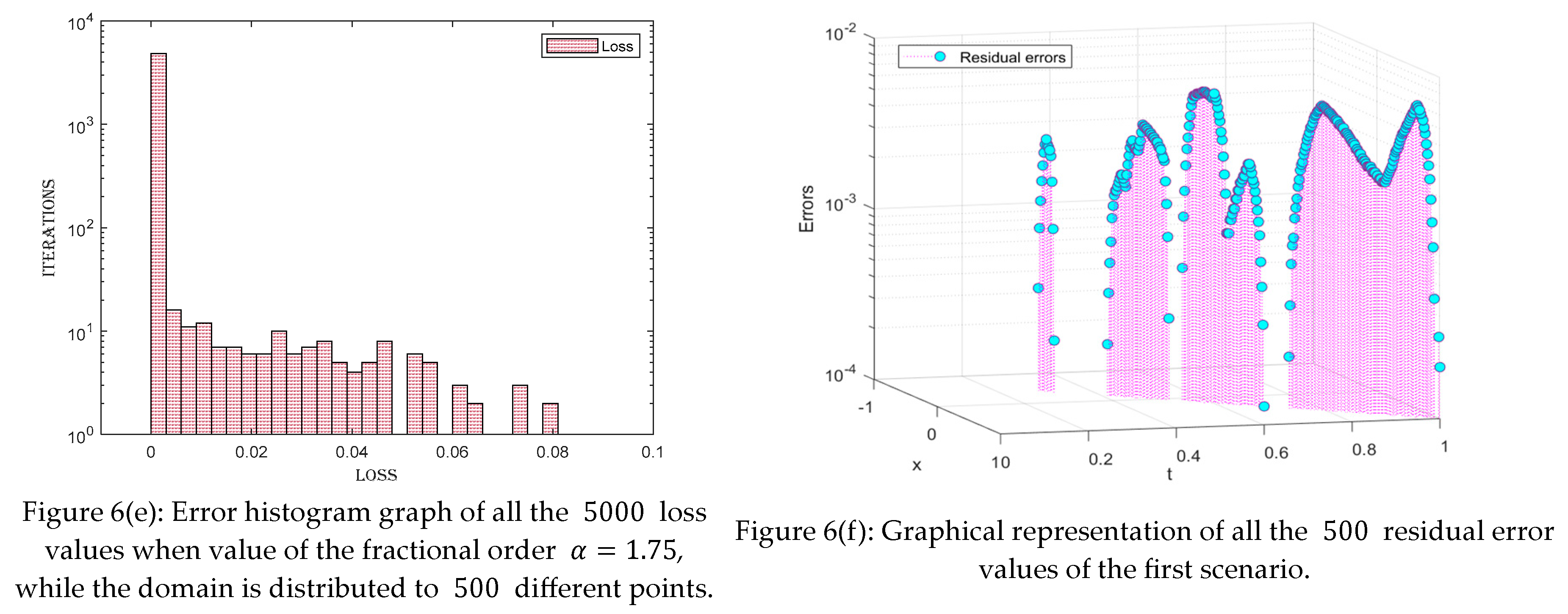
Figure 7.
Solution graphs of the FFPL equation via the FDM-APINN.
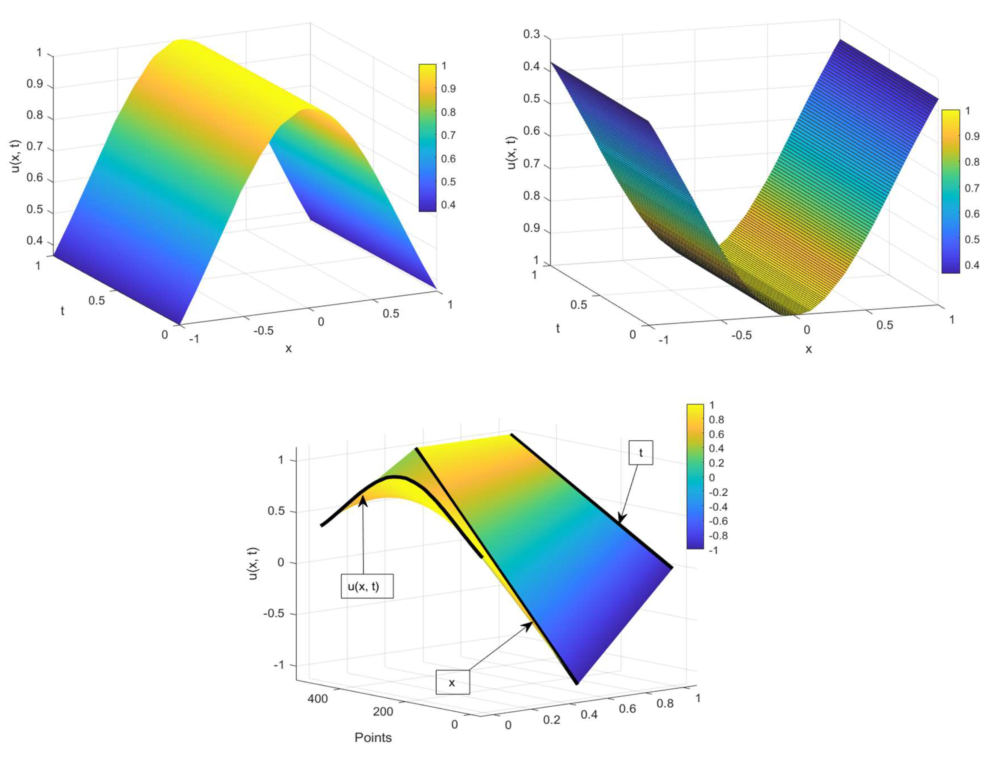
Figure 8.
Graphs of the loss and residual error values for the 100-point distribution of the domains of and after and iterations when the value of the fractional order is .
Figure 8.
Graphs of the loss and residual error values for the 100-point distribution of the domains of and after and iterations when the value of the fractional order is .
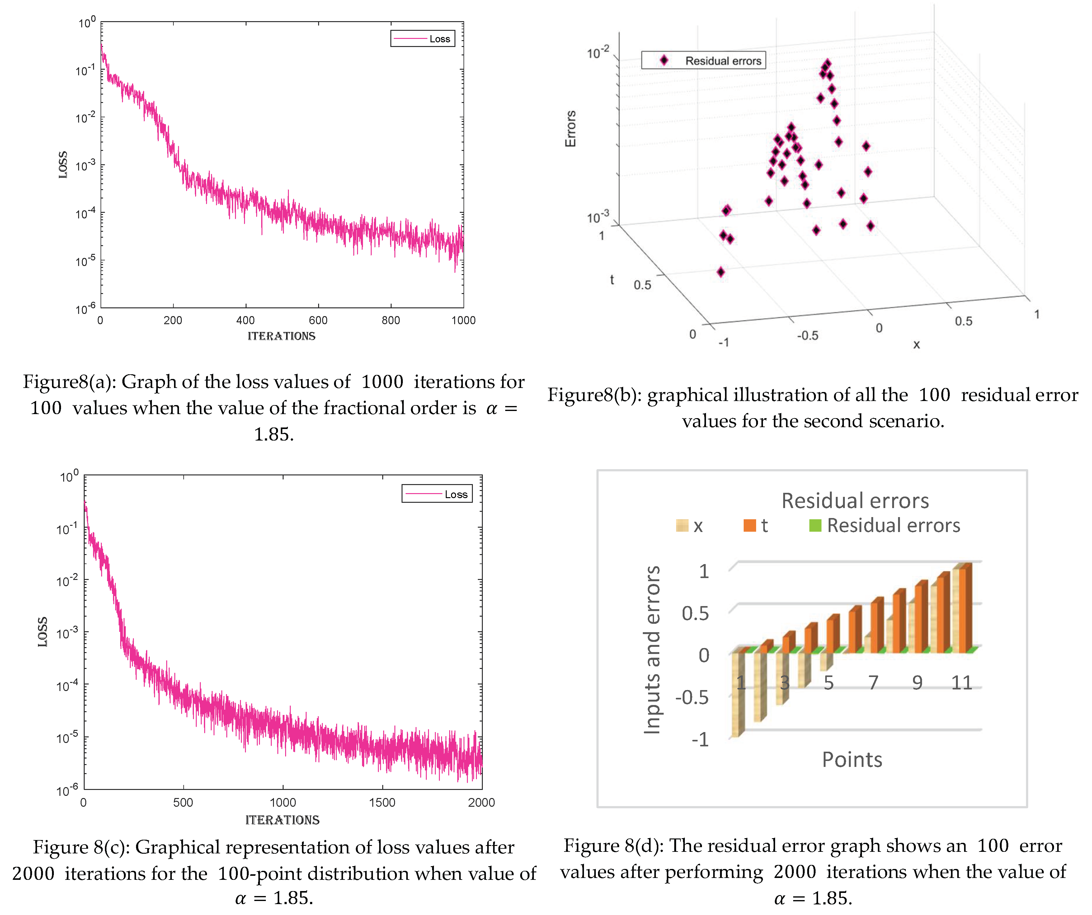
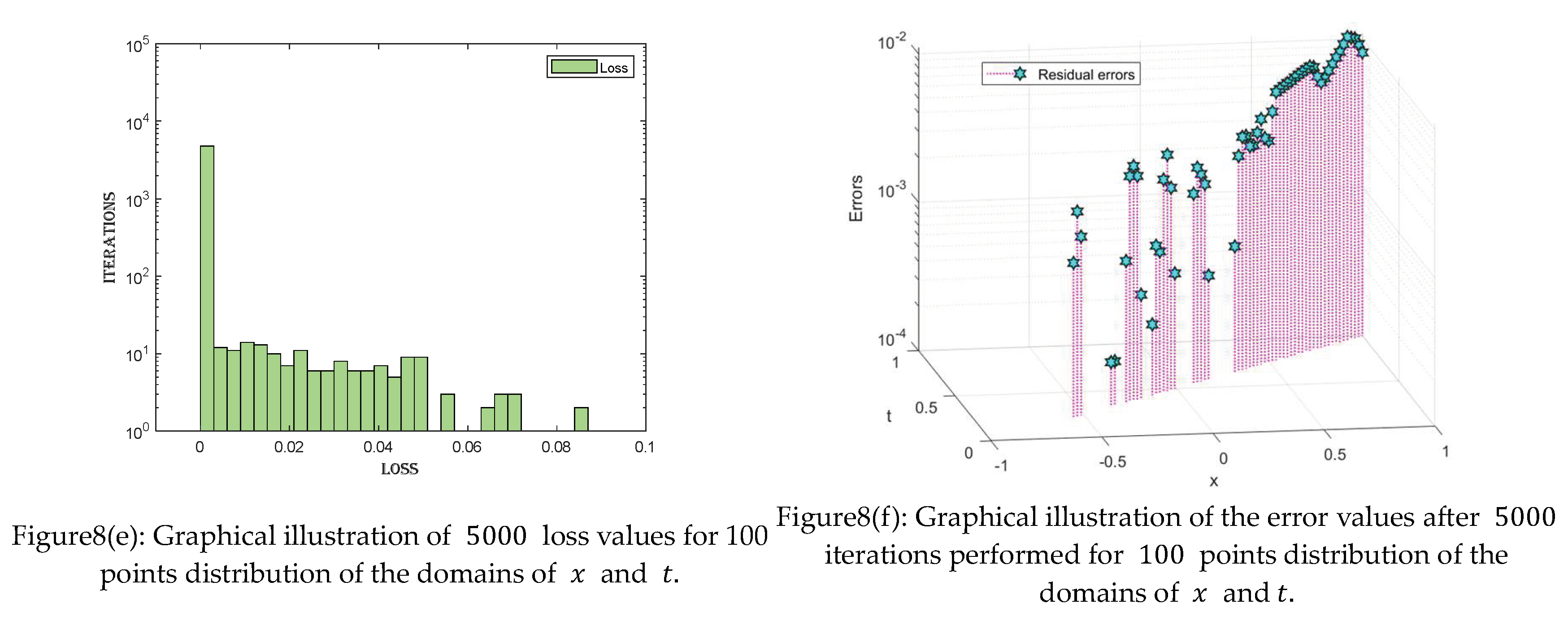
Figure 9.
Graphical illustration of all the loss and residual error values for Points distribution of the domain when the value of the fractional order parameter
Figure 9.
Graphical illustration of all the loss and residual error values for Points distribution of the domain when the value of the fractional order parameter
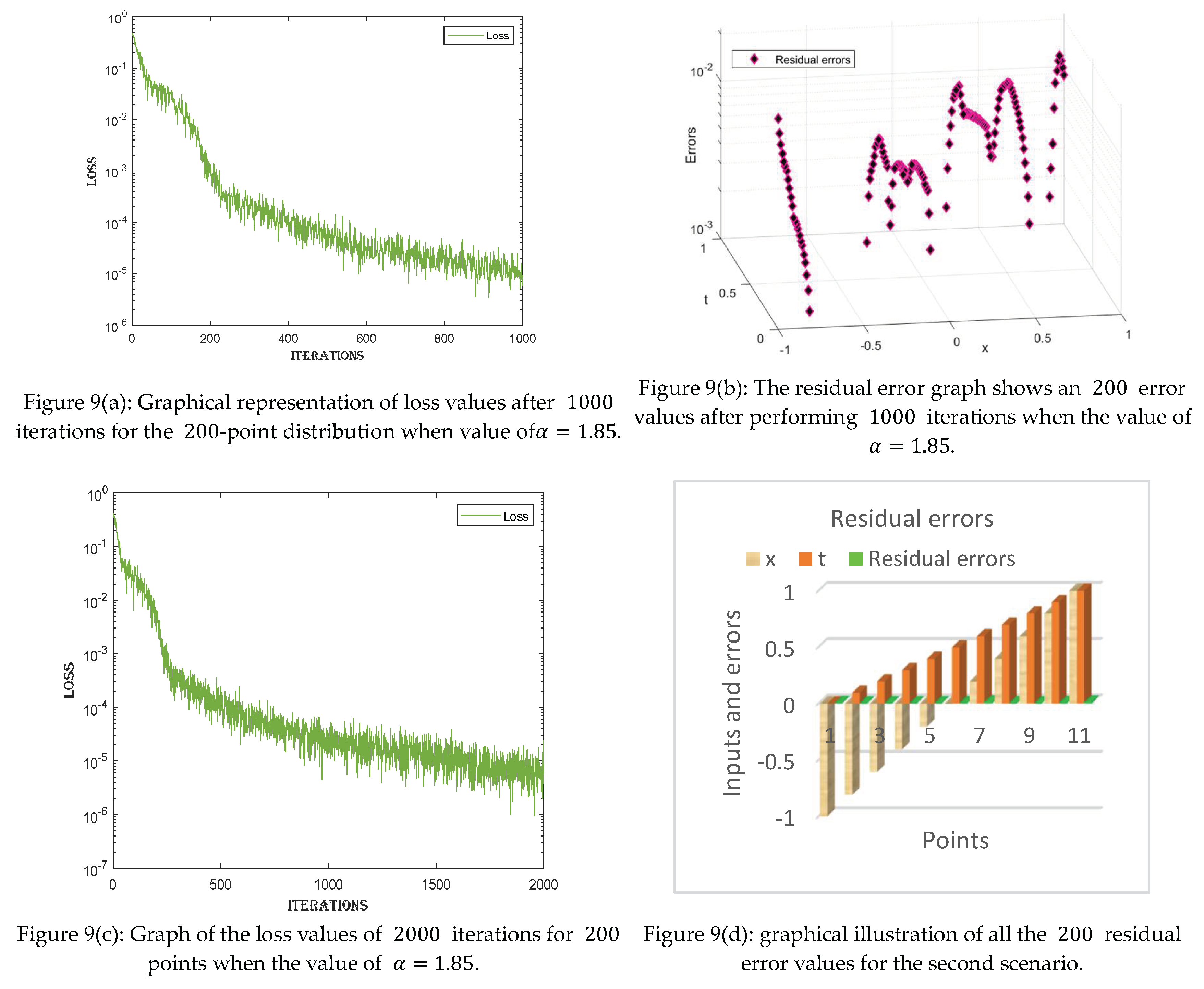
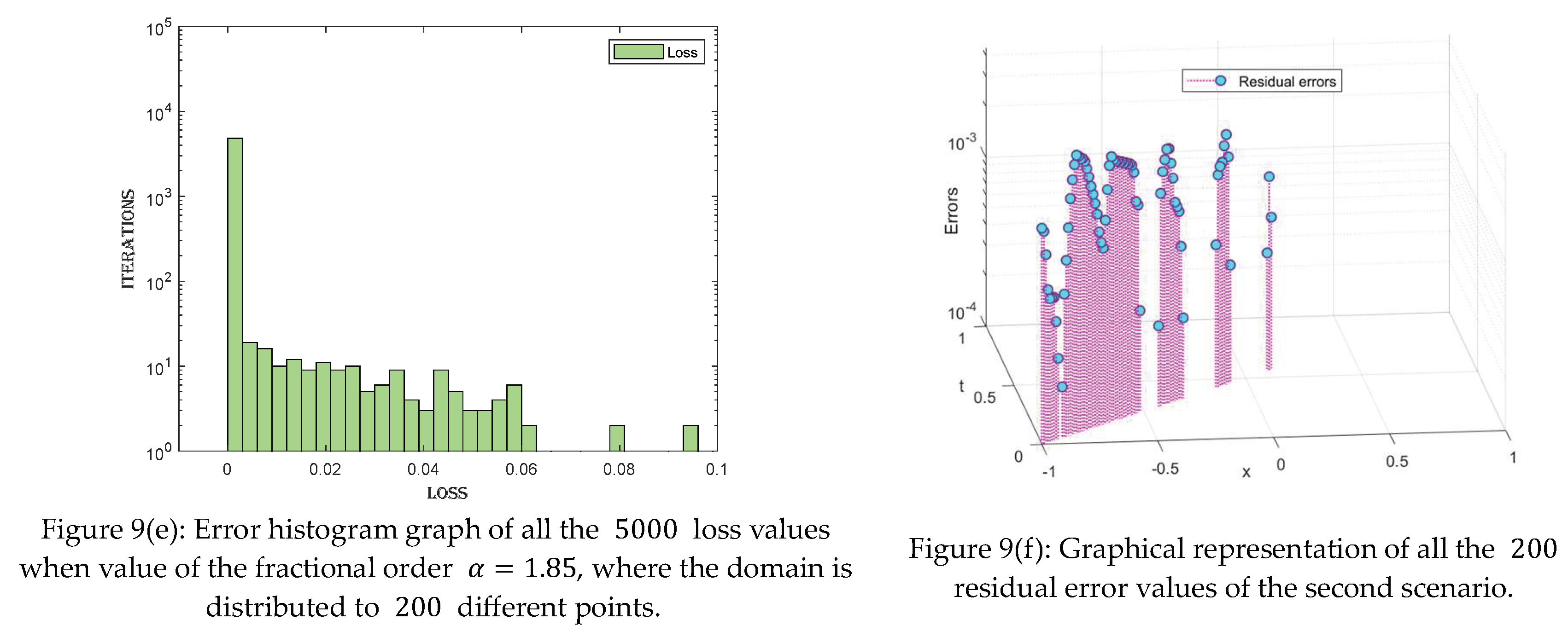
Figure 10.
Graphs showing the loss and residual error values for the 500-point distribution of the domains of and after and iterations when the value of . The graph of the loss values is shown in Figure 10(c). Figure 10(c) shows the loss values for 0 iterations of the -point distribution of the domains of and , where the value of the fractional order parameter is . The -axis of the graph represents the number of iterations, and the -axis of the graph represents the loss values. Figure 10(c) shows that as the number of iterations increases, the loss value decreases and approaches zero. This indicates that the proposed technique converges to the optimal solutions. At the start of the iterations, the loss value is not close to zero, but after iterations, the loss value approaches zero. As we approach the iterations, the loss value approaches . This means that as we approach the iteration, the solutions approach their best optimal values. Figure 10(d) shows the graph of the error values. Figure 10(d) shows the errors obtained during the iterations for the point distributions of the domains of and . Figure 10(d) shows the and error values. We take points to observe the errors. Figure 10(d) shows that the errors are very close to zero, indicating the accuracy and consistency of our proposed technique.
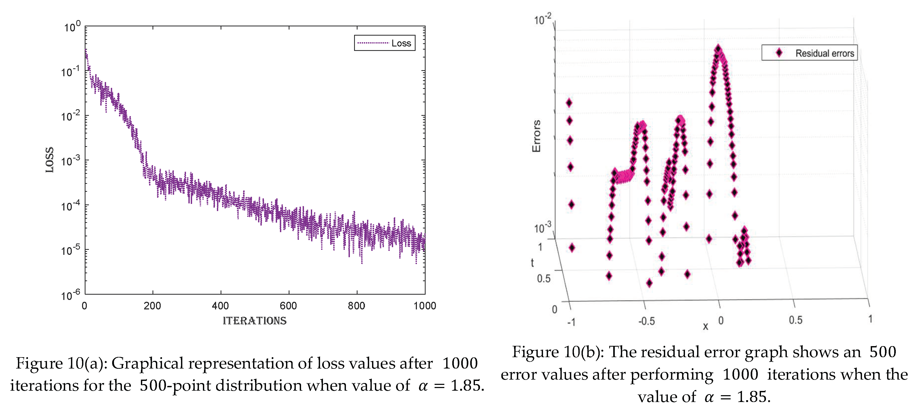
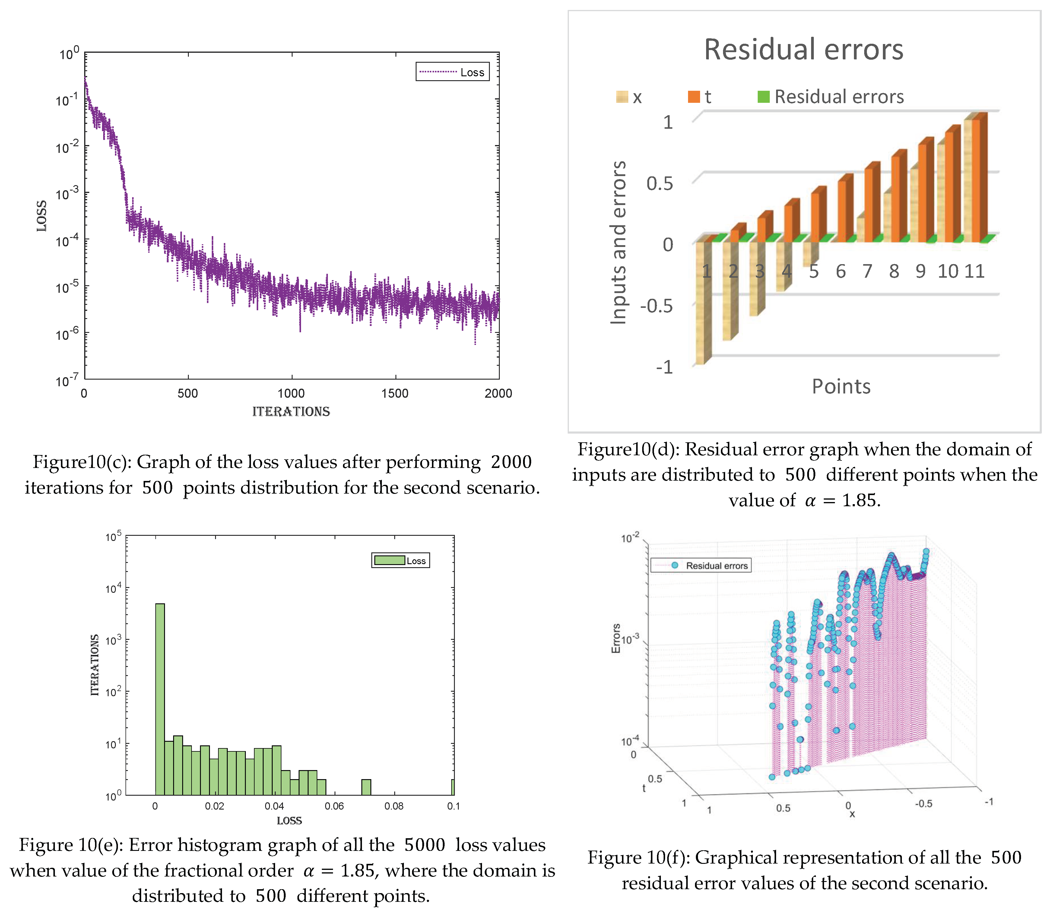

Table 1.
Table showing all the patterns of the manuscript for both scenarios.
| Scenarios | Cases | Iterations |
|---|---|---|
| 100 points | 1000 | |
| 2000 | ||
| 5000 | ||
| 200 points | 1000 | |
| 2000 | ||
| 5000 | ||
| 500 points | 1000 | |
| 2000 | ||
| 5000 | ||
| 100 points | 1000 | |
| 2000 | ||
| 5000 | ||
| 200 points | 1000 | |
| 2000 | ||
| 5000 | ||
| 500 points | 1000 | |
| 2000 | ||
| 5000 |
Table 2.
Average loss values after performing and iterations of the first scenario for and point distributions of the domains, respectively.
Table 2.
Average loss values after performing and iterations of the first scenario for and point distributions of the domains, respectively.
| Points | Iterations | Average Loss |
| 100 | 1000 | 1.7910-5 |
| 2000 | 4.69×10⁻⁶ | |
| 5000 | 1.05×10⁻⁶ | |
| 200 | 1000 | 3.17×10⁻⁶ |
| 2000 | 1.27×10⁻⁶ | |
| 5000 | 2.06×10⁻⁶ | |
| 500 | 1000 | 5.56×10⁻⁶ |
| 2000 | 2.21×10⁻⁶ | |
| 5000 | 1.12×10⁻⁶ | |
Table 3.
Residual error values of the -point distribution when the value of the fractional order parameter is .
Table 3.
Residual error values of the -point distribution when the value of the fractional order parameter is .
| Residual errors ( iterations) |
Residual errors ( iterations) |
Residual errors ( iterations) |
||
| -1.00 | 0.00 | -2.2910-2 | 2.4910-2 | -1.60×10⁻³ |
| -0.80 | 0.10 | 1.90×10⁻³ | -5.20×10⁻³ | -7.00×10⁻⁴ |
| -0.60 | 0.20 | 5.90×10⁻³ | -4.00×10⁻³ | 2.20×10⁻³ |
| -0.40 | 0.30 | 2.80×10⁻³ | -8.80×10⁻³ | -8.00×10⁻⁴ |
| -0.20 | 0.40 | -9.50×10⁻³ | 8.60×10⁻³ | 1.40×10⁻³ |
| 0.00 | 0.50 | -1.00×10⁻³ | 4.00×10⁻³ | 2.10×10⁻³ |
| 0.20 | 0.60 | -1.00×10⁻⁴ | 3.20×10⁻³ | -1.70×10⁻³ |
| 0.40 | 0.70 | -5.20×10⁻³ | 6.00×10⁻³ | -2.20×10⁻³ |
| 0.60 | 0.80 | 7.70×10⁻³ | 1.90×10⁻³ | -1.20×10⁻³ |
| 0.80 | 0.90 | 3.60×10⁻³ | -4.00×10⁻³ | 6.00×10⁻⁴ |
| 1.00 | 1.00 | 9.90×10⁻³ | 5.00×10⁻⁴ | 1.60×10⁻³ |
Table 4.
Tabular illustration of the error values of points distribution when .
| Residual error ( iterations) |
Residual error ( iterations) |
Residual error (5000 iterations) |
||
| -1.00 | 0.00 | 1.51-2 | 1.70×10⁻³ | -3.40×10⁻³ |
| -0.80 | 0.10 | 5.70×10⁻³ | 3.50×10⁻³ | -1.10×10⁻³ |
| -0.60 | 0.20 | 1.00×10⁻³ | -8.00×10⁻⁴ | 1.30×10⁻³ |
| -0.40 | 0.30 | -4.50×10⁻³ | 4.00×10⁻⁴ | -4.00×10⁻⁴ |
| -0.20 | 0.40 | 3.30×10⁻³ | 2.40×10⁻³ | 2.60×10⁻³ |
| 0.00 | 0.50 | 3.10×10⁻³ | -9.00×10⁻⁴ | -1.90×10⁻³ |
| 0.20 | 0.60 | -1.60×10⁻³ | -1.10×10⁻³ | 9.00×10⁻⁴ |
| 0.40 | 0.70 | -7.00×10⁻³ | -1.50×10⁻³ | 9.00×10⁻⁴ |
| 0.60 | 0.80 | 3.70×10⁻³ | -2.10×10⁻³ | -3.00×10⁻³ |
| 0.80 | 0.90 | -8.30×10⁻³ | 0.00 | -1.80×10⁻³ |
| 1.00 | 1.00 | 1.00×10⁻³ | 4.60×10⁻³ | -2.30×10⁻³ |
Table 5.
Residual error values for the proposed technique and the reference solutions of the points distribution when
Table 5.
Residual error values for the proposed technique and the reference solutions of the points distribution when
| .. | Residual error (1000 iteration) |
Residual error (2000 iteration) |
Residual error (5000 iteration) |
|
| -1.00 | 0.00 | 1.30×10⁻³ | 2.80×10⁻³ | -7.00×10⁻⁴ |
| -0.80 | 0.10 | 7.10×10⁻³ | 2.40×10⁻³ | -2.20×10⁻³ |
| -0.60 | 0.20 | 7.20×10⁻³ | 3.70×10⁻³ | -3.70×10⁻³ |
| -0.40 | 0.30 | -6.00×10⁻⁴ | 1.20×10⁻³ | 2.10×10⁻³ |
| -0.20 | 0.40 | -6.40×10⁻³ | 1.80×10⁻³ | -1.70×10⁻³ |
| 0.00 | 0.50 | 2.30×10⁻³ | -5.10×10⁻³ | 3.20×10⁻³ |
| 0.20 | 0.60 | -5.10×10⁻³ | 4.10×10⁻³ | 6.20×10⁻³ |
| 0.40 | 0.70 | -5.20×10⁻³ | 1.4610-2 | -2.00×10⁻⁴ |
| 0.60 | 0.80 | -1.3310-2 | 6.00×10⁻³ | 5.80×10⁻³ |
| 0.80 | 0.90 | -9.40×10⁻³ | 6.50×10⁻³ | 2.30×10⁻³ |
| 1.00 | 1.00 | 1.00×10⁻⁴ | 6.00×10⁻³ | 2.00×10⁻⁴ |
Table 6.
Residual error values of the 100-point distribution when the value of the fractional order parameter is .
Table 6.
Residual error values of the 100-point distribution when the value of the fractional order parameter is .
| Points | Iterations | Average Loss |
| 100 | 1000 | 3.38×10⁻⁵ |
| 2000 | 2.63×10⁻⁶ | |
| 5000 | 1.90×10⁻⁶ | |
| 200 | 1000 | 9.25×10⁻⁶ |
| 2000 | 5.61×10⁻⁶ | |
| 5000 | 3.30×10⁻⁶ | |
| 500 | 1000 | 2.36×10⁻⁵ |
| 2000 | 4.27×10⁻⁶ | |
| 5000 | 4.33×10⁻⁶ | |
Table 7.
Residual error values for the proposed technique and the reference solutions of the points distribution when
Table 7.
Residual error values for the proposed technique and the reference solutions of the points distribution when
| .. | Residual error (1000 iteration) |
Residual error (2000 iteration) |
Residual error (5000 iteration) |
|
| -1.00 | 0.00 | -5.00×10⁻⁴ | 3.10×10⁻³ | -1.3610-2 |
| -0.80 | 0.10 | 2.80×10⁻³ | 1.60×10⁻³ | -6.00×10⁻³ |
| -0.60 | 0.20 | -1.80×10⁻³ | -2.70×10⁻³ | -2.40×10⁻³ |
| -0.40 | 0.30 | 6.60×10⁻³ | -1.1810-2 | -3.20×10⁻³ |
| -0.20 | 0.40 | 5.80×10⁻³ | 9.00×10⁻⁴ | 3.20×10⁻³ |
| 0.00 | 0.50 | 9.80×10⁻³ | -1.80×10⁻³ | 6.00×10⁻⁴ |
| 0.20 | 0.60 | 1.40×10⁻³ | -2.30×10⁻³ | -1.90×10⁻³ |
| 0.40 | 0.70 | 3.50×10⁻³ | 1.30×10⁻³ | 3.10×10⁻³ |
| 0.60 | 0.80 | -6.00×10⁻³ | 1.40×10⁻³ | 7.00×10⁻³ |
| 0.80 | 0.90 | -7.60×10⁻³ | -6.00×10⁻⁴ | 6.40×10⁻³ |
| 1.00 | 1.00 | 5.00×10⁻⁴ | -3.60×10⁻³ | 8.10×10⁻³ |
Table 8.
Residual error values between the proposed technique and the reference solutions of the 200-point distribution when
Table 8.
Residual error values between the proposed technique and the reference solutions of the 200-point distribution when
| . | Residual error (1000 iteration) |
Residual error (2000 iteration) |
Residual error (5000 iteration) |
|
| -1.00 | 0.00 | 2.17×10⁻² | 3.10×10⁻³ | 1.90×10⁻³ |
| -0.80 | 0.10 | 2.30×10⁻³ | -6.00×10⁻⁴ | 4.10×10⁻³ |
| -0.60 | 0.20 | -3.10×10⁻³ | 3.00×10⁻⁴ | 3.30×10⁻³ |
| -0.40 | 0.30 | -4.00×10⁻³ | 2.00×10⁻⁴ | 2.40×10⁻³ |
| -0.20 | 0.40 | 3.30×10⁻³ | 9.00×10⁻⁴ | -4.10×10⁻³ |
| 0.00 | 0.50 | 4.60×10⁻³ | 1.90×10⁻³ | -2.50×10⁻³ |
| 0.20 | 0.60 | 6.00×10⁻³ | 9.60×10⁻³ | -3.20×10⁻³ |
| 0.40 | 0.70 | 7.30×10⁻³ | 1.60×10⁻³ | -2.30×10⁻³ |
| 0.60 | 0.80 | 1.06×10⁻² | -7.00×10⁻⁴ | -4.20×10⁻³ |
| 0.80 | 0.90 | -4.00×10⁻⁴ | 3.30×10⁻³ | -6.50×10⁻³ |
| 1.00 | 1.00 | 8.80×10⁻³ | 7.90×10⁻³ | -1.21×10⁻² |
Table 9.
Residual error values of the -point distribution when the value of the fractional order parameter is .
Table 9.
Residual error values of the -point distribution when the value of the fractional order parameter is .
| Residual error (1000 iteration) |
Residual error (2000 iteration) |
Residual error (5000 iteration) |
||
| -1.00 | 0.00 | 9.00×10⁻³ | 8.50×10⁻³ | 7.00×10⁻³ |
| -0.80 | 0.10 | -2.10×10⁻³ | 1.29×10⁻² | 5.30×10⁻³ |
| -0.60 | 0.20 | 3.40×10⁻³ | 9.50×10⁻³ | 3.30×10⁻³ |
| -0.40 | 0.30 | -2.60×10⁻³ | 2.00×10⁻³ | 4.80×10⁻³ |
| -0.20 | 0.40 | 5.30×10⁻³ | 5.00×10⁻³ | 5.00×10⁻⁴ |
| 0.00 | 0.50 | 5.10×10⁻³ | -6.00×10⁻⁴ | 1.80×10⁻³ |
| 0.20 | 0.60 | 1.20×10⁻³ | 4.20×10⁻³ | 2.50×10⁻³ |
| 0.40 | 0.70 | -3.60×10⁻³ | 1.10×10⁻³ | -4.20×10⁻³ |
| 0.60 | 0.80 | -5.70×10⁻³ | -7.70×10⁻³ | -2.50×10⁻³ |
| 0.80 | 0.90 | -2.80×10⁻³ | -4.50×10⁻³ | -5.80×10⁻³ |
| 1.00 | 1.00 | -1.95×10⁻² | -7.90×10⁻³ | -5.30×10⁻³ |
Disclaimer/Publisher’s Note: The statements, opinions and data contained in all publications are solely those of the individual author(s) and contributor(s) and not of MDPI and/or the editor(s). MDPI and/or the editor(s) disclaim responsibility for any injury to people or property resulting from any ideas, methods, instructions or products referred to in the content. |
© 2024 by the authors. Licensee MDPI, Basel, Switzerland. This article is an open access article distributed under the terms and conditions of the Creative Commons Attribution (CC BY) license (http://creativecommons.org/licenses/by/4.0/).
Copyright: This open access article is published under a Creative Commons CC BY 4.0 license, which permit the free download, distribution, and reuse, provided that the author and preprint are cited in any reuse.


