
Submitted:
03 November 2023
Posted:
03 November 2023
You are already at the latest version
Abstract
This study develops a new definition of fractional derivative that mixes the definitions of fractional derivatives with singular and non-singular kernels. Such developed definition encompasses many types of fractional derivatives, such as the Riemann-Liouville and Caputo fractional derivatives for singular kernel type as well as the Caputo-Fabrizio, the Atangana-Baleanu and the generalized Hattaf fractional derivatives for non-singular kernel type. The associate fractional integral of the new mixed fractional derivative is rigorously introduced. Furthermore, newly numerical scheme is developed to approximate the solutions of a class of fractional differential equations (FDEs) involving the mixed fractional derivative. Finally, an application to computational biology is presented.
Keywords:
Fractional operators
; singular and non-singular kernels
; Laplace transform
; numerical method
1. Introduction
In recent years, fractional mathematical modeling involving nonlocal fractional derivatives plays a robust tool and constitutes a new resource to capture the dynamics of complex systems having memory effects or hereditary characteristics. Such systems arising from various fields including physics, fluid mechanics, material science, signal processing, engineering, chemistry, biology, medicine, finance, social sciences, economics and ecology.
In the literature, there are two main types of nonlocal fractional derivatives. The first named the fractional derivatives with singular kernels like Riemann-Liouville fractional derivative [1,2] and Caputo fractional derivative which was introduced by Caputo in 1967 [3] to find the analytic expression for a linear dissipative mechanism whose quality factor (Q) is almost frequency independent over large frequency ranges. The second ones have non-singular kernels such as the Caputo-Fabrizio (CF) derivative [4] introduced by Caputo and Fabrizio in 2015 to avoid the singularity existing in [3]. In 2016, Atangana and Baleanu [5] proposed a fractional derivative to model the flow of heat transfer through a material with different scale or heterogeneous. In 2020, Al-Refai [6] presented a weighted fractional derivative based on Atangana-Baleanu (AB) fractional derivative [5]. By means of the Laplace transform, he solved an associated linear fractional differential equation.
Recently, a new generalized Hattaf fractional (GHF) derivative with non-singular kernel has been introduced in [7] to cover the CF [4], the AB [5] and the weighted AB [6] fractional derivatives. A new class of fractal-fractional derivatives was derived from the GHF derivative and the new generalized fractal derivative [8] that covers the Hausdorff fractal derivative [9] used to model the anomalous diffusion process. Furthermore, the new GHF derivative was used by many researchers to describe the dynamics of various phenomena arising from several areas of science and engineering [10,11,12,13,14].
The first aim of the present paper is to introduce a new definition of nonlocal fractional derivative that includes and generalizes numerous fractional derivatives with singular and non-singular kernels such as Riemann-Liouville [1,2], Caputo [3], CF [4], AB [5] and the weighted AB [6] fractional derivatives. The new introduced definition also includes the GHF derivative [7], the power fractional derivative [15], as well as the new fractional derivative with Mittag-Leffler kernel of two parameters intoduced in [16] and applied to thermal science.
On the other hand, most fractional differential equations (FDEs) involving nonlocal fractional derivatives are complex and cannot solved analytically. For this reason, various numerical methods have been proposed to approximate the solutions of such FDEs. For instance, a numerical method that recovers the classical Euler’s scheme for ordinary differential equations (ODEs) was introduced in [17] to approximate the solutions of FDEs with GHF derivative. Another numerical method for GHF derivative was developed in [18] to solve numerically nonlinear biological systems of FDEs arising from virology.
The second aim of this paper is to develop a numerical method to approximate the solutions of FDEs with the new mixed fractional derivative mentioned in the first objective. The developed numerical method includes the three recent numerical schemes presented in [18,19,20] and it is based on Lagrange polynomial interpolation.
The remainder of the present paper is organized as follows. Section 2 defines the new mixed fractional derivative in both Caputo and Riemann-Liouville senses and presents the particular cases of such mixed fractional derivative available in the previous studies. Section 3 deals with Laplace transform of the new mixed fractional derivative. Section 4 gives the fractional integral associated to the new mixed fractional derivative and its special cases. Section 5 establishes new important formulas and properties for the new differential and integral operators. Furthermore, Section 6 is devoted to the new developed numerical method. Finally, Section 8 ends the paper with an application to computational biology.
2. The new mixed fractional derivative
This section defines the new mixed fractional derivative in the sense of Caputo and Riemann-Liouville.
Definition 2.1.
Let , and . The mixed fractional derivative of the function of order p in Caputo sense with respect to the weight function is given as follows:
where , , on [a,b], is a normalization function such that , and is the Wiman function [21] called also Mittag-Leffler function with two parameters r and q.
Definition 2.1 includes several existing fractional derivatives with singular and non-singular kernels. For instance,
- When and , we get the Caputo fractional derivative [3] with singular kernel given by
- When and , we obtain the CF fractional derivative [4] with non-singular given bywhere .
- When , and , we get the AB fractional derivative [5] given by
- When and , we find the weighted AB fractional derivative [6] given by
- When , we obtain the GHF derivative [7] given by
- When , and (with ), we get the power fractional derivative [15] given by
- When , and , we obtain the fractional derivative introduced in [16] given by
Now, we define the new mixed fractional derivative in Riemann-Liouville sense.
Definition 2.2.
Let , and . The mixed fractional derivative of the function of order p in Riemann-Liouville sense with respect to the weight function is given as follows:
Obviously, when and , we obtain the Riemann-Liouville fractional derivative [1,2] with singular kernel. In addition, we have the following result.
Theorem 2.3.
Let be an analytic function. Then
Proof.
We have is an analytic function. Then and
This ends the proof. □
3. Laplace transform of the new mixed fractional derivative
In this section, we first need the following result.
Lemma 3.1.
The Laplace transform of is given by
If , then
Proof.
According to the definition of the Wiman function, we get
In particular, if , then
This completes the proof. □
By a simple application of Lemma 3.1, we obtain the following theorem.
Theorem 3.2.
- (i)
- The Laplace transform of is given byIn particular, we have
- (ii)
- The Laplace transform of is given byIn particular, we have
Remark 3.3.
Lemma 3.1 and Theorem 3.2 extend the results presented in [7] for the new GHF derivative, it suffices to take .
4. The associate fractional integral
In this section, we define the fractional integral associated to the new mixed fractional derivative. First, we consider the following fractional differential equation:
Lemma 4.1.
Eq. (10) has a unique solution given by
where is the standard weighted Riemann-Liouville fractional integral of order α given by
Proof.
-
When , we haveBy taking the inverse Laplace, we getHence,
-
When , we haveBy passage to the inverse Laplace, we obtainwhich leads to
This completes the proof. □
Definition 4.2.
If , then the fractional integral associated to the new mixed fractional derivative is defined as follows
Remark 4.3.
The associate integral defined above includes a variety of fractional integral operators. For instance,
- (i)
- (ii)
- (iii)
- If , then (15) reduced to the standard weighted Riemann-Liouville fractional integral of order r and to ordinary integral when and .
5. Fondamental properties of the new differential and integral operators
In this section, we establish new important formulas and properties for the new differential and integral operators.
For simplicity, we denote by and by .
Lemma 5.1.
The mixed fractional derivative can be expressed as follows:
Proof.
Since the Mittag-Leffler function is an entire function of t, then can be expressed as follows:
This ends the proof. □
Remark 5.2.
Lemma 5.1 extends the recent result established by Zitane and Torres in Lemma 3 of [20].
Theorem 5.3.
Let , , and . Then, we have the following property:
Proof.
When , we have
By applying Lemma 5.1, we get
For , we have
Hence, the proof is completed. □
It is obvious that when , we obtain the following first corollary of Theorem 5.3 that extends the Newton-Leibniz formula given in [22].
Corollary 5.4.
The new mixed fractional derivative and integral satisfy the Newton-Leibniz formula. In other words, we have
Clearly, for all constant function . Moreover, we have the following result.
Corollary 5.5.
Let u be a solution of the following fractional differential equation
Then the function u is a constant function.
Proof.
It follows from (18) that . This proves that u is a constant function. □
6. Numerical scheme
In this section, we first develop a numerical method to approximate the solution of the following FDE with the new mixed fractional derivative given by
subject to the given initial condition
From Theorem 5.3, Eq. (20) can be converted into the following fractional integral equation:
So, we discuss to cases. When , we have
which implies that
Let be the discretization step and , with . We have
Then
where . The function g can be approximated over by means of the Lagrange polynomial interpolation as follows:
Hence,
Since
and
we have the following numerical scheme for the case :
where
Remark 6.1.
To illustrate our numerical scheme, we consider the following FDE with the mixed fractional derivative:
Let . By applying the fractional integral to both sides of (29) and using Theorem 5.3, we obtain the exact solution of (29), which is given by
Now, we apply the developed numerical scheme for the case presented in (27) to approximate the solution of (29). For all numerical simulations, we choose the normalisation function as follows
The comparaison between the exact and approximate solutions of (29) with the corresponding absolute errors is visualized in Figure 1 for different values of , , and . Furthermore, Table 1 presents the maximum error for numerous values of .
From Figure 1, we notice that the developed numerical scheme gives a very good agreement between the exact and approximate solutions for different values of the discretization step . Also, Table 1 shows that the convergence of the numerical approximation depends on the discretization step . By comparing the exact and approximate solutions, we deduce that the new developed numerical scheme is very effective and rapidly converges to the exact solution.
7. Application to computational biology
Computational biology is a branch of biology used mathematical modeling and computational simulations in order to understand biological systems and relationships. Now, consider the following FDE system describing the evolution of cell population in human body:
where is the total cell population produced at rate and die naturally at rate d. Applying Laplace transform to (32), we get
According Theorem 3.2, we have
Then
where . Hence,
Thus,
On the other hand, we have
This leads to
When the weight function is constant, Eq. (33) becomes
Funding
This research received no external funding.
Institutional Review Board Statement
Not applicable.
Informed Consent Statement
Not applicable.
Data Availability Statement
Not applicable.
Conflicts of Interest
The author declares no conflicts of interest.
References
- A. A. Kilbas, H. M. Srivastava, J. J. Trujillo, Theory and Applications of Fractional Differential Equations, North-Holland Mathematics Studies, Elsevier, Amsterdam, 2006.
- I. Podlubny, Fractional Differential Equations, Academic Press, San Diego, 1999.
- M. Caputo, Linear models of dissipation whose Q is almost frequency independent-II, Geophysical Journal International 13 (1967) 529–539. [CrossRef]
- M. Caputo, M. Fabrizio, A new definition of fractional derivative without singular kernel, Progress Fractional Differention and Applications (2015) 73–85.
- A. Atangana, D. Baleanu, New fractional derivatives with non-local and non-singular kernel: theory and application to heat transfer model, Thermal Science 20 (2016) 763–769.
- M. Al-Refai, On weighted Atangana-Baleanu fractional operators, Advances in Difference Equations 2020 (2020) 1–11. [CrossRef]
- K. Hattaf, A new generalized definition of fractional derivative with non-singular kernel, Computation 8 (2) (2020) 1–9. [CrossRef]
- K. Hattaf, A new class of generalized fractal and fractal-fractional derivatives with non-singular kernels, Fractal Fractional 7 (5) (2023) 1–16. [CrossRef]
- W. Chen, Time-space fabric underlying anomalous diffusion, Chaos Solitons Fractals 28 (2006) 923–929. [CrossRef]
- K. Hattaf, Stability of fractional differential equations with new generalized Hattaf fractional derivative, Mathematical Problems in Engineering, 2021 (2021) 1–7. [CrossRef]
- Asma, M. Yousaf, M. Afzaal, M. H. DarAssi, M. A. Khan, M. Y. Alshahrani, M. Suliman, A mathematical model of vaccinations using new fractional order derivative, Vaccines 10 (12) (2022) 1980. [CrossRef]
- K. R. Cheneke, K. P. Rao, G. K. Edesssa, A new generalized fractional-order derivative and bifurcation analysis of cholera and human immunodeficiency co-infection dynamic transmission, International Journal of Mathematics and Mathematical Sciences 2022 (2022) 1–15. [CrossRef]
- M. R. Lemnaouar, C. Taftaf, C., Y. Louartassi, On the controllability of fractional semilinear systems via the generalized Hattaf fractional derivative, International Journal of Dynamics and Control (2023) 1–8. [CrossRef]
- Z. Hajhouji, K. Hattaf, N. Yousfi, A generalized fractional HIV-1 infection model with humoral immunity and highly active antiretroviral therapy, Journal of Mathematics and Computer Science 32 (2) (2024) 160–174. [CrossRef]
- E. M. Lotfi, H. Zine, D. F. M. Torres and N. Yousfi, The power fractional calculus: First definitions and properties with applications to power fractional differential equations, Mathematics 10 (2022) 1–10. [CrossRef]
- S. M. Chinchole, A. P. Bhadane, A new definition of fractional derivatives with Mittag-Leffler kernel of two parameters, Communications in Mathematics and Applications 13 (1) (2022) 19–26. [CrossRef]
- K. Hattaf, On the Stability and Numerical Scheme of Fractional Differential Equations with Application to Biology, Computation 10 (6) (2022) 1–12. [CrossRef]
- K. Hattaf, Z. Hajhouji, M. A. Ichou, N. Yousfi, A Numerical Method for Fractional Differential Equations with New Generalized Hattaf Fractional Derivative, Mathematical Problems in Engineering (2022) 1–9. [CrossRef]
- M. Toufik, A. Atangana, New numerical approximation of fractional derivative with non-local and non-singular kernel: Application to chaotic models, The European Physical Journal Plus (2017) 132: 444. [CrossRef]
- H. Zitane, D. F. M. Torres, A class of fractional differential equations via power non-local and non-singular kernels: Existence, uniqueness and numerical approximations, Physica D: Nonlinear Phenomena 457 (2024) 133951. [CrossRef]
- A. Wiman, Über den fundamental satz in der theorie der funktionen Ea(x), Acta Mathematica 29 (1905) 191–201.
- D. Baleanu, A. Fernandez, On some new properties of fractional derivatives with Mittag-Leffler kernel, Communications in Nonlinear Science and Numerical Simulation 59 (2018) 444–462.
- N. Yousfi, K. Hattaf, A. Tridane, Modeling the adaptive immune response in HBV infection, Journal of Mathematical Biology 63 (2011) 933–957. [CrossRef]
- S. Eikenberry, S. Hews, J. D. Nagy, Y. Kuang, The dynamics of a delay model of HBV infection with logistic hepatocyte growth, Mathematical Biosciences and Engineering 6 (2009) 283–299.
Figure 1.
The exact and numerical solutions of (29) with the corresponding absolute errors for different values of .
Figure 1.
The exact and numerical solutions of (29) with the corresponding absolute errors for different values of .
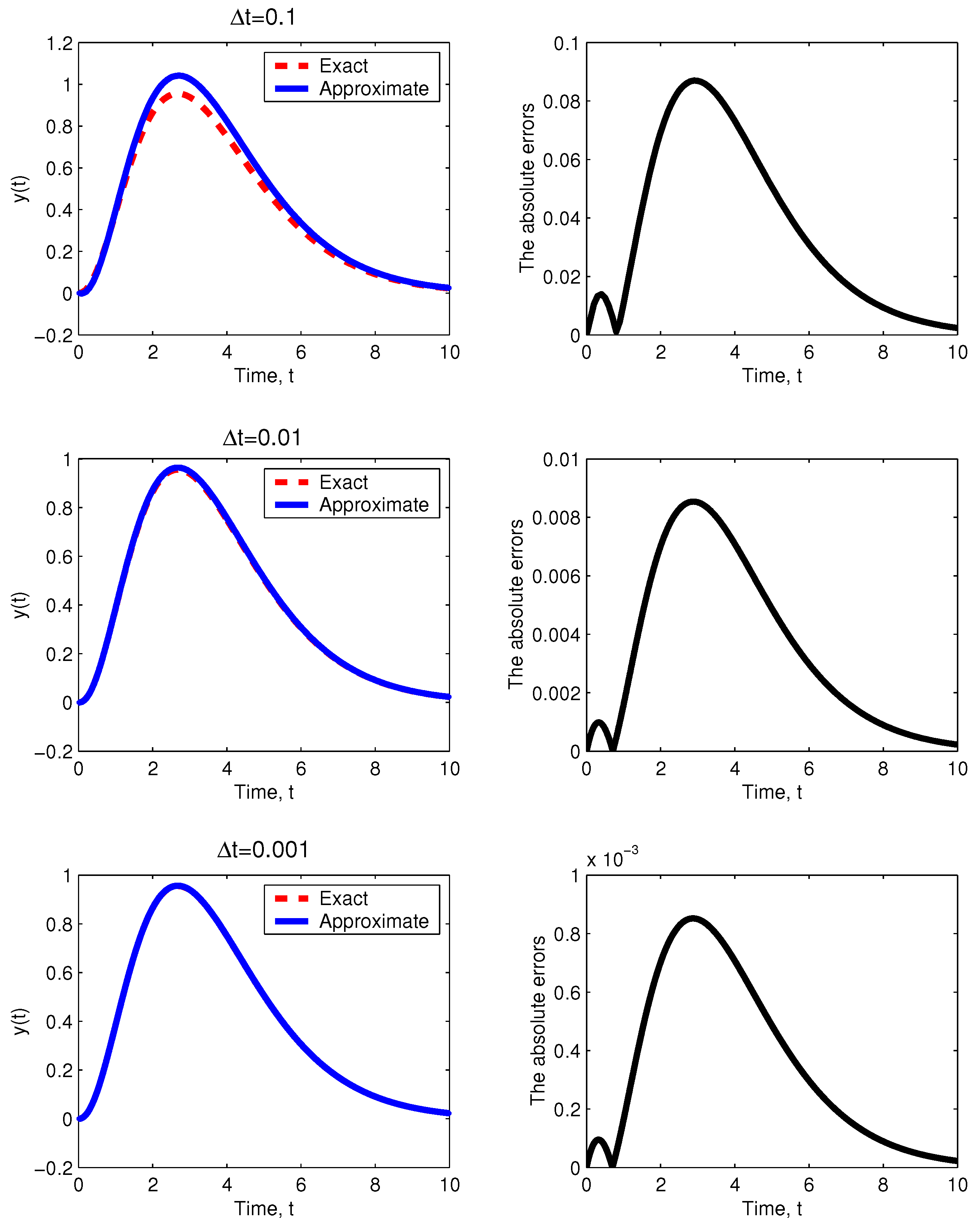
Figure 2.
Solution of (32) with two initial conditions for , and different values of p.
Figure 2.
Solution of (32) with two initial conditions for , and different values of p.
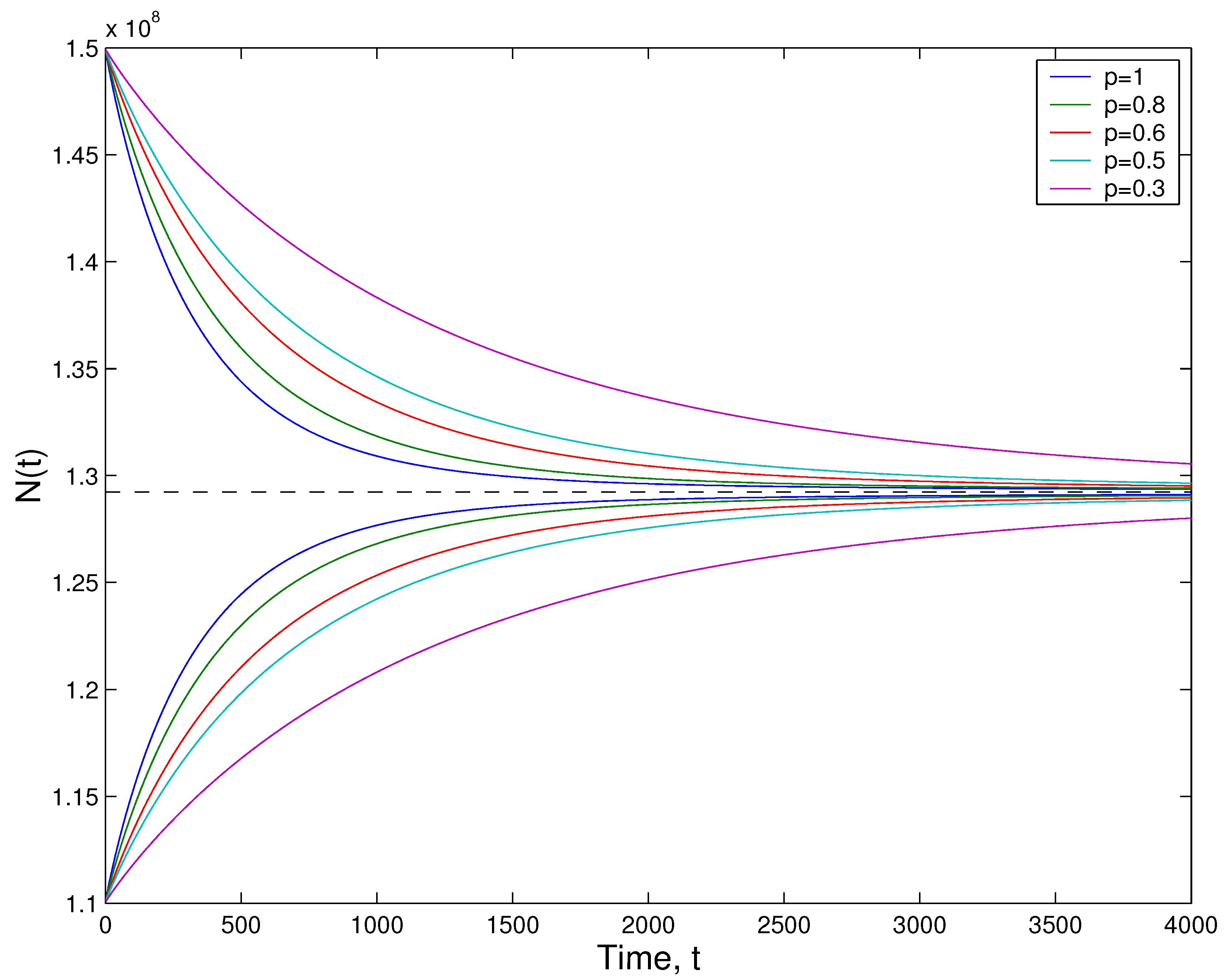
Figure 3.
Impact of the parameter on the dynamics of (32) with and .
Figure 3.
Impact of the parameter on the dynamics of (32) with and .
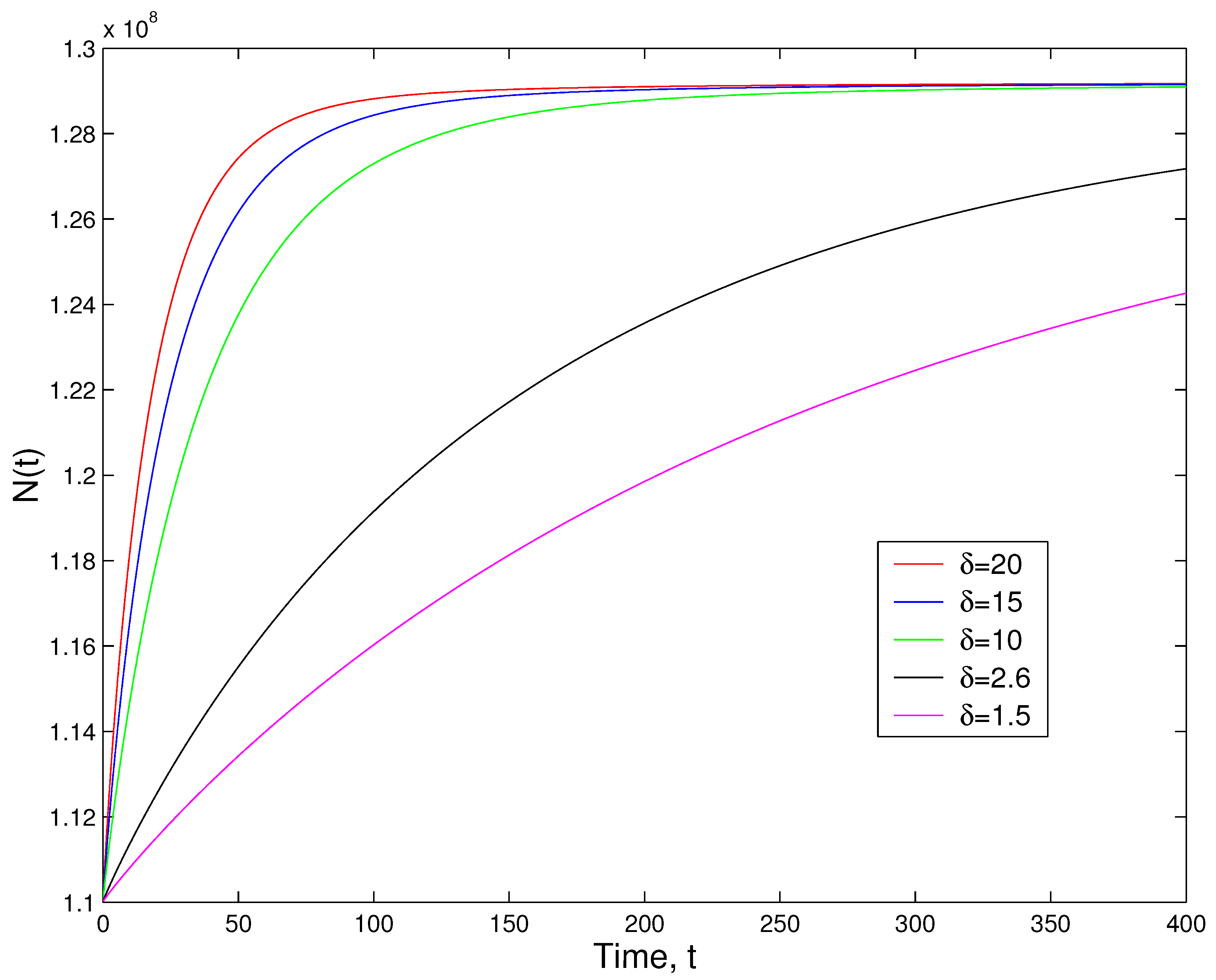

Table 1.
The maximum error corresponding to different values of with , and .
| Discretization step () | Error |
|---|---|
| 0.1 | |
| 0.01 | |
| 0.001 |
Disclaimer/Publisher’s Note: The statements, opinions and data contained in all publications are solely those of the individual author(s) and contributor(s) and not of MDPI and/or the editor(s). MDPI and/or the editor(s) disclaim responsibility for any injury to people or property resulting from any ideas, methods, instructions or products referred to in the content. |
© 2023 by the authors. Licensee MDPI, Basel, Switzerland. This article is an open access article distributed under the terms and conditions of the Creative Commons Attribution (CC BY) license (http://creativecommons.org/licenses/by/4.0/).
Copyright: This open access article is published under a Creative Commons CC BY 4.0 license, which permit the free download, distribution, and reuse, provided that the author and preprint are cited in any reuse.


