
Submitted:
26 May 2025
Posted:
27 May 2025
You are already at the latest version
Abstract
Most solutions of fractional differential equations (FDEs) that model real-world phenomena arising in various fields of science, industry and engineering are complex and cannot be solved analytically. This paper mainly aims to present some useful results for studying the qualitative properties of solutions of FDEs involving the new generalized Hattaf mixed (GHM) fractional derivative, which encompasses many types of fractional operators with both singular and non-singular kernels. Furthermore, the obtained results are applied to linear system arising from medicine.
Keywords:
Fractional calculus
; Hattaf fractional derivative
; fractional differential equations
; comparaison principle
; pharmacokinetics
1. Introduction
Nowadays, fractional differential equations (FDEs) have become a powerful tool for modeling complex systems that exhibit non-local dynamics, memory effects, hereditary properties and anomalous behavior, which cannot be accurately described using classical ordinary differential equations (ODEs). For example, FDEs have been used in biology to model biological complexity, from subcellular processes to ecosystem dynamics. Their ability to capture memory, heterogeneity and anomalous transport makes them a significant contributor to the development of predictive biology, precision medicine and bioengineering.
In the literature, FDEs have been widely applied across many fields and they have been formulated by means of various fractional operators, such as the Caputo fractional derivative [1], the Caputo-Fabrizio (CF) fractional derivative [2], the Atangana-Baleanu (AB) fractional derivative [3], the weighted AB fractional derivative [4], the generalized Hattaf fractional (GHF) derivative [5], the Hattaf mixed fractional derivative [6], the Hadamard fractional derivative [7,8] and the Katugampola fractional derivative [9]. More recently, a new generalized Hattaf mixed (GHM) fractional derivative has been introduced in [10] to include all the above cited fractional derivatives [1,2,3,4,5,6,7,8,9] and other types like the new weighted fractional derivative with respect to another function [11], the generalized AB fractional derivative with generalized Mittag-Leffler function [12], the AB fractional derivative with respect to another function [13], the weighted CF fractional derivative with respect to another function [14], the power fractional derivative [15], as well as the modified fractional derivative [16].
The qualitative analysis of FDEs has been studied by several researchers based on various inequalities. For instance, Aguila-Camacho et al. [17] established a useful inequality for the Caputo fractional derivative of the quadratic Lyapunov function to prove the stability of numerous fractional systems. This useful inequality has been extended to investigate the stability of FDEs with AB fractional derivative [18], with Hadamard fractional derivative [19], with GHF derivative [20], as well as with generalized proportional Caputo fractional derivative [21]. Another idea given by Vargas-De-León [22] aims to extend the Volterra-type Lyapunov function to fractional-order epidemic systems via an inequality allowing to estimate the Caputo fractional derivative of this function. Similarly, the last inequality has been extended to the Caputo fractional derivative with respect to another function in [23], to the GHF derivative in [20], and to the AB fractional derivative in [18].
On the other hand, the stability analysis of fractional nonlinear systems involving the Caputo fractional derivative was studied by Delavari et al. [24] by means of Bihari and Bellman-Gronwall inequalities [25,26]. An extension of comparison principle to Hadamard fractional derivative was used by Wang et al. [27] to analyze the stability a class of nonlinear Hadamard type fractional differential system. A new version of fractional comparison principle has been introduced in [28] to discuss the qualitative properties of FDEs with the GHF derivative like the stability, the asymptotic stability and the Mittag-Leffler stability. Such new version extends the result presented in [29] with Caputo fractional derivative and the othor in [24] with Riemann-Liouville fractional derivative.
The contribution of this study is twofold: to extend the aforementioned inequalities, and to establish significant and practical results for investigating the qualitative properties of FDEs involving the GHM fractional derivative, which generalizes numerous fractional operators with singular and non-singular kernels existing in the literature. To achieve these objectives, the remainder of this paper is organized as follows: Section 2 introduces key preliminary concepts and results required for the subsequent analysis. Section 3 is devoted to the main results of the study, including generalizations of several known inequalities and the extension of the comparison principle to the GHM fractional derivative. Finally, Section 4 presents an application of our main analytical results to a linear system in the field of medicine.
2. Preliminary Concepts and Results
This section recalls the concepts related to the new GMH fractional derivative and presents some preliminary results necessary for the present study.
Definition 2.1.
([10]) Let , , , , and . The GHM fractional derivative of the function of order p in Caputo sense with the weight function and respect to another function is defined as follows
where , on [a,b], is a normalization function such that , and is the generalized Mittag-Leffler function of three parameters [30] with and is the Pochhammer symbol.
It is important to note that the GHM fractional derivative given by Definition 2.1 includes numerous fractional derivatives with singular and non-singular kernels available in the literature. As examples, it becomes the new weighted fractional derivative with respect to another function [11] when , the GHF derivative [5] when and , the generalized AB fractional derivative with generalized Mittag-Leffler function [12] when , , and , the weighted AB fractional derivative [4] when , and , the AB fractional derivative with respect to another function [13] when , and , the AB fractional derivative [3] when , , and , the weighted CF fractional derivative with respect to another function [14] when , the CF fractional derivative with respect to another function [14] when and , the CF fractional derivative [2] when , and , the Hattaf mixed fractional derivative [6] when , and , the power fractional derivative [15] when , , (with ) and , the fractional derivative introduced in [31] when , , , and , the modified fractional derivative [16] when , , , and , the Caputo fractional derivative [1] when , and , the Hadamard fractional derivative [7,8] when , and , as well as the Katugampola fractional derivative fractional derivative [9] when , and with .
Now, we recall the the fractional integral associated to the GHM fractional derivative.
Definition 2.2.
([10]) When , the fractional integral associated to the GHM fractional derivative is defined as follows
where is the weighted Riemann-Liouville fractional integral of function with respect to another [32] given by
for and .
The generalized Hattaf fractional integral introduced in Definition 2.2 covers many forms of fractional integrals, including the generalized weighted fractional integral with respect to another function [11], the GHF integral [5], the fractional integral corresponding to the generalized AB fractional derivative with the generalized Mittag-Leffler function [12], the fractional integral corresponding to the generalized AB fractional derivative with the generalized Mittag-Leffler function [32], the weighted AB fractional integral [4], the AB fractional integral with respect to another function, the AB fractional integral [3], the weighted CF fractional integral with respect to another function [14], the CF fractional derivative [2], the fractional integral corresponding to the new mixed fractional derivative [6], the power fractional integral [15], the fractional integral introduced in [31], the modified fractional integral [16], the weighted Riemann-Liouville fractional integral with respect to another [32], the Hadamard fractional integral [33,34], the Katugampola fractional integral [35], the Riemann-Liouville fractional integral [36], the Riemann-Liouville fractional integral with respect to another function [36,37,38], as well as the tempered fractional integral [39,40].
Now, we recall the following fundamental result that extends the Newton-Leibniz formula presented in [36] for Caputo fractional derivative with singular kernel, in [6] for mixed fractional derivative, and in [41] for AB fractional derivative in Caputo sence.
Lemma 2.3.
Let , , , , and . Then
Based on Theorem 2.6 of [10], we deduce the following result.
Lemma 2.4.
The weighted Laplace transform with respect to another function ϕ of the GHM fractional derivative is given by
where
3. Main Results
Let g be a continuous function and u be a continuously differentiable function. For any constant , we consider the following the function:
Hence, we have
We put,
Thus,
where
Theorem 3.1.
For any constant , the GHM fractional derivative of the function defined by (4) satisfies the following inequalities:
- (i)
- When g is a increasing function and or , we have
- (ii)
- When g is a decreasing function and or , we have
Proof. From integration by parts and using , we get for that
Since , we have
Define the following function:
Obviously, . When g is an increasing function, we have is decreasing on the interval and increasing on with . Then has the global minimum at . Hence,
As , we obtain for all . Similarly, we can easily prove that for all when g is decreasing function. This proves when .
For , the expression of becomes as follows
Since , we have . Hence,
This proves for . ■
Corollary 3.2.
Let be a continuously differentiable function. Then, at any time , for or , we have
Proof. By applying Theorem 3.1 (i) to the function , we have
This completes the proof of Corollary 3.2. ■
Remark 3.3.
Corollary 3.2 generalizes and extends various results existing in the literature. For instance,
Corollary 3.4.
Let be a continuously differentiable function and . Then, at any time , for or , we have
Proof. For , we have .
Since is a decreasing function on , it follows from Theorem 3.1 (ii) that
which implies that
Then
Since , we have
This completes the proof of Corollary 3.4. ■
Remark 3.5.
Corollary 3.4 generalizes and extends many inequalities used to establish the global stability of FDEs. For example,
Theorem 3.6.
Let be a continuously differentiable function and be a symmetric positive definite matrix. Then, at any time , for or , we have
Proof. Consider the following function
Then
where . Hence,
Integrating by parts, we get for that
Since , we have
On the other hand, the expression of for becomes as follows
By Hospital’s rule, we have
Hence,
Therefore, for all when or , which implies that
The proof is completed. ■
Remark 3.7.
Theorem 3.6 extends and generalizes many recent results available to previous studies. More precisely, Theorem 3.6 coincides with
Theorem 3.8.(Fractional comparison principle). Let and two functions defined on the interval with and . Then , for all .
Proof. Since , it follows from Lemma 2.3 that
which leads to
As , we have , for all . ■
Remark 3.9.
Obviously, we have
Theorem 3.10.
Let α be a constant, and be two functions such that
- (i)
- If , thenwhere and .
- (ii)
- If , then
Proof. By applying the weighed Laplace transform to both sides of (11) and using Lemma (2.4), we get for that
Since , we have
Hence,
This proves (i). For , we have
which implies that
This proves (ii). ■
Corollary 3.11.
Let and be a function such that
- (i)
- If , then
- (ii)
- If , then
Proof. It follows from (12) that there exists a nonnegative function such that
According to Theorem 3.10, we have for that
Since and for , we get
Similarly, we obtain for that
Hence,
■
Remark 3.12.
Corollary 3.11 includes the result given in [45], it suffices to take and in .
Corollary 3.13.
Let , and be two nonnegative functions such that
- (i)
- If , then
- (ii)
- If , then
Proof. Let . By applying Theorem 3.10, we have for that
Since , we have
By similar way, we get for that
This completes the proof. ■
Remark 3.14.
Corollary 3.13 covers the ϕ-Caputo Bellman-Gronwall inequality presented in Theorem 3 of [23], it suffices to take in .
4. Application
This section presents an application of the main obtained results to investigate a problem in pharmacokinetics, which is a branch of medicine that studies the absorption, distribution, metabolism and elimination of drugs in a living body.
To describe the dynamics of a drug concentration in a living body, we propose the following mathematical model with linear FDEs involving the GHM fractional derivative:
where represents the drug concentration in the body at time t, d is a positive constant that can be experimentally determined for each drug, as well as denotes the initial drug dose administered.
By applying Theorem 3.10 for the case , the solution of (14) is given by
In this situation, the pharmacokinetics model presented in 2022 by Awadalla et al. [48] for predicting drug concentration levels in human blood over time is a special case of (14). Furthermore, the solution of (14) given by (15) is reduced to that presented in [48] by choosing .
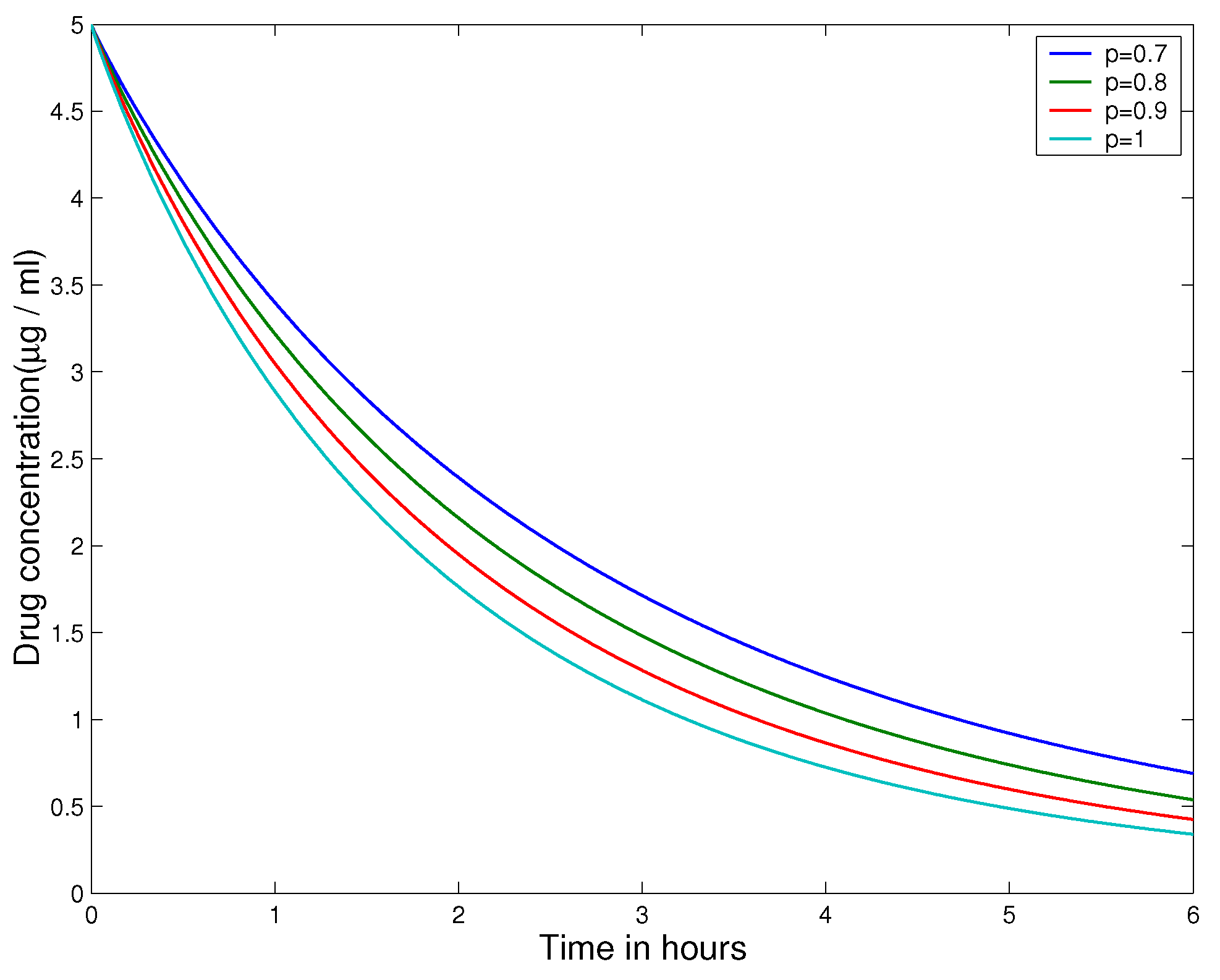
For the situation , the application of Theorem 3.10 gives that the solution of (14) is as follows:
Funding
This research received no external funding.
Institutional Review Board Statement
Not applicable.
Informed Consent Statement
Not applicable.
Data Availability Statement
Not applicable.
Conflicts of Interest
The author declares no conflicts of interest.
References
- M. Caputo, Linear models of dissipation whose Q is almost frequency independent-II, Geophysical Journal International 13 (1967) 529–539. [CrossRef]
- M. Caputo, M. Fabrizio, A new definition of fractional derivative without singular kernel, Progress Fractional Differention and Applications (2015) 73–85.
- A. Atangana, D. Baleanu, New fractional derivatives with non-local and non-singular kernel: theory and application to heat transfer model, Thermal Science 20 (2016) 763–769. [CrossRef]
- M. Al-Refai, On weighted Atangana-Baleanu fractional operators, Advances in Difference Equations 2020 (2020) 1–11. [CrossRef]
- K. Hattaf, A new generalized definition of fractional derivative with non-singular kernel, Computation 8 (2) (2020) 1–9. [CrossRef]
- K. Hattaf, A new mixed fractional derivative with applications in computational biology, Computation 12 (1) (2024) 1–17. [CrossRef]
- Y. Y Gambo, F. Jarad, D. Baleanu, T. Abdeljawad, On Caputo modification of the Hadamard fractional derivatives, Advances in Difference Equations (2014) 2014:10. [CrossRef]
- F. Jarad, T. Abdeljawad and D. Baleanu, Caputo-type modification of the Hadamard fractional derivatives, Advances in Difference Equations (2012) 2012:142. [CrossRef]
- R. Almeida, A. B. Malinowska, T. Odzijewicz, Fractional differential equations with dependence on the Caputo-Katugampola derivative, J. Comput. Nonlinear Dyn. 11(6) (2016) 061017. [CrossRef]
- K. Hattaf, A new generalized class of fractional operators with weight and respect to another function, Journal of Fractional Calculus and Nonlinear Systems 5 (2) (2024) 53–68. [CrossRef]
- S. T. M. Thabet, T. Abdeljawad, I. Kedim, M. I. Ayari, A new weighted fractional operator with respect to another function via a new modified generalized Mittag-Leffler law, Boundary Value Problems (2023) 2023:100. [CrossRef]
- T. Abdeljawad, D. Baleanu, On fractional derivatives with generalized Mittag-Leffler kernels, Advances in Difference Equations (2018) 2018:468. [CrossRef]
- A. Fernandez, D. Baleanu, Differintegration with respect to functions in fractional models involving Mittag-Leffler functions, SSRN Electron. J. (2018) 1–5.
- M. Al-Refai, A. Jarrah, Fundamental results on weighted Caputo-Fabrizio fractional derivative, Chaos, Solitons & Fractals 126 (2019) 7–11. [CrossRef]
- E. M. Lotfi, H. Zine, D. F. M. Torres and N. Yousfi, The power fractional calculus: First definitions and properties with applications to power fractional differential equations, Mathematics 10 (2022) 1–10. [CrossRef]
- S. M. Chinchole, Modified Definitions of SABC and SABR Fractional Derivatives and Applications, International Journal of Difference Equations (IJDE) 17 (1) (2022) 87–112.
- N. Aguila-Camacho, M. A. Duarte-Mermoud, J. A. Gallegos, Lyapunov functions for fractional order systems, Commun. Nonlinear Sci. Numer. Simulat. 19 (2014) 2951–2957. [CrossRef]
- M. A. Taneco-Hernández, C. Vargas-De-León, Stability and Lyapunov functions for systems with Atangana-Baleanu Caputo derivative: An HIV/AIDS epidemic model, Chaos, Solitons and Fractals 132 (2020) 109586. [CrossRef]
- C. Dai, W. Ma, Lyapunov direct method for nonlinear Hadamard-type fractional order systems, Fractal and Fractional 6 (2022) 1–23.
- K. Hattaf, On some properties of the new generalized fractional derivative with non-singular kernel, Mathematical Problems in Engineering 2021 (2021) 1–6. [CrossRef]
- R. Almeida, R.P. Agarwal, S. Hristova, D. O’Regan, Quadratic Lyapunov functions for stability of the generalized proportional fractional differential equations with applications to neural networks, Axioms 10 (2021) 1–14. [CrossRef]
- C. Vargas-De-León, Volterra-type Lyapunov functions for fractional-order epidemic systems, Commun. Nonlinear Sci. Numer. Simulat. 24 (2015) 75–85. [CrossRef]
- W. Ma, C. Dai, X. Li, X. Bao, On the kinetics of Ψ-fractional differential equations, Fractional Calculus and Applied Analysis 26 (2023) 2774–2804.
- H. Delavari, D. Baleanu, J. Sadati, Stability analysis of Caputo fractional-order nonlinear systems revisited, Nonlinear Dynam. 67 (2012) 2433–2439. [CrossRef]
- M. R. Rao, Ordinary differential equations, East-West Press: Minneapolis, USA, 1980.
- J. J. E. Slotine, W. Li, Applied Nonlinear Control; Prentice Hall: Englewood Cliffs, USA, 1991.
- G. Wang, K. Pei, Y.Q. Chen, Stability analysis of nonlinear Hadamard fractional differential system, Journal of the Franklin Institute 356 (12) (2019) 6538–6546. [CrossRef]
- K. Hattaf, On the Stability and Numerical Scheme of Fractional Differential Equations with Application to Biology, Computation 10 (6) (2022) 1–12. [CrossRef]
- Y. Li, Y. Q. Chen, I. Podlubny, Stability of fractional-order nonlinear dynamic systems: Lyapunov direct method and generalized Mittag-Leffler stability, Computers and Mathematics with Applications 59 (2010) 1810–1821. [CrossRef]
- T. R. Prabhakar, A singular integral equation with a generalized Mittag-Leffler function in the kernel, Yokohama Mathematical Journal 19 (1971) 7–15.
- S. M. Chinchole, A. P. Bhadane, A new definition of fractional derivatives with Mittag-Leffler kernel of two parameters, Communications in Mathematics and Applications 13 (1) (2022) 19–26. [CrossRef]
- F. Jarad, T. Abdeljawad, K. Shah, On the weighted fractional operators of a function with respect to another function, Fractals 28 (8) (2020) 1–12.
- J. Hadamard, Essai sur l’étude des fonctions données par leur developpment de Taylor, J. Math. Pures et Appl., Ser. (1892) 101–186. [CrossRef]
- A. A. Kilbas, Hadamard-type fractional calculus, J. Korean Math. Soc. 38 (6) (2001) 1191–1204.
- U. N. Katugampola, New approach to a generalized fractional integral, Applied Mathematics and Computation 218 (2011) 860–865.
- A. A. Kilbas, H. M. Srivastava, J. J. Trujillo, Theory and Applications of Fractional Differential Equations, North-Holland Mathematics Studies, Elsevier, Amsterdam, 2006.
- T. J. Osler, Leibniz rule for fractional derivatives generalized and an application to infinite series, SIAM J. Appl. Math. 18 (1970) 658–674.
- S. G. Samko, A. A. Kilbas, O. I. Marichev, Fractional Integrals and Derivatives: Theory and Applications, Gordon and Breach Science New York, 1993.
- C. Li, W. Deng, L. Zhao, Well-posedness and numerical algorithm for the tempered fractional ordinary differential equations, Discrete Contin. Dyn. Syst. Ser. B 24 (2019) 1989–2015. [CrossRef]
- M. M. Meerschaert, F. Sabzikar, J. Chen, Tempered fractional calculus, J. Comput. Phys. 293 (2015) 14–28. [CrossRef]
- D. Baleanu, A. Fernandez, On some new properties of fractional derivatives with Mittag-Leffler kernel, Communications in Nonlinear Science and Numerical Simulation 59 (2018) 444–462.
- F. Jarad, T. Abdeljawad, J. Alzabut, Generalized fractional derivatives generated by a class of local proportional derivatives, Eur. Phys. J. Spec. Top. 226 (2017) 3457–3471. [CrossRef]
- J. Alzabut, T. Abdeljawad, F. Jarad, W. Sudsutad, A Gronwall inequality via the generalized proportional fractional derivative with applications, J. Ineq. Appl. 2019 (2019) 1–12. [CrossRef]
- N. Sene, Stability analysis of the generalized fractional differential equations with and without exogenous inputs, Journal of Fractional Calculus and Applications 12 (9) (2019) 562–572.
- K. Hattaf, Stability of fractional differential equations with new generalized hattaf fractional derivative, Mathematical Problems in Engineering 2021 (2021) 1–7.
- N. Sene, Stability analysis of the fractional differential equations with the Caputo-Fabrizio fractional derivative, Journal of Fractional Calculus and Applications 11 (2) (2020) 160–172.
- F. Jarad, T. Abdeljawad, K. Shah, On the weighted fractional operators of a function with respect to another function, Fractals, 28 (8) (2020) 2040011. [CrossRef]
- M. Awadalla , Y. Y. Y. Noupoue, K. A. Asbeh, N. Ghiloufi, Modeling drug concentration level in blood using fractional differential equation based on Psi-Caputo derivative, Journal of Mathematics (2022) 1–8. [CrossRef]
Figure 1.
The graph of (15) for different values of order p.
Figure 1.
The graph of (15) for different values of order p.
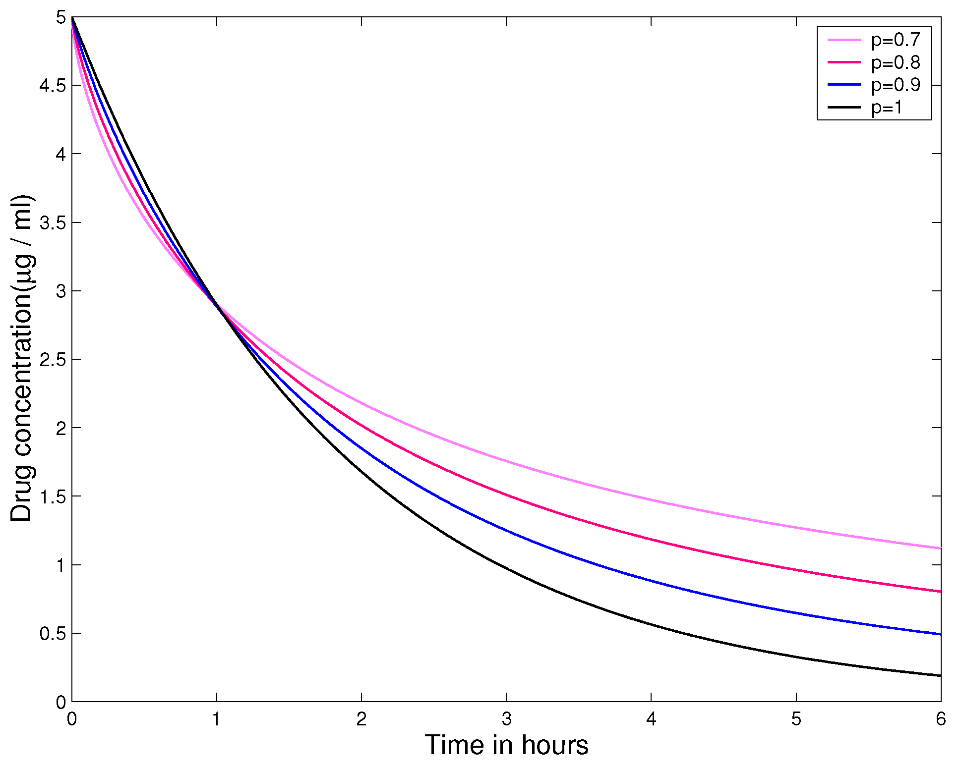
Figure 2.
The graph of (16) for different values of p with and .
Figure 2.
The graph of (16) for different values of p with and .
Disclaimer/Publisher’s Note: The statements, opinions and data contained in all publications are solely those of the individual author(s) and contributor(s) and not of MDPI and/or the editor(s). MDPI and/or the editor(s) disclaim responsibility for any injury to people or property resulting from any ideas, methods, instructions or products referred to in the content. |
© 2025 by the authors. Licensee MDPI, Basel, Switzerland. This article is an open access article distributed under the terms and conditions of the Creative Commons Attribution (CC BY) license (http://creativecommons.org/licenses/by/4.0/).
Copyright: This open access article is published under a Creative Commons CC BY 4.0 license, which permit the free download, distribution, and reuse, provided that the author and preprint are cited in any reuse.


