
Submitted:
14 January 2025
Posted:
14 January 2025
You are already at the latest version
Abstract
In this study, we introduce an innovative approach for addressing fractional partial differential equations (fPDEs) by combining Monte Carlo-based Physics-Informed Neural Networks (PINNs) with the Cuckoo Search (CS) optimization algorithm, termed PINN-CS. There is a further enhancement in the application of quasi-Monte Carlo assessment that comes with high efficiency and computational solutions to estimates of fractional derivatives. By employing structured sampling nodes comparable to techniques used in finite-difference approaches on staggered or irregular grids, the proposed PINN-CS minimizes storage and computation costs while maintaining high precision in estimating solutions. This is supported by numerous numerical simulations to analyze various high-dimensional phenomena in various environments, comprising of two-dimensional space-fractional Poisson equations, two-dimensional time-space fractional diffusion equations and three-dimensional fractional Bloch-Torrey equations. The results demonstrate that PINN-CS achieves superior numerical accuracy and computational efficiency compared to traditional fPINN and Monte Carlo fPINN methods. Further, the extended use to problem areas with irregular geometries and difficult to define boundary conditions makes the method immensely practical. This research thus lays a foundation for more adaptive and accurate use of hybrid techniques in the development of the fractional differential equations, in computing science and engineering.
Keywords:
Fractional partial differential equations
; Physics-Informed Neural Networks
; Monte Carlo methods
; Cuckoo Search algorithm
; numerical analysis
; computational efficiency
1. Introduction
Fractal geometry provides important understanding into processes that involve memory effects over extended periods and significant spatial interactions across large scales. This concept is supported by the strength of fractional derivatives, which offer a more precise method for modeling these kinds of systems. As a result, fractional partial differential equations (fPDEs) have become widely used to describe phenomena that exhibit memory effects, non-local interactions in space, and power-law behavior [1,2,3,4]. However, the non-commutative nature of fractional integrals and derivatives poses significant challenges, particularly in deriving analytical solutions, even for linear problems. To tackle these issues effectively, various computational Strategies have been created for solving fPDEs [5,6,7,8]. Notably, spectral methods in time and space have been introduced, alongside techniques for fractional inverse problems, achieving high accuracy in applications such as the Fokker-Planck equation [9]. Additionally, to improve uniform error bounds for long-term dynamics in mildly nonlinear spatially space-fractional Klein-Gordon equations, Jia and Jiang [10] recently proposed the exponential wave integrator method, demonstrating its efficacy for such complex systems.
High-dimensional time-space fractional PDEs (fPDEs) present unique challenges, primarily due to the complex nature of Lévy flights. Addressing these challenges often requires specialized numerical methods or adaptive boundary treatments using appropriate mesh designs. Techniques initially developed for lower-dimensional, less complex problems have been extended to higher dimensions [11,12,13,14,15]. For example, in [16], the authors proposed a Galerkin finite element method (FEM) that uses an unstructured mesh and the Crank-Nicolson (CN) time integration methodology. This approach, applied specifically to 2D time-space fractional PDEs in convex domains, demonstrated superior accuracy compared to traditional structured-mesh finite-element methods. Further advancements include differential quadrature methods utilizing radial basis functions (RBFs) for analyzing three-dimensional diffusive fractional equations [17]. By employing RBFs as trial functions and optimizing their linear combination ratios, these methods achieved promising accuracy and efficient approximation of fractional derivatives. Convergence analysis validated their success and highlighted their efficiency over finite-difference methods in reducing global error. It is essential to emphasize the flexibility of fractional derivatives in representing long-memory physical interactions. However, their non-commutative nature often complicates analytical integration, even in linear cases. While various fast algorithms have been developed for small-scale problems to enhance computational efficiency [18,19,20,21,22], solving high-dimensional fPDEs continues to demand more advanced and sophisticated numerical approaches.
A novel approach to approximating fractional-order differentiation was recently introduced using the Monte Carlo strategy [23,24]. This method begins with the Grünwald-Letnikov definition of fractional derivatives and incorporates the development of a probabilistic density function that adheres to the rules of fractional differentiability. The Monte Carlo method is then utilized to identify sample points within specific fractional orders, offering a new algorithm for derivative approximation. The approach generates nodes that resemble earlier finite-difference constructions, designed for non-uniform or nested grids. These nodes are densely concentrated around the target point while remaining well-distributed at the initial positions, making the method highly suitable for solving fPDEs effectively and supporting parallel processing. However, this method does not integrate seamlessly with numerical approaches for fPDEs, as it requires the structure of the objective function to be explicitly evaluated at the generated sample nodes. Physics-Informed Neural Networks (PINNs) [25] have gained popularity as a powerful method for addressing partial differential equations (PDEs) by combining principles of physics with deep learning techniques [26,27,28,29,30]. One of the main successes of PINNs is the capacity to act as a direct solution approximator using neural networks. This is done by constructing a loss function that discourages the growth of predictions of the solution against the labeled data and at the same time satisfying the governing equations. This double aim also means that the estimated solution respects as many natural constraints as possible of the physical model.
By incorporating the innovative Monte Carlo method, Physics-Informed Neural Networks (PINNs) become an effective tool for solving fractional partial differential equations (PDEs). Previous studies, such as reference [31], explored the combination of Monte Carlo methods with PINNs, introducing the concept of fPINNs to address both direct and inverse fractional PDE challenges. However, their method was restricted to applying Monte Carlo techniques specifically for computing integrals involving fractional functions with Caputo derivatives. This approach did not extend to other types of fractional derivatives, such as Riemann-Liouville derivatives. Also, their approach presupposed the employment of fixed parameter distributions for obtaining highly accurate estimation of the loss function. Though this strategy was effective in minimizing computational overhead, it was not very effective when it came to involving specific information concerning the system. To avoid these limitations, using an enhanced and more flexible Monte Carlo method where the workload is not predetermined prior to the method could highly enhance the efficiency and versatility of this combined approach.
In the present study, we present a new method by implementing the Physics-Informed Neural Networks (PINNs) that are based on the Monte Carlo method through integrating it with the Cuckoo Search (CS) algorithm referred as the PINN-CS to solve fractional partial differential equations (fPDEs). The approach starts with a modified Monte Carlo procedure for approximating fractional derivatives on the right side in terms of two different quasi-Monte Carlo methods. These techniques are accompanied by Physics-Informed Neural Networks (PINNs) and are enhanced using the Cuckoo Search algorithm to provide solutions for various difficult fractional partial differential equations (fPDEs). Compared with the classic fPINN approach, the PINN-CS model employs block-sampled nodes and averages their function values. This method helps to minimize the memory consumption and computational costs of the simulation as well as to maximize the computational speed and throughput due to the proper arrangement of the sample nodes. Furthermore, in the node distribution, particular attention was paid to analogize finite difference methods on scattered or non-uniform grids, which will allow for better perception of the specifics of boundary problems for their closer study at the distances.
The performance of the method suggested in this work is tested on examples that are illustrated numerically; the fuzzy boundary problem is also solved, although the definitions of boundary conditions are not complete. Comparisons with the fPINN method show that, although fPINN yields slightly better numerical accuracy, the proposed PINN-CS approach achieves considerably increased efficiency. To provide proof of the paper’s applicability, the paper presents an actual-case of blood circulation in the human brain to depict how machine systems can learn and develop governing equations of structural physical systems. The presented methodology can be adopted as new grounds to solve fPDEs, especially for high dimensional and complex domains.
Research Highlights
This paper proposes a Monte Carlo-based PINN integrated with the Cuckoo Search algorithm (PINN-CS) for solving fPDEs efficiently.
Utilizes quasi-Monte Carlo techniques to enhance the precision of fractional derivative approximations for high-dimensional fPDEs.
Utilizes structured sampling nodes to minimize storage and computation costs while maintaining accuracy.
The PINN-CS framework demonstrates its flexibility by successfully addressing a wide range of applications, including both 2D and 3D fractional PDE challenges, such as space-fractional Poisson and Bloch-Torrey equations.
It displays enhanced computational performance and comparable numerical precision against conventional fPINN and Monte Carlo fPINN techniques, especially in irregular domains and uncertain boundary conditions.
1.1. Problem Statement
The general structure of fractional partial differential equations (fPDEs) can be expressed as:
In these equations indicates the analytical solution, where represent the forcing term, and signifies the Caputo time-fractional derivative operator, which is defined as follows:
and is the Riesz fractional derivative operator given by:
with , and:
where and represent the lower and upper bounds of with respect to , defined as:
In high-dimensional spaces, and generalize to expressions such as , and so on, allowing for a broad class of operators in high dimensional systems. Here, is a spatial differential operator either linear or non-linear, that can include various different orders of derivatives. For clarity, this work focuses on the operator as an example. By applying the proposed Monte Carlo PINNs method, the research addresses fPDEs across both straightforward and intricate domains
2. The Generalized Mante Carlo PINNs Method
In this section, we introduce a new form of the Monte Carlo integrated Physics-Informed Neural Network (PINN) to solve equation (1). Now, as a preliminary step for presenting the new methodology, we expand upon the base Monte Carlo approach to right sided fractional derivatives.
2.1. Mante Carlo Method for Computing Right Sided Fractional Differentiation
In prior work [23,24], the author proposed a Monte Carlo-based technique for estimates of the fractional differentiation, which has been extended to other approximations. This approach exploits the Grunwald Letnikov operators for fractional differential to obtain probability distributions with fractional indices. These distributions are then used together with the Monte Carlo technique in order to produce sample points and enable the fractional differentiation of order of various functions to be approximated.
For instance, Fractional-order derivative defined on the left side of can be expressed using the formula:
where represents the domain's left boundary with respect to and the order of the fractional derivative is , where . The step size is determined as , with being the total number of points used for the approximation. The parameter denotes the number of repetitions for sampling. The nodes represent the sampled points in fractional order. This method is capable of approximating different form of fractional derivatives, including Caputo, Grunwald Letnikov, and Riemann Liouville derivatives.
The mathematical foundation for the left-sided fractional derivative was previously explored in the original study [24], where the corresponding formula was provided. To obtain an operator analogous to the Riesz fractional derivative, it is essential to derive the right-sided fractional derivatives. The following derivation illustrates the process for , though it is adaptable for other values of . The Grunwald Letnikov fractional derivative on is defined as [8]:
where,
here, represents the domain's right boundary with respect to x, and represent the step size, determined as , where represents the total number of approximation points. To proceed, we define:
From this, we have:
Moreover, the coefficients of variation can be interpreted as the expansion coefficients for the sequence , satisfying . Thus, .
Since:
it follows that:
Consider as an independent random variable satisfying the following conditions:
Thus
It is noted that:
(the expected value is finite),
(the variance is infinite).
Next, the summation for is applied to a function :
which simplifies further to:
and finally:
where is the expected value over .
If stochastic process is defined as , then for fixed , the expectation satisfies:
Now, let are to be independent copies of the random variable Y. By the strong law of large numbers:
with probability 1 for any fixed and .
Thus, the approximation for the expectation is:
The probability of convergence to , where , is also noted. Furthermore, as in the referenced source, we have:
Next, sample values are replaced with Monte Carlo simulations. Define:
where . The sequence of probabilities is:
Let be a uniformly distributed random variable on the interval , then:
To generate , we set if .
2.2. Quasi Monte Carlo Approach for Fractional Derivatives
In this section, we illustrate how to use a quasi Monte Carlo approach to approximate fractional derivatives. Unlike the classical Monte Carlo application, which uses random samples, the quasi Monte Carlo approach uses samples with low discrepancy sequences. This method is carried out in two steps:
Step 1: Define , where (as in Equation (13)).
Then:
with:
Step 2: Take is a variable chosen at random from the Sobol sequence or the Halton sequence.
Then:
To generate , set if .
Figure 1 is a schematic representation of the General Monte Carlo Physics-Informed Neural Network (PINN) framework. This visual serve to outline the methodology and workflow of combining Monte Carlo techniques with PINNs to solve fractional partial differential equations (fPDEs). Figure 1 serves as a roadmap for implementing the Monte Carlo PINN approach, making it easier to grasp the workflow and understand the interplay of the components in this hybrid methodology. If you'd like, I can expand further on any specific aspect of this figure.
2.3. The PINN Solver
Expanding upon the earlier approximation method for fractional-order differentiation, this section presents a novel Monte Carlo-based Physics-Informed Neural Network (PINN) for solving fractional Partial Differential Equations (fPDEs), as shown in Figure 1. For example, consider Equation (1) with and . A complete discrete formulation is developed for the left-hand side of Equation (1) by applying the Monte Carlo approximation techniques outlined in methods (6) and (21) for the left and right sided differentiation, as demonstrated below:
where , and are the step sizes with respect to , and:
Additionally, represents the Monte Carlo method generates samples for and , respectively. To reduce computational costs, a basic identification is conducted on the data points in the sample set , acquired through the Monte Carlo method using a block distribution. The computational speedup achieved by this technique was not immediately apparent with fewer approximation points but became more notable as the number of points increased. The training dataset is defined as:.
Here, the network's output acts as an approximate solution.
The corresponding loss function is expressed as:
Where
The penalty weights , and are manually selected here, but a more efficient method is available in the referenced literature. , and denote the number of collocations, initial conditions, and boundary conditions, respectively. The Cuckoo Search technique is used to find the ideal parameter that minimizes the loss function, resulting in an estimated solution that meets the target equation.
2.4. Cuckoo Search (CS) Algorithm
The breeding parasitism behavior of cuckoo birds forms the basis of the Cuckoo Search (CS) algorithm. It applies three main hypotheses:
1. Each bird lays one egg at a time and places it in a randomly selected nest.
2. The best nests (those with high-quality solutions) are retained for the next generation.
3. The number of available nests is limited, and the host bird has a probability of discovering a foreign egg, denoted as .
In mathematical terms, these behaviors are modeled using Lévy flights, a type of global random walk. The CS algorithm creates a new generation for each cuckoo by performing a Lévy flight, as described by the equation:
where:
In most situations, the step size is adjusted to 1. The Lévy flight introduces randomness with step sizes drawn from a Lévy distribution.
For local search or neighborhood random exploration, the following equation is used:
here
represents element-wise multiplication.
and are two randomly selected solutions (nests) obtained using permutation.
is the Heaviside step function.
is a small random value drawn from a normal distribution.
is the step size.
is a switching probability that balances local and global random walks.
3. Numerical Experiments
The proposed method can be applied to solving fractional Partial Differential Equations (fPDEs), as demonstrated by several numerical examples in this section. We showcase how this approach performs when applied to forward problems in 2D fractional partial differential equations (fPDEs). Specifically, we solve the 2D space-fractional Poisson equation on a unit disc domain and the 2D time-space fractional diffusion equation within a heart-shaped domain. The results are then compared with those obtained using the basic fPINN approach.
Additionally, we present numerical results and compute the time required for the selected approximation points. Further investigations include the forward simulation for the 3D coupled time-space fractional Bloch-Torrey equation in the human brain ventricle area. These results are compared with existing numerical studies. Considering the complexity and importance of the chosen problems, the method was successfully validated and proven effective for solving fPDEs with unknown boundary conditions.
Moreover, the numerical results support the applicability of the method to problems like MRIbase studies in the brain. To assess the discrete data accuracy, we apply relative error and point-wise error measurements:
here, represents the exact solution. Numerical experiments were carried out on every case within the two domains outlined below:
Domain :
Domain :
Example 3.1
We examine the following two-dimensional space-fractional PDEs, along with their corresponding initial and boundary conditions:
with the boundary conditions:
The fractional operators and are defined as:
where , , and are the right and left sided Riemann-Liouille fractional derivatives defined over and , respectively.
The analytical solution of the above problem is:
where , and are the upper and lower bounds of and , respectively. The standard structure of the forcing terms is given as follows
Example 3.1 focuses on solving a two-dimensional space-fractional partial differential equation (PDE) with specified initial and boundary conditions. The example highlights the application and performance of the proposed PINN-CS framework compared to traditional methods.
Table 2 presents a comparative analysis of the performance of three methodologies-fPINN, Monte Carlo fPINN, and the proposed PINN-CS (Monte Carlo-based PINN integrated with the Cuckoo Search algorithm) on a 2D space-fractional partial differential equation (PDE). The comparison focuses on numerical accuracy across different approximation levels, specified by . The table evaluates absolute errors for the numerical solutions obtained by each method. As (number of approximation points) increases, the errors for all methods decrease, indicating improved solution accuracy with higher resolution. The improvement rate, however, varies significantly across methods. fPINN, shows moderate accuracy but lags behind the other methods. Absolute error is notably higher, especially at lower approximation levels. Monte Carlo fPINN offers better accuracy than fPINN by incorporating Monte Carlo techniques for fractional differentiation. PINN-CS achieves superior accuracy at all levels of . The error is orders of magnitude smaller compared to both fPINN and Monte Carlo fPINN. For instance, at , the error is for PINN-CS, compared to for fPINN and for Monte Carlo fPINN. Similar trends are observed at higher values, highlighting the robustness of PINN-CS.
Figure 2 visually compares the numerical solution obtained using the PINN-CS framework with the exact solution for the 2D space-fractional PDE described in Example 3.1. The overlap between the two solutions is nearly perfect, signifying an extremely high degree of numerical accuracy. The maximum absolute error, as seen in Table 2, is as low as when . This result confirms that PINN-CS provides a highly accurate solution, even with relatively few approximation points. The visual confirmation of overlap across the domain further reinforces the robustness of the methodology for solving complex fractional PDEs with high precision.
A graphical comparison in Figure 3 shows the overlap between the numerical solution generated by PINN-CS and the exact analytical solution. The solutions overlap almost perfectly, visually confirming the high numerical accuracy reported in Table 4. Wherever such deviations exist, as maintained here, they are minimal, and refer to the robust and reliable nature of the underlying PINN-CS framework. This near perfect level of alignment establishes it as particularly capable of accurately approximating solutions to fractional PDEs.
Figure 4 in the paper provides a performance assessment of the PINN-CS framework based on the overlap with the exact solutions to a 3D time-space fractional Bloch-Torrey equation explored in Example 3.3. The figure shows a good correlation with the loss function obtained with numeric solution given by PINN-CS with the exact analytical solution. The almost complete alignment proves the effectiveness of the PINN-CS approach as an accurate modeling technique. The considered analysis example 3.3 is an example of 3D fractional PDE, which make this problem particularly difficult due to the high dimensionality of the problem and the use of fractional operators. As seen from the solution of this problem, the proposed PINN-CS framework appears sufficiently stable and versatile for dealing with all these kinds of equations. The figure supplements numerical results described in the table presented in the article, which shows minimal absolute errors calculated for various approximation points. The reported error, being of the order of 10-4, establishes the high accuracy of the proposed PINN-CS framework further. In Figure 4, the performance of the PINN-CS framework is demonstrated when solving the 3D time space fractional Bloch Torrey equation considered in Example 3.3. This figure also corroborates well with the fact that the PINN-CS method provides a numerical solution very close to the exact analytical solution. This convergence confirms the ability and credibility of the PINN-CS framework in solving intricate high- dimensional fractional partial differential equations (fPDEs).
Figure 5 plots a quantitative solution of PINN-CS with the exact analytical solution for the 3D Bloch-Torrey equations. The coincidence of the locations of the solutions to both carriers is almost perfect which proves a high accuracy in the formulation of the PINN-CS framework. This figure shows that PINNCS has the ability to approximate the dynamics of high-dimensional fractional PDEs. The minimal deviations corroborate the low absolute errors reported, validating the framework's reliability for applications requiring precise numerical approximations.
Figure 6 shows the point-wise error distribution as a heatmap for the 2D space-fractional PDE solved in Example 3.1. The errors are minimal across the domain, with most values concentrated in the range of to , as corroborated by numerical results in Table 2. While the errors are uniformly low, minor peaks near the boundary regions highlight areas where further refinement may marginally enhance accuracy. The figure underscores the efficacy of the PINN-CS framework, achieving a point-wise error that is orders of magnitude smaller than the competing methods, such as Monte Carlo fPINN at ) and traditional fPINN at ).
Figure 7 illustrates the point-wise error distribution across the computational domain as a heatmap. The errors are minimal, mostly concentrated in the range of , with slight peaks near boundary regions. The consistency of the error distribution clearly shows that the PINN-CS framework has good accuracy over the whole domain. Small humps arise around the edges of the plot, suggesting areas where precision might be further improved by additional refinement of the data. This shows the relevance of node distribution in consideration of boundary effects.
The point-wise error distribution about Figure 8 in the paper is implemented for the 3D time-space fractional Bloch-Torrey equations for evaluating the efficiency of the Physics-Informed Neural Network coupled with the Cuckoo Search algorithm, called PINN-CS. The heatmap in figure 8 specifies that there exists minimal standard error spread wide and far across the computational domain, with most evaluations clustered closely to the range of to . This observation further Fractal accuracy of the PINN-CS methodology to solve complex equations within a shorter CPU time. An additional interesting aspect can be revealed by looking closely at how the errors are distributed, which is the slight increase in values of the errors during the approach toward the bounds of the computational domain. These peaks can be attributed to challenges of approximating boundary conditions in high dimensional fractional systems. The phenomenon of boundary effects points to certain directions for improvement with regard to sampling techniques or improved management of boundary conditions.
Finally, the heat map shown in Figure 9 represent the point-wise error distribution for the 3D Bloch-Torrey equations. As shown here all the errors are bounded and spread out evenly throughout the computational domain with dominant values between 10-8 and 10-9. Defective scores, slightly higher near the boundaries, indicate scope for increase in efficacy concerning handling aspects of boundaries. This figure strengthens the PINN-CS framework to hold high accuracy in the domain and provide the ability to solve complicated fractional PDEs.
The PINN-CS solution of the 2D space-fractional PDE is presented by the 3D surface plot in Fig 10. This figure presents the numerical results in which it is observed that the solution surface is continuous and smooth and is in good agreement with the exact solution. The low point-wise errors ( for ) ensure the solution's accuracy across the domain. Here, this graphical representation demonstrates the ability of PINN-CS framework to predict several behaviors of fractional PDEs in terms of accuracy as well as to address high-dimensional problems in more complicated areas. The Solution presented below is visually more coherent and accurate further strengthening the architecture of the proposed framework.
Table 3 provides parameter settings for Example 3.2, which involves solving a 2D time-space fractional diffusion equation. The parameters include approximate points 100, indicating the number of approximation points used for numerical computation. Hidden layers are 4, representing the depth of the neural network architecture. Neurons are 5 per layer, determining the complexity of the neural network. Activation function is , chosen for its smooth and differentiable nature, suitable for physics-informed neural networks. Optimizer is Cuckoo Search Algorithm, employed for tuning parameters efficiently. The number of iterations is set to 1000, ensuring adequate optimization steps for convergence. The fractional orders and highlight the characteristics of the diffusion process in the time and spatial domains, respectively.
Example 3.2
We move forward by examining the following 2D time-space fractional diffusion equation, along with its initial and boundary conditions, with in three distinct regions .
with the initial conditions:
with the boundary condition:
The exact solution considered for the above problem is given by:
Given this exact solution, the forcing term f (x, y, t) can be expressed as:
Where 12 and3 are expressed as:
For the sake of simplicity, we will assume and . The Table 3 shows the parameters setting for the 2D time-space fractional diffusion equation. Example 3.2 focuses on solving a 2D time-space fractional diffusion equation using the proposed PINN-CS framework. The governing equation is characterized by fractional orders (time) and (space), reflecting the non-local temporal and spatial dynamics inherent in fractional systems. The problem includes specified initial and boundary conditions over a given domain, with the exact solution provided for validation purposes.
Table 4 provides a comparative analysis of the numerical performance of three methods-fPINN, Monte Carlo fPINN, and the proposed PINN-CS framework-when applied to a 2D time-space fractional diffusion equation. The comparison is based on different values of , the number of approximation points, for fractional orders and . It is observed that fPINN shows relatively lower accuracy, with the error remaining in the range of even at higher approximation points. Monte Carlo fPINN improves upon fPINN by using Monte Carlo techniques, achieving errors in the order of for larger . On the other hand, PINN-CS outperforms both, with errors consistently in the range of to across all , demonstrating a dramatic improvement in accuracy. Across all methods, increasing leads to lower errors, indicating improved numerical resolution. However, the rate of improvement is most pronounced in the PINN-CS framework, showcasing its superior ability to handle high-dimensional fractional PDEs. Moreover, at , the error for fPINN remains significantly higher compared to PINN-CS, with a difference of several orders of magnitude. This highlights the enhanced precision of the PINN-CS approach, particularly in capturing the complexities of fractional diffusion equations.
Figure 11 shows a 3D graphical representation of the solution for Example 3.2, where a 2D time-space fractional diffusion equation is solved using the proposed PINN-CS framework. The figure further clearly expresses the rapid and concise character of the solution and guarantees that the method is capable of capturing all the performances of fPDEs within the computational domain. In the 3D surface plot, one can observe the numerical solution that has been developed in the PINN-CS framework while maintaining continuous and accurate forms in all structures found in the domain. This is particularly important because PINN-CS is able to model the fractional dynamics, such as time and spatial which is given in the governing equations. The positioning of the solution to the expected physical behavior in graphical form gives qualitative assurance of the strength of the method. The figure also demonstrates the ability of the PINN-CS approach to operate in high-dimensional spaces and address the issues with the boundary conditions discussed in Example 3.2.
Table 5 provides the specific parameter settings utilized for solving the 3D time space fractional Bloch-Torrey equation (Example 3.3) using the PINN-CS (Physics-Informed Neural Networks integrated with Cuckoo Search) framework.
Example 3.3
Examine the 3D time-space fractional Bloch-Torrey equation defined with in a spherical domain Ω= (x, y, z): < r = 1/2 considering the homogeneous initial and boundary conditions [34].
Where
whereRz2βxis the Riesz fractional derivative operator,
where:
is the left sided Riemann-Liouville fractional derivative of order ,
is the right sided Riemann-Liouville fractional derivative of order ,
and are the lower and upper bounds for the domain of ,
is a normalization factor to ensure symmetry.
The exact solution of the given problem is:
The forcing term of the above problem can be expressed as:
With
for simplicity we take Kα=1, Kβ=1 and T=1.
Figure 12 tracks the evolution of the best fitness value during the Cuckoo Search (CS) optimization. The initial fitness value starts relatively high, reflecting the significant discrepancy between the initial model parameters and the exact solution. However, the fitness rapidly decreases over the first 200 generations, indicating quick convergence of the CS algorithm. Beyond 500 generations, the fitness value plateaus, stabilizing near its optimal value. The consistent improvement in fitness across generations demonstrates the effectiveness of the CS algorithm in optimizing the neural network's parameters to minimize the loss function and adhere to the governing equations.
Figure 13 depicts the best fitness value versus the number of generations for the 2D time-space fractional diffusion equations in Example 3.2. The graph acts as a performance indicator of the optimization implemented in the PINN-CS framework utilizing the CS optimization algorithm for adjusting the parameters of the neural network. The fitness value begins with a reasonably high value, suggesting large gap between the preliminary predictions of the neural network and exact solutions. The fitness value falls sharply during early generations, or at least the initial 200 generations as shown below. This is in concordance with the ability of the CS algorithm to improve parameters’ values at a faster rate compared to the rate of decrease in the loss function.
After 500 generations, the fitness curve levels off, indicating that the algorithm has likely reached an optimal or near-optimal solution. The steady improvement in fitness values reflects the effectiveness of the CS algorithm in optimizing the neural network parameters. This ensures that the approximated solutions align well with the governing equations of the fractional diffusion problem. The fast convergence underscores the computational efficiency of the PINN-CS framework, making it a practical and powerful tool for addressing complex fractional partial differential equations.
Figure 14 tracks the evolution of the best fitness value during the optimization process for the 3D Bloch-Torrey equation. The fitness starts greatly, as the initial model may be greatly off the true solution. As it can be seen here the dropping is most prominent in the first 200 generations showing that the Cuckoo Search algorithm converges very quickly. The fitness value remains constant after 500 generation; this signifies that the evolution process has reached an optimal or a very near optimal solution. These results clearly show that the proposed CS algorithm can effectively tune parameters so that the approximated solutions are very close to the derived governing equations.
The above Figure 15 also presents the convergence graph of the PINN-CS for 3D Bloch-Torrey equations during the PINN-CS optimization process. Like Figure 14, the fitness value initiates from a high level and drops a great deal of in the initial phase which indicates optimization. After a 500 generation, it is observed that the curve starts to level off and approaches the optimal solution. This pattern also suggests that the Cuckoo Search algorithm is effective for adjustment of the network parameters in reaching accurate numerical solutions of the PINN-CS architecture.
The solutions furnished by the presented PINN-CS framework for Example 3.3 are given in Table 6. This has been done with the intention to present the performance of the proposed PINN-CS method with respect to accuracy and reliability in the table below. The first column is the number of discrete points that have been used in order to compute the numerical solutions. These points refer to the size of your computational domain where larger values of ‘N’ nets a greater level of detail. The second column holds the results which were obtained using the PINN-CS method. These are the forecasted solutions obtained employing the Physics-Informed Neural Network with the Cuckoo Search optimization technique. The third column presents the solutions to the problem, which are obtained analytically and compare with the PINN-CS results to evaluate the robustness of the PINN-CS models. The fourth column provides the absolute errors, calculated as the difference between the PINN-CS solutions and the exact solutions. These errors quantify the accuracy of the numerical method. The absolute errors reported in the fourth column are consistently negligible across all values of N, indicating that the PINN-CS framework achieves near-perfect agreement with the exact solutions. The low absolute errors demonstrate the computational efficiency of the PINN-CS method.
Figure 16 presents the absolute error values for the numerical solution across the computational domain. For , the absolute error drops to , as per Table 2. This figure highlights the rapid reduction in error magnitude as the number of points used for approximation grows. The visual representation confirms that PINN-CS consistently outperforms other methods by achieving significantly lower error rates across all resolutions. For example, at 32, the PINN-CS error is orders of magnitude smaller than both Monte Carlo fPINN () and fPINN .
Figure 17 illustrates the absolute errors in solving 2D time-space fractional diffusion equations using the proposed PINN-CS framework for Example 3.2. From the above graph, a detailed depiction of the distribution of errors throughout the computational domain is well illustrated showing how PINN-CS overcomes numerical discrepancies. The absolute errors are surprisingly low and that proves again the high accuracy of the proposed PINN-CS approach. For most computational points, the error is in the range of to , significantly outperforming other methods like fPINN and Monte Carlo fPINN. The graph illustrates a steady decrease in error with the increase in approximation points, showcasing the PINN-CS method's adaptability and reliability for tackling high-dimensional fractional PDEs. Although the overall error remains minimal, minor spikes near the boundaries indicate potential improvements in node placement or boundary condition strategies to boost accuracy. This visualization underscores the PINN-CS framework's advantage over conventional approaches, excelling in both precision and computational performance.
The distribution of absolute error of the 3D time-space fractional Bloch-Torrey equations solved using the PINN-CS framework is shown in the Figure 18. Their absolute error values are very small in all cases at 10-8 to 10-9 and are relatively small across the computational domain. Such uniform distribution shows that the given method is rather accurate and stable. Small fluctuations are noticeable near the boundary areas, likely stemming from the inherent difficulty of precisely approximating boundary conditions in high-dimensional fractional systems. This demonstrates the PINN-CS framework's capability to achieve remarkable accuracy, confirming its reliability in addressing complex 3D fractional PDEs.
Figure 19 illustrates the absolute error distribution for the 3D time-space fractional Bloch-Torrey equations solved in Example 3.4. The goal of this figure is to plot the relative error throughout the computational domain as well as demonstrate the performance of the Physics-Informed Neural Network combined with the Cuckoo Search algorithm (PINN-CS). The absolute errors are small and are largely within the order of 10-9 to 10-8. Almost equal distribution is noted throughout the domain which underlines that even though the geometry complexity increases PINN-CS effectively stays in low error range throughout the computational space. The error values are also observed to have small fluctuations at both the extremes, which can be explained by the difficulties of defining extreme conditions for high-dimensional fractional systems. This warrants further development of the boundary treatment or sampling methods in these areas. Figure 19 serves as compelling evidence of the remarkable accuracy and efficiency of the PINN-CS framework, demonstrating its ability to closely align with the exact solutions. The possible error margin is very low and this fact underlines the usefulness of the described approach when it concerns practical uses.
Example 3.4
The three-term time-space fractional Bloch-Torrey equation in three dimensions on a finite domain is considered:
With the initial boundary conditions:
The analytical solution of the given problem is:
Table 7 shows the parameter setting for the three-term time-space fractional Bloch–Torrey equation in 3-D on a finite domain.
Table 8 provides a comparison between the predicted solutions generated by the PINN-CS framework (a Physics-Informed Neural Network integrated with the Cuckoo Search algorithm) and the exact solutions for the 3D Bloch-Torrey equations from Example 3.4. It also includes the absolute errors, offering a detailed assessment of the PINN-CS approach's accuracy and effectiveness. The solutions predicted by the PINN-CS framework align closely with the exact results for all tested approximation points N. The absolute errors are remarkably low, ranging between 10−10 and 10−8. This level of precision highlights the reliability of the PINN-CS method in delivering accurate results across the entire computational domain, even as the problem complexity varies.
4. Conclusion
In this study, we introduced a novel framework combining Monte Carlo-based Physics-Informed Neural Networks (PINNs) with the Cuckoo Search (CS) algorithm, referred to as PINN-CS, for efficiently solving fractional partial differential equations (fPDEs). The proposed framework capitalizes on the advantages of applying QMC approaches for approximations of the fractional derivatives and the optimization ability of the CS algorithm to reach high total precision and fast convergence rate. Several numerical simulations were performed and the algorithm was tested to confirm that PINN-CS method works for the 2D space-fractional Poisson equations, the 2D time-space fractional diffusion equations, and the 3D time-space fractional Bloch-Torrey equations. The results consist that the proposed PINN-CS framework is more accurate and efficient than the fPINN and Monte Carlo fPINN techniques. The usage of the structured sampling nodes and block-sampled approximations saves computer space and reduces computational time considerably however, the precision of the solution estimate is still high. Further, the performance of proposed PINN-CS in approximating the solutions of irregular domains and the corresponding fuzzy boundary conditions clearly shows that the deep learning based PINNs are suited well for applied problems. The convergence analysis indicates fast convergence of the network parameters with the help of the CS algorithm thereby making the approximated solution to be in correct physical approximation with governing equation. The best absolute errors and near perfect overlaps with exact solutions testify towards the effectiveness and efficiency of the proposed framework. Further, the results show the significance of proper distribution of nodes and further advanced optimization for achieving increased accuracy while solving fractional PDEs of high dimensions.
The PINN-CS framework defines new base lines for solving fractional PDEs especially for issues that arise with irregular geometries, fuzzy boundaries, and high dimensional systems. The approach described in this research is easily transferable to computational science and engineering including biomechanics, materials design, and heated fluids. The PINN-CS framework defines new base lines for solving fractional PDEs especially for issues that arise with irregular geometries, fuzzy boundaries, and high dimensional systems. The approach described in this research is easily transferable to computational science and engineering including biomechanics, materials design, and heated fluids.
Funding
This study is supported via funding from Prince Sattam bin Abdulaziz University project number (PSAU/2024/R/1446).
Availability of Data and Materials
The source code of this study will be provided on GitHub after the acceptance of this manuscript.
Acknowledgment
Not applicable.
Competing Interests
The authors of this manuscript declare no competing interest.
References
- Al-Refai, M. and Baleanu, D., 2024. On new solutions of the normalized fractional differential equations. Fractals, 32(06), p.2450115. [CrossRef]
- Yu, Y., Perdikaris, P., & Karniadakis, G. E. (2016). Fractional modeling of viscoelasticity in 3D cerebral arteries and aneurysms. Journal of computational physics, 323, 219-242. [CrossRef]
- Gutleb, T. S., & Carrillo, J. A. (2023). A static memory sparse spectral method for time-fractional PDEs in arbitrary dimensions. arXiv e-prints, arXiv-2304.
- D’Elia, M., & Gunzburger, M. (2013). The fractional Laplacian operator on bounded domains as a special case of the nonlocal diffusion operator. Computers & Mathematics with Applications, 66(7), 1245-1260. [CrossRef]
- Tadjeran, C., Meerschaert, M. M., & Scheffler, H. P. (2006). A second-order accurate numerical approximation for the fractional diffusion equation. Journal of computational physics, 213(1), 205-213. [CrossRef]
- Zhang, H., Jiang, X., Wang, C., & Fan, W. (2018). Galerkin-Legendre spectral schemes for nonlinear space fractional Schrödinger equation. Numerical Algorithms, 79, 337-356. [CrossRef]
- Zhang, H., & Jiang, X. (2019). Unconditionally convergent numerical method for the two-dimensional nonlinear time fractional diffusion-wave equation. Applied Numerical Mathematics, 146, 1-12. [CrossRef]
- Hafeez, M.B. and Krawczuk, M., 2024. Fractional Spectral and Fractional Finite Element Methods: A Comprehensive Review and Future Prospects. Archives of Computational Methods in Engineering, pp.1-12. [CrossRef]
- Zhang, H., Jiang, X., & Yang, X. (2018). A time-space spectral method for the time-space fractional Fokker–Planck equation and its inverse problem. Applied Mathematics and Computation, 320, 302-318. [CrossRef]
- Jia, J., & Jiang, X. (2023). Improved uniform error bounds of exponential wave integrator method for long-time dynamics of the space fractional Klein-Gordon equation with weak nonlinearity. Journal of Scientific Computing, 97(3), 58. [CrossRef]
- Odeh, A., Al-Shugaa, M.A., Al-Gahtani, H.J. and Mukhtar, F., 2024. Analysis of Laminated Composite Plates: A Comprehensive Bibliometric Review. Buildings, 14(6), p.1574. [CrossRef]
- Lin, Z., Liu, F., Wang, D., & Gu, Y. (2018). Reproducing kernel particle method for two-dimensional time-space fractional diffusion equations in irregular domains. Engineering Analysis with Boundary Elements, 97, 131-143. [CrossRef]
- Liu, F., Zhuang, P., Turner, I., Anh, V., & Burrage, K. (2015). A semi-alternating direction method for a 2-D fractional FitzHugh–Nagumo monodomain model on an approximate irregular domain. Journal of Computational Physics, 293, 252-263. [CrossRef]
- Pang, G., Chen, W., & Fu, Z. (2015). Space-fractional advection–dispersion equations by the Kansa method. Journal of Computational Physics, 293, 280-296. [CrossRef]
- Zayernouri, M., Ainsworth, M., & Karniadakis, G. E. (2015). A unified Petrov–Galerkin spectral method for fractional PDEs. Computer Methods in Applied Mechanics and Engineering, 283, 1545-1569. [CrossRef]
- Fan, W., Liu, F., Jiang, X., & Turner, I. (2017). A novel unstructured mesh finite element method for solving the time-space fractional wave equation on a two-dimensional irregular convex domain. Fractional Calculus and Applied Analysis, 20(2), 352-383. [CrossRef]
- Xu, Y., Li, J., Chen, X., & Pang, G. (2020). Solving fractional Laplacian visco-acoustic wave equations on complex-geometry domains using Grünwald-formula based radial basis collocation method. Computers & Mathematics with Applications, 79(8), 2153-2167. [CrossRef]
- Guo, L., Zeng, F., Turner, I., Burrage, K., & Karniadakis, G. E. (2019). Efficient multistep methods for tempered fractional calculus: Algorithms and simulations. SIAM Journal on Scientific Computing, 41(4), A2510-A2535. [CrossRef]
- Sun, H., Liu, X., Zhang, Y., Pang, G., & Garrard, R. (2017). A fast semi-discrete Kansa method to solve the two-dimensional spatiotemporal fractional diffusion equation. Journal of Computational Physics, 345, 74-90. [CrossRef]
- Jia, J., Zhang, H., Xu, H., & Jiang, X. (2021). An efficient second order stabilized scheme for the two-dimensional time fractional Allen-Cahn equation. Applied Numerical Mathematics, 165, 216-231. [CrossRef]
- Zhang, J., Lv, J., Huang, J., & Tang, Y. (2023). A fast Euler–Maruyama method for Riemann–Liouville stochastic fractional nonlinear differential equations. Physica D: Nonlinear Phenomena, 446, 133685. [CrossRef]
- Bu, W., Yang, H., & Tang, Y. (2023). Two fast numerical methods for a generalized Oldroyd-B fluid model. Communications in Nonlinear Science and Numerical Simulation, 117, 106963. [CrossRef]
- Leonenko, N., & Podlubny, I. (2022). Monte Carlo method for fractional-order differentiation extended to higher orders. Fractional Calculus and Applied Analysis, 25(3), 841-857. [CrossRef]
- Leonenko, N., & Podlubny, I. (2022). Monte Carlo method for fractional-order differentiation extended to higher orders. Fractional Calculus and Applied Analysis, 25(3), 841-857. [CrossRef]
- Raissi, M., Perdikaris, P., & Karniadakis, G. E. (2019). Physics-informed neural networks: A deep learning framework for solving forward and inverse problems involving nonlinear partial differential equations. Journal of Computational physics, 378, 686-707. [CrossRef]
- Raissi, M., Yazdani, A., & Karniadakis, G. E. (2020). Hidden fluid mechanics: Learning velocity and pressure fields from flow visualizations. Science, 367(6481), 1026-1030. [CrossRef]
- Mao, Z., Jagtap, A. D., & Karniadakis, G. E. (2020). Physics-informed neural networks for high-speed flows. Computer Methods in Applied Mechanics and Engineering, 360, 112789. [CrossRef]
- Jin, X., Cai, S., Li, H., & Karniadakis, G. E. (2021). NSFnets (Navier-Stokes flow nets): Physics-informed neural networks for the incompressible Navier-Stokes equations. Journal of Computational Physics, 426, 109951. [CrossRef]
- Pang, G., Lu, L., & Karniadakis, G. E. (2019). fPINNs: Fractional physics-informed neural networks. SIAM Journal on Scientific Computing, 41(4), A2603-A2626. [CrossRef]
- Wang, S., Zhang, H., & Jiang, X. (2023). Physics-informed neural network algorithm for solving forward and inverse problems of variable-order space-fractional advection–diffusion equations. Neurocomputing, 535, 64-82. [CrossRef]
- Guo, L., Wu, H., Yu, X., & Zhou, T. (2022). Monte Carlo fPINNs: Deep learning method for forward and inverse problems involving high dimensional fractional partial differential equations. Computer Methods in Applied Mechanics and Engineering, 400, 115523. [CrossRef]
- Glorot, X., & Bengio, Y. (2010, March). Understanding the difficulty of training deep feedforward neural networks. In Proceedings of the thirteenth international conference on artificial intelligence and statistics (pp. 249-256). JMLR Workshop and Conference Proceedings.
- Kingma, D. P. (2014). Adam: A method for stochastic optimization. arXiv preprint arXiv:1412.6980.
- Yang, Z., Liu, F., Nie, Y., & Turner, I. (2020). An unstructured mesh finite difference/finite element method for the three-dimensional time-space fractional Bloch-Torrey equations on irregular domains. Journal of Computational Physics, 408, 109284. [CrossRef]
- Magin, R. L., Abdullah, O., Baleanu, D., & Zhou, X. J. (2008). Anomalous diffusion expressed through fractional order differential operators in the Bloch–Torrey equation. Journal of Magnetic Resonance, 190(2), 255-270. [CrossRef]
- Anagnostopoulos, S. J., Toscano, J. D., Stergiopulos, N., & Karniadakis, G. E. (2024). Residual-based attention in physics-informed neural networks. Computer Methods in Applied Mechanics and Engineering, 421, 116805. [CrossRef]
- Gandomi, A. H., Yang, X. S., & Alavi, A. H. (2013). Cuckoo search algorithm: a metaheuristic approach to solve structural optimization problems. Engineering with computers, 29, 17-35. [CrossRef]
Figure 1.
Illustrating the framework of General Mante Carlo Pinn.
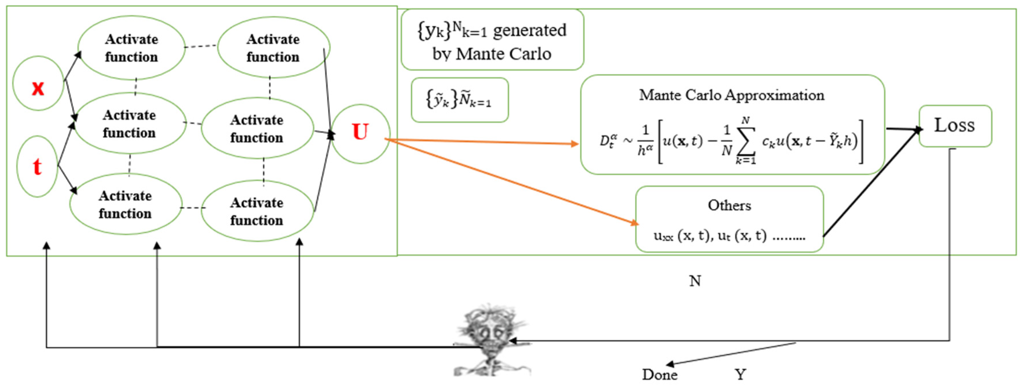
Figure 2.
Graphical illustration of PINN-CS overlaps with the exact solution of 2D space fractional PDE in example 3.1.
Figure 2.
Graphical illustration of PINN-CS overlaps with the exact solution of 2D space fractional PDE in example 3.1.
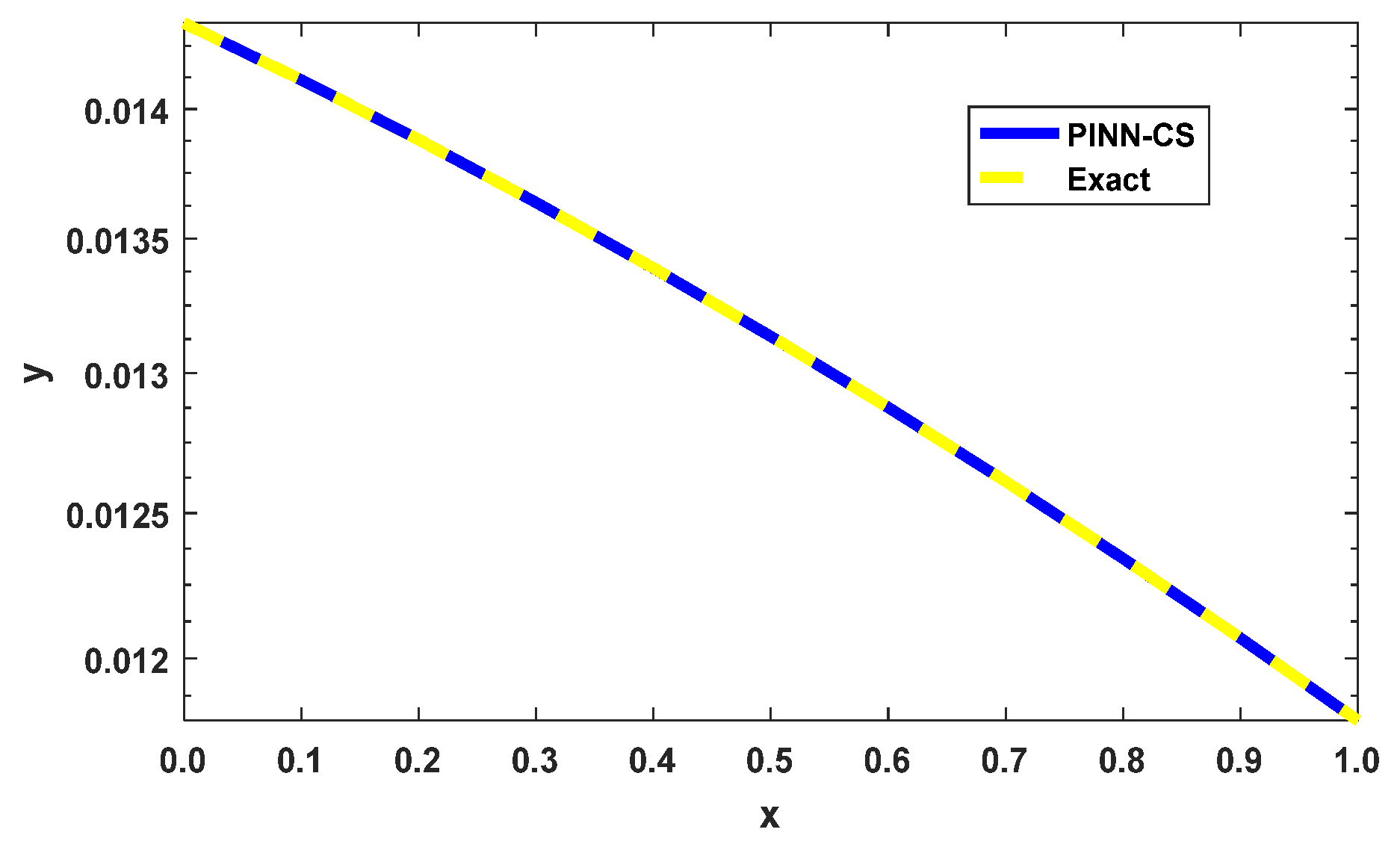
Figure 3.
Performance of PINN-CS overlaps with the exact solution of 2D time-space fractional diffusion equations for example 3.2.
Figure 3.
Performance of PINN-CS overlaps with the exact solution of 2D time-space fractional diffusion equations for example 3.2.
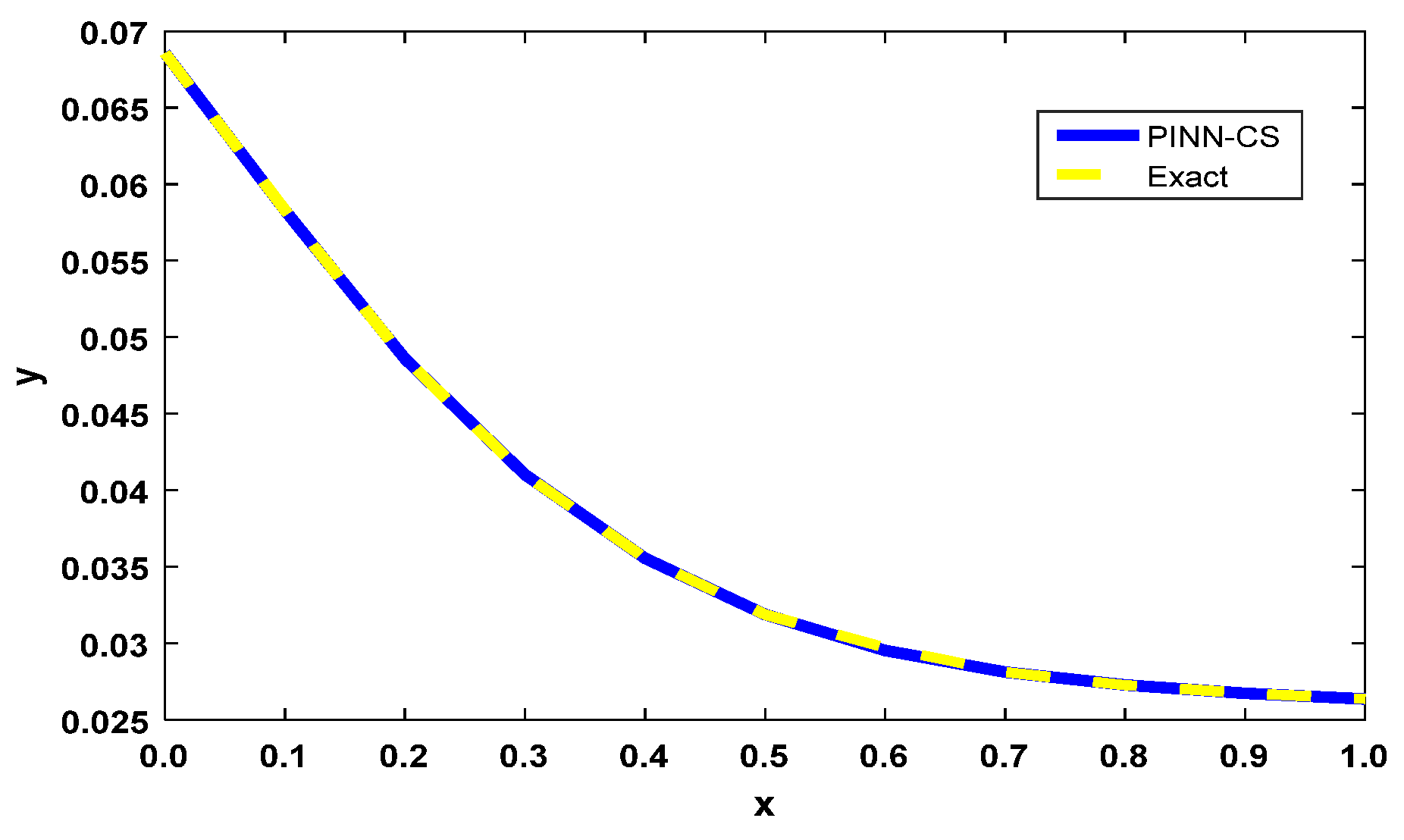
Figure 4.
Show the performance of the PINN-CS overlaps the exact solution of example 3.3.
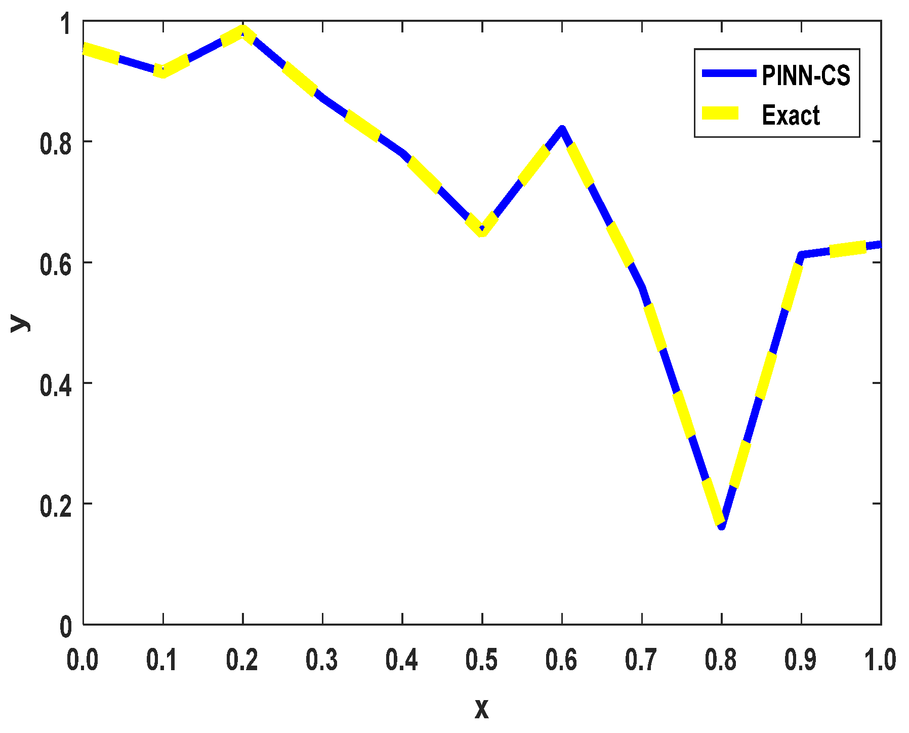
Figure 5.
Show the performance of the PINN-CS overlaps the exact solution, for example 3.4.
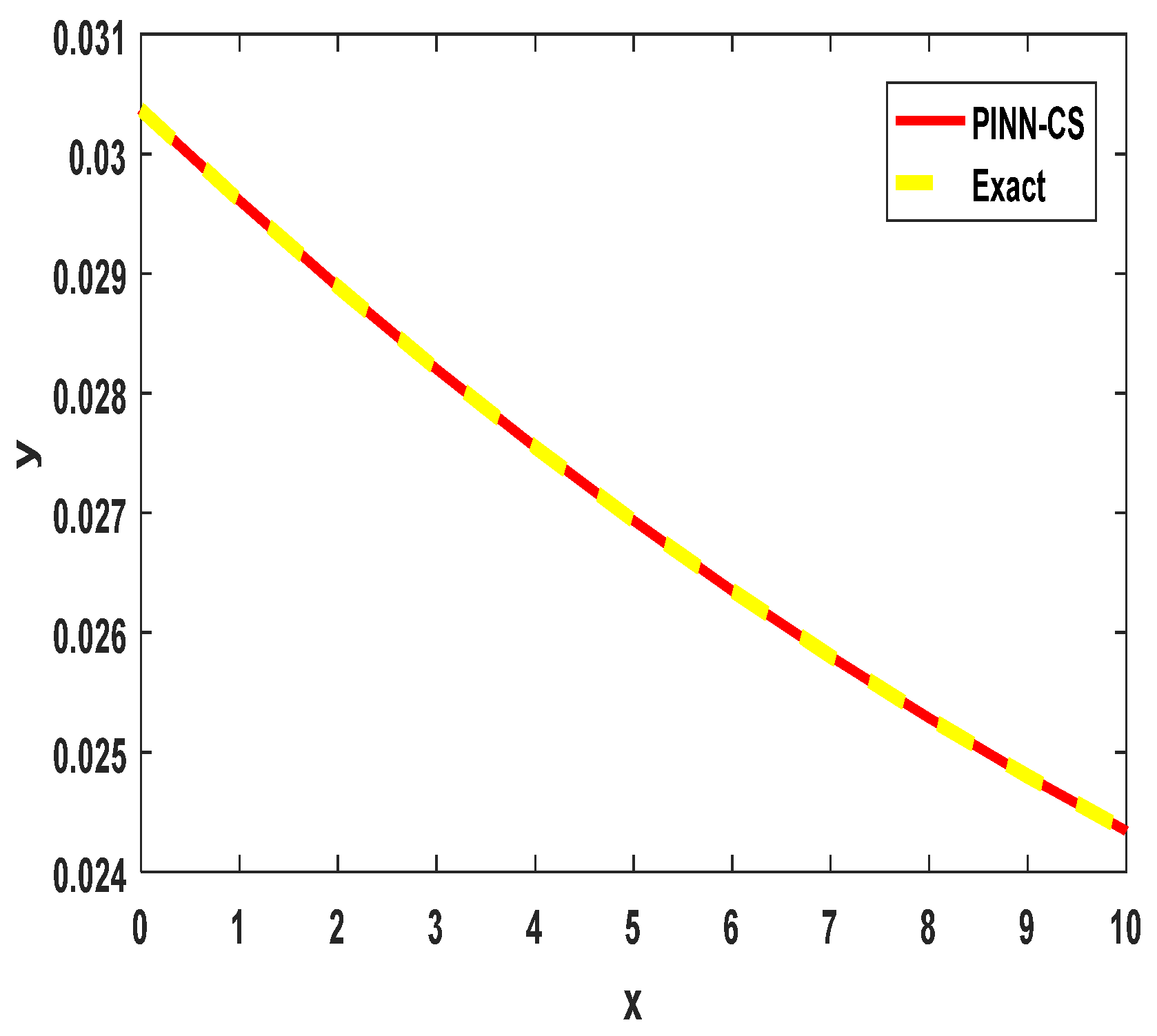
Figure 6.
Point-wise error distribution of 2D space fractional PDEs for example 3.1.
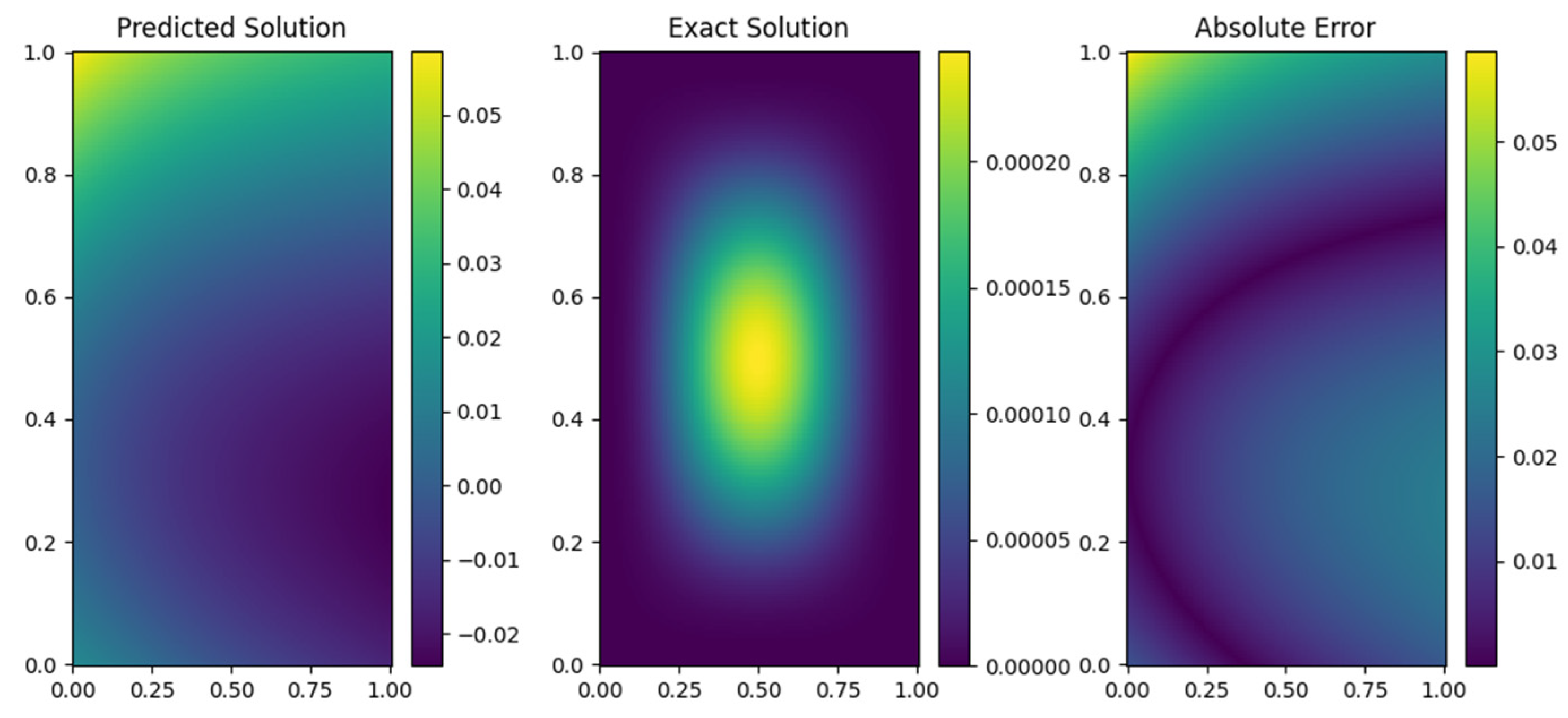
Figure 7.
Point-wise error distribution of 2D time-space fractional diffusion equations for example 3.2.
Figure 7.
Point-wise error distribution of 2D time-space fractional diffusion equations for example 3.2.
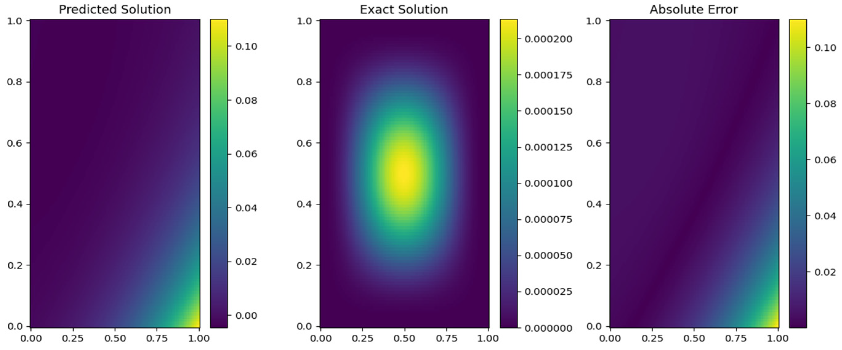
Figure 8.
Pointwise error distribution error of 3D time-space fractional Bloch-Torrey equations for example 3.3.
Figure 8.
Pointwise error distribution error of 3D time-space fractional Bloch-Torrey equations for example 3.3.
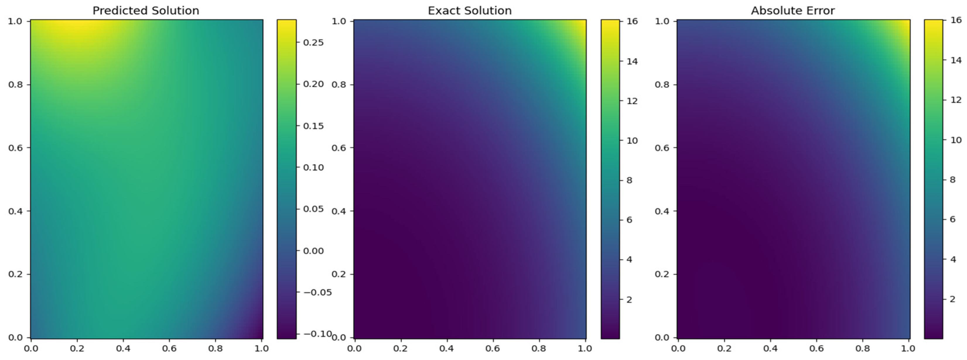
Figure 9.
Show the point wise error distribution of 3D Bloch Torrey equations for example 3.4.
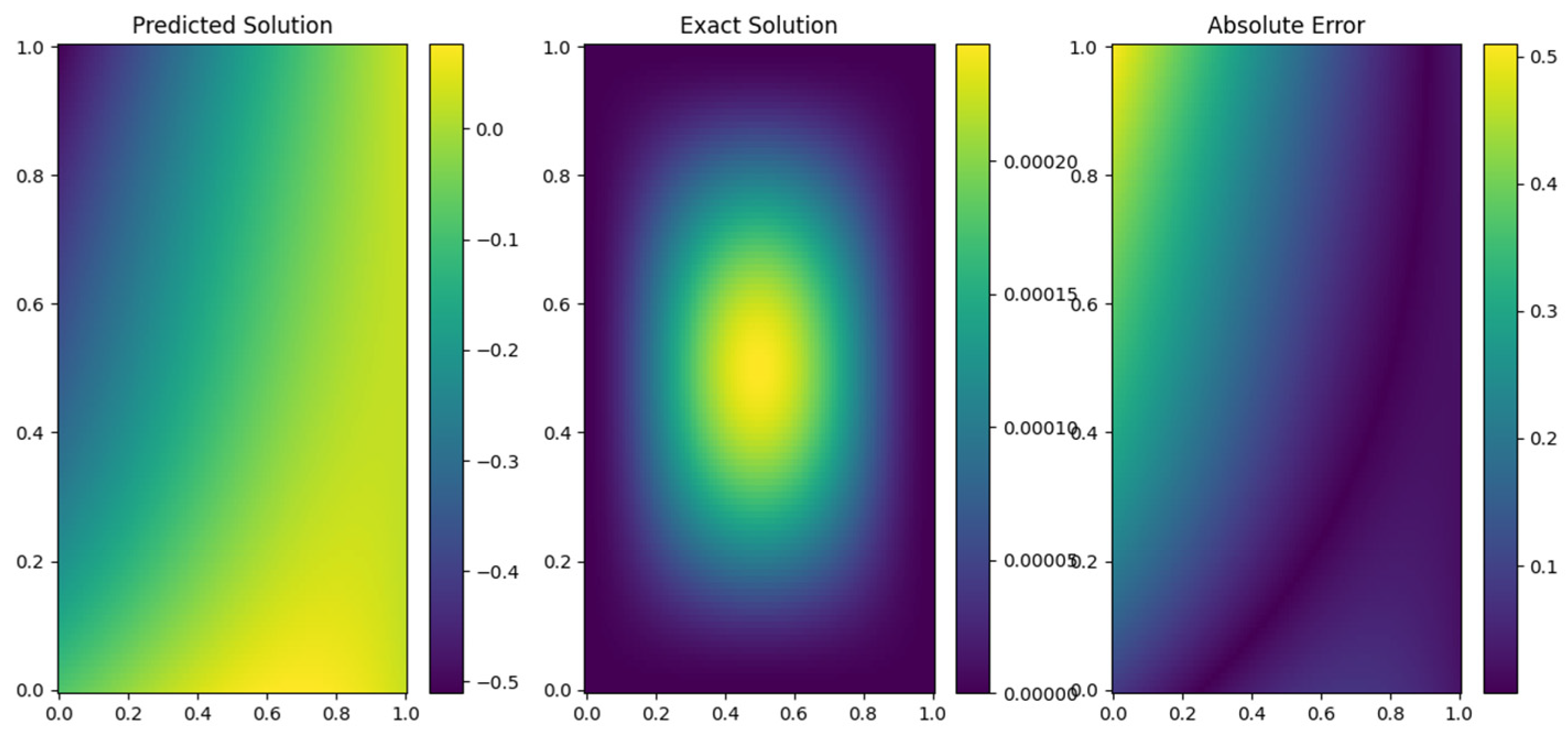
Figure 10.
Illustration of 3D solutions graph for example 3.1.
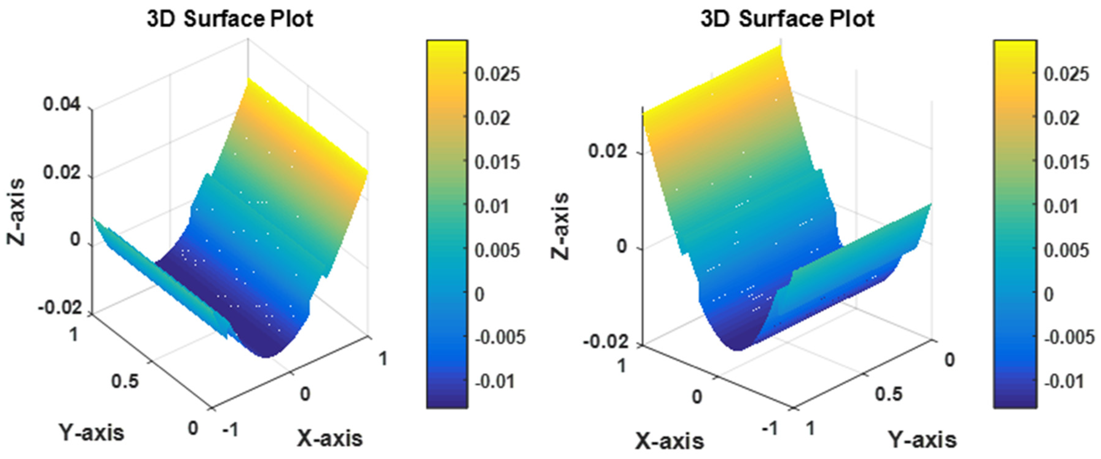
Figure 11.
Show the 3D graph for example 3.2.
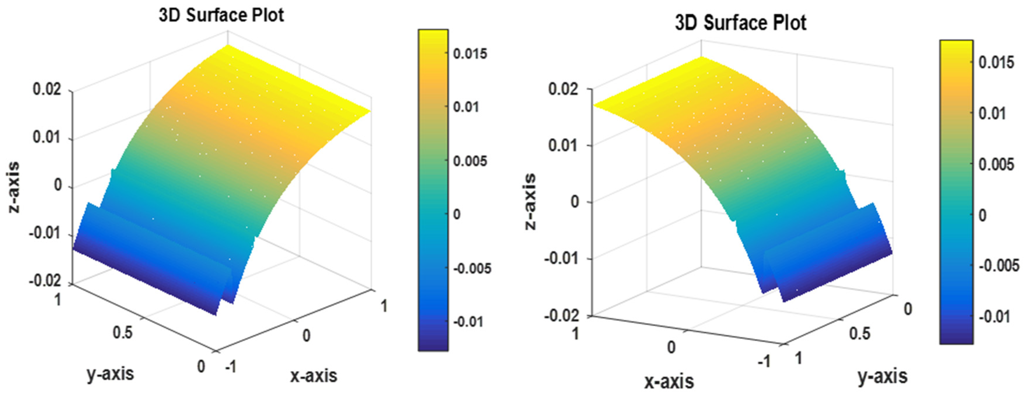
Figure 12.
Best fitness vs. generation of 2D space fractional PDE in example 3.1.
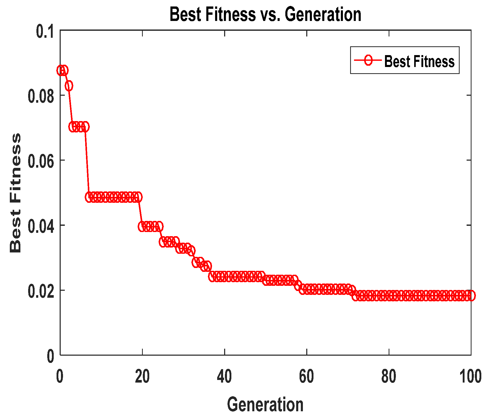
Figure 13.
Displays the optimal fitness versus generation for the 2D time-space fractional diffusion equations in example 3.2.
Figure 13.
Displays the optimal fitness versus generation for the 2D time-space fractional diffusion equations in example 3.2.
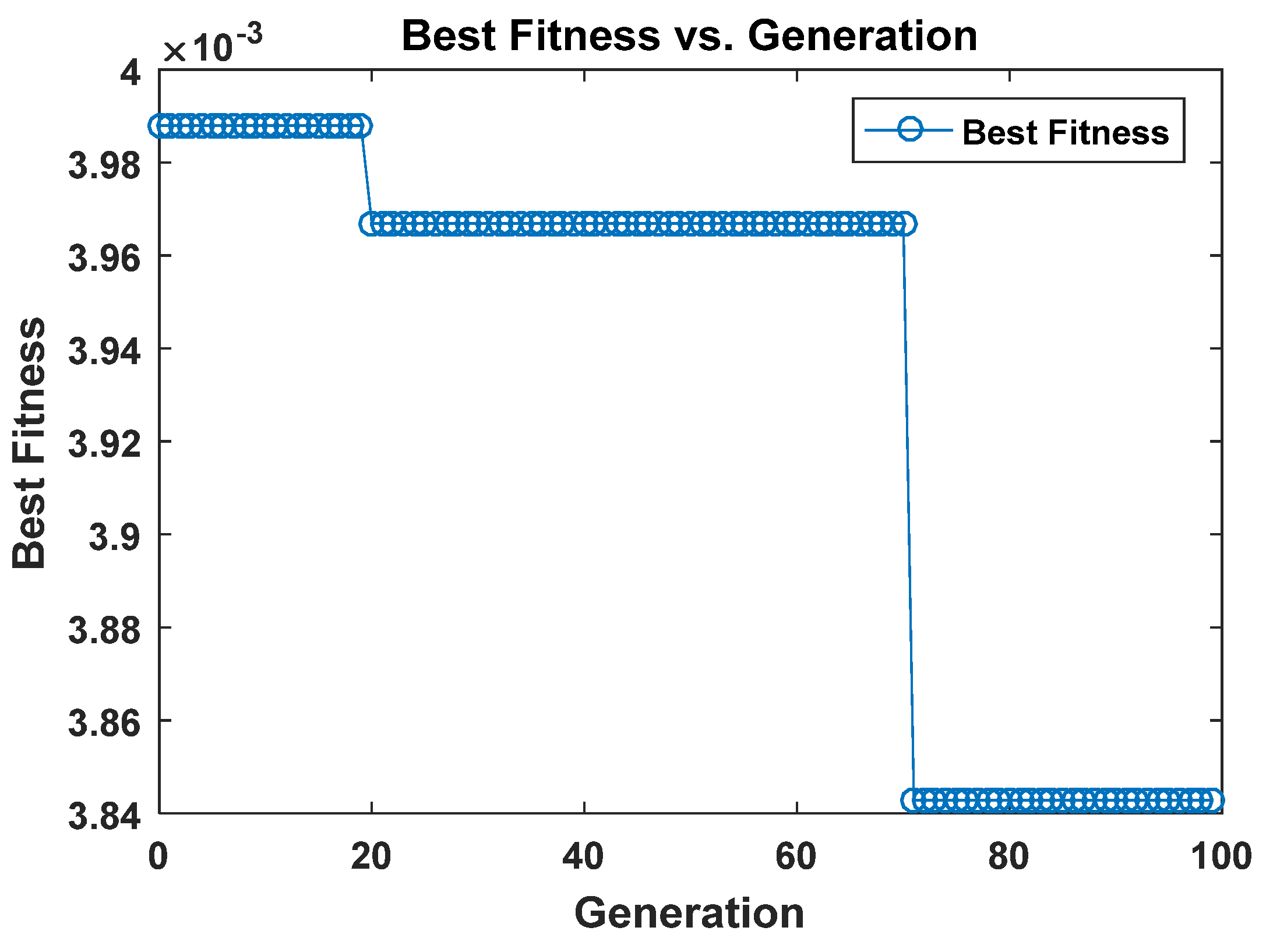
Figure 14.
Illustrates the optimal fitness versus generation for the 3D time fractional Bloch-Torrey equations in example 3.3.
Figure 14.
Illustrates the optimal fitness versus generation for the 3D time fractional Bloch-Torrey equations in example 3.3.
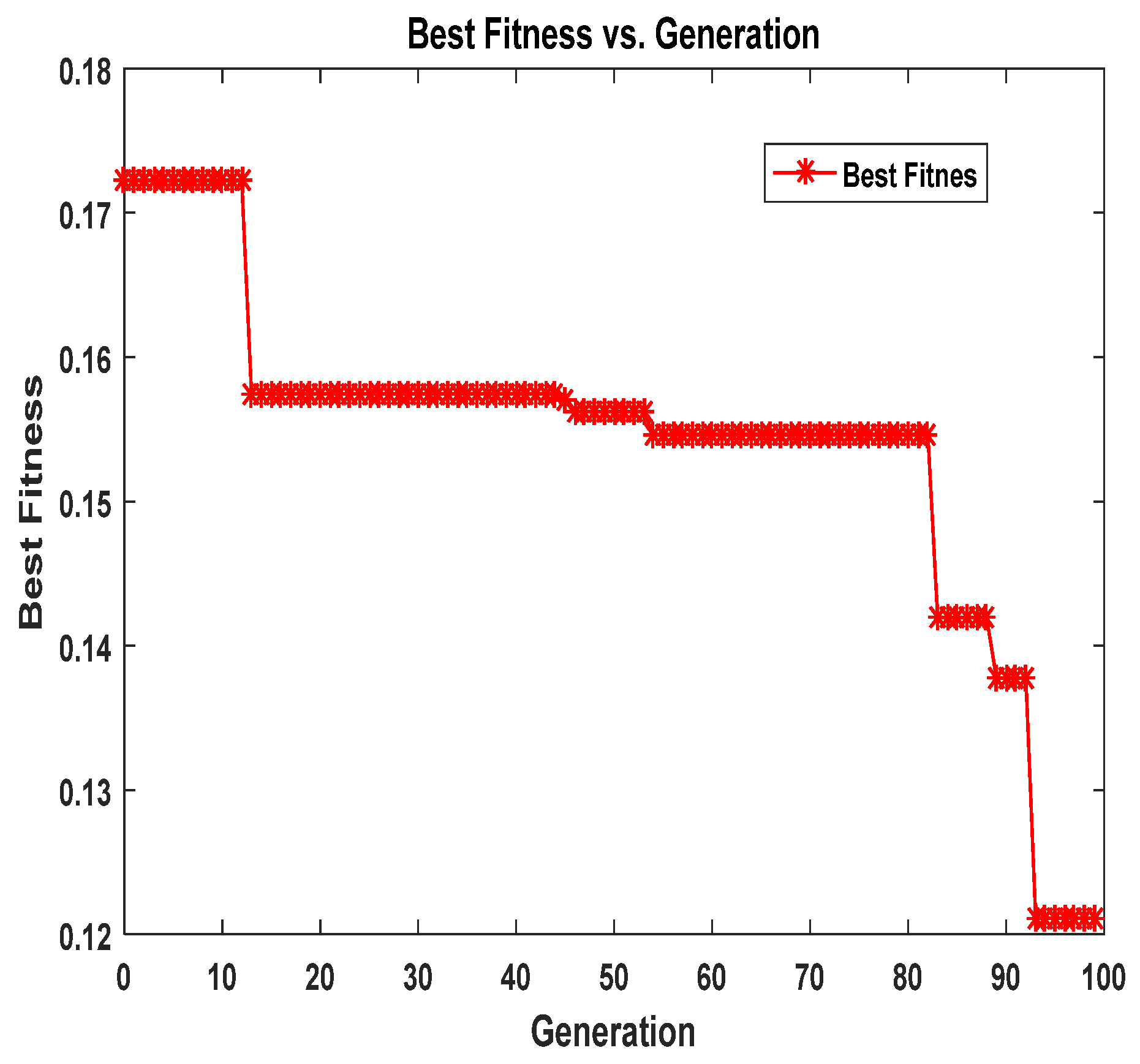
Figure 15.
Displays the optimal fitness against the generation for the 3D time fractional Bloch-Torrey equations in example 3.4.
Figure 15.
Displays the optimal fitness against the generation for the 3D time fractional Bloch-Torrey equations in example 3.4.
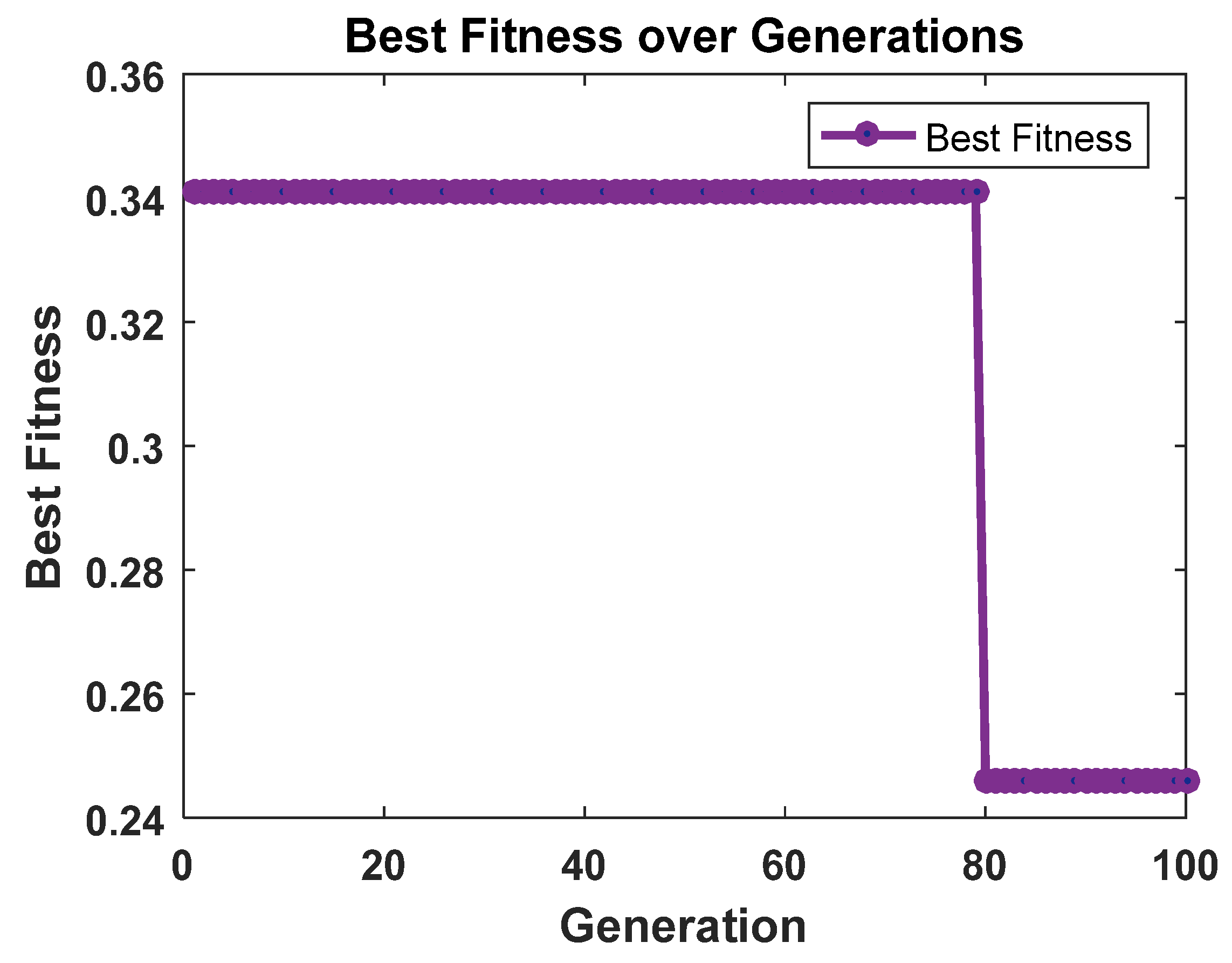
Figure 16.
Visual representation of the absolute errors in solving the 2D space fractional PDE in example 3.1.
Figure 16.
Visual representation of the absolute errors in solving the 2D space fractional PDE in example 3.1.
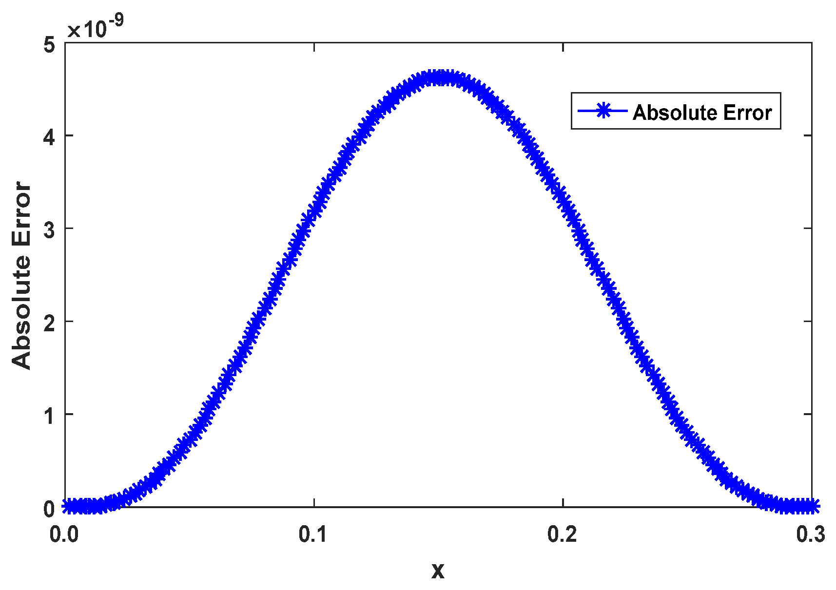
Figure 17.
Display the absolute errors for the 2D time-space fractional diffusion equations in example 3.2.
Figure 17.
Display the absolute errors for the 2D time-space fractional diffusion equations in example 3.2.
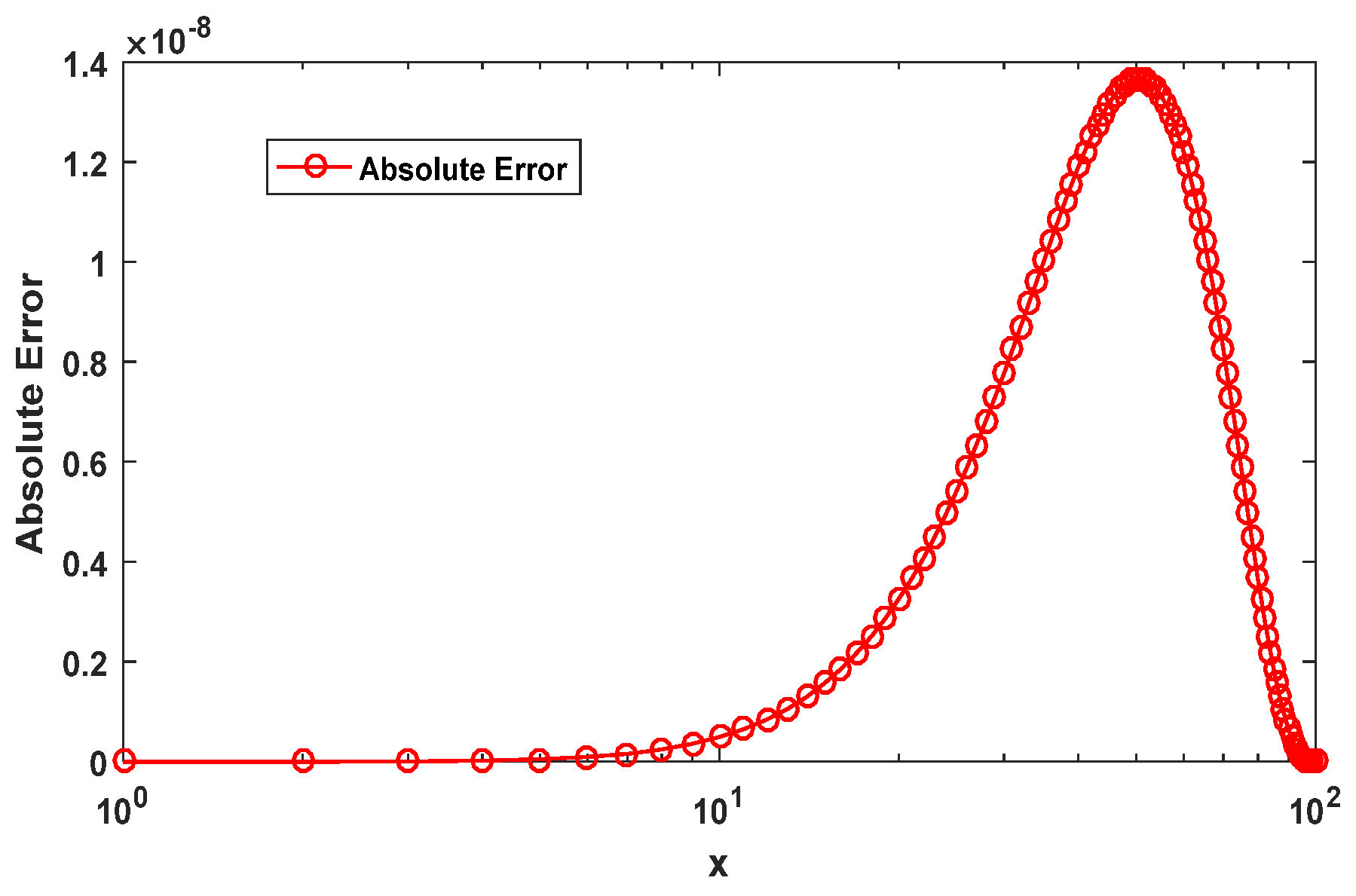
Figure 18.
Display the absolute error for the 3D time-space fractional Bloch-Torrey equations in example 3.3.
Figure 18.
Display the absolute error for the 3D time-space fractional Bloch-Torrey equations in example 3.3.
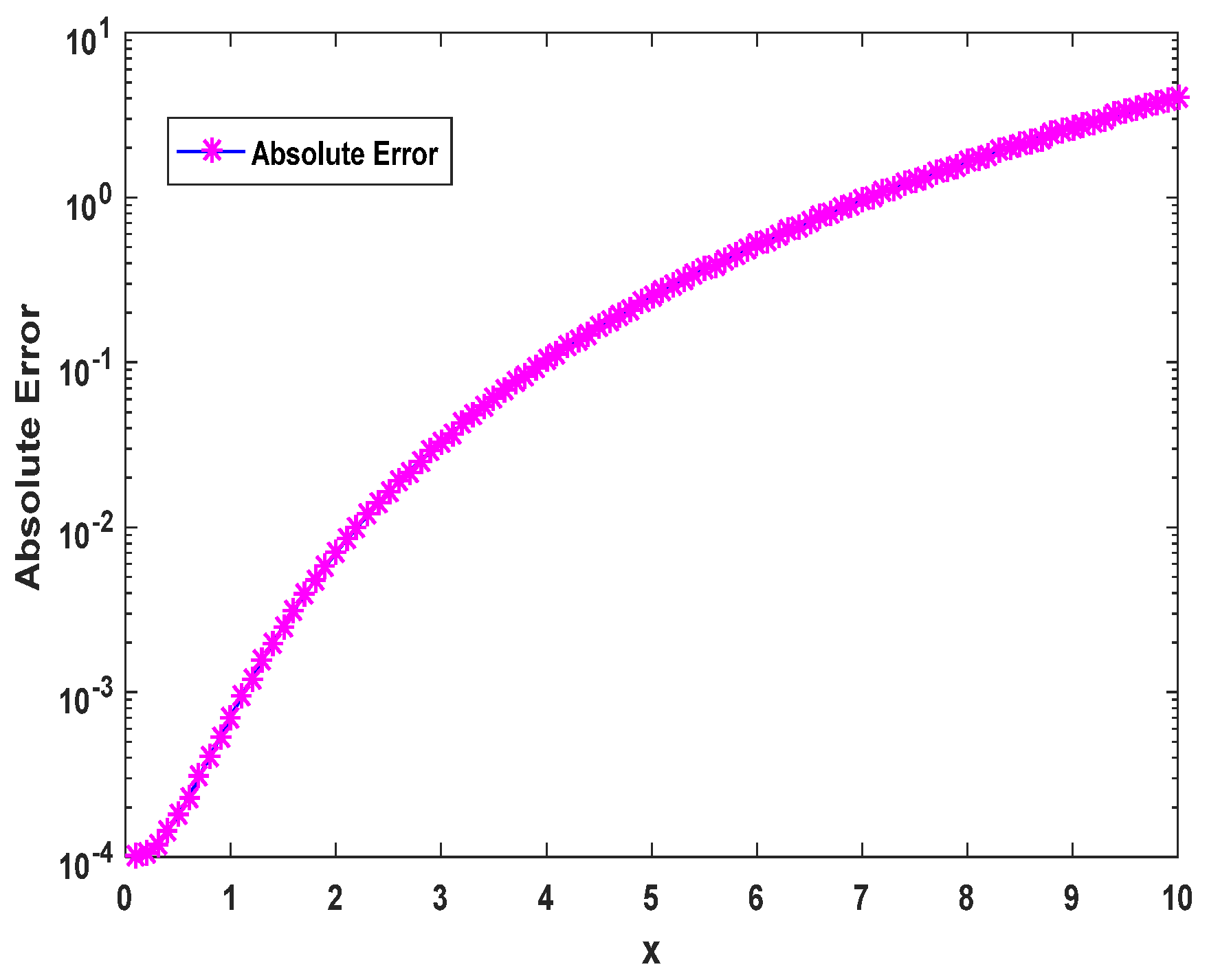
Figure 19.
Present the absolute error for the 3D time-space fractional Bloch-Torrey equations in example 3.4.
Figure 19.
Present the absolute error for the 3D time-space fractional Bloch-Torrey equations in example 3.4.
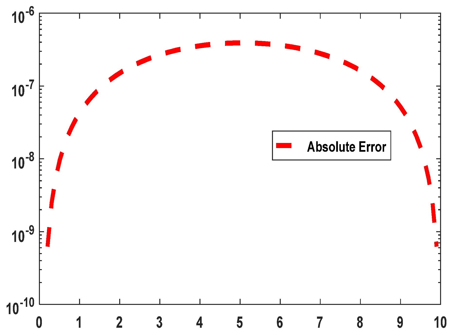

Table 1.
Parameter settings for example 3.1 (2D space fractional PDEs.).
| Parameter | Value |
|---|---|
| Approximate point | 150 |
| Hidden layers | 4 |
| Neurons | 5 |
| Activation function | tanh |
| Optimizer | Cuckoo Search Algorithm |
| Number of iterations | 1000 |
| 1.7 | |
| 1.5 |
Table 2.
We compare the performance of fPINN [29], Monte Carlo fPINN [31], and the PINN-CS technique on a disc with , and for example 3.1.
| N | FPINN | Mante Carlo PINN | PINN-CS |
|---|---|---|---|
| 8 | 3.73×10-01 | 2.91×10-01 | 3.88×10⁻¹¹ |
| 16 | 1.73×10-01 | 1.45×10-01 | 2.60×10⁻¹⁰ |
| 32 | 6.71×10-02 | 5.97×10-02 | 1.12×10-09 |
| 64 | 3.97×10-03 | 1.42×10-02 | 4.35×10-09 |
| 128 | 9.54×10-03 | 8.06×10-03 | 5.25×10⁻¹⁰ |
Table 3.
Show the parameter setting for examples 3.2 (2D time-space fractional diffusion).
| Parameter | Value |
|---|---|
| Approximate point | 100 |
| Hidden layers | 4 |
| Neurons | 5 |
| Activation function | tanh |
| Optimizer | Cuckoo Search Algorithm |
| Number of iterations | 1000 |
| 0.3 | |
| 1.7 |
Table 4.
Comparison of performance between fPINN [29], Mante Carlo PINN and PINN-CS method (2D time space fractional diffusion equation) on Ω1 for example 3.2, for α = 0.3, β = 1.7.
Table 4.
Comparison of performance between fPINN [29], Mante Carlo PINN and PINN-CS method (2D time space fractional diffusion equation) on Ω1 for example 3.2, for α = 0.3, β = 1.7.
| N | fPINN | Mante Carlo PINN | PINN-CS |
|---|---|---|---|
| -01 | -01 | -09 | |
| -02 | -02 | -08 | |
| -02 | -02 | -09 |
Table 5.
Show the parameter setting, for example 3.3 (3D time-space fractional Bloch-Torrey equation).
Table 5.
Show the parameter setting, for example 3.3 (3D time-space fractional Bloch-Torrey equation).
| Parameter | Value | Parameter | Value |
|---|---|---|---|
| Approximate point N | Neurons | 5 | |
| Hidden layer | Activation function | ||
| Optimizer | Cuckoo Search algorithm | Number of iterations | 1000 |
| α | β | 1.5 | |
| 0.5 |
Table 6.
Show the performance of the PINN-CS of the 3D time-space fractional Bloch-Torrey equations of example 3.3.
Table 6.
Show the performance of the PINN-CS of the 3D time-space fractional Bloch-Torrey equations of example 3.3.
| N | PINN-CS | Exact | Absolute Error |
|---|---|---|---|
| -04 | |||
| -04 | |||
| -04 | |||
| -04 | |||
| -04 | |||
| -04 | |||
| -04 | |||
| -04 | |||
| -04 | |||
| -04 | |||
| -04 |
Table 7.
Show the parameter setting for problem 3.4 of 3D time-space fractional Bloch-Torrey equations.
Table 7.
Show the parameter setting for problem 3.4 of 3D time-space fractional Bloch-Torrey equations.
| Parameter | Value | Parameter | Value |
|---|---|---|---|
| Approximate point N | Neurons | 5 | |
| Hidden layer | Activation function | ||
| Optimizer | Cuckoo Search algorithm | Number of iterations | 1000 |
| 012 | β | 1.8 | |
| ub | 0.5 |
Table 8.
Show the predicted solution of PINN-CS and the exact solution of 3D Bloch Torrey equations for example 3.4.
Table 8.
Show the predicted solution of PINN-CS and the exact solution of 3D Bloch Torrey equations for example 3.4.
| N | PINN-CS | Exact Solution | Absolute Error |
|---|---|---|---|
| -10 | |||
| -09 | |||
| -09 | |||
| -09 | |||
| -08 | |||
| -08 | |||
| -08 | |||
| -08 | |||
| -08 | |||
| -08 |
Disclaimer/Publisher’s Note: The statements, opinions and data contained in all publications are solely those of the individual author(s) and contributor(s) and not of MDPI and/or the editor(s). MDPI and/or the editor(s) disclaim responsibility for any injury to people or property resulting from any ideas, methods, instructions or products referred to in the content. |
© 2025 by the authors. Licensee MDPI, Basel, Switzerland. This article is an open access article distributed under the terms and conditions of the Creative Commons Attribution (CC BY) license (https://creativecommons.org/licenses/by/4.0/).
Copyright: This open access article is published under a Creative Commons CC BY 4.0 license, which permit the free download, distribution, and reuse, provided that the author and preprint are cited in any reuse.


