
Submitted:
02 July 2025
Posted:
02 July 2025
You are already at the latest version
Abstract
This paper investigates a controversial phenomenon: the supposed generation of thrust from a symmetric system consisting of two contra-rotating gyroscopes whose spin axes form equal and opposite polar angles with respect to the axis connecting their supports. An elementary mechanical model demonstrates that, for this configuration of gyroscopes, an internal moment arises within the system. This torque, although internally generated, is well known to play a significant role in satellite attitude control using control-moment gyroscopes (CMGs). The mechanical analysis considers the system of gyroscopes mounted on a platform or cart, which is supported at its front and rear ends. In this context, it was found that the resulting dynamic interaction causes unequal reaction forces at the support points, which do not obey the length-ratio rule predicted by static analysis. Such behavior can lead to a misinterpretation of a net external thrust, despite the system being closed and momentum-conserving.
Keywords:
Control Moment Gyroscope
; Reaction Force
; Thrust
; Inertial Propulsion
1. Introduction
Over the past century, humanity’s aspiration for interstellar travel has sparked considerable interest in alternatives to traditional rocket propulsion (e.g., [1,2]). In simple terms, even today, launching a relatively small spacecraft requires an enormous volume of rockets for propulsion—an inefficiency that demands a solution. At the turn of the twenty-first century, two major initiatives addressed this challenge: Project Greenglow at BAE Systems [3,4,5,6,7] and NASA’s Breakthrough Propulsion Physics program [8,9,10,11]. The findings of the latter were compiled into a comprehensive 740-page book [12].
Alternative propulsion methods have been classified into much more than twenty categories—including Hall thrusters, the Casimir effect, and the EM-Drive—[11,12], one of which is known as inertial propulsion. The concept of inertial propulsion dates back to the early 1930s in Italy and Russia and later gained attention in the United States with the controversial "Dean Drive" [13,14], which proposed that two contra-rotating masses could produce unidirectional motion. In the mid-1970s, Eric Laithwaite, Professor of Electrical Engineering at Imperial College London, demonstrated that a heavy gyroscope could be lifted with surprising ease [15,16,17]. Most historical efforts related to inertial propulsion have been documented in a comprehensive review [18], while a more recent study has shown that continuous propulsion cannot be expected from rotating mass particles alone [19]. However, previous studies have not thoroughly explored the potential of gyroscope-based inertial propulsion.
While BAE Systems and NASA have made their alternative propulsion projects publicly available, the same cannot be said for Boeing Co. (USA). In October 2014, senior engineer Mike Gamble received permission from The Boeing Company to publicly disclose information on their control moment gyroscope (CMG) research. This disclosure took place in August 2015 and provided historical insight into Boeing’s CMG work [20]. As he noted in his authorized presentation: “The work started back in the 1960s and continued into the 1990s. The presenter got involved with it in 1995 when he took over operations of the Guidance, Navigation, and Controls (GN&C) lab at the Boeing Kent (WA) Space Center. This lab and the building that housed it were badly damaged in the 2001 Seattle earthquake and later demolished.” [20].
At the same conference, the same author presented a second paper [21], from which Figure 1 is derived, with his kind permission. It illustrates the sawtooth-shaped input torquing rate waveform (referred to as "scissoring") used to generate a pulsed output force. He claimed that by applying torque rapidly in one direction and slowly in the other, a pulsed (average) output force is produced—similar in waveform to that observed in systems involving rotating masses.
Furthermore, between 2017 and 2020, a series of four conference papers documented the development and testing of several alternative prototypes [22,23,24,25]. Each prototype featured a wheeled cart equipped with a differential control moment gyroscope (CMG). In these designs, the pair of CMGs did not rotate continuously through a full circle but instead oscillated in a contra-rotating manner within the range of []. To the best of our understanding, the main conclusions are as follows:
- When the intended thrust is upward, the average reaction force at two of the four cart wheels is also directed upward, consistent with the behavior shown in Figure 1.
- When the intended thrust is horizontal, the oscillation of the eccentrics results in smooth, continuous rolling of the cart along the ground (video-recorded in [25]). This effect is attributed to frictional forces, similar to those involved in human locomotion.
The purpose of this paper is to provide a detailed explanation of the first observation above, which has led some authors to persistently suspect that Newton’s third law may be violated in the operation of control moment gyroscopes (CMGs).
Extensive research has been conducted on Control Moment Gyroscopes (CMGs), with much of the work completed up to 2015 compiled and organized in the book by Leve et al. [26]. Key lessons learned from the use of CMGs on the International Space Station (ISS) were reported in 2010 by three industrial partners, including The Boeing Company [27]. Around the same time, NASA and Boeing also reported on on-orbit propulsion systems and momentum management strategies for the ISS [28].
Scissored-pair control moment gyroscopes (also known as twin gyroscopes) have existed for over a century. Brennan’s monorail system [29] employed two counter-rotating flywheels with interlinked gimbals to achieve symmetric stabilization during left or right turns. Like any CMG array, a scissored pair generates attitude-control torque by exchanging angular momentum with the host body. During the Skylab era, the Astronaut Maneuvering Research Vehicle utilized scissored pairs for attitude control [30]. These configurations have also been investigated as gyrodampers for large space structures [31].
In robotic applications with single revolute joints, where torque is required along a single axis, the symmetry inherent in a scissored pair enables torque generation without producing significant reaction torques in the robot itself. Such systems are capable of rapidly reorienting a payload with reduced power requirements compared to maneuvering the entire spacecraft [32]. Subsequent studies on this concept were conducted by Brown and Peck [33,34].
A recent layman-friendly explanation of CMGs and their role aboard the International Space Station (ISS) has been presented by National Geographic [35]. It emphasizes that the change in orientation caused by gyroscopic axle motion is primarily powered by solar energy, thus eliminating the need for propellant consumption.
It is important to note that, despite changes in orientation, the satellite’s center of mass remains at a constant distance from the nearest planetary body and is therefore not directly propelled in the radial direction. However, by altering the satellite’s orientation, CMGs can indirectly influence its trajectory and position over time—particularly when combined with additional mechanisms that exploit orientation changes, such as gravity-gradient stabilization, solar sails, electrodynamic tethers, or auxiliary thrusters.
In the context of spacecraft propulsion, and in addition to the aforementioned methods, electrolysis propulsion [36] involves the use of electrical energy to dissociate water () into its constituent elements—hydrogen () and oxygen (). These gases can subsequently be employed as propellants in a thruster system. Unlike the previously discussed methods, which primarily alter orientation without affecting the spacecraft’s center of mass, electrolysis propulsion results in the expulsion of mass and can thus induce a shift in the spacecraft’s center of mass and produce net translational acceleration [37].
In addition to the aforementioned contributions, the team at the Georgia Institute of Technology (USA) has made significant advances in singularity avoidance and steering laws, nonlinear control techniques, fault-tolerant control, CMG array configurations and dynamics, as well as comprehensive reviews of CMG technologies [38,39,40,41,42]. Furthermore, researchers from the United Kingdom have contributed notably to the development of CMG systems, particularly in the context of small satellite platforms and advanced control strategies [43,44,45].
Beyond space applications, experimental terrestrial setups have also been developed, such as those aimed at stabilizing walking robots [46]. Early research explored the possibility that gyroscopes could generate net thrust [47], but later efforts focused on utilizing the angular momentum of flywheel gyroscopes for purposes such as vibration isolation in vehicles [48] and stabilization in two-wheeled self-balancing robots [49].
It is important to note that the mechanical analyses in the abovementioned literature are primarily limited to internal torque effects, with little or no discussion of the externally induced inertial forces. In contrast, the core focus of the present paper lies in the analysis of the net force generated by such systems.
As stated earlier, the objective of this paper is to offer a consistent explanation—grounded in Newtonian mechanics—for the observed reinforcement of one of the support reactions of a cart-mounted CMG. Obviously, if the same had been demonstrated for the entire cart, this would eliminate any remaining doubts about a CMG’s potential to produce inertial propulsion and induce motion of the system’s center of gravity.
2. Materials and Methods
2.1. General
We present a simplified setup of a dual gyroscope mounted on a cart, inspired by the excellent work (design, manufacturing, and assembly) of Mike Gamble and his partner Dr. Tom Valone on a tabletop version of a newly designed CMG (a simplified miniature of the old one destroyed in 2001 at Boeing’s premises), which was orally presented in a series of talks in International Conference on Future Energy (COFE) [21,22,23,24,25]. Nevertheless, the proposed setup has not been confirmed by them, which means that it may differ from the prototypes to an unknown extent, and thus the mechanical model is the author’s responsibility.
We consider a right-handed Cartesian coordinate system , originated at the centroid G of a wheeled cart, where y is the upward vertical axis. Let ABCD be the top view of a cart (on horizontal plane ), on which two contra-rotating gyroscopes are mounted (see, Figure 2). On the upper horizontal surface of the cart, we consider two parallel spindles (with axes and ) which contra-rotate in their corresponding cage, firmly connected to the cart. Perpendicularly to each of these two shafts, is pivoted the axle of the corresponding gyroscope, the first () at the left shaft and the second () at the right shaft . In other words, the illustrated symbols (L) and (R) refer to the left and right spinning wheel, respectively.
Although the system is primarily designed for testing vertical thrust, the cart is equipped with wheels to allow for horizontal thrust evaluation as well (toward z-direction), thereby enhancing generality. The cart supports rigid mounting plates (not shown) that carry the twin Control Moment Gyroscope (CMG) system, as illustrated in Figure 2:
- The propulsion system consists of two identical gyroscopes that undergo controlled rotation (forced precession) about parallel spindles, positioned at the same height above the horizontal ground. The ideal geometric axis of each spindle is fixed relative to the cart. As is customary, each spinning wheel is housed within a circular ring, with its spin axis mounted on a gimbal. These two frames are mutually perpendicular and behave as a rigid body with one degree of freedom (see the third bullet below for further details).
- Each gyroscope is spun by an electric motor (driver) mounted on the gimbal, maintaining a nearly constant spin rate, .
- The single degree of freedom for each gyroscope (illustrated in Figure 2b), along with the associated spindle rotation, is actuated by a servomotor. This torquer is applied at the intersection point between the circular ring and the gimbal.
- When the axes of the synchronized gyroscopes are coaligned, they share the same magnitude and direction of angular velocity (see, Figure 2a). Nevertheless, on the left gyrocope (L) the vector of angular momentum is directed from the pivot toward the spinning wheel, whereas on the right gyroscope (R) from the spinning wheel to the pivot .
2.2. Differential Torques
Next is the detailed mechanical analysis of differential torques. Note that the ends of the two spindles are pivoted to the cart, at a separation distance D in the x-direction. Quite schematically, Figure 3 illustrates the vertical plane on which the two gyroscopes rotate about the axes (spindles) oriented in the horizontal direction and passing through the points L (left) and R (right), which here are the same as the points and illustrated earlier in Figure 2. For the sake of easiness, we assume that the center of gravity G lies in the middle of the segment (LR) and, obviously, it always remains at the same position (actually it merely oscillates along the y axis). By construction, the gyroscopes perform rotations of 90 degrees, and thus for the polar angle we have .
When (horizontal axles), the spins of the gyroscopes are in the same x-direction, as shown by the blue-colored arrows in Figure 2a as well as in Figure 3a. In the general case, setting the symbols and to represent the unit vectors in the directions x and y, respectively, given magnitude of the angular momentum of the rotor, , for the arbitrary polar angle we have the following momenta for the left and the right gyroscopes:
and
Therefore, the total (resultant) angular momentum becomes (see also Figure 3b):
As a result, the application of Newton’s second law (in rotation) on the gyroscope results in
where is the angular velocity of the servomotor which controls the function .
Based on Newton’s third law, the internal torque applied from the gyroscopes to the cart will be the algebraically negative of that in Eq. (4), and thus
Therefore, the fully controlled motion of the dual gyroscopic system leads to an internal torque (given by Eq. (5)), which is entirely transmitted to the cart.
Considering Eq. (5), the well known formula:
and also the above definition , we eventually have:
Although the longitudinal vertical plane , which is located in the middle of the distance D, is a plane of symmetry (geometrically), due to the same chosen direction of the spin vectors, the total change of the total (resultant) angular momentum is a vector
which points in the negative direction of the horizontal x-axis, as shown in Figure 3b. This is also illustrated by the internal torque shown on the left side of Figure 3a, and is given by:
2.3. On the Modelling the Inertial Forces
In general, for the problem under consideration, inertial forces are distinguished in two sets, as follows:
- Due to rotating masses (Dean-drive term). This kind will be discussed below in current sub-section.
- Due to gyroscopic motion. This kind was covered above in sub-section 2.2.
The contra-rotating gyroscopes –accompanied with their corresponding driver motor– induce inertial forces, which can be easily determined by the kinematic restriction:
where r is the eccentricity of the rotating mass m.
Therefore, the total inertial force (from both gyroscopes, each of mass m), which is exerted as a supposed external force on the cart, will be:
Note that m is the concentrated mass of each gyroscope plus the corresponding driver motor, and r is the eccentricity of the center of mass of this rotating system. The factor 2 was set due to the contribution of two gyroscopes. Moreover, it is noted that the force components on the horizontal plane are cancelled due to the contra-rotation.
Since it is not clear how the angular velocity is controlled to vary, in this paper we shall adopt the following two models:
- Approximate Model: Constant angular velocity per phase: one high for rise and another low for reset.
- Exact Model: Variable angular velocity, which vanishes at the ends of the angular oscillation (), where the polar angle corresponds to the transition from `rise’ to `reset’.
2.4. Dynamic Equilibrium: Newton’s Laws
Let us consider the static equilibrium of the cart in which the external excitation force is the sum of the downward total dead weight () plus the vertical components of the two contra-rotating radial inertial forces toward the vertical y-direction:
At this point, we distinguish the abovementioned two cases, i.e. of piecewise-constant or variable angular velocity .
2.4.1. Approximate Model: Piecewise-Constant Angular Velocity
In this case, by virtue of Eq. (11) in conjunction with , Eq. (12) becomes:
where represents the speed of the servomotor and r is the eccentricity of each rotating mass. Then, the torque equilibrium by the front force () and the rear force () gives
while the force equilibrium in the vertical y-direction implies:
Solving the linear system of Eq.( 14) and Eq. (15), the analytical expressions for the two reaction forces become:
and
Splitting the excitation force in static and centripetal (Dean-drive) terms, and then substituting by the algebraic value of Eq. (4), the set of Eqs. () and () becomes:
and
Before going on, it is worthy to mention that usual contra-rotating inertial drives (called Dean drives) operate at constant angular velocities. Due to this fact, in this paper we have called the first term in Eqs. (18)-(19) as `Dean-drive term’, because it refers only to centripetal forces produced by the rotation of the out-of-balance concentrated mass .
- Both reaction (ground) forces at the front and rear ends of the cart are influenced by the inertial forces () as well as the gyroscopic term ().
- While in the Dean drive the excitation force is distributed proportionally to the lever lengths ( and ) as shown by the second terms inside the square brackets, the asymmetry due to the internal torque (directed to the negative of x-axis) –imposed by the operation of the dual gyroscopes– results in an equal differentiation of the reaction forces at front (with sign +) and rear (with sign -) supports. In other words, what is lost at the front support is gained at the rear support, and vice versa.
- When (i.e., axles beyond the horizontal level), if we isolate the out-of-balance mass (Dean drive term), it relieves both the front and rear reaction forces. Nevertheless, the additional gyroscopic term operates as follows: the front reaction force further decreases while the (previously decreased by the Dean-drive term) rear force now increases. The latter finding is in accordance with the experimental results reported by the creators of the prototypes [22,23,24,25], and thus the above discussion demystifies them.
- For given , the difference between the Dean drive effect and the gyroscopic effect, highly depends on the spin () and thus on the associated angular momentum .
2.4.2. Exact Model: Variable Angular Velocity
To meet the initial conditions where gyroscope’s frame must be at rest when arriving at the ends of the oscillation, a promising approach is to interpolate the polar angle between the endpoint values and using Hermite polynomials:
where is a parameter which refers to the portion of elapsed time t:
Therefore, the angular velocity is given as:
whereas its derivative is as follows:
One may easily verify that at the initial time () and final time () of the oscillation from to , Eq. (22) implies the desired stationary condition , and thus can be used for the purposes of this simulation.
Similar considerations may be assumed for the reset phase as well. Then, the initial state is , the final is , whereas the elapsed time is .
In the general case of variable angular velocity , the reaction forces become:
and
2.5. Operation
In the beginning of each cycle (period) at time , both axles ( and ) are simultaneously found at polar angle , and progressively move upwards until the position at time . In this upward phase, the mean average angular velocity is . To give priority to the rising up phase, the gyroscopes’ axles return to their initil position at smaller speed (i.e., ), which obviously is of negative sign (i.e., ). The procedure is schematically shown in Figure 4.
2.6. Impulse of Reaction Forces
2.6.1. Approximate Model
A close look at Eqs. (18)-(19)–in the Approximate Model–reveals that the sum of the two reaction forces is not affected by the gyroscopic terms, because they cancel one another; practically they compose a couple of equal and opposite forces which cancels . Therefore, the total vertical inertial force is influenced only by the measure of total centripetal force and the instantaneous polar angle .
Equations (18)-(19) are based on the assumption of constant angular velocity , otherwise its temporal velocity must be considered.
The total impulse of the reaction forces is given by:
where is the period. In more details, for each phase of motion, by integrating Eq. (18) and (19), we have:
I. Rise phase:
II. Reset phase:
In general, comparing Eq. (27) with Eq. (29), we obtain:
Also, comparing Eq. (28) with Eq. (30), we obtain:
Adding Eq. (31) and Eq. (32) by parts, we obtain:
which means that the impulse of both reaction forces in rise is equal and opposite to the impulse in reset. Therefore, as a general rule, whatever is probably gained in rise, is then lost in reset.
Obviously, if and , each term in Eqs. (27)-(30) vanishes, and therefore the total impulse of inertial forces within a period is zero. In contrast, if –for example– and , the impulse in each phase is different than zero, but again the total impulse per period is zero.
It is noted that the above discussion suffers from the fact that the assumed constant angular velocities do not satisfy the initial conditions of zero values at the initial (), the transitional () and the final position (), in each phase.
2.6.2. Variable Angular Velocity
To avoid the abovementioned complication regarding the definition of the function , we make the very reasonable assumption that the angular velocity exhibits even symmetry with respect to the polar angle , i.e.:
The above assumption is consistent with physical reality: the mechanical system must be at rest at (having just completed its downward motion), then its angular velocity gradually increases to a constant value during the upward motion, and eventually decreases to zero at (as it must reverse direction to initiate the next downward motion), and so on.
Mathematically, the above reasonable assumption (i.e., Eq. (34)) implies that the integrands and are odd functions (because ), and thus the time-integral of each reaction force (i.e., the impulse), due to both the Dean-drive and gyroscopic terms, in a period T vanishes.
Regarding the proposed closed-form analytical formula given by Eq. (20), it is easy to verify that it can also be written as follows:
Moreover, setting
it is trival to show that the function is also written as . Obviously, this is an even function in and also an even function in , because it fulfils the condition of Eq. (34). Therefore, the produced impulse over an entire period will vanish.
2.6.3. The Most General Case
The above choice of Hermite polynomials ensures an angular velocity which exhibits even symmetry with respect to the polar angle , i.e., satisfies Eq. (34). However, the aforementioned condition is not absolutely necessary, because any other piecewise continuous function leads to zero impulse of the reaction force due to the inertial forces.
Actually, regarding the gyroscopic term, since , the corresponding impulse within a period T is written as follows:
Therefore, the foregoing elementary analysis indicates that no net impulse is generated by the gyroscopic inertial forces. From a physical point of view, this is obvious considering the couple of equal and opposite reaction forces which withstands .
Let us now see what happens with the Dean-drive type of inertial forces, due to the rotating concentrated mass . To answer this question in a mathematical manner, the corresponding parts in Eq. (24) and Eq. (25) are written as follows:
and
Therefore, when integrating Eqs. (38) and (39) with respect to time t, the integral is canceled by the time derivative, and thus the total impulse becomes proportional to :
Since the initial and the final values are characterized by the condition , it is obvious that Eq. (40) dictates that the total impulse of the Dean-drive term at front support will vanish. Similar conclusion can be derived for the rear support as well (i.e., ).
Remark: Equation (40) shows that the impulse of the Dean-drive type inertial forces vanishes between any two states of vanishing angular velocity (). This case is met between and , between and , and so on.
3. Numerical Simulation
In this section we study two characteristic cases, as follows:
- Axle oscillation in the interval .
- Axle oscillation in the interval .
We apply (i) the Approximate model, which assumes constant angular velocities per phase (rise and reset), and (ii) the Exact model, which considers time varying angular velocity which fulfils the initial conditions (Hermite polyomials).
3.1. General Data
- Mass of gyroscope’s frame: g,
- Mass of gyroscope’s rotor: g,
- Mass of motor driver: g,
- Length of motor driver: mm,
- Rotor’s outer diameter: mm,
- Rotor’s inner diameter: mm,
- Rotor speed: RPM,
- Frame’s outer diameter: mm,
- Length of front end to centroid: m,
- Length of rear end to centroid: m (i.e., ).
- Time for rising phase: s.
- Time for reset phase: s.
3.2. Elementary Calculations
Based on the abovementioned data, the total oscillating mass (gyroscope plus motor driver) is:
The rotational inertia of gyroscope’s rotor is:
The angular momentum of gyroscope’s rotor is:
Regarding the eccentricity r which is involved in Eq. (18) and (19), the former is produced by the frame of mass at radius and the (assumed cylindrical) motor of mass and length . Due to the radius of the frame at which the motor is attached, the center of mass of the aforementioned motor is eventually at radius:
Therefore, applying the well-known rule for the center of mass of the system “gyro + motor”, the latter will give an eccentricity equal to:
while the rotating eccentric mass is
Therefore, the useful magnitude is:
Alternatively, the same result could be obtained when considering only the rotating eccentric mass of which is at distance , so that (i.e., the same as Eq. (47)).
Remark: While the data employed in this work are adapted from a previously reported prototype study [22,23,24,25], which involved a sophisticated design and integration process, it is important to underscore that the specific numerical values presented in Eqs. (41)–(43) are not critical to the overall conclusions of this paper. That is, the oscillating mass m has been chosen to be consistent with the associated angular momentum of the gyroscope’s rotor; however, any other compatible pair () would serve equally well.
3.3. Numerical Implementation of the Approximate Model
To derive numerical results using Eq. (18) and (19) for the piecewise-constant model, a computer program was developed according to the following algorithm:
- Split the rising interval (100 ms) into 100 equal segments, thus using a time step equal .
- At the end of the i-th time step calculate the current time instant by .
- Find the current polar angle by .
- Find the inertial force of Dean drive by .
- Find the differential gyroscopic torque by .
- Find the total vertical reaction force of the cart by .
- Find the vertical reaction force at the rear support by .
- Find the vertical reaction force at the front support by .
- Continue with the reset phase of the first cycle, in which is replaced by , the updated initial polar angle is and the final , while the new interval is divided into 600 equal time steps.
The weak point of this algorithm is the abrupt change of the angular velocity from to , within the first cycle. Keeping the time scale invariable as that in Figure 5 (), the value depends on the angle interval , so that:
whereas
Clearly, in the rise phase (within s) the driver motor rotates from to . Furthermore, in the reset phase (within s) the driver motor rotates in the opposite direction, from to , and thus returns to its initial position. Then, the next cycle is repeated, and so on.
Choosing () in conjunction with a total period of 0.7 s (), Eq. (48) leads to rad/s, whereas Eq. (49) results in rad/s, respectively, when the piecewise-constant model (Sect. 2.4.1) is applied.
Note: To avoid confusion due to the small magnitude of the inertial forces, in the next diagrams the dead-weight and the associated reaction forces are not included. In other words, the plotted reaction forces are only due to the inertial effect. Obviously, the total reaction forces is the superposition of the static and the inertial terms.
3.4. Servo Oscillation for
Applying the Approximate and the Hermite-polynomials (Exact) model, the corresponding calculated variation of the polar angle is illustrated in Figure 5. One may observe the close matching between the two models, as well as the fact that actually we have .
Moreover, for both models the calculated angular velocity for an entire period of s is illustrated in Figure 6. One may observe that the abovementioned constant angular velocities, i.e., rad/s and rad/s, are also the average values of the corresponding parts (rise, reset) when the Hermite-polynomials based model (Sect. 2.4.2) is applied.
Furthermore, for both models, the variation of the internal torque is illustrated in Figure 7. One may observe that the Approximate model cannot accurately simulate the initial (zero) angular velocity, but in general, is in good accordance with the Hermite model.
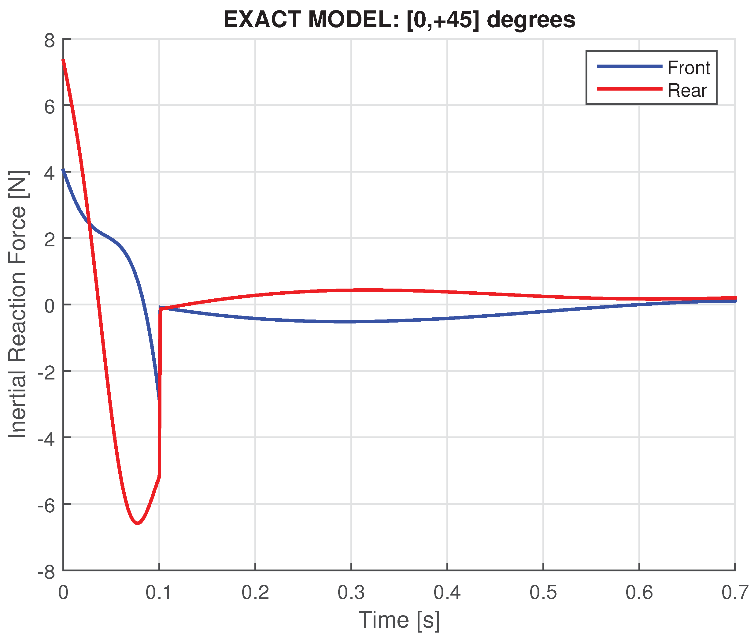
Based on the abovementioned internal torque and Dean-drive inertial term, Figure 8 presents the two computed vertical components (front, rear) of the inertial force using the Approximate model, while Figure 9 shows the corresponding results obtained from the Hermite model. In general, negative values indicate a downward support force acting on the cart, suggesting that the cart tends to lift. In contrast, positive values correspond to an upward support force, implying a tendency for the cart to move downward. Despite differences between the two models, the front support consistently exhibits smaller force magnitudes, thus giving the impression that it is less loaded.
3.5. Servo Oscillation for
Keeping the same durations, i.e., and , for both models, the same results with those of Sect. 3.4 are illustrated in Figure 10, Figure 11, Figure 12, Figure 13 and Figure 14. Since the duration of the rise phase remains the same for a halved angle, the average angular velocity and the internal torque are reduced by half. At the end, it can be observed that the rear support exhibits more negative values with larger absolute magnitudes, which gives the impression that the front support’s magnitude increases, while that of the rear support decreases.
4. Discussion
First, when the cart is stationary, the front and rear static reaction forces are distributed in proportion to the respective lever arm lengths between the supports and the center of gravity. Second, when a pair of contra-rotating masses is activated, the resulting first component of the inertial force—resembling that of a Dean drive—is also distributed between the front and rear supports according to the same lever-arm-based proportionality as the static case. Third, when these contra-rotating masses additionally undergo gyroscopic motion, a second component of the inertial force is generated. This force component is symmetrically shared between the front and rear supports such that any reduction in force at one support corresponds to an equal increase at the other.
Using two alternative models—one approximate and the other fully compliant with the initial conditions—this study has demonstrated that the generation of internal gyroscopic torque leads to equal-magnitude variations in the support forces (i.e., a couple of equal and opposite forces). It was found that the apparent ‘weight loss’ highly depends on the interval of axles’ oscillation. Specifically, when , the front support, which has the longer lever arm, experiences a local reduction in load, while the rear support correspondingly bears an increased load, locally. In contrast, when , the situation is reversed.
Having established the behavior of the maximum force values, it is important to emphasize that, over a full cycle, the time integral of the force at each support vanishes. Consequently, since the net impulse is zero, no net thrust is generated by this device.
Regarding the previously reported net thrust (cf. Figure 1), it should also be noted that in any experimental realization of the reported setup—or a similar configuration—the static (dead-weight) component at each support must be carefully subtracted. For example, if the subtracted value at the front support is even slightly underestimated, the measured force will not only appear reduced, but its time integral will deviate from zero. This may falsely indicate the presence of a net thrust.
It should be emphasized that there was no intention to undermine the value of prior scientific and technical contributions, as the objective was pursued in good faith. Comparable efforts in the area of inertial propulsion have been undertaken in various countries, as discussed in the following paragraphs.
In a previous study regarding inertial propulsion [18], it was reported that efforts to extend the distance traveled through mechanical means date back to ancient times, notably during the Olympic Games. More structured attempts began in Europe during the 1930s and later continued in the United States in the early 1950s [18]. The so-called Dean drive refers to a system composed of two contra-rotating masses that generate an oscillatory unidirectional force, which is proportional to the square of the angular velocity () [13,14]. Although it has been claimed that such devices are capable of producing thrust and thereby propelling a vehicle, detailed analyses—including those in Ref. [18]—demonstrate that any observed movement is attributable solely to the initial velocity of the rotating masses, rather than sustained propulsion. In simple words, the operation of the contra-rotating masses mimic a spring-mass system on the ground. Considering the friction between ground surface and an inertial device, the motion is possible [18], as was also demonstrated in [25]. However, the major problem is that even if an initial motion of the cart in the vertical direction becomes possible, when the cart reaches its upper point there is no more support to produce a second cycle, and so on [19].
Gyroscopes, on the other hand, continue to attract interest among proponents of inertial propulsion. Since the 1960s, both industrial and academic research groups have reported anomalous reaction forces during gyroscopic experiments, which have been interpreted by some as evidence of thrust generation or loss of weight [20,21,22,23,24,25,47]. These findings appear to contradict well-established physical laws. The analysis of such systems is more intricate than that of the Dean drive, primarily because the configuration of gyroscopic setups evolves over time. This complexity arises from the continuously changing orientation of the gyroscopes’ axes, which leads to corresponding variations in the angular momentum of the overall mechanical system. In contrast to the Dean-drive motion (proportional to ), the inertial force in contra-rotating gyroscopes is proportional to the product of two angular velocities (). The former () is due to the oscillation of gyro’s axle, while the latter () is the spin. Since the spin does not affect the bending strength of gyro’s axle even it takes a very high value, it is deduced that gyroscopes may develop higher inertial forces than those of the rotating masses (class of Dean drive devices).
A typical control moment gyroscope (CMG) system consists of an array of four gyroscopes [26]. Nevertheless, without loss of generality, and for the sake of simplicity, the ability to generate internal torque is illustrated here using only two gyroscopes. To elaborate, consider a satellite in orbit. While at rest—for example, during sleep—an astronaut exerts no torque on the spacecraft. However, internal torque can later be applied through hand movements or, equivalently, by actuating a mechanism that alters the relative orientation (e.g., the included angle) between the axes of two spinning gyroscopes, such as those considered in the present study. In such cases, Newton’s third law dictates that the internal torque generated is proportional to the angular velocity of reorientation, resulting in a change in the satellite’s orientation—i.e., its attitude—without affecting its translational motion. That is, the center of mass of the satellite remains fixed along its orbital path, while only its rotational state is altered.
When this principle is translated to a terrestrial setup (as is the case of present paper), the internal torque produced—such as through forced gyroscopic precession—must be counterbalanced by a couple of ground reaction forces, which have a zero sum. Therefore, the nonzero reaction forces are due to two separate reasons: First the distribution of the dead weight . Second, the reaction forces due to the ocillating masses in the interval ].
As a result, if one measures only the reaction forces at select points—particularly those that increase and even during a short time interval—this may create the illusion of a net propulsive force. However, such an effect does not violate Newtonian mechanics, as it merely reflects an internal redistribution of forces within a statically constrained system, not true propulsion.
A relevant interesting phenomenon of supposed weight loss was demonstrated in Professor Laithwaite’s 1974 lectures at University College London. In this experiment, a precessing gyroscope was mounted on an L-shaped aluminum stand positioned at the edge of a table. When the not spinning gyroscope was horizontally locked, its weight produced a torque that caused the stand to topple. In contrast, when the gyroscope was spinning at precession, no such overturn occurred (see approximately the 28-minute mark in the video [51], where Professor Laithwaite appears to demonstrate that a gyroscope undergoing forced precession exhibits a reduction in apparent weight).
5. Conclusions
A couple of oscillating control moment gyroscopes (CMG) is capable of producing an internal torque, which is very useful in attitude control. When the CMG is mounted on a terrestrial vehicle, the internal torque is counterbalanced by a couple of equal and opposite reaction forces, of zero sum. In addition to the gyroscopic forces which are induced due to the change of angular momentum, the oscillation also causes centripetal and tangential inertial forces which eventually are transmitted to the ground. Overall, the impulse of each reaction force within an entire period vanishes.
Funding
This research received no external funding.
Data Availability Statement
Data and software are available upon request.
Conflicts of Interest
The authors declare no conflicts of interest.
References
- Robertson, G.A.; Murad, P.A.; Davis, E. New frontiers in space propulsion sciences. Energy Convers. Manag. 2008, 49, 436–452. [CrossRef]
- Robertson, G.A.; Webb, D.W. The death of rocket science in the 21st century. Phys. Procedia 2011, 20, 319–330. [CrossRef]
- Allen, J.E. Quest for a novel force: A possible revolution in aerospace. Prog. Aerosp. Sci. 2003, 39, 1–60. [CrossRef]
- Meek, J. Bae’s Anti-Gravity Research Braves X-Files Ridicule. The Guardian, Mon 27 Mar 2000. Available online: https://www.theguardian.com/science/2000/mar/27/uknews (accessed on 22 June 2025).
- Anonymous. Project Greenglow and the Battle with Gravity. News, 23 March 2016. Available online: https://www.bbc.com/news/magazine-35861334 (accessed on 22 June 2025).
- Interview from Ron Evans. Available online: https://www.youtube.com/watch?v=BwI7Ij-5cMA&ab_channel=TimVentura (accessed on 22 June 2025).
- Wilson, J. Science Does the Impossible: February 2003 Cover Story. Popular Mechanics, Volume 180, No. 2. Available online: https://books.google.gr/books?id=UtMDAAAAMBAJ&printsec=frontcover&source=gbs_ge_summary_r&cad=0#v=onepage&q&f=false (accessed on 22 June 2025).
- Millis, M.G. Breakthrough Propulsion Physics Research Program. AIP Conf. Proc. 1997, 387, 1297–1302. [CrossRef]
- Millis, M.G. NASA breakthrough propulsion physics program. Acta Astronaut. 1999, 44, 175–182. [CrossRef]
- Millis, M.G. Assessing potential propulsion breakthroughs. Annu. N. Y. Acad. Sci. 2005, 1065, 441–461. [CrossRef]
- Millis, M.G. Progress in revolutionary propulsion physics, Paper IAC-10-C4.8.7. In Proceedings of the 61st International As-tronautical Congress, Prague, Czech Republic, 27 September–1 October 2010.
- Millis, M.G.; Davis, E.W. Frontiers of Propulsion Science; American Institute of Aeronautics and Astronautics Inc.: Reston, VA, USA, 2009.
- Dean, N.L. System for Converting Rotary Motion into Unidirectional Motion. U.S. Patent 2,886,976, 19 May 1959.
- Dean, N.L. Variable Oscillator System. U.S. Patent 3,182,517, 11 May 1965.
- Laithwaite, E.R. Propulsion Without Wheels, 2nd ed.; English Universities Press: London, UK, 1970.
- Wikipedia. Available online: https://en.wikipedia.org/wiki/Eric_Laithwaite (accessed on 23 January 2024).
- Laithwaite, E.R. The Engineer through the Looking Glass|The Royal Institution: Science Lives Here. Available online: https://www.rigb.org/explore-science/explore/video/engineer-through-looking-glass-looking-glass-house-1974 (accessed on 7 January 2024).
- Provatidis, C.G. Inertial Propulsion Devices: A Review. Eng 2024, 5(2), 851-880. [CrossRef]
- Provatidis, C.G. On the incapability of inertial forces as a means of repeated self-propulsion of an object in a vacuum. Proceedings of the European Academy of Sciences and Arts 2025, 4. [CrossRef]
- Gamble, M. History of Boeing control moment gyros (CMG). Presentation in Seventh International Conference On Future Energy (COFE7), July 30 – August 1, 2015, Embassy Suites, Albuquerque New Mexico (Boeing 15-00051-EOT).
- Gamble, M. Linear propulsion. Presentation in Seventh International Conference On Future Energy (COFE7), July 30 – August 1, 2015, Embassy Suites, Albuquerque New Mexico.
- M. Gamble, Dual CMG Gyroscopic Operation, COFE9, 30 July 2017.
- M. Gamble; T. Valone, Differential CMG (Part II), COFE10, 10 August 2018.
- M. Gamble; T. Valone, "Control Moment Gyro Experiment (Part III), COFE11, 9-10 August 2019, Albuquerque, NM.
- M. Gamble; T. Valone, Differential CMG (Part IV), COFE12, 14 August 2020. Online: https://www.youtube.com/watch?v=n1CH9_0Fs0E&ab_channel=ThomasValone (from 3:56:00 until 4:41:00).
- Leve F.A., Hamilton B.J. and Peck M.A. (2015) Spacecraft Momentum Control Systems. Springer, Cham.
- Gurrisi C., Seidel R., Dickerson S., Didziulis S., Frantz P., and Ferguson K. (2010) Space Station Control Moment Gyroscope Lessons Learned, Proceedings of the 40th Aerospace Mechanisms Symposium, NASA Kennedy Space Center, May 12-14, 2010, 161-175.
- Russell, S.P., Spencer, V., Metrocavage, K., Swanson, R.A., and Kamath, U.P. (2009) On-Orbit Propulsion and Methods of Momentum Management for the International Space Station, Proceedings 45th AIAA/ASME/SAE/ASEE Joint Propulsion Conference & Exhibit, 2 - 5 August 2009, Denver, Colorado, AIAA 2009-4899 (6 pages). [CrossRef]
- Brennan, L., Means for Imparting Stability to Unstable Bodies, US Patent 796893, 1905.
- Murtagh, T.B., Whitsett, C.E., Goodwin, M.A., "Automatic Control of the Skylab Astronaut Maneuvering Research Vehicle," Journal of Spacecraft and Rockets, Vol. 11, No. 5, 1974, pp. 321-326. [CrossRef]
- Aubrun, J.N., and Margulies, G., "Gyrodampers for Large Space Structures," NASA, 159171, 1979. Download from: https://ntrs.nasa.gov/citations/19800019916.
- M. D. Carpenter and M. A. Peck, "Dynamics of a High-Agility, Low-Power Imaging Payload," in IEEE Transactions on Robotics, 24 (3), 666-675, June 2008. [CrossRef]
- Brown, D., and Peck, M.A., Scissored-Pair Control-Moment Gyros: A Mechanical Constraint Saves Power, Journal of Guidance, Control, and Dynamics, 31 (6), November–December 2008. [CrossRef]
- Daniel Brown and Mason Peck, Energetics of Control Moment Gyroscopes as Joint Actuators, Journal of Guidance, Control, and Dynamics, 32 (6), November–December 2009. [CrossRef]
- National Geographic, Uncovering the Secrets of the International Space Station (Full Episode) | Superstructures, Feb 11, 2024, https://www.youtube.com/watch?v=Ei-TcECJVXU&ab_channel=NationalGeographic (images between 23:50 and 26:50).
- Zeledon, R.A., Electrolysis propulsion for small-scale spacecraft, Doctoral Dissertation, Faculty of the Graduate School, Cornell University, May 2015. Online: https://ecommons.cornell.edu/items/f1617ab5-ce70-4829-88dd-142fba33844b.
- Zeledon, R.A., and Peck, M.A., Attitude Dynamics and Control of a 3U CubeSat with Electrolysis Propulsion, AIAA Guidance, Navigation, and Control (GNC) Conference, Paper AIAA 2013-4943, August 19-22, 2013, Boston, MA. [CrossRef]
- Yoon, H., and Tsiotras, P., Singularity Analysis and Avoidance of Variable-Speed Control Moment Gyros, AIAA/AAS Astrodynamics Specialist Conference and Exhibit, Guidance, Navigation, and Control and Co-located Conferences, AIAA 2004-5207 paper, American Institute of Aeronautics and Astronautics, 16-19 August 2004, Providence, Rhode Island. Part I: No Power Constraint Case. [CrossRef]
- Yoon, H., and Tsiotras, P., Singularity Analysis and Avoidance of Variable-Speed Control Moment Gyros, AIAA/AAS Astrodynamics Specialist Conference and Exhibit, Guidance, Navigation, and Control and Co-located Conferences, AIAA 2004-5208 paper, American Institute of Aeronautics and Astronautics, 16-19 August 2004, Providence, Rhode Island. Part II : Power Constraint Case. [CrossRef]
- Jung, D., and Tsiotras, P., An Experimental Comparison of CMG Steering Control Laws, AIAA/AAS Astrodynamics Specialist Conference and Exhibit, Guidance, Navigation, and Control and Co-located Conferences, AIAA 2004-5294 paper, American Institute of Aeronautics and Astronautics, 16-19 August 2004, Providence, Rhode Island. [CrossRef]
- Yoon, H., and Tsiotras, P., Spacecraft Adaptive Attitude and Power Tracking with Variable Speed Control Moment Gyroscopes, Journal of Guidance, Control, and Dynamics, 25(6), 1081-1090, November–December 2002. [CrossRef]
- Yoon, H., and Tsiotras, P., Singularity Analysis of Variable-Speed Control Moment Gyros, Journal of Guidance, Control, and Dynamics, 27(3), 374-386, May–June 2004. [CrossRef]
- Lappas, V.J., A control moment gyro (CMG) based attitude control system (ACS) for agile small satellites, PhD Thesis, Surrey Space Centre School of Electronics and Physical Sciences, University of Surrey, Guildford, Surrey GU2 5XH, UK, October 2002. Online: https://openresearch.surrey.ac.uk/esploro/outputs/doctoral/A-Control-Moment-Gyro-CMG-Based/99516248502346.
- Lappas, V., Steyn, W. H., and Underwood, C., Design and Testing of a Control Moment Gyroscope Cluster for Small Satellites, Journal of Spacecraft and Rockets, 42(4), 729- 739, July–August 2005. [CrossRef]
- Lappas, V.J., Steyn, W.I.-I., and Underwood, C.I., Attitude control for small satellites using control moment gyros, Acta Astronautica, 51(1-9), 101-111, 2002. [CrossRef]
- Aranovskiy, S., Ryadchikov, I., Nikulchev, E., Wang, J., and Sokolov, D. (2020) Experimental Comparison of Velocity Observers: A Scissored Pair Control Moment Gyroscope Case Study, IEEE Access, 8, 21694-21702. [CrossRef]
- Ünker, F.; Çuvalci, O. Gyroscopic inertial thruster (GIT). In Proceedings of the 9th International Automotive Technologies Congress, Bursa, Turkey, 7–8 May 2018; pp. 686–695.
- Ünker, F. Gyroscopic suspension for a heavy vehicle. International Journal of Heavy Vehicle Systems 2023, 30(2), 201-210. [CrossRef]
- Ünker, F. Proportional control moment gyroscope for two-wheeled self-balancing robot. Journal of Vibration and Control 2022, 28(17-18), 2310–2318. [CrossRef]
- Cao C.A.; Lieu D.K.; Stuart H.S. Dynamic Analysis of Gyroscopic Force Redistribution for a Wheeled Rover. Proceedings 17th Biennial International Conference on Engineering, Science, Construction, and Operations in Challenging Environments: Earth and Space 2021, pp. 318–327. [CrossRef]
- YouTube: #AntiGravity Part 3: Eric Laithwaite’s Reality-Defying 1974 Lecture on Gyroscopes #HiddenScience. Online: https://www.youtube.com/watch?v=0L2YAU-jmcE&ab_channel=MathEasySolutions. Accessed on 22 June 2025.
Figure 1.
The average thrust produced by the gyro scissor operation (from [21] with permission).
Figure 1.
The average thrust produced by the gyro scissor operation (from [21] with permission).
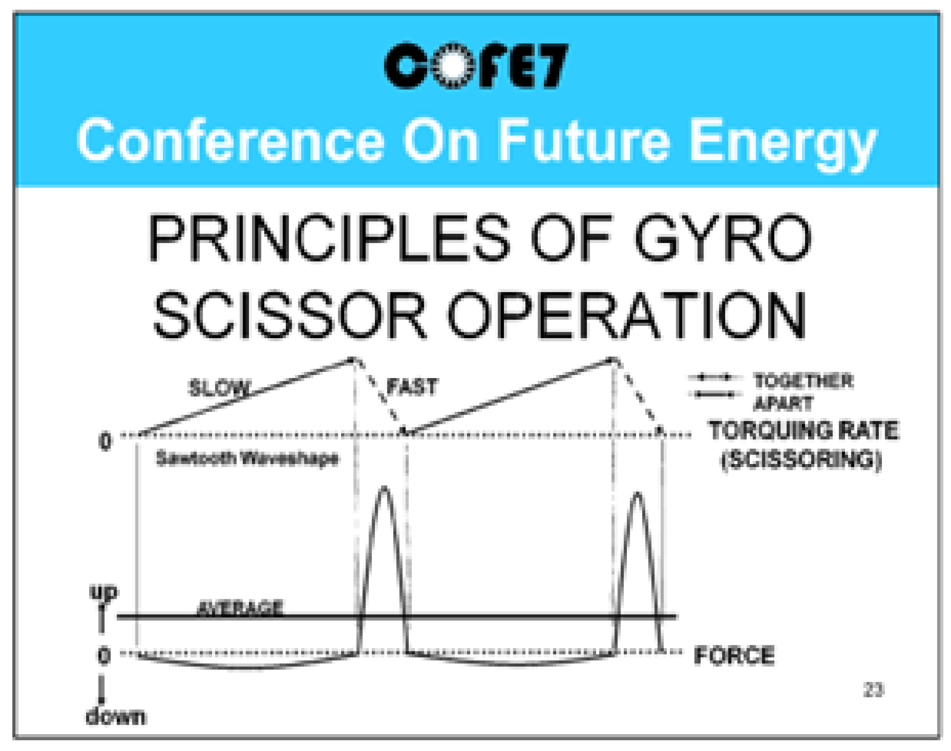
Figure 2.
Location of gyroscopes for polar angle: (a) , (b) .
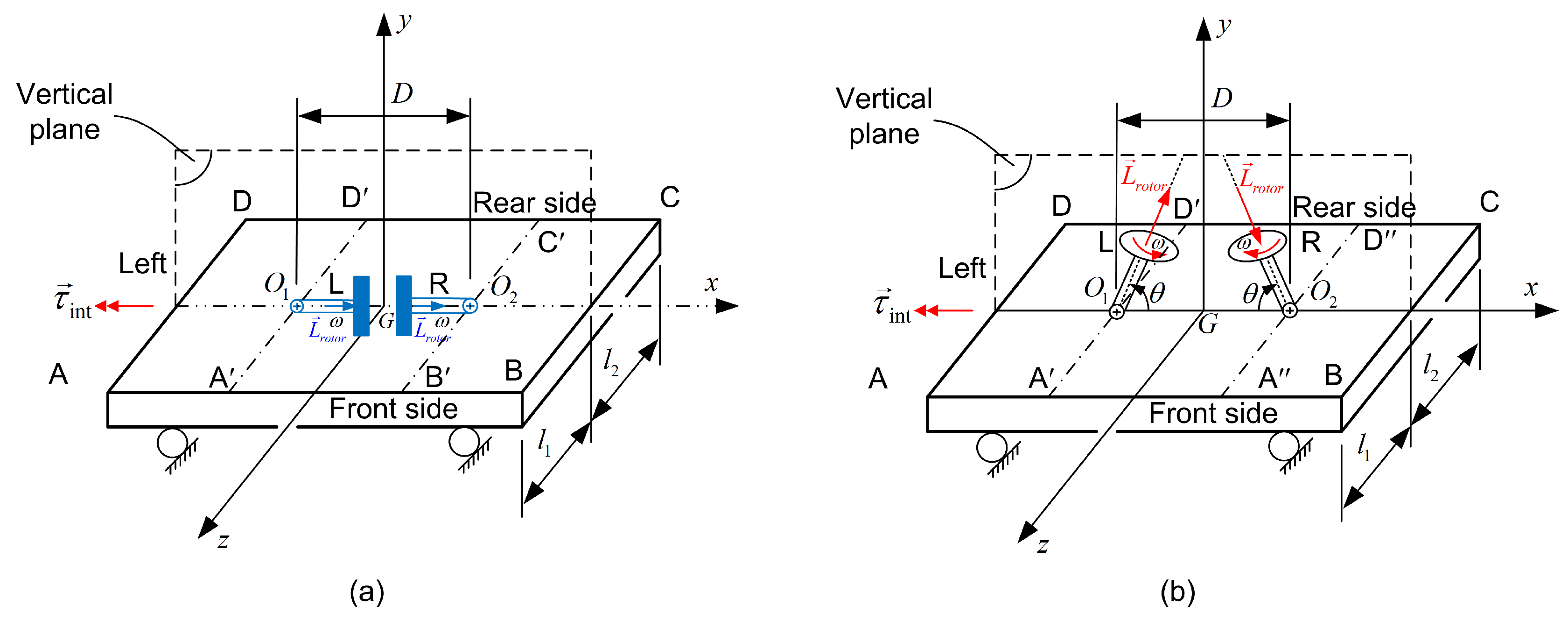
Figure 3.
Angular momenta: (a) of each contra rotating gyroscope and (b) change of the total momentum.
Figure 3.
Angular momenta: (a) of each contra rotating gyroscope and (b) change of the total momentum.
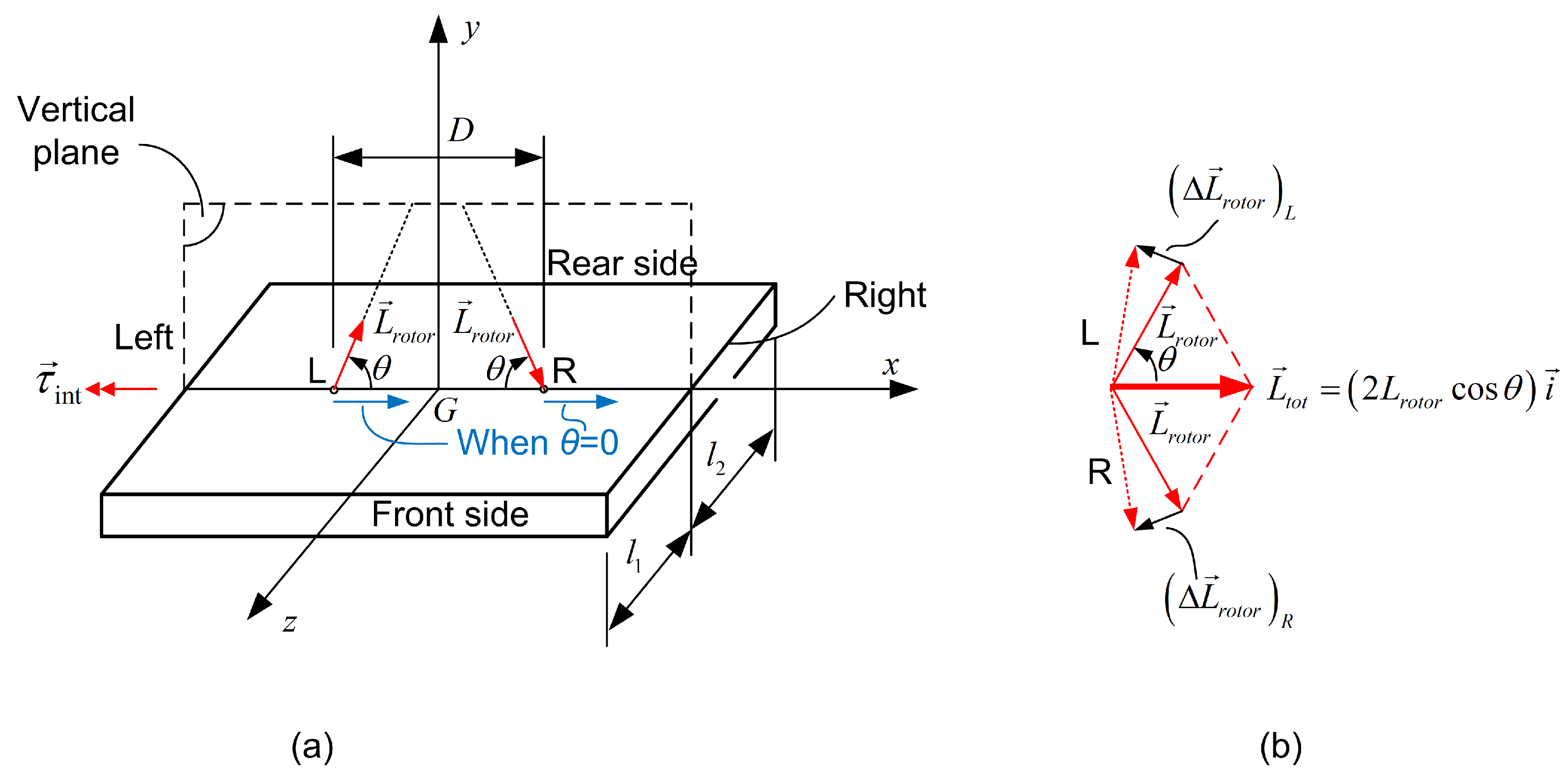
Figure 4.
Operation of gyroscopes for one period ().

Figure 5.
Sawtooth output of servo controller torquer (angle in one period: rise and reset).
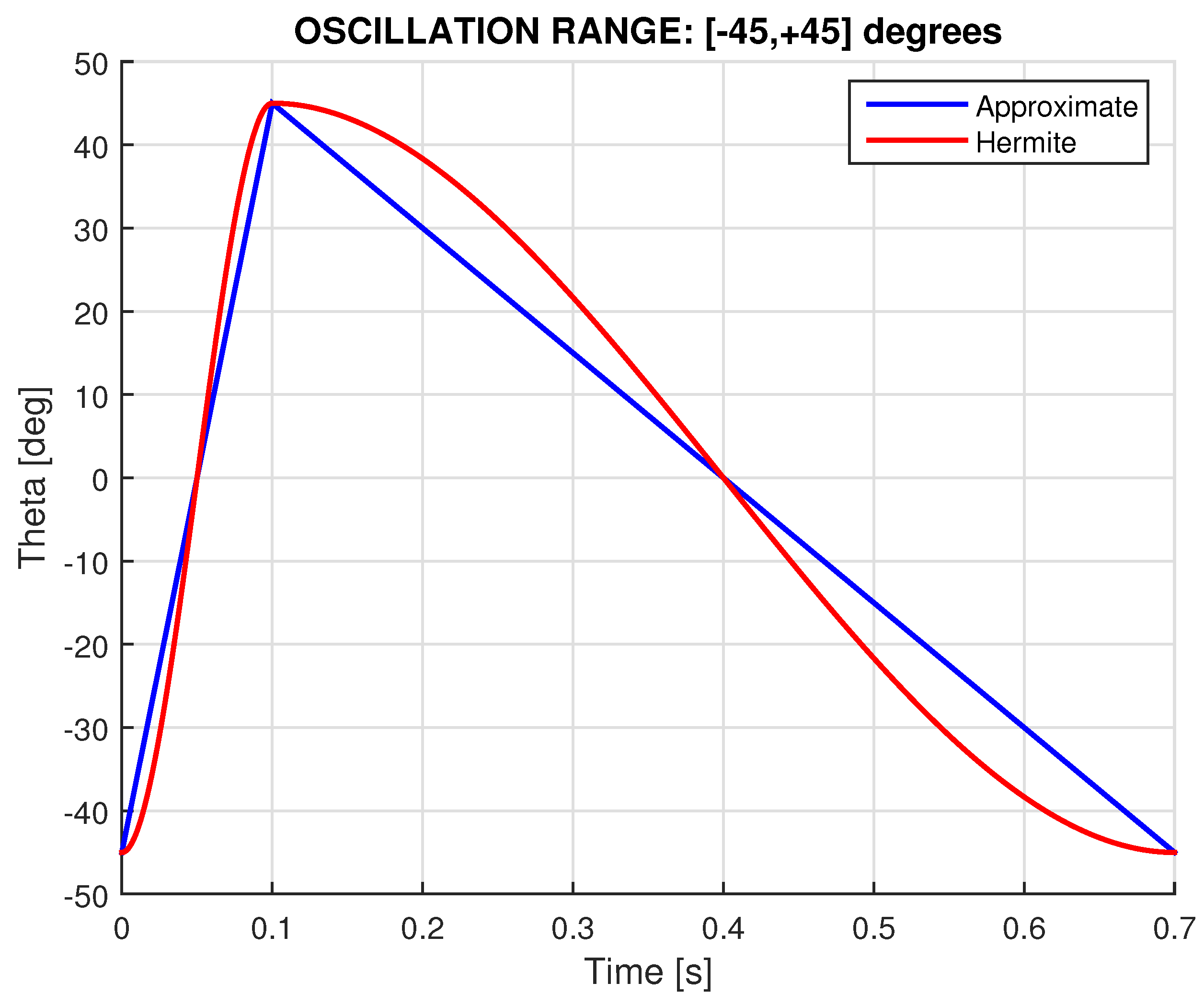
Figure 6.
Variation of the angular velocity for one period ().
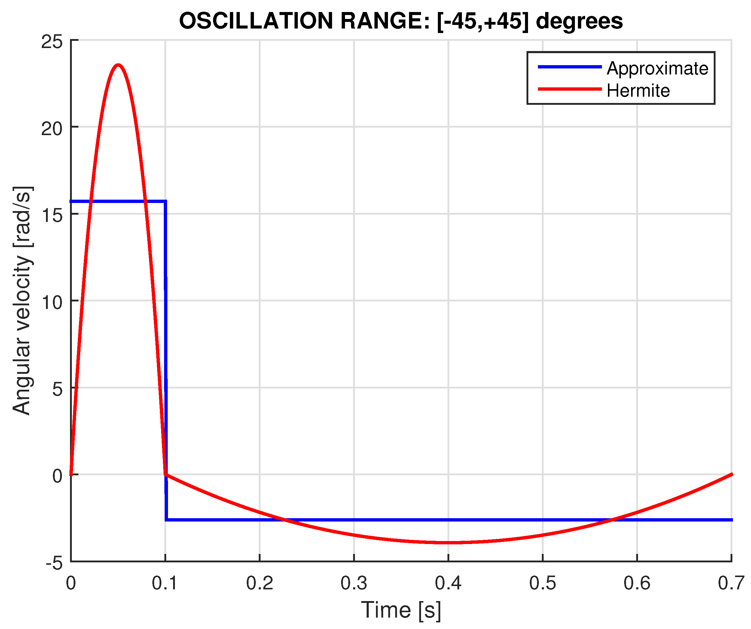
Figure 7.
Variation of the internal torque for one period, using two alternative models ().
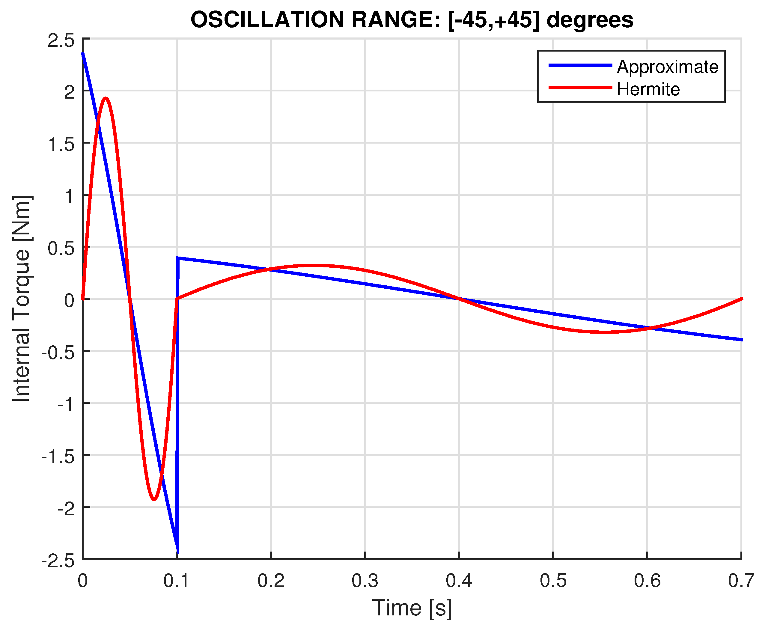
Figure 8.
Variation of the reaction forces and , due to inertial effect, for one period, using the Approximate Model ().
Figure 8.
Variation of the reaction forces and , due to inertial effect, for one period, using the Approximate Model ().
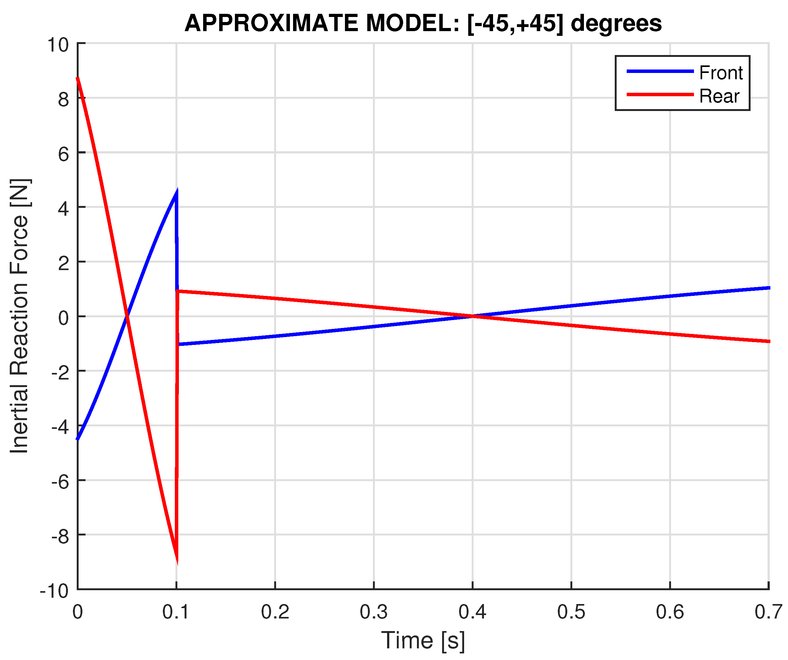
Figure 9.
Variation of the reaction forces and , due to inertial effect, for one period, using the Hermite Model ().
Figure 9.
Variation of the reaction forces and , due to inertial effect, for one period, using the Hermite Model ().
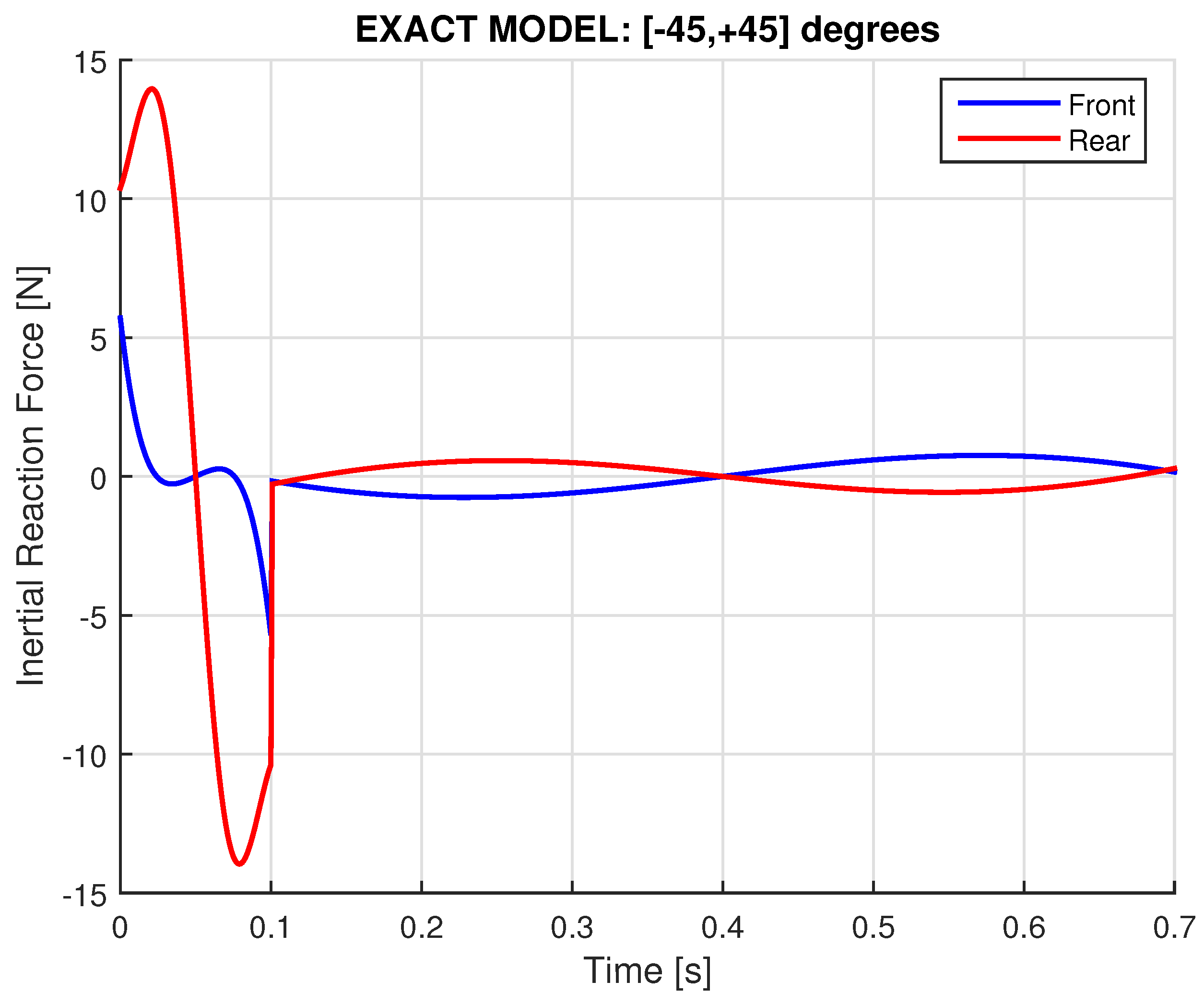
Figure 10.
Sawtooth output of servo controller torquer (angle in one period: rise and reset).
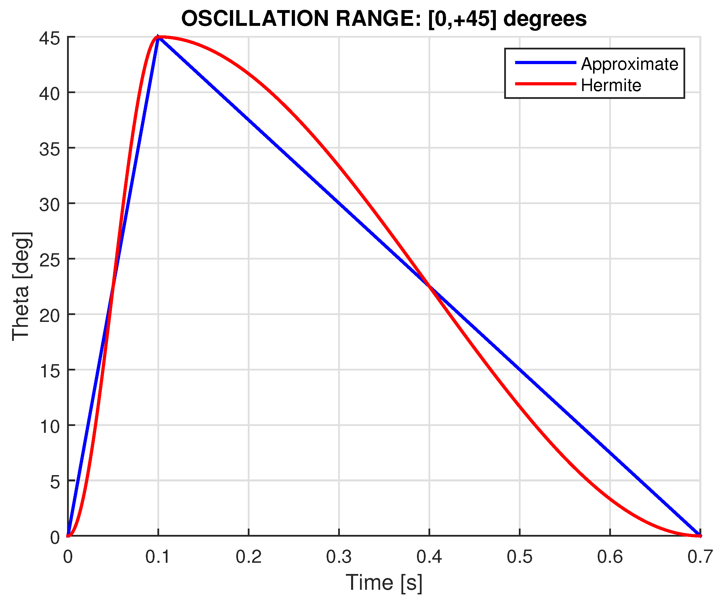
Figure 11.
Variation of the angular velocity for one period ().
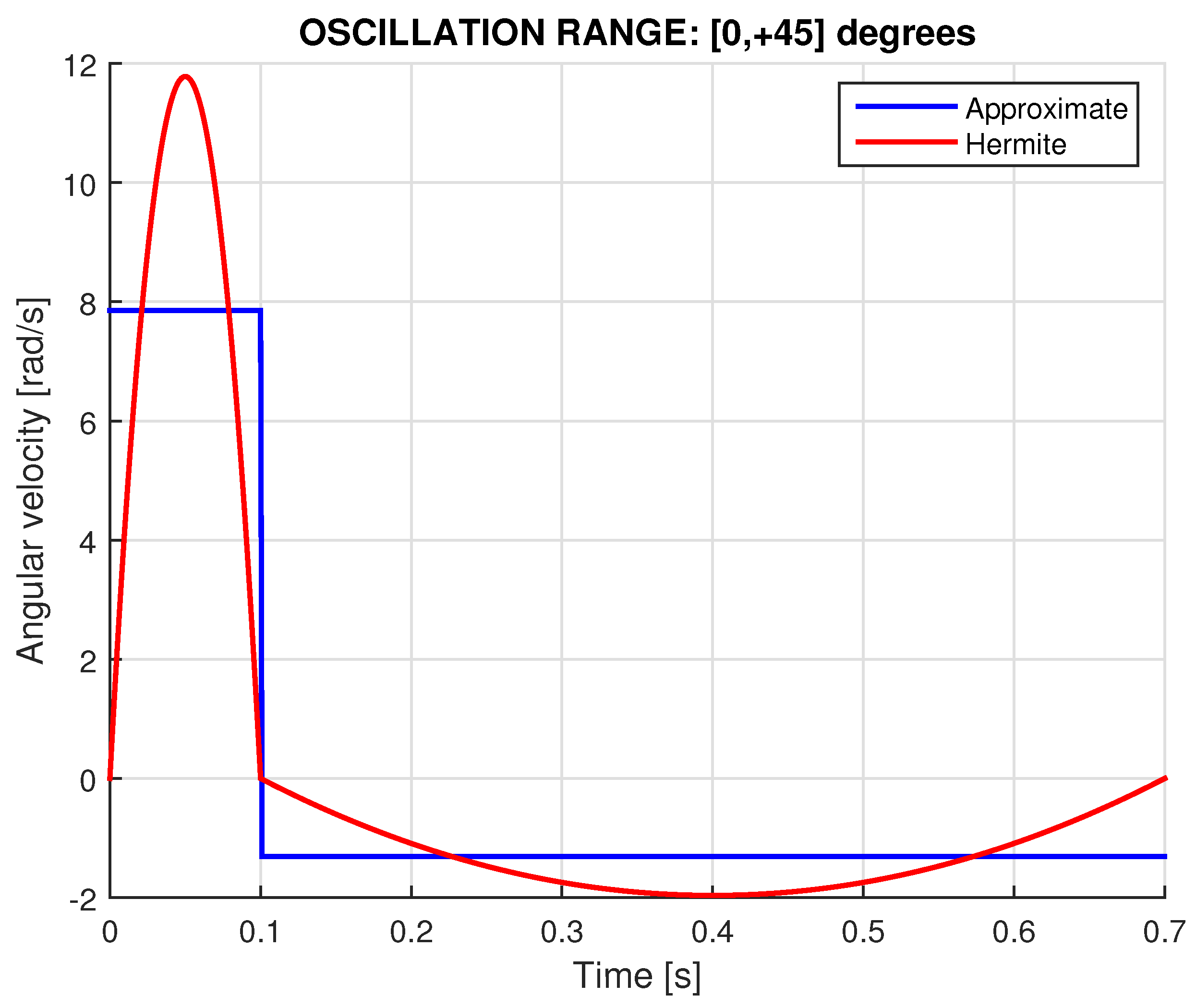
Figure 12.
Variation of the internal torque for one period, using two alternative models ().
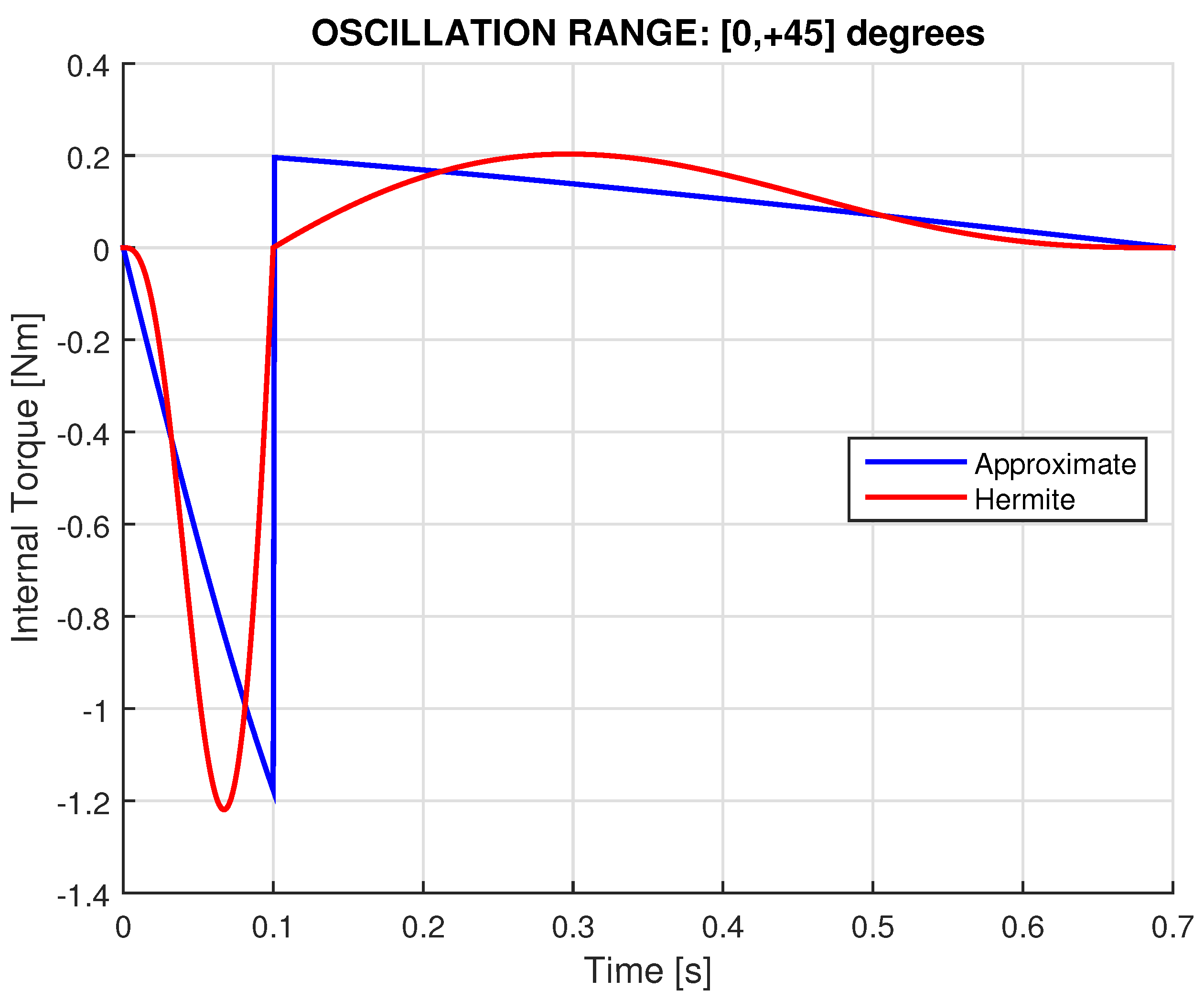
Figure 13.
Variation of the reaction forces and , due to inertial effect, for one period, using the Approximate Model ().
Figure 13.
Variation of the reaction forces and , due to inertial effect, for one period, using the Approximate Model ().
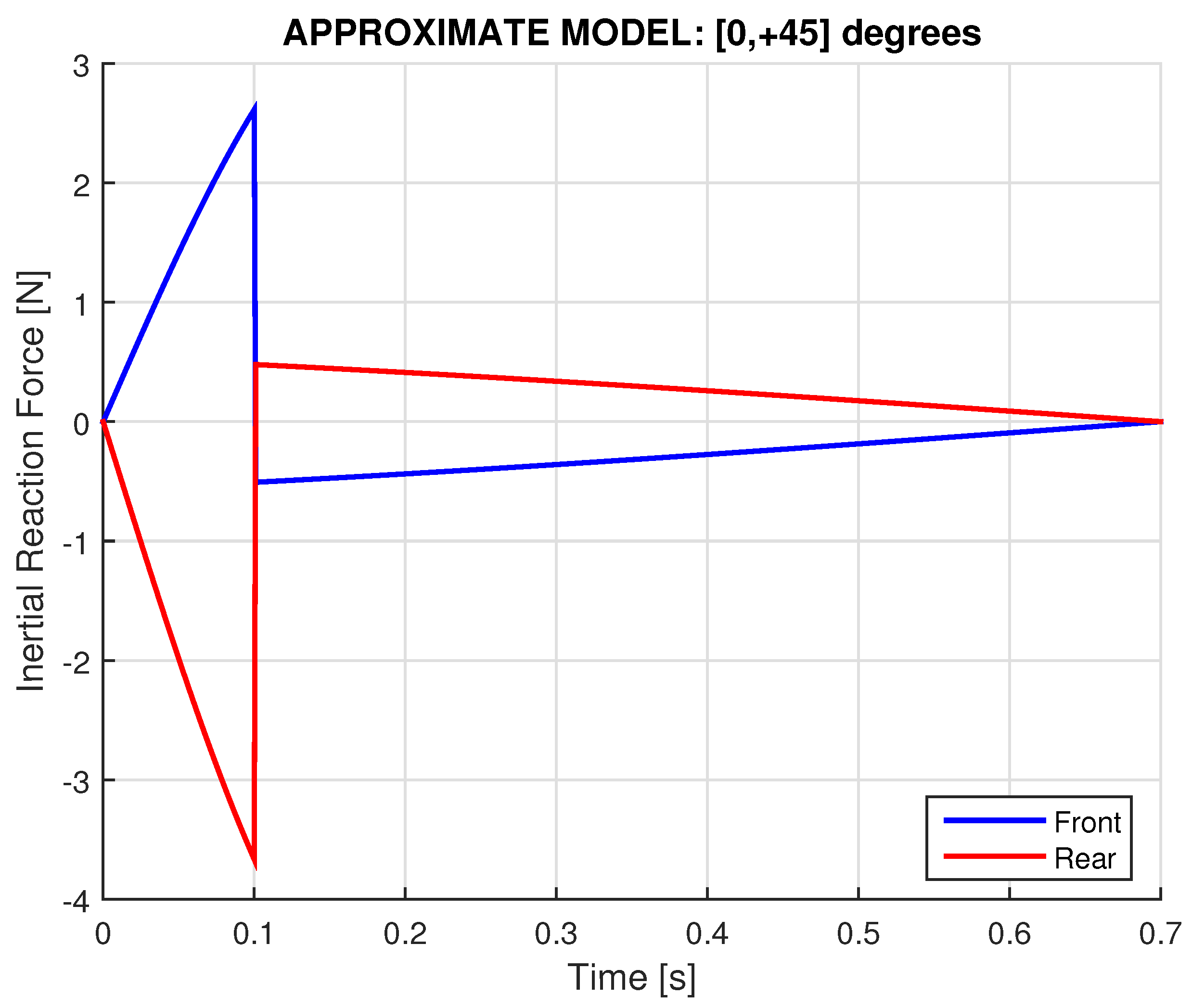
Figure 14.
Variation of the reaction forces and , due to inertial effect, for one period, using the Hermite Model ().
Figure 14.
Variation of the reaction forces and , due to inertial effect, for one period, using the Hermite Model ().
Disclaimer/Publisher’s Note: The statements, opinions and data contained in all publications are solely those of the individual author(s) and contributor(s) and not of MDPI and/or the editor(s). MDPI and/or the editor(s) disclaim responsibility for any injury to people or property resulting from any ideas, methods, instructions or products referred to in the content. |
© 2025 by the authors. Licensee MDPI, Basel, Switzerland. This article is an open access article distributed under the terms and conditions of the Creative Commons Attribution (CC BY) license (http://creativecommons.org/licenses/by/4.0/).
Copyright: This open access article is published under a Creative Commons CC BY 4.0 license, which permit the free download, distribution, and reuse, provided that the author and preprint are cited in any reuse.


