Submitted:
01 July 2025
Posted:
03 July 2025
You are already at the latest version
Abstract
A finite-horizon zero-sum linear-quadratic differential game is considered. The feature of this game is that the cost of the control of the minimizing player (the minimizer) in the game’s cost functional is much smaller than the cost of the control of the maximizing player (the maximizer) and the cost of the state variable. This smallness is due to a positive small multiplier (a small parameter) for the quadratic form of the minimizer’s control in the integrand of the cost functional. Two cases of the game's cost functional are studied: (i) the current state cost in the integrand of the cost functional is a positive definite quadratic form; (ii) the current state cost in the integrand of the cost functional is a positive semidefinite (but non-zero) quadratic form. For each of these cases, an asymptotic solution with respect to the small parameter of the considered game is formally constructed and justified. These solutions are compared with each other. Illustrative example is presented.
Keywords:
linear-quadratic differential game
; cheap control of minimizing player
; positive definite/semidefinite state cost
; singular perturbation
; asymptotic solution
1. Introduction
In this paper, a two-player finite-horizon zero-sum linear-quadratic differential game is considered. The feature of the considered game is that the control cost of the minimizer (the minimizing player) in the cost functionals is small in comparison with the cost of the state variable and with the control cost of the maximizer (the maximizing player). Such a feature means that the game under the consideration is a cheap control game. In the most general formulation, a cheap control problem is an extremal control problem in which a control cost of at least one decision maker is much smaller than a cost of the state variable in at least one cost functional of the problem.
Cheap control problems have a considerable importance in qualitative and quantitative analysis of many topics in the theory of optimal control, the theory of control and the theory of differential games. For instance, such problems are important in the following topics: (1) existence analysis and analytical/numerical computation of singular controls and arcs (see, e.g, [1,2,3,4,5,6,7,8,9,10,11,12,13,14]); (2) derivation of limiting forms and maximally achievable accuracy of optimal regulators and filters (see, e.g., [15,16,17,18,19,20,21]); (3) study of inverse optimal control problems (see e.g. [22]); (4) solution of optimal control problems with high gain control in dynamics (see, e.g., [23,24]).
The Hamilton boundary-value problem and the Hamilton–Jacobi–Bellman–Isaacs equation, associated with a cheap control problem by solvability (control optimality) conditions, are singularly perturbed because of the smallness of the control cost. This feature means that cheap control problems can be (and they really are) sources of novel classes of singularly perturbed differential equations. Thus, cheap control problems also are of considerable interest and importance in the theory of differential equations.
As it is aforementioned, in this paper we study a cheap control differential game. Cheap control differential games are extensively studied in the literature. Thus, in [12,13,14,25,26,27,28,29,30,31] various zero-sum cheap control games were analyzed. Different cheap control Nash equilibrium games were studied in [32,33,34]. A cheap control Stackelberg equilibrium differential game was studied in [35].
In most of the works, devoted to study of cheap control problems, the following two types of the quadratic cost of the "fast" state variable in the integral part of the cost functional are considered: (i) the cost is a positive definite quadratic form (see, e.g., [4,9,12,13,14,15,25,26,32,33,35] and references therein); (ii) the cost is zero (see, e.g., [27,29,31,34,36] and references therein). In the present paper, the intermediate case is studied. Namely, the case where the quadratic cost of the "fast" state variable in the integral part of the cost functional is a positive semi-definite (but non-zero) quadratic form.
More precisely, in this paper we consider the finite-horizon zero-sum linear-quadratic differential game with the cheap control of the minimizer. The dynamics of the considered game is non-homogeneous. The dimension of the minimizer’s control coincides with the dimension of the state vector and the matrix-valued coefficient of the minimizer’s control in the equation of dynamics has full rank. Hence, the entire state variable is a "fast" one. Two cases of the quadratic cost of the state variable in the integral part of the cost functional are treated, namely, (a) positive definite quadratic form and (b) positive semi-definite (but non-zero) quadratic form. Due to the solvability conditions of the game, the derivation of its state-feedback saddle-point is reduced to solution of terminal-value problems for three differential equations: matrix Riccati equation, vector linear equation and scalar trivial equation. For these differential equations with the terminal conditions, asymptotic solutions are formally constructed and justified. In the aforementioned cases (a) and (b), the algorithms of constructing the asymptotic solutions and the solutions themselves differ considerably from each other. Based on these asymptotic solutions, asymptotic approximation of the game’s value and approximate-saddle point are derived in each of the cases (a) and (b).
It should be noted the following. The cheap control differential game in the case (a) was treated in the literature (and even in more general form than in the present paper). However, to the best of our knowledge, the version of the non-homogeneous dynamics of such a game, including the derivation of an approximate-saddle point, has not yet been considered in the literature. Furthermore, to the best of our knowledge, the case (b) is completely novel. This case yields new types of singularly perturbed Riccati matrix and linear vector differential equations. For these equations, essentially novel approaches to derivation of the asymptotic solutions are proposed. Moreover, along with separate analysis of the cases (a) and (b), a comparison of the algorithms for the derivation of the aforementioned asymptotic solutions and the solutions themselves is presented. In this comparison, the case (a) serves as a reference clearly showing a considerable novelty of the case (b) and its analysis.
The paper is organized as follows. In the next section (Section 2), the cheap control differential game is rigorously formulated. Main definitions are presented. In Section 3, the non-singular (invertible) transformation of the initially formulated game is carried out. This transformation yields a new cheap control differential game which is considerably simpler than the initially formulated game. The equivalence of both games to each other is proven. It should be noted that in both games the state variable is the "fast" one. In the sequel of the paper, the new game is considered as an original cheap control differential game. In Section 4, the solvability conditions of this game are presented. These conditions contain terminal-value problems for three differential equations: matrix Riccati equation, vector linear equation and scalar trivial equation. Due to the cheap control of the minimizing player, these differential equations are perturbed by a small positive parameter . Along with the aforementioned terminal-value problems, the solvability conditions of the game contain the expressions for the components of the state-feedback saddle point and the value of the game. In Section 5, the asymptotic analysis with respect to of these solvability conditions is carried out in the case where the current state cost in the integrand of the cost functional is a positive definite quadratic form. In Section 6, such an analysis is carried out in the case where the current state cost in the integrand of the cost functional is a positive semi-definite (but non-zero) quadratic form. In both sections, the asymptotic analysis includes asymptotic solutions of the aforementioned terminal-value problems, obtaining asymptotic approximations of the game value and derivation of approximate-saddle point. In Section 7, an illustrative example is presented. Section 8 is devoted to conclusions.
The following main notations are applied in the paper.
- denotes the n-dimensional real Euclidean space;
- denotes the Euclidean norm either of a vector () or of a matrix ();
- the superscript denotes the transposition either of a vector () or of a matrix ();
- denotes the identity matrix of dimension n;
- , where , , denotes the column block-vector of the dimension with the upper block x and the lower block y;
- denotes the diagonal matrix of the dimension with the main diagonal entries ,..., ;
- denotes the space of all functions square integrable in the interval .
2. Initial Game Formulation and Main Definitions
Consider the following differential system controlled by two decision makers:
where is a state variable; and are controls of the decision makers (players); , and are given matrices of corresponding dimensions, while is a given vector of corresponding dimension; is a given constant vector; is a given time instant; the matrix-valued functions , , and the vector-valued function are continuous in the interval ; for all , .
The cost functional, to be minimized by the control w (the minimizer’s control) and maximized by the control v (the maximizer’s control ), has the form
where , and are given matrices of corresponding dimensions; for all , is symmetric and positive definite/positive semidefinite, while and are symmetric and positive definite; the matrix-valued functions , and are continuous in the interval ; is a small parameter.
We assume that both players know perfectly all the data, appearing in (1)-(2), as well as the current -position of the system (1).
Consider the set of all functions , which are measurable with respect to for any given and satisfy the local Lipschitz condition with respect to uniformly in . Similarly, let be the set of all functions , which are measurable with respect to for any given and satisfy the local Lipschitz condition with respect to uniformly in .
Based on the results of the book [14], we introduce the following definitions.
Definition 1.
By , we denote the set of all pairs , , satisfying the following conditions: (i) , ; (ii) the initial-value problem (1) for , and any has the unique absolutely continuous solution in the entire interval ; (iii) ; (iv) . We call the set of all admissible pairs of the players’ state-feedback controls in the game (1)-(2).
For a given , we consider the set
.
Let us denote
.
Similarly, for a given , we consider the set
.
Let us denote
Definition 2.
For a given , the value
is called the guaranteed result of in the game (1)-(2).
Definition 3.
For a given , the value
is called the guaranteed result of in the game (1)-(2).
Definition 4.
A pair is called a saddle-point solution of the game (1)-(2) if the guaranteed results of and in this game are equal to each other for all , i.e.,
If this equality is valid, then the value
is called a value of the game (1)-(2). The solution of the initial-value problem (1) with , is called a saddle-point trajectory of the game (1)-(2).
3. Transformation of the Differential Game (1)-(2)
In what follows, we assume that:
A1. The matrix-valued functions , , are twice continuously differentiable in the interval .
A2. The matrix-valued functions , , are three times continuously differentiable in the interval .
A3. The vector-valued function is twice continuously differentiable in the interval .
Remark 1.
By , let us denote the unique symmetric positive definite square root of the positive definite matrix , . The inverse matrix of is denoted as . It is clear that also is symmetric and positive definite. Moreover, due to the assumption A2, the matrix-valued functions and are three times continuously differentiable in the interval .
Remark 2.
Since the matrix is symmetric for all , then the matrix
also is symmetric for all . Therefore, due to the results of [38], there exists an orthogonal matrix , such that
where , are eigenvalues of the matrix . Due to the assumption A2 and the results of [39], the matrix-valued function and the functions , are three times continuously differentiable in the interval . Moreover, since the matrix is at least positive semidefinite, then , , .
Let us make the following state and control transformations in the game (1)-(2):
where is a new state variable and is a new control variable.
Since the matrices , and are invertible, then the transformations (4) and (5) are invertible.
Lemma 1.
Let the assumptions A1-A3 be valid. Then, the transformations (4) and (5) convert the system (1) and the cost functional (2) to the following system and cost functional:
where
The matrix-valued functions , and the vector-valued function are twice continuously differentiable in the interval .
Proof.
Differentiating (4) yields
Substituting this expression for , as well as (4) and (5), into the system (1), we obtain
Now, resolving the first equation in (13) with respect to , the second equation in (13) with respect to and using the orthogonality of the matrix , we directly prove the equations (6),(8)-(11).
Furthermore, substitution of (4),(5) into the cost functional (2) and use of Remark 1 and the equation (3) immediately yield the cost functional (7).
Finally, the smoothness of the matrices , , , claimed in the lemma, is a direct consequence of the equations (8)-(10) and the assumptions A1-A3. □
Remark 3.
The cost functional (7) is minimized by the control u (the minimizer’s control) and maximized by the control v (the maximizer’s control). Similarly to the game (1)-(2), we assume that in the game (6)-(7) both players know perfectly all the data, appearing in the system (6) and the cost functional (7), as well as the current -position of the system (6).
Consider the set of all functions , which are measurable with respect to for any given and satisfy the local Lipschitz condition with respect to uniformly in . Similarly, we consider the set of all functions , which are measurable with respect to for any given and satisfy the local Lipschitz condition with respect to uniformly in .
Similarly to Definitions 1-4, we introduce the following definitions.
Definition 5.
Let be the set of all pairs , , satisfying the following conditions: (i) , ; (ii) the initial-value problem (6) for , and any has the unique absolutely continuous solution in the entire interval ; (iii) ; (iv) . We call the set of all admissible pairs of the players’ state-feedback controls in the game (6)-(7).
For a given , we consider the set
.
Let us denote
.
Similarly, for a given , we consider the set
.
Let us denote
Definition 6.
For a given , the value
is called the guaranteed result of in the game (6)-(7).
Definition 7.
For a given , the value
is called the guaranteed result of in the game (6)-(7).
Definition 8.
A pair is called a saddle-point solution of the game (6)-(7) if the guaranteed results of and in this game are equal to each other for all , i.e.,
If this equality is valid, then the value
is called a value of the game (6)-(7). The solution of the initial-value problem (6) with , is called a saddle-point trajectory of the game (6)-(7).
Let and be any prechoosen vectors satisfying the equation (11).
The following assertion is a direct consequence of Definition 1, Definition 5 and Lemma 1.
Corollary 1.
Let the assumptions A1-A3 be valid. Let be an admissible pair of the players’ state-feedback controls in the game (1)-(2), i.e., . Let , be the solution of the initial-value problem (1) generated by this pair of the players’ controls. Then the pair is an admissible pair of the players’ state-feedback controls in the game (6)-(7), meaning that
. Furthermore, , , where , is the unique solution of the initial-value problem (6) generated by the players’ controls , . Moreover, . Vice versa: let and , be the solution of the initial-value problem (6) generated by this pair of the players’ controls. Then and , , where , is the unique solution of the initial-value problem (1) generated by the players’ controls , . Moreover, .
Lemma 2.
Let the assumptions A1-A3 be valid. Let the pair be a saddle-point of the game (1)-(2). Then the pairs is a saddle-point of the game (6)-(7). Vice versa: let the pair be a saddle-point of the game (6)-(7). Then the pair is a saddle-point of the game (1)-(2).
Proof.
We start with the first lemma’s statement. Since the pair is a saddle-point of the game (1)-(2), then the pair of the players’ controls is admissible in this game. Hence, due to Corollary 1, the pair of the players’ controls is admissible in the game (6)-(7) and the following equality is valid: . Moreover, by Definitions 2-3, Definitions 6-7 and Corollary 1, we obtain
The equalities in (15), along with Definitions 4 and 8, directly yield the first statement of the lemma. The second statement is proven quite similarly. □
Remark 4.
Due to Lemma 2, the initially formulated game (1)-(2) is equivalent to the new game (6)-(7). Along with this equivalence, due to Lemma 1, the latter game is simpler than the former one. Therefore, in what follows, we deal with the game (6)-(7), which we consider as an original one and call it the Cheap Control Differential Game (CCDG). In the next section, ε-dependent solvability conditions of the CCDG are presented.
Remark 5.
By the nonsingular control transformation , ( is a new control of the minimizer), the CCDG can be converted to the equivalent zero-sum differential game consisting of the dynamic system
and the cost functional
In this game, the dynamic equation is singularly perturbed and the state variable is a fast state variable (see, e.g., [37]). Therefore, we call the state variable of the CCDG a fast state variable. Thus, the cost functional contains the cost of the fast state variable , the cost of the maximizer’s control and the non small cost of the minimizer’s control , while the cost functional of the CCDG contains the cost of the fast state variable , the cost of the maximizer’s control and the small cost of the minimizer’s control .
4. Solvability Conditions of the CCDG
Consider the following matrices:
where , .
Using the data of the CCDG (see the equations (6)-(7)) and the matrices in (16), we construct the terminal-value problem for the Riccati matrix differential equation
In what follows, we assume
A4. For a given , the terminal-value problem (17) has the symmetric solution in the entire interval .
Remark 6.
Since the right-hand side of the differential equation in (17) is a smooth function with respect to the unknown matrix K, then the aforementioned solution is unique.
Using the assumption A4, as well as the data of the CCDG and the equation (16), we construct the terminal-value problem for the linear vector-valued differential equation
The problem (18) has the unique solution in the entire interval . Using this solution, we construct the terminal-value problem for the scalar differential equation
This problem has the unique solution in the entire interval .
Consider the functions
and
Proposition 1.
Let the assumptions A1-A4 be valid. Then the pair is the saddle point of the CCDG. The value of this game has the form
In the forthcoming sections, we derive an asymptotic solution of the CCDG with respect to the small parameter in the following two cases:
where , are the entries of the diagonal matrix (see the equations (3) and (7)).
We start the asymptotic solution of the CCDG with the simpler case, namely, case I.
5. Asymptotic Solution of the CCDG in the Case I
5.1. Transformation of the Terminal-Value Problems (17)-(19)
First of all, let us note the following. Due to the equation (16), the differential equations in the problems (17)-(19) have the singularities with respect to in their right-hand sides for . To remove these singularities, we look for the solutions of the problems (17) and (18) in the form
where and are new unknown matrix-valued function and vector-valued function.
Substitution of (25)-(26) into the problems (17)-(19) yields the following new terminal-value problems
Moreover, substitution of (25)-(26) into the expressions for the components of the CCDG saddle point and into the expression for the CCDG value (see the equations (20),(21) and (22)) yields the following new expressions for the components of the saddle point and for the game value:
5.2. Asymptotic Solution of the Terminal-Value Problem (27)
The problem (27) is a singularly perturbed terminal-value problem. Based on the Boundary Functions Method [37], we look for the first-order asymptotic solution of (27) in the form
where
Remark 7.
In (33), the terms with the superscript o constitute the so-call outer solution, the terms with the superscript b are the boundary corrections in the left-hand neighborhood of . Equations and boundary conditions for the asymptotic solution terms are obtained substituting into the problem (27) instead of and equating the coefficients for the same power of ε on both sides of the resulting equations, separately depending on t and on τ. Additionally, we note the following. For any and , . Moreover, if , then, for any , .
5.2.1. Obtaining the Outer Solution Term
Due to Remark 7, we have the following matrix Riccati algebraic equation for :
yielding
Remark 8.
Due to Remark 2 and the equation (23), the matrix is positive definite for all . Moreover, the matrix-valued function is three times continuously differentiable in the interval .
5.2.2. Obtaining the Boundary Correction
Taking into account Remark 7 and the equations (34),(36), we directly derive the following terminal-value problem for :
The differential equation in (37) is a matrix Bernulli differential equation [42]. Using this feature, we obtain the solution of the problem (37)
Due to the positive definiteness of , the matrix-valued function is exponentially decaying for , i.e.,
where is some constant;
5.2.3. Obtaining the Outer Solution Term
Using the equation (36) and Remark 8, we have (similarly to (35)) the matrix linear algebraic equation for
Using the results of [43] and taking into account the equations (23),(36), we obtain the solution of the equation (41)
5.2.4. Obtaining the Boundary Correction
Using Remark 7 and the equations (34),(36),(38),(42), we derive (similarly to the equation (37)) the following terminal-value problem for :
where
Due to the inequality (39), the matrix-valued function is estimated as:
where is some constant; the constant is given in (40).
Solving the problem (43) and using the results of [44] and the symmetry of the matrices , , we obtain
where, for any , the matrix-valued function is the unique solution of the problem
Solving this problem and taking into account the expressions for and (see the equations (36) and (38)), we have
where
The matrix-valued function satisfies the inequality
where is some constant; the constant is given in (40).
Using the equation (46) and the inequalities (45),(49) yields the following estimate for :
meaning that is an exponentially decaying function for .
5.2.5. Justification of the Asymptotic Solution to the Problem (27)
Similarly to the results of [14] (Lemma 4.2), we have the following lemma.
Lemma 3.
Let the assumptions A1-A3 and the case I (see the equation (23)) be valid. Then, there exist a positive number such that, for all , the terminal-value problem (27) has the unique solution in the entire interval . This solution satisfies the inequality
where is given by (33); is some constant independent of ε.
5.3. Asymptotic Solution of the Terminal-Value Problem (28)
Like the problem (27), the problem (28) is a singularly perturbed terminal-value problem. Based on the Boundary Functions Method [37], we look for the first-order asymptotic solution of (28) in the form
where the variable is given by (34); the terms in (51) have the same meaning as the corresponding terms in (33). These terms are obtained substituting and into the problem (28) instead of and , respectively, and equating the coefficients for the same power of on both sides of the resulting equations, separately depending on t and on .
5.3.1. Obtaining the Outer Solution Term
For this term, we have the following linear algebraic equation:
Since is an invertible matrix for all (see the equations (23) and (36)), then the equation (52) yields
5.3.2. Obtaining the Boundary Correction
Taking into account the equations (34),(53), we directly obtain the following terminal-value problem for :
yielding
5.3.3. Obtaining the Outer Solution Term
Using the equation (53), we have (similarly to (52)) the linear algebraic equation for
Since is an invertible matrix for all , then
5.3.4. Obtaining the Boundary Correction
Using the equations (34),(53),(55),(56), we derive (similarly to the equation (54)) the following terminal-value problem for :
Solving the problem (57), we have
where the matrix-valued function is given by (47).
Thus, using the equations (47),(48),(58), we obtain after a routine algebra
which yields the inequality
In this inequality, is some constant; the constant is given by (40).
Thus, is an exponentially decaying function for .
5.3.5. Justification of the Asymptotic Solution to the Problem (28)
Using the equations (51),(53),(55), we can rewrite the vector-valued function as:
Lemma 4.
Let the assumptions A1-A3 and the case I (see the equation (23)) be valid. Then, for all is introduced in Lemma 3), the terminal-value problem (28) has the unique solution in the entire interval . Moreover, there exists a positive number such that, for all , this solution satisfies the inequality
where is given by (61); is some constant independent of ε.
Proof.
First of all, let us note that the existence and the uniqueness of the solution to the problem (28) for all directly follow from its linearity and from the existence and the uniqueness of the solution to the problem (27) (see Lemma 3).
Proceed to the proof of the inequality (62). Let us make the transformation of the state variable in the problem (28)
where is a new state variable.
The transformation (63) converts the problem (28) to the equivalent terminal-value problem with respect to
where is given by (33), is given by (34),
Using Lemma 3, as well as the equations (56),(59),(61), we directly obtain the following estimates of and for all :
where and are some constants independent of .
Now, let us estimate . Using Lemma 3, as well as the equations (56),(57),(59),(61) and the inequalities (39),(60), we have for all
To complete the estimate of , one has to estimate the expression . Using the smoothness of (see Remark 8) and the equation (34), we obtain for any
The latter, along with the boundedness of in the interval and the inequality (60), yields
where is some constant independent of .
Thus, the inequalities (66),(67) and Lemma 3 imply immediately
where is some constant independent of .
The problem (64) can be rewritten in the equivalent integral form as:
where for any given and , the -matrix-valued function is the unique solution of the terminal-value problem
Based on the results of [45] and using the inequalities in (23) and the equation (36), we obtain the following estimate of for all :
where is some sufficiently small number; and are some constants independent of .
Applying the method of successive approximations to the equation (69), we construct the following sequence of the matrix-valued functions :
Using the inequalities (65),(68),(70), we obtain the existence of a positive number such that, for any , the sequence converges in the linear space of all -matrix-valued functions continuous in the interval . Furthermore, the following inequalities are fulfilled:
where is some constant independent of .
Due to the aforementioned convergence of the sequence , its limit is, for all , the solution of the integral equation (69) and, therefore, of the terminal-value problem (64) in the entire interval . Since the problem (64) is linear, its solution is unique. Moreover, by virtue of the inequalities in (71), we directly have
Finally, this inequality, along with the equation (63), yields the inequality (62), which completes the proof of the lemma. □
5.4. Asymptotic Solution of the Terminal-Value Problem (29)
Solving the problem (29) and taking into account Lemma 4, we obtain
Let us consider the function
Using (56), this function can be represented as:
Lemma 5.
Let the assumptions A1-A3 and the case I (see the equation (23)) be valid. Then, for all ( is introduced in Lemma 4), the following inequality is satisfied:
where is some constant independent of ε.
Proof.
Using the equations (72),(73) and taking into account the equation (61), we obtain
The latter, along with the equation (61) and the inequality (60), yields the statement of the lemma. □
5.5. Asymptotic Approximation of the CCDG value
Consider the following value, depending on :
where , and are given by (33), (51) and (73), respectively.
Using the equations (32) and (75), as well as Lemmas 3, 4, 5, we directly have the assertion.
Theorem 1.
Let the assumptions A1-A3 and the case I (see the equation (23)) be valid. Then, for all is introduced in Lemma 4), the following inequality is satisfied:
Consider the following matrix and vector:
Based on these matrix and vector, let us construct the following value, depending on :
Corollary 2.
Let the assumptions A1-A3 and the case I (see the equation (23)) be valid. Then, there exists a positive number such that, for all , the following inequality is satisfied:
where and are some constants independent of ε.
Proof.
First of all, let us note that, for (see the equation (40)) and all sufficiently small , the following inequality is valid:
This inequality, along with the equations (33),(34),(61),(76), the inequalities (39),(50),(60) and Lemmas 3, 4, yields the fulfillment of the inequalities
where is some sufficiently small number; and are some positive numbers independent of .
These inequalities and Theorem 1 directly imply the statement of the corollary. □
5.6. Approximate-Saddle Point of the CCDG
Consider the following controls of the minimizer and the maximizer, respectively:
where and are given by (33) and (61), respectively.
Remark 9.
The controls and are obtained from the controls and (see the equations (30) and (31)) by replacing there with and with .
Due to the linearity of these controls with respect to for any , and their continuity with respect to for any , , the pair is admissible in the CCDG.
Substitution of into the system (6) and the cost functional (7), as well as using the equation (16) and taking into account the symmetry of the matrix , yield after a routine algebra the following system and cost functional:
where
Based on these functions, we construct the following terminal-value problems:
where .
Remark 10.
Due to the linearity, the problem (82) has the unique solution in the entire interval for all . Therefore, the problems (83) and (84) also have the unique solutions and , respectively, in the entire interval for all .
Lemma 6.
The value , given by the equations (79)-(80), can be represented in the form
Proof of the lemma is presented in Section 5.7
Lemma 7.
Let the assumptions A1-A3 and the case I (see the equation (23)) be valid. Then, there exists a positive number ( is introduced in Lemma 4) such that, for all , the following inequality is satisfied:
where is the solution of the terminal-value problem (27) mentioned in Lemma 3; is some constant independent of ε.
Proof.
For any , let us consider the matrix-valued function
Using the problems (27) and (82), we obtain after a routine rearrangement the terminal-value problem for
where is given by (33).
Solving the problem (87) and using the results of [44], we have
where for any given and , the matrix-valued function is the unique solution of the terminal-value problem
Based on the results of [45] and using the inequalities in (23) and the equations (33),(36),(81), we obtain the following estimate of for all :
where is some sufficiently small number; and are some constants independent of .
Using the equations (16),(88), as well as Lemma 3 and the inequality (90), we directly obtain the inequality
where is some constant independent of .
Thus, the equation (86) and the inequality (91) immediately yield the statement of the lemma, which completes its proof. □
Lemma 8.
Let the assumptions A1-A3 and the case I (see the equation (23)) be valid. Then, for all ( is introduced in Lemma 7), the following inequalities are satisfied:
where and are the solutions of the terminal-value problems (28) and (29) mentioned in Lemma 4 and Lemma 5, respectively; is some constant independent of ε; the constant is introduced in Lemma 4.
Proof.
We start the proof with the inequality (92).
For any , let us consider the vector-valued function
Using the problems (28) and (83), we obtain after a routine rearrangement the terminal-value problem for
where and are given by (33) and (61), respectively.
Solving the problem (95), we have
where for any given and , the matrix-valued function is the unique solution of the terminal-value problem (89).
Using Lemmas 3, 4, 7 and the inequality (90), we obtain the inequality
where is some constant independent of .
The equation (94) and the inequality (96) directly imply the inequality (92).
Proceed to the proof of the inequality (93). From the equation (19), we have
Using the equations (16),(81),(84), we obtain
Using these expressions for and , as well as the inequalities (62) and (92), we obtain the following chain of the inequalities for all :
which directly yields the inequality (93).
Thus, the lemma is proven. □
Theorem 2.
Let the assumptions A1-A3 and the case I (see the equation (23)) be valid. Then, for all ( is introduced in Lemma 7), the following inequality is satisfied:
Proof.
The statement of the theorem directly follows from the equations (32),(85) and Lemmas 7, 8. □
Remark 11.
Due to Theorem 2, the outcome of the CCDG, generated by the pair of the controls , approximate the CCDG value with a high accuracy for all sufficiently small . This observation allows us to call the pair an approximate-saddle point in the CCDG.
5.7. Proof of Lemma 6
First, let us calculate the value using its definition, i.e., the equations (79)-(80).
Solving the initial-value problem (79), we obtain
where the -matrix-valued function is given by the equation (89). This function can be represented as:
where the -matrix-valued function is the unique solution of the terminal-value problem
Substituting (98) into (97), we obtain
Substitution this expression of into (80) yields after a routine rearrangement the following expression for :
Now, let us calculate the expression in the right-hand side of the equation (85). To do this, we should solve the terminal-value problems (82),(83) and (84).
Using (99), we obtain the solution of the problem (82) in the form
Substituting this expression for into (83) and solving the resulting problem yield after some rearrangement its solution as:
Finally, substituting the above obtained expression for into (84) and solving the resulting problem, we have its solution in the form
Let us show that can be represented as:
First, we observe that , given in (103), and the expression in the right-hand side of (104) become zero at . Differentiation of , given in (103), yields
The same expression is obtained by the differentiation of the function in the right-hand side of (104). This feature, along with the aforementioned observation, immediately yields the validity of (104).
Now, using the equation (100) and the equations (101)-(104), we obtain the following equalities:
These equalities directly yield the statement of the lemma.
6. Asymptotic Solution of the CCDG in the Case II
6.1. Transformation of the Terminal-Value Problems (17)-(19)
As it was mentioned in Section 5.1, due to the equation (16), the differential equations in the problems (17)-(19) have the singularities with respect to in their right-hand sides for . To remove these singularities, in Section 5.1 the transformations (25) and (26) of the variables in the problems (17) and (18) were proposed. These transformations are applicable in the case I of the matrix (see Remark 2 and the equation (23)). However, for the asymptotic analysis of the problems (17)-(19) in the case II (see the equation (24)), we need in another transformations allowing to remove the aforementioned singularities.
Namely, the transformation of the variable in the problem (17) is
where, for all and sufficiently small , the matrices , and are of the dimensions , and , respectively; , ; the functions , and are new unknown matrix-valued functions.
The transformation of the variable in the problem (18) is
where, for all and sufficiently small , the vectors and are of the dimensions l and , respectively; the functions and are new unknown vector-valued functions.
Let us partition the matrices , and into blocks as follows:
where the matrices , , and are of the dimensions , , and , respectively; the matrices , and are of the dimensions , and , respectively; , ; the matrix has the form
Using the equations (16),(105),(107), we can rewrite the terminal-value problem (17) in the following equivalent form:
Let us partition the vector into blocks as:
where the vectors and are of the dimensions l and , respectively.
Using the equations (16),(105),(106),(107),(111), we can rewrite the terminal-value problem (18) in the following equivalent form:
Finally, using the equations (16),(106),(107),(111), we can rewrite the terminal-value problem (19) in the following equivalent form:
6.2. Asymptotic Solution of the Terminal-Value Problem (108)-(110)
Similarly to the problem (27), the problem (108)-(110) also is singularly perturbed. However, in contrast with the former, the latter contains both, fast and slow, state variables. Namely, the state variables and , derivatives of which are multiplied by the small parameter , are fast state variables, while the state variable is a slow state variable.
Similarly to (33)-(34), we look for the first-order asymptotic solution of (108)-(110) in the form
The terms in (115) have the same meaning as the corresponding terms in (33). These terms are obtained substituting into the problem (108)-(110) instead of , and equating the coefficients for the same power of on both sides of the resulting equations, separately depending on t and on .
6.2.1. Obtaining the Boundary Correction
This boundary correction satisfies the equation
To obtain a unique solution of this equation, we need an additional condition on . By virtue of the Boundary Function Method [37], such a condition is: for . Subject to this condition, the equation (116) yields the solution
6.2.2. Obtaining the Outer Solution Terms , ,
For these terms, we have the following equations in the time-interval :
The equation (118) yields the solution
Solving the equation (119) and taking into account the invertibility of for all , we obtain
Substitution of (122) into (120) yields the following terminal-value problem with respect to :
Since is a positive definite/positive semidefinite matrix for all , then by virtue of the results of [46], the problem (123) has the unique solution in the entire interval .
6.2.3. Obtaining the Boundary Corrections and
Using the equations (121) and (122), we derive the following terminal-value problem for these corrections:
This problem consists of two subproblems, which can be solved consecutively. First, the subproblem (124) is solved. Then, using its solution , the subproblem (125) is solved. The subproblem (124) is a terminal-value problem for a Bernoulli-type matrix differential equation (see, e.g., [42]) yielding the unique solution
Substituting (126) into the subproblem of (125) and solving the obtained terminal-value problem with respect to yield
Since the matrix is positive definite, the matrix-valued functions and are exponentially decaying, i.e.,
where and are some constants;
6.2.4. Obtaining the Boundary Correction
Using the equations (117) and (122) yields after a routine algebra the equation for this boundary correction
Substituting (127) into (130) and taking into account the diagonal form of the matrix , we obtain the following differential equation for :
Solution of this equation with an unknown value is
where is the inverse matrix to the matrix .
Due to the Boundary Function Method [37], we choose the unknown matrix such that for . Thus, using (131) and taking into account the positive definiteness of the matrix , we have
implying
The latter, along with the equation (131), yields after a routine rearrangement
where .
Since is a positive definite matrix, the matrix-valued function exponentially decays for , i.e.,
where is some constant; the constant is given by (129).
6.2.5. Obtaining the Outer Solution Terms , ,
Using the equations (121), (122) and (132) we have the following equations for these terms in the time-interval :
Using the results of [43] and taking into account the equation (24), we obtain the solution of the equation (134)
Furthermore, taking into account the invertibility of the matrix for all , we obtain the solution of the equation (135)
Finally, solving the problem (136), we obtain
where the matrix-valued function satisfies the terminal-value problem
6.2.6. Obtaining the Boundary Corrections and
The correction satisfies the following terminal-value problem:
where
Due to the first inequality in (128), we can estimate the matrix-valued function as:
where is some constant; the constant is given by (129).
Solving the problem (141) and using the results of [44] and the symmetry of the matrices , , we obtain similarly to (46)
where, for any , the matrix-valued function is the unique solution of the problem
Solving this problem and taking into account the expressions for and (see the equations (121) and (126)), we have
where
The matrix-valued function satisfies the inequality
where is some constant; the constant is given in (129).
Using the equation (144) and the inequalities (143),(148), we obtain the following estimate for :
meaning that is an exponentially decaying function for .
Proceed to the correction . Using the equation (122), we obtain after some rearrangement the terminal-value problem for this correction
where
The analysis and solution of the problem (150) is similar to the above presented analysis and solution of the problem (141). Namely, the matrix-valued function can be estimated as:
where is some constant; the constant is given by (129).
The solution of the problem (150) is
where the matrix-valued function is given by (145)-(147) and satisfies the inequality (148).
Using the equation (153) and the inequalities (152),(148), we obtain the following estimate of for all :
meaning that is an exponentially decaying function for .
6.2.7. Justification of the Asymptotic Solution to the Problem (108)-(110)
Lemma 9.
Let the assumptions A1-A3 and the case II (see the equation (24)) be valid. Then, there exists a positive number such that, for all , the problem (108)-(110) has the unique solution , , in the entire interval . This solution satisfies the inequalities , , where , , are given by (115); , , are some constants independent of ε.
Proof.
Let us make the transformation of variables in the problem (108)-(110)
where , are new unknown matrix-valued functions.
Consider the block-form matrix-valued function
Substituting (155) into the problem (108)-(110), using the equations for the outer solution terms and boundary corrections (see (117)-(120),(124)-(125),(130),(134)-(136),(141),(154)) and using the expressions for the matrices , , , , (see the equations (16),(105), (107)) yield after a routine algebra the terminal-value problem for
where
the matrix-valued function is expressed in a known form by the matrix-valued functions , and ; for any , is a continuous function of ; for any and , the matrix is symmetric.
Let us represent the matrix in the block form as:
where the dimensions of the blocks are the same as the dimensions of the corresponding blocks in the matrix .
Using the inequalities (128),(133),(149),(154), we obtain the following estimates for the blocks of :
where , , are some constants independent of ; the constant is given by (129); is some sufficiently small number.
Due to the results of [44], we can rewrite the terminal-value problem (157) in the equivalent integral form
where, for any given and , the -matrix-valued function is the unique solution of the problem
Let , , and be the upper left-hand, upper right-hand, lower left-hand and lower right-hand blocks of the matrix of the dimensions , , and , respectively. By virtue of the results of [45], we have the following estimates of these blocks for all :
where is some constant independent of ; is some sufficiently small number.
Applying the method of successive approximations to the equation (160), let us consider the sequence of the matrix-valued functions given as:
where , ; the matrices have the block form
and the dimensions of the blocks in each of these matrices are the same as the dimensions of the corresponding blocks in (156).
Using the block representations of all the matrices appearing in the equation (163), as well as using the inequalities (159) and (162), we obtain the existence of a positive number such that for any the sequence converges in the linear space of all -matrix-valued functions continuous in the interval . Moreover, the following inequalities are fulfilled:
where , , are some constants independent of and j.
Thus, for any ,
is a solution of the equation (160) and, therefore, of the problem (157) in the entire interval . Moreover, this solution has the block form similar to (156) and satisfies the inequalities
Since the right-hand side of the differential equation in the problem (157) is smooth w.r.t. uniformly in , this problem cannot have more than one solution. Therefore, defined by (164) is the unique solution of the problem (157). This observation, along with the equation (155) and the inequalities in (165), proves the lemma. □
6.2.8. Comparison of the Asymptotic Solutions to the Terminal-Value Problem (17) in the Cases I and II
Comparing the asymptotic solutions of the problem (17) in the cases I and II, we can observe the following.
In the case I, the problem (17) is reduced to the singularly perturbed terminal-value problem with only fast state variable (see the equation (27)). This feature yields the uniform algorithm of constructing the entire matrix asymptotic solution and the similar form of all its entries. In particular, the outer solution terms are obtained from algebraic (not differential) equations. The zero-order (with respect to ) boundary corrections appear in all the entries of the asymptotic solution.
In the case II (in contrast with the case I), the problem (17) is reduced to the singularly perturbed terminal-value problem with two types of the state variables: two fast matrix state variables and one slow matrix state variable (see the equations (108)-(110)). In this case, the outer solution terms, corresponding to the slow state variable, are obtained from differential equations. The zero-order (with respect to ) boundary correction, corresponding to the slow state variable, equals zero. The outer solution terms, corresponding to the fast state variables, are obtained from algebraic equations. The zero-order boundary corrections, corresponding to these state variables, are not zero.
The aforementioned observation means a considerable difference in the derivation and the form of the asymptotic solutions to the problem (17) in the cases I and II.
Remark 12.
For the particular block form of the matrix , where , , , the second and third components of the solution to the problem (108)-(110) become identically zero, i.e., and . Hence, the problem (108)-(110) is reduced to the much simpler terminal-value problem
This problem has the same form as the terminal-value problem (27). The asymptotic solution of the latter can be obtained from the asymptotics of by replacing there with and with . However, for the sake of the better readability of the paper (including more clear explanation of the differences between the asymptotic analysis in the case I and in the case II), we present the case I as a separate case with the proper details.
6.3. Asymptotic Solution of the Terminal-Value Problem (112)-(113)
Similarly to the problem (28), the problem (112)-(113) also is singularly perturbed. However, in contrast with (28), the problem (112)-(113) contains not only a fast state variable but also a slow one. Namely, the state variable is a fast state variable, while the state variable is a slow state variable.
Similarly to (51), we look for the first-order asymptotic solution of (112)-(113) in the form
The terms in (166) have the same meaning as the corresponding terms in (51). These terms are obtained substituting and into the problem (112)-(113) instead of , , and , , and equating the coefficients for the same power of on both sides of the resulting equations, separately depending on t and on .
6.3.1. Obtaining the Boundary Correction
This boundary correction satisfies the equation
which, subject to the condition , yields the solution
6.3.2. Obtaining the Outer Solution Terms and
Taking into account the equation (122), these terms satisfy the following equations:
Solving these equations and taking into account that is an invertible matrix for all , we directly have
6.3.3. Obtaining the Boundary Correction
Using the equation (168) yields the terminal-value problem for
implying
6.3.4. Obtaining the Boundary Correction
Using the equations (167) and (169), we derive the equation for
which, subject to the condition , yields the solution
6.4. Obtaining the Outer Solution Terms and
Using the equations (122),(168) and (170), we have the equations for and
The equation (171) yields immediately
The terminal-value problem (172) has the unique solution in the entire interval
where the matrix-valued function is given by (140).
6.4.1. Obtaining the Boundary Correction
This correction satisfies the following terminal-value problem:
The solution of this problem is
where the matrix-valued function is given by (145)-(147) and satisfies the inequality (148). This inequality, along with the equation (175), yields
6.4.2. Justification of the Asymptotic Solution to the Problem (112)-(113)
Using the equations (166),(167),(168),(169),(170), we can rewrite the vector-valued functions and as:
Using this equation, as well as the equations (171),(172),(175) and the inequality (176), we obtain similarly to Lemma 9 the following assertion.
Lemma 10.
Let the assumptions A1-A3 and the case II (see the equation (24)) be valid. Then, for all ( is introduced in Lemma 9), the terminal-value problem (112)-(113) has the unique solution in the entire interval . Moreover, there exists a positive number such that, for all , this solution satisfies the inequalities , , , where , , are some constants independent of ε.
6.4.3. Comparison of the Asymptotic Solutions to the Terminal-Value Problem (18) in the Cases I and II
Comparing the asymptotic solutions of the problem (18) in the cases I and II, we can observe the following.
In the case I, the problem (18) is reduced (like the problem (17)) to the singularly perturbed terminal-value problem with only fast state variable (see the equation (28)). This feature yields the uniform algorithm of constructing the entire vector asymptotic solution and the similar form of all its entries. In particular, the outer solution terms are obtained from algebraic (not differential) equations. The first-order (with respect to ) boundary corrections appear in all the entries of the asymptotic solution.
In the case II (in contrast with the case I), the problem (18) is reduced (like the problem (17)) to the singularly perturbed terminal-value problem with two types of the state variables. The transformed problem has one fast vector state variable and one slow vector state variable (see the equations (112)-(113)). In this case, the outer solution terms, corresponding to the slow state variable, are obtained from differential equations. The first-order (with respect to ) boundary correction, corresponding to the slow state variable, equals zero. The outer solution terms, corresponding to the fast state variable, are obtained from algebraic equations. The first-order boundary correction, corresponding to this state variable, is not zero.
The aforementioned observation means a considerable difference in the derivation and the form of the asymptotic solutions to the problem (18) in the cases I and II.
Remark 13.
Similarly to Remark 12, for the particular block form of the matrix , where , , , the second component of the solution to the problem (112)-(113) becomes identically zero, i.e., . Due to this feature and that , , the problem (112)-(113) is reduced to the much simpler terminal-value problem
This problem has the same form as the terminal-value problem (28). The asymptotic solution of the latter can be obtained from the asymptotics of by replacing there with and with given in (47). However, for the sake of the better readability of the paper (including more clear explanation of the differences between the asymptotic analysis in the case I and in the case II), we present the case I as a separate case with the proper details.
6.5. Asymptotic Solution of the Terminal-Value Problem (114)
Solving the problem (114) and taking into account Lemma 10, we obtain
Let us consider the function
Using (173), this function can be represented as:
The following assertion is proven similarly to Lemma 5, using the equations (177),(178) and Lemma 10.
Lemma 11.
Let the assumptions A1-A3 and the case II (see the equation (24)) be valid. Then, for all ( is introduced in Lemma 10), the following inequality is satisfied:
where is some constant independent of ε.
Remark 14.
Comparison of the equation (73) and Lemma 5 with the equation (178) and Lemma 11, respectively, directly shows that the asymptotic solutions of the problem (19) in the cases I and II considerably differ from each other. However, due to Remarks 12 and 13, if , , , then the asymptotic solution of the problem (19) in the case I is obtained from the asymptotic solution of this problem in the case II by replacing with and with .
6.6. Asymptotic Approximation of the CCDG value
Consider the following value, depending on :
where is given in (158), is given by (178), and
Using the equations (22),(105),(106),(180), as well as Lemmas 9, 10 and 11, we directly have the assertion.
Theorem 3.
Let the assumptions A1-A3 and the case II (see the equation (24)) be valid. Then, for all ( is introduced in Lemma 10), the following inequality is satisfied:
where is the upper block of the vector , while is lower block of the vector .
Consider the following matrix and vector:
Based on these matrix and vector, let us construct the following value, depending on
Similarly to Corollary 2, we have the following assertion.
Corollary 3.
Let the assumptions A1-A3 and the case II (see the equation (24)) be valid. Then, there exists a positive number such that, for all , the following inequality is satisfied:
where , and , are some constants independent of ε.
6.7. Approximate-Saddle Point of the CCDG
Consider the following controls of the minimizer and the maximizer, respectively:
Remark 15.
The controls and are obtained from the controls and (see the equations (20) and (21)) by replacing there with and with .
Due to the linearity of these controls with respect to for any , and their continuity with respect to for any , , the pair is admissible in the CCDG.
Substituting into the system (6) and the cost functional (7), using the equation (16) and taking into account the symmetry of the matrix , we obtain (similarly to (79)-(81)) the following system and cost functional:
where is given in (158), and
Using these functions, we construct similarly to (82)-(84)) the following terminal-value problems:
where .
Remark 16.
Due to the linearity, the problem (186) has the unique solution in the entire interval for all . Therefore, the problems (187) and (188) also have the unique solutions and , respectively, in the entire interval for all .
Similarly to Lemma 6, we have the following assertion.
Lemma 12.
The value , given by the equations (184)-(185), can be represented in the form
Taking into account the symmetry of the matrix , let us represent this matrix in the block form as:
where the matrices , and are of the dimensions , and , respectively; ,
Lemma 13.
Let the assumptions A1-A3 and the case II (see the equation (24)) be valid. Then, there exists a positive number ( is introduced in Lemma 10) such that, for all , the following inequalities are satisfied:
where is the solution of the terminal-value problem (108)-(110); the matrix-valued function , given by (105), is the solution of the terminal-value problem (17); , , are some constants independent of ε.
Proof.
For any , let us consider the matrix-valued function
Similarly to (87), we obtain the terminal-value problem for
where is given in (158).
Solving this terminal-value problem and using the results of [44], we have
where for any given and , the matrix-valued function is the unique solution of the terminal-value problem (161); the blocks of the matrix-valued function satisfy the inequalities (162).
Using the equations (16),(105),(158),(190),(192),(193), as well as Lemma 9 and the inequalities (162), we obtain by a routine algebra the validity of the inequalities in (191) with . This completes the proof of the lemma. □
Let us represent the vector in the block form as:
where the vectors and are of the dimensions l and , respectively.
Lemma 14.
Let the assumptions A1-A3 and the case II (see the equation (24)) be valid. Then, for all ( is introduced in Lemma 13), the following inequalities are satisfied:
where is the solution of the terminal-value problem (112)-(113); the vector-valued function , given by (106), is the solutions of the terminal-value problems (18); the scalar function is the solutions of the terminal-value problem (19) and of the equivalent problem (114); , are some constants independent of ε; the constants and are introduced in Lemma 10.
Proof.
We start the proof with the inequalities (195).
For any , let us consider the vector-valued function
Similarly to (95), we obtain the terminal-value problem for
where and are given in (158) and (181), respectively.
Solving this terminal-value problem, we have
where for any given and , the matrix-valued function is the unique solution of the terminal-value problem (161); the blocks of the matrix-valued function satisfy the inequalities (162).
Using the equations (16),(105),(158),(181),(194),(197), as well as Lemmas 9, 10, Lemma 13 and the inequalities (162), we obtain by a routine algebra the validity of the inequalities in (195).
The inequality (196) is shown similarly to the inequality (93) (see the proof of Lemma 8).
Thus, the lemma is proven. □
Theorem 4.
Let the assumptions A1-A3 and the case II (see the equation (24)) be valid. Then, for all ( is introduced in Lemma 13), the following inequality is satisfied:
Proof.
The statement of the theorem directly follows from the equations (22),(189), as well as the equations (105),(106),(190),(194) and Lemmas 13, 14. □
Remark 17.
Due to Theorem 4, the outcome of the CCDG, generated by the pair of the controls , approximate the CCDG value with a high accuracy for all sufficiently small . This observation allows us to call the pair an approximate-saddle point in the CCDG.
7. Example
In this section, we consider a particular case of CCDG (see (6)-(7)) with the following data:
In this example, the symmetric matrix-valued functions and , given by the terminal-value problems (17) and (27), respectively, are of the dimension . The vector-valued functions and , given by the terminal-value problems (18) and (28), respectively, have the dimension 2.
7.1. Case I of the Matrix
In this subsection, we treat the differential game (6)-(7),(198) in the case I (see (23)), i.e., for and . We choose
We start the asymptotic solution of the differential game (6)-(7),(198),(199) with the asymptotic solution of the terminal-value problem for (see the equation (27)).
Using the equations (36),(38),(42) and the data of the example (198),(199), we directly have
Proceed to obtaining , which is based on the equations (44),(46),(47) and the data of the example (198),(199).
Using the equations (44) and (200), we obtain by a routine matrix calculations that . From (47) and (199), we have . Thus, due to (46),
From the above derived expressions for and , we can see that both matrix-valued functions exponentially decay for .
Based on the equations (33),(200),(201), let us construct the asymptotic solution of the problem (27) subject to the data (198),(199). For this purpose, we represent this matrix-valued function in the block form
The latter yields
where .
In Figure 1, the absolute errors
are depicted for along with their mutual estimate function . The figure illustrates Lemma 3.
Proceed to construction of the asymptotic solution to the terminal-value problem (28) subject to the data (198),(199).
Using the equations (53),(55),(56),(59) and the equation (48), we obtain
Using these results, as well as the equation (51) and the block representation of the vector-valued function
we obtain
where (like in (203)) .
In Figure 2, the absolute errors
are depicted for along with their mutual estimate function . The figure illustrates Lemma 4.
To complete the construction of the asymptotic solutions to the terminal-value problems, associated with the solvability conditions of the CCDG, we should construct the asymptotic solution to the problem (29) subject to the data (198),(199). Using the equation (74), we directly obtain
In Figure 3, the absolute error
is depicted for along with the estimate function . The figure illustrates the inequality (74) in Lemma 5 with .
Now, using the equations (75),(77), as well as the equations (202)-(203),(204)-(205),(206) and the data (198), we obtain the following two approximations of the CCDG value:
The components of the approximate-saddle point have the form (78), where is given by (202)-(203), is given by (204)-(205), , .
The game value , the values , and the outcome of the game , generated by the approximate-saddle point, are shown in Table 1 for (the initial state position is fixed by (198) yielding the simplified notation). Note that and are not distinguishable because the differences
are negligible small (, , and , respectively).
In Table 2, the absolute and the relative errors of the game value approximations in the case I
are presented. It is seen that all errors decrease with decreasing . The approximation , calculated by employing the approximate-saddle point controls, is more accurate than and (which accuracies are identical). The relative errors are not larger than for and , and not larger than for .
7.2. Case II of the Matrix
In this subsection, we treat the differential game (6)-(7),(198) in the case II (see (24)), i.e., for and . We choose
We start the asymptotic solution of the differential game (6)-(7),(198),(207) with the asymptotic solution of the terminal-value problem for (see the equations (108)-(110)).
Using the equations (117),(121),(122), we directly have
To obtain , we should solve the terminal-value problem (120) subject to the data (198),(207). This, problem has the form
yielding the unique solution
Subject to the data (198),(207), the equations (126),(127),(131) yield
Furthermore, using the equations (137)-(140) and the data (198),(207), we obtain
where is the solution of the terminal-value problem
Finally, using the equations (142),(144),(146),(147),(151),(153) and taking into account the data (198),(207) and the equations (210)-(211), we derive and
Thus, due to the equations (115),(208)-(213), we obtain the asymptotic solution of the problem (108)-(110) subject to the data (198),(207)
where .
In Figure 4, the absolute errors
are depicted for along with their mutual estimate function . The figure illustrates Lemma 9.
Proceed to construction of the asymptotic solution to the terminal-value problem (112)-(113) subject to the data (198),(207).
Using the equations (167),(168),(169),(170),(173),(174),(175) we directly have
where is the solution of the terminal-value problem (212); is given by (209).
Thus, due to the equations (166),(215), we obtain the asymptotic solution of the problem (112)-(113) subject to the data (198),(207)
where .
In Figure 5, the absolute errors
are depicted for along with their mutual estimate function . The figure illustrates Lemma 10.
Using the equation (178) and the equation (215), we obtain the asymptotic solution of the problem (114) subject to the data (198),(207)
In Figure 6, the absolute error
is depicted for along with the estimate function . The figure illustrates the inequality (179) in Lemma 11 with .
Now, using the equations (180),(182),(214),(216),(217) and the data (198), we obtain the following two approximations of the CCDG value:
Due to the equation (183) and the data (198), the components of the approximate-saddle point have the form
where , are given in (214); , are given in (216); and are upper and lower scalar blocks, respectively, of the state vector z.
The values of , , and the outcome of the game , generated by the approximate-saddle point, are shown in Table 3 for In this case, the difference between and is also negligible.
The absolute and the relative errors of the game value approximations in the Case II
are presented in Table 4.
It is seen that all errors decrease with decreasing . The approximation , calculated by employing approximate-saddle point controls, is more accurate than and (which accuracies are identical). The relative errors are not larger than for and , and not larger than for .
8. Conclusions
In this paper, a two-player finite-horizon zero-sum linear-quadratic differential game was studied in the case where the control cost of the minimizing player (the minimizer) in the cost functional is much smaller than the state cost and the cost of the control of the maximazing player. This smallness is represented by the presence of the small multiplier in the control cost of the minimizer. Due to this feature of the minimizer’s control cost, the considered game is a cheap control game. The differential equation of the considered game is non-homogeneous. The dimension of the minimizer’s control equals to the dimension of the state vector and the matrix-valued coefficient of the minimizer’s control in the differential equation has full rank. This means that the entire state variable is a "fast" one. For this game, the state-feedback saddle point and the value were sought. By the proper changes of the state and minimizer’s control variables, the initially formulated game was transformed equivalently to the much simpler zero-sum cheap control differential game. In this new game, the matrix-valued coefficient of the minimizer’s control in the differential equation is the identity matrix. The matrix-valued coefficient for the state cost in the integral part of the game’s cost functional is a diagonal one. In the sequel of the paper, this new game was considered as an original cheap control game. The following two cases of the matrix-valued coefficient for the state cost in the integral part of the game’s cost functional were treated: (a) all the entries of the main diagonal are positive; (b) only part of the entries are positive, while the rest of the entries are zero. In each of the cases, the asymptotic analysis with respect to the small parameter of the state-feedback solution in the original cheap control game was carried out. This analysis includes: (i) the first-order asymptotic solutions of the terminal-value problems for the three differential equations, appearing in the game’s solvability conditions; (ii) obtaining asymptotic approximations of the game value; (iii) derivation of approximate-saddle point. The approaches to this analysis in the cases (a) and (b) and the results of this analysis were compared with each other. This comparison clearly shows the essential novelty of the case (b) and its analysis. The analysis of the case (b) clearly shows that the assumption on the positive definiteness of the quadratic cost of the "fast" state variable in the integral part of the cost functional is not necessary. Positive semi-definiteness of this quadratic cost is not an obstacle in the asymptotic analysis of the cheap control game. Along with this, the property of this quadratic cost (positive definiteness or positive semi-definiteness) effects considerably on the asymptotic solution of the cheap control game.
References
- O’Malley, R.E. Cheap control, singular arcs, and singular perturbations. In Optimal Control Theory and its Applications; Kirby, B.J. Ed.; Lecture Notes in Economics and Mathematical Systems, Volume 106; Springer: Berlin, Heidelberg, Germany, 1974.
- Bell, D.J.; Jacobson, D.H. Singular Optimal Control Problems; Academic Press: Cambridge, MA, USA, 1975.
- O’Malley, R.E. The singular perturbation approach to singular arcs. In International Conference on Differential Equations; Antosiewicz, H.A., Ed.; Elsevier Inc.: Amsterdam, Netherlands, 1975, pp. 595–611.
- O’Malley, R.E.; Jameson, A. Singular perturbations and singular arcs, I. IEEE Trans. Automat. Control 1975, 20, 218–-226.
- O’Malley, R.E. A more direct solution of the nearly singular linear regulator problem. SIAM J. Control Optim. 1976,14, 1063–1077.
- O’Malley, R.E.; Jameson, A. Singular perturbations and singular arcs, II. IEEE Trans. Automat. Control 1977, 22, 328–-337.
- Kurina, G.A. A degenerate optimal control problem and singular perturbations. Soviet Math. Dokl. 1977, 18, 1452–-1456.
- Sannuti, P.; Wason, H.S. Multiple time-scale decomposition in cheap control problems – singular control. IEEE Trans. Automat. Control 1985, 30, 633–-644. [CrossRef]
- Saberi, A.; Sannuti, P. Cheap and singular controls for linear quadratic regulators. IEEE Trans. Automat. Control 1987, 32, 208–-219. [CrossRef]
- Smetannikova, E.N.; Sobolev, V.A. Regularization of cheap periodic control problems. Automat. Remote Control 2005, 66, 903–-916. [CrossRef]
- Glizer, V.Y. Stochastic singular optimal control problem with state delays: Regularization, singular perturbation, and minimizing sequence. SIAM J. Control Optim. 2012, 50, 2862–-2888. [CrossRef]
- Glizer, V.Y. Saddle-point equilibrium sequence in one class of singular infinite horizon zero-sum linear-quadratic differential games with state delays. Optimization 2019, 68, 349–384. [CrossRef]
- Shinar, J.; Glizer, V.Y.; Turetsky, V. Solution of a singular zero-sum linear-quadratic differential game by regularization. Int. Game Theory Rev. 2014, 16, 1–-32. [CrossRef]
- Glizer, V.Y.; Kelis, O. Singular Linear-Quadratic Zero-Sum Differential Games and H∞ Control Problems: Regularization Approach; Birkhauser: Basel, Switzerland, 2022.
- Kwakernaak, H.; Sivan, R. The maximally achievable accuracy of linear optimal regulators and linear optimal filters. IEEE Trans. Autom. Control 1972, 17, 79–-86. [CrossRef]
- Francis, B. The optimal linear-quadratic time-invariant regulator with cheap control. IEEE Trans. Autom. Control 1979, 24, 616–621. [CrossRef]
- Saberi, A.; Sannuti, P. Cheap control problem of a linear uniform rank system: Design by composite control. Automatica 1986, 22, 757–759. [CrossRef]
- Lee, J.T.; Bien, Z.N. A quadratic regulator with cheap control for a class of nonlinear systems. J. Optim. Theory Appl. 1987, 55, 289-–302. [CrossRef]
- Braslavsky, J.H.; Seron, M.M.; Mayne, D.Q.; Kokotovic, P.V. Limiting performance of optimal linear filters. Automatica 1999, 35, 189–-199. [CrossRef]
- Seron, M.M.; Braslavsky, J.H.; Kokotovic, P.V.; Mayne, D.Q. Feedback limitations in nonlinear systems: From Bode integrals to cheap control. IEEE Trans. Autom. Control 1999, 44, 829–-833. [CrossRef]
- Glizer, V.Y.; Kelis, O. Asymptotic properties of an infinite horizon partial cheap control problem for linear systems with known disturbances. Numer. Algebra Control Optim. 2018, 8, 211–-235. [CrossRef]
- Moylan, P.J.; Anderson, B.D.O. Nonlinear regulator theory and an inverse optimal control problem. IEEE Trans. Autom. Control 1973, 18, 460–-465. [CrossRef]
- Young, K.D.; Kokotovic, P.V.; Utkin, V.I. A singular perturbation analysis of high-gain feedback systems. IEEE Trans. Autom. Control 1977, 22, 931–-938. [CrossRef]
- Kokotovic, P.V.; Khalil, H.K.; O’Reilly, J. Singular Perturbation Methods in Control: Analysis and Design; Academic Press: London, UK, 1986.
- Petersen, I.R. Linear-quadratic differential games with cheap control. Syst. Control Lett. 1986, 8, 181–-188. [CrossRef]
- Glizer, V.Y. Asymptotic solution of zero-sum linear-quadratic differential game with cheap control for the minimizer. NoDEA Nonlinear Diff. Equ. Appl. 2000, 7, 231–-258. [CrossRef]
- Turetsky, V.; Shinar, J. Missile guidance laws based on pursuit—evasion game formulations. Automatica 2003, 39, 607–-618. [CrossRef]
- Turetsky, V. Upper bounds of the pursuer control based on a linear-quadratic differential game. J. Optim. Theory Appl. 2004, 121, 163–-191. [CrossRef]
- Turetsky, V.; Glizer, V.Y. Robust solution of a time-variable interception problem: A cheap control approach. Int. Game Theory Rev. 2007, 9, 637–-655. [CrossRef]
- Turetsky, V.; Glizer, V.Y.; Shinar, J. Robust trajectory tracking: Differential game/cheap control approach. Int. J. Systems Sci. 2014, 45, 2260–-2274. [CrossRef]
- Turetsky, V.; Glizer, V.Y. Cheap control in a non-scalarizable linear-quadratic pursuit-evasion game: Asymptotic analysis. Axioms 2022, 11, 214. [CrossRef]
- Glizer, V.Y. Nash equilibrium sequence in a singular two-person linear-quadratic differential game. Axioms 2021, 10, 132. [CrossRef]
- Glizer, V.Y. Nash equilibrium in a singular infinite horizon two-person linear-quadratic differential game. Pure Appl. Funct. Anal. 2022, 7, 1657–1698.
- Glizer, V.Y. Solution of one class of singular two-person Nash equilibrium games with state and control delays: regularization approach. Appl. Set-Valued Anal. Optim. 2023, 5, 401–438.
- Glizer, V.Y.; Turetsky, V. One class of Stackelberg linear-quadratic differential games with cheap control of a leader: asymptotic analysis of open-loop solution. Axioms 2024, 13, 801. [CrossRef]
- Glizer, V.Y. Solution of a singular minimum energy control problem for time delay system: regularization approach. Pure Appl. Funct. Anal. 2023, 8, 1413-1435.
- Vasil’eva, A.B.; Butuzov, V.F.; Kalachev, L.V. The Boundary Function Method for Singular Perturbation Problems; SIAM Books: Philadelphia, PA, USA, 1995.
- Bellman, R. Introduction to Matrix Analysis; SIAM Books: Philadelphia, PA, USA, 1997.
- Sibuya, Y. Some global properties of matrices of functions of one variable. Math. Annalen 1965, 161, 67–-77. [CrossRef]
- Basar, T.; Olsder, G.J. Dynamic Noncooperative Game Theory; Academic Press: London, UK, 1992.
- Zhukovskii, V.I. Analytic design of optimum strategies in certain differential games. I. Autom. Remote Control 1970, 4, 533-–536.
- Derevenskii, V.P. Matrix Bernoulli equations, I. Russiam Math. 2008, 52, 12–-21. [CrossRef]
- Gajic, Z.; Qureshi, M.T.J. Lyapunov Matrix Equation in System Stability and Control; Dover Publications: Mineola, NY, USA, 2008.
- Abou-Kandil, H.; Freiling, G.; Ionescu, V.; Jank, G. Matrix Riccati Equations in Control and Systems Theory; Birkhauser: Basel, Switzerland, 2003.
- Glizer, V.Y. Asymptotic solution of a cheap control problem with state delay. Dynam. Control 1999, 9, 339–-357. [CrossRef]
- Kwakernaak, H.; Sivan, R. Linear Optimal Control Systems; Wiley-Interscience: New York, NY, USA, 1972.
Figure 1.
Absolute errors of the asymptotic expansion of .
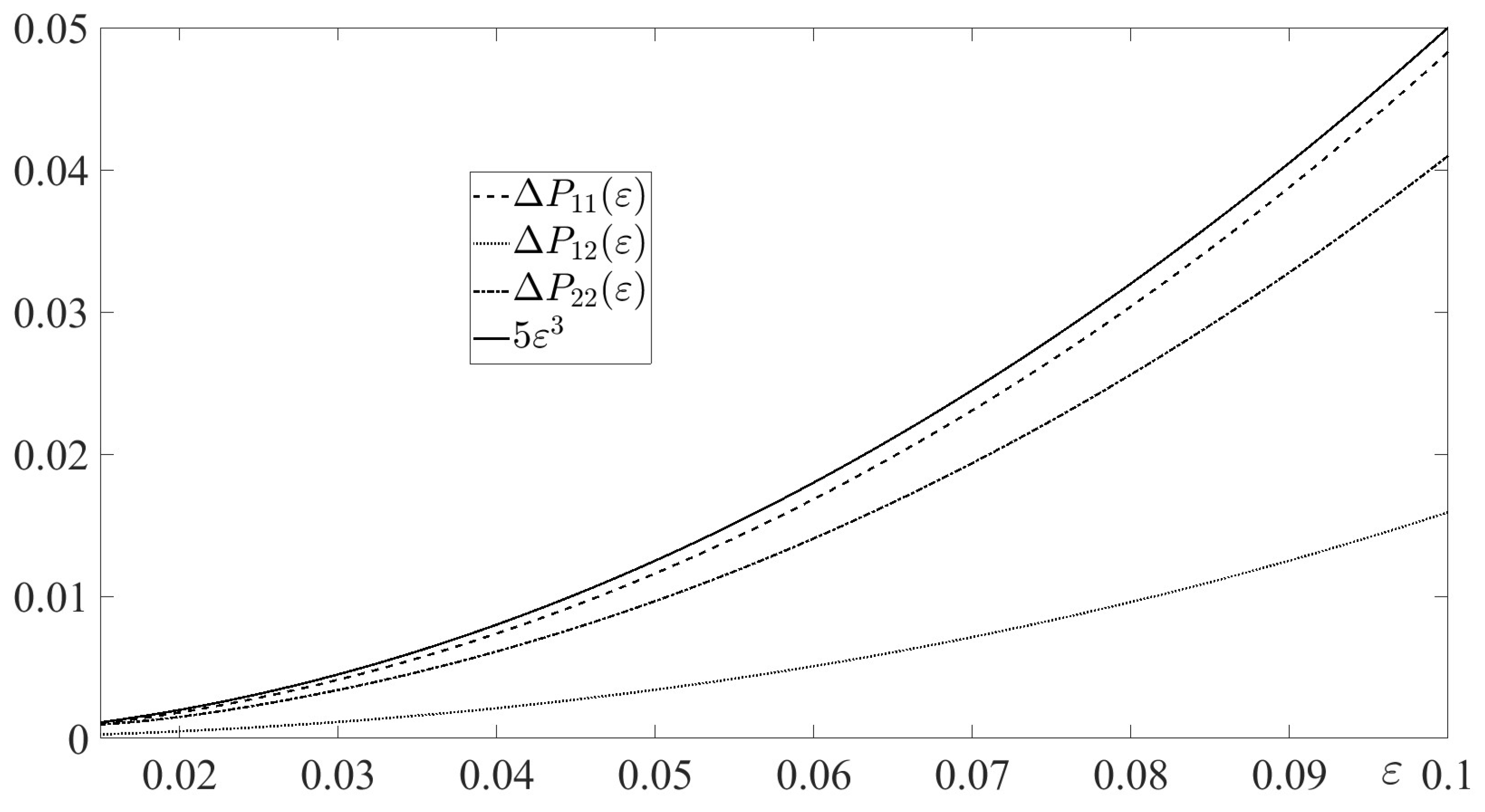
Figure 2.
Absolute errors of the asymptotic expansion of .
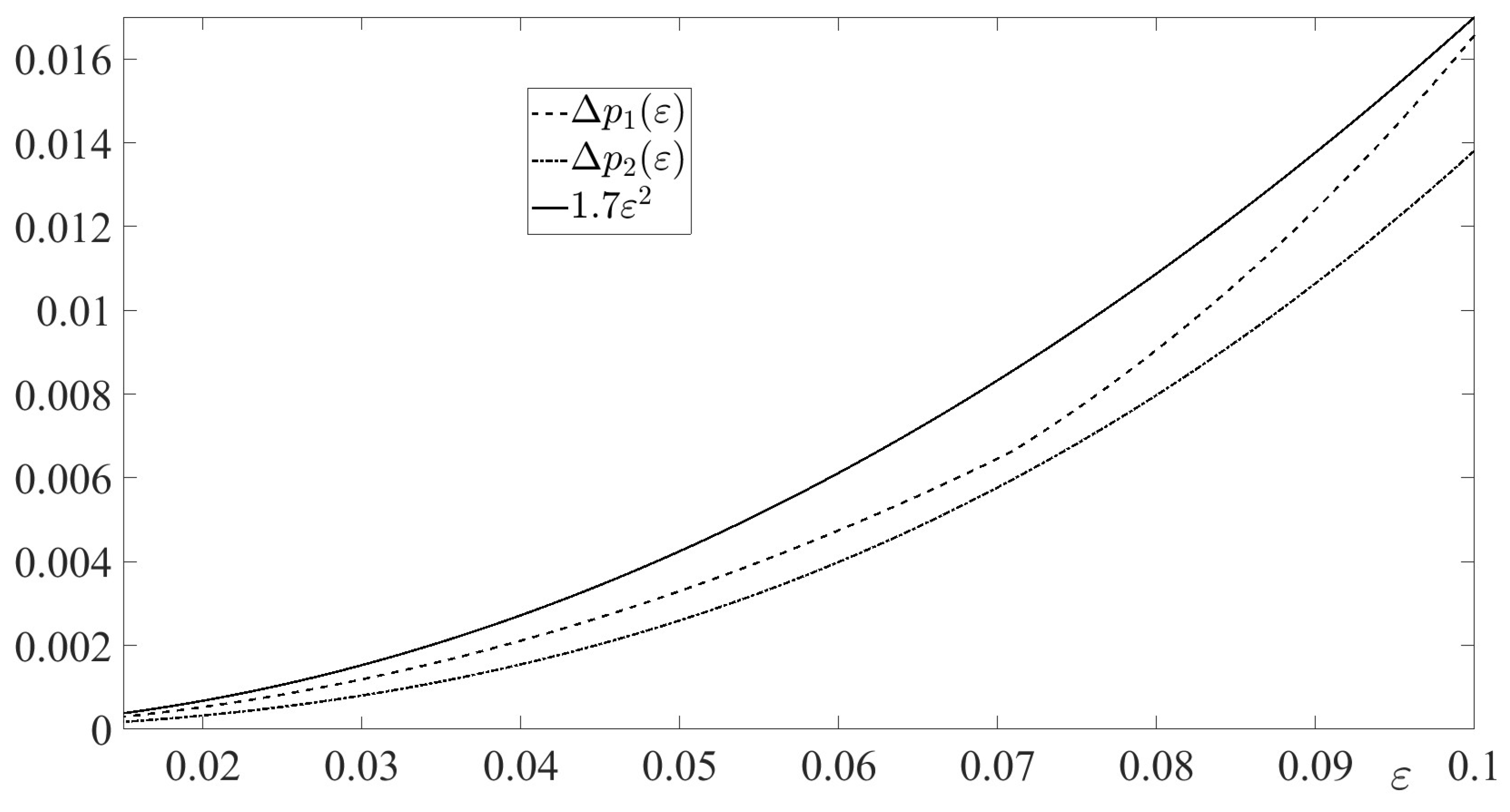
Figure 3.
Absolute errors of the asymptotic expansion of .
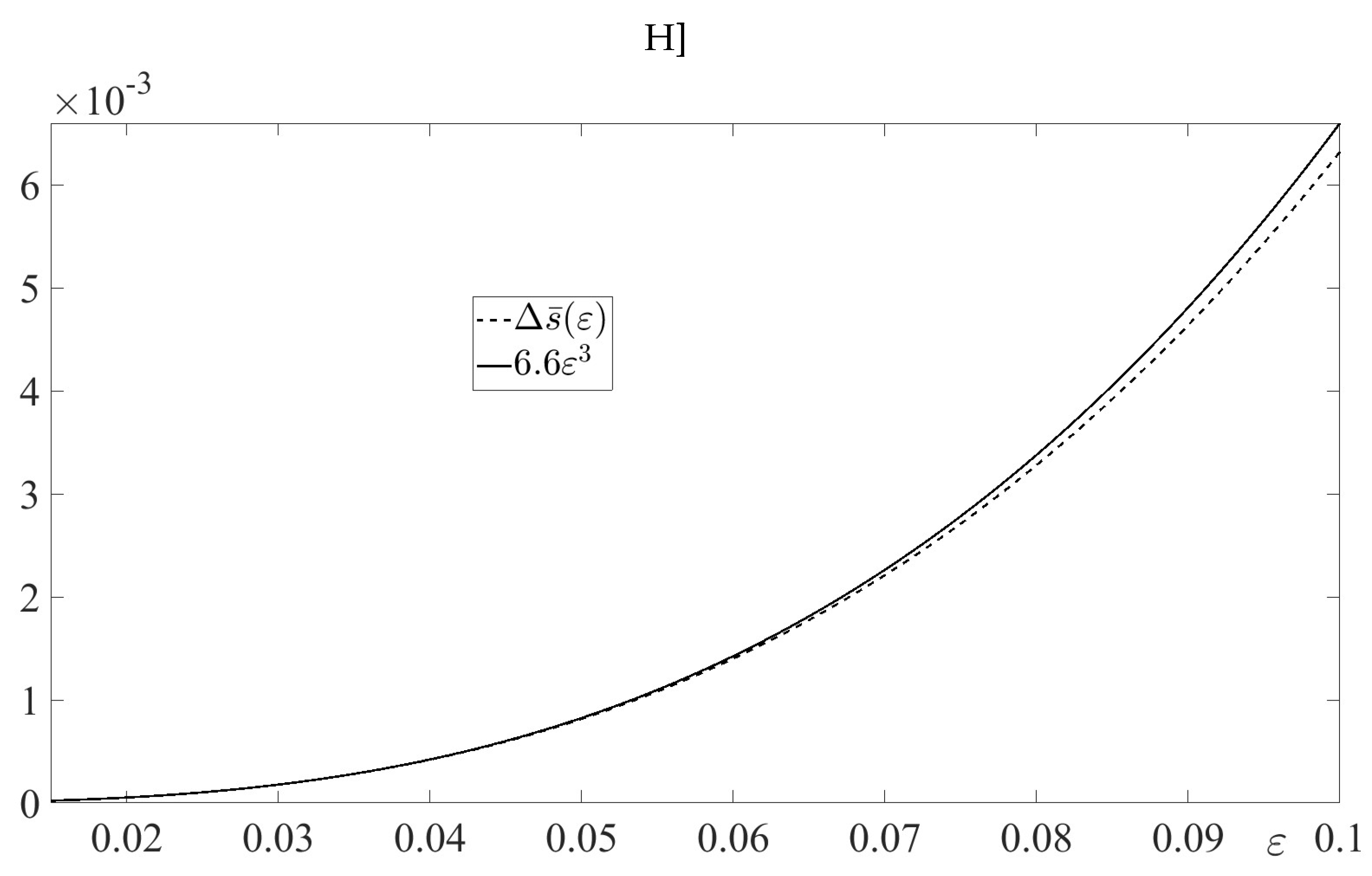
Figure 4.
Absolute errors , and .
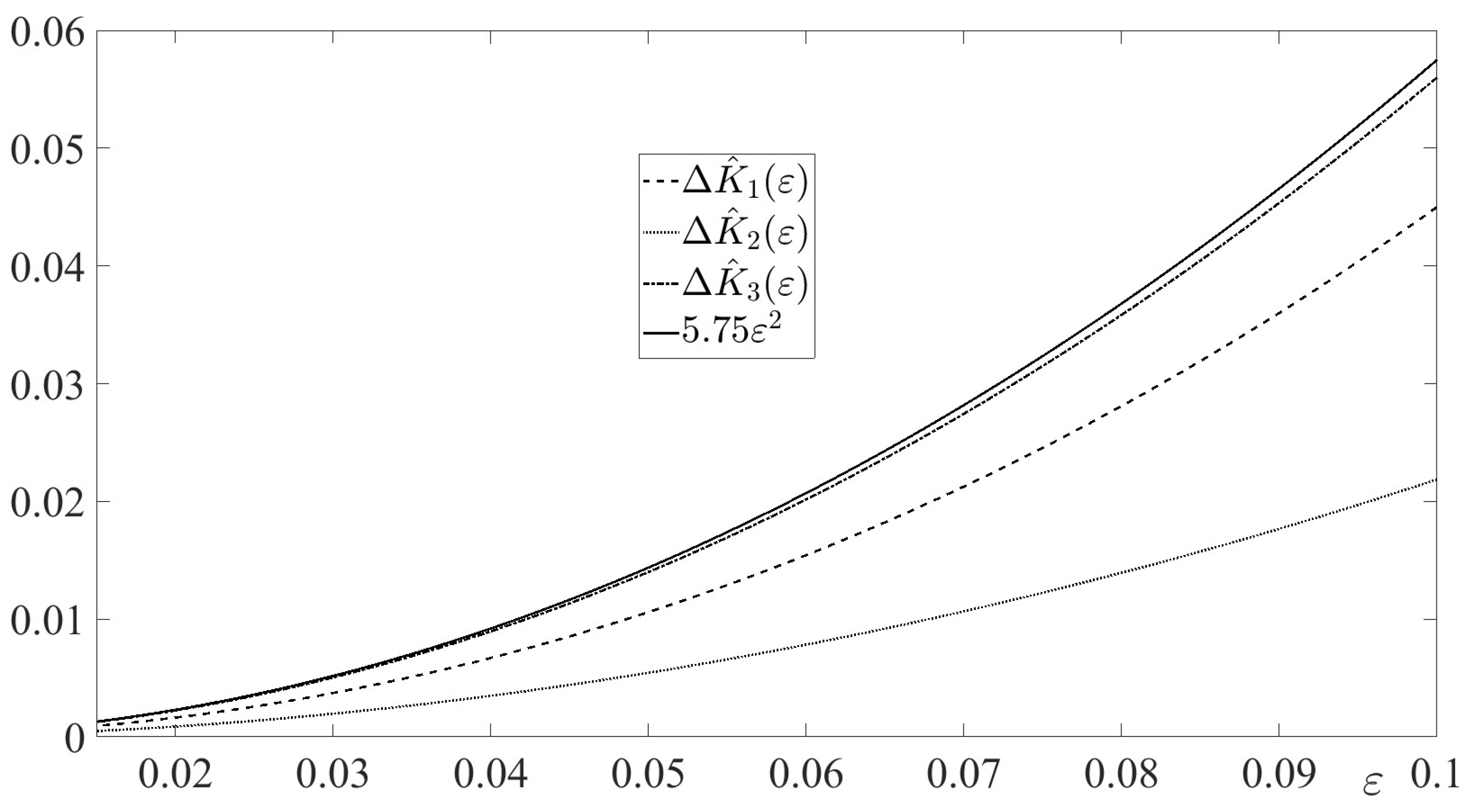
Figure 5.
Absolute errors and .
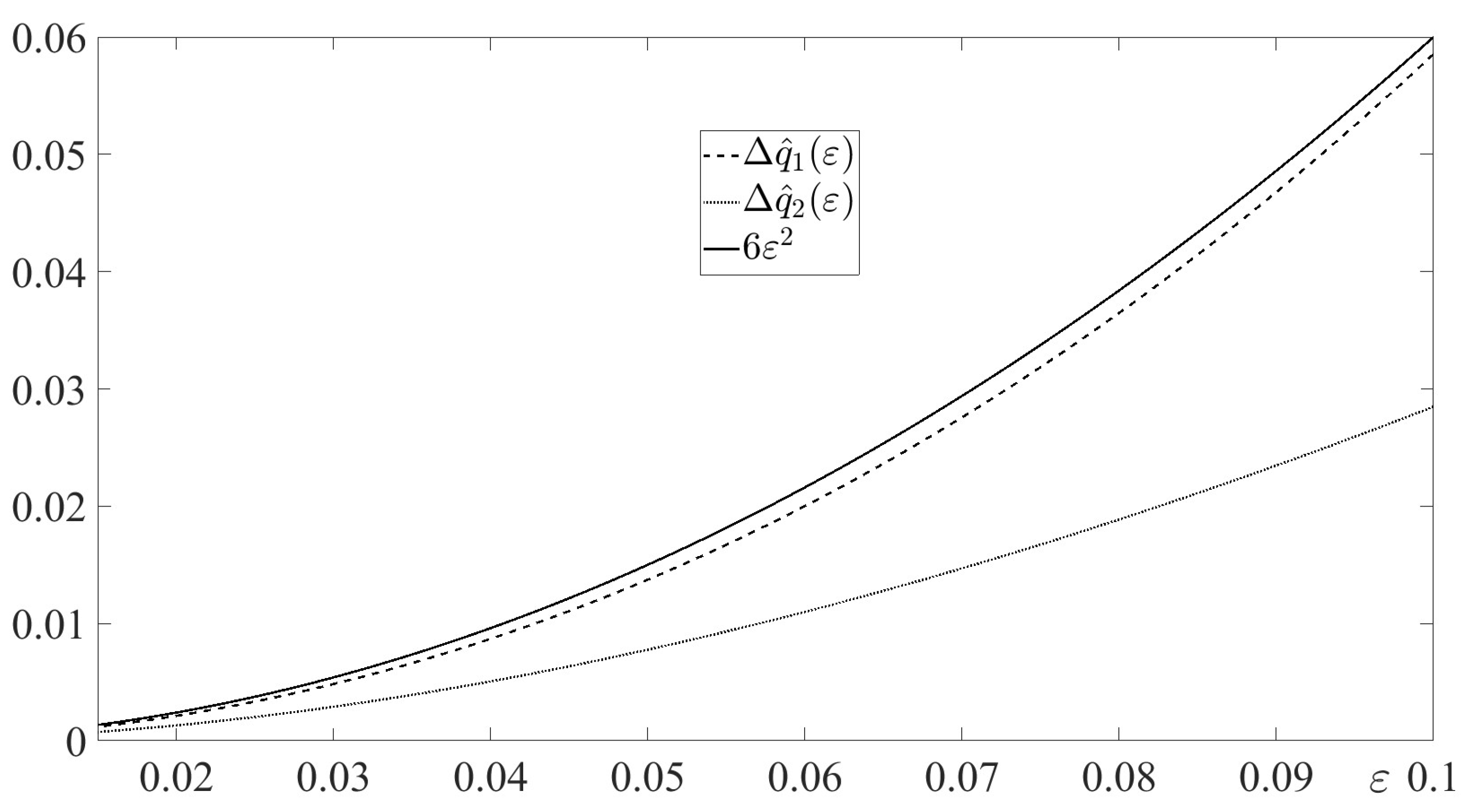
Figure 6.
Absolute error of the asymptotic expansion of .
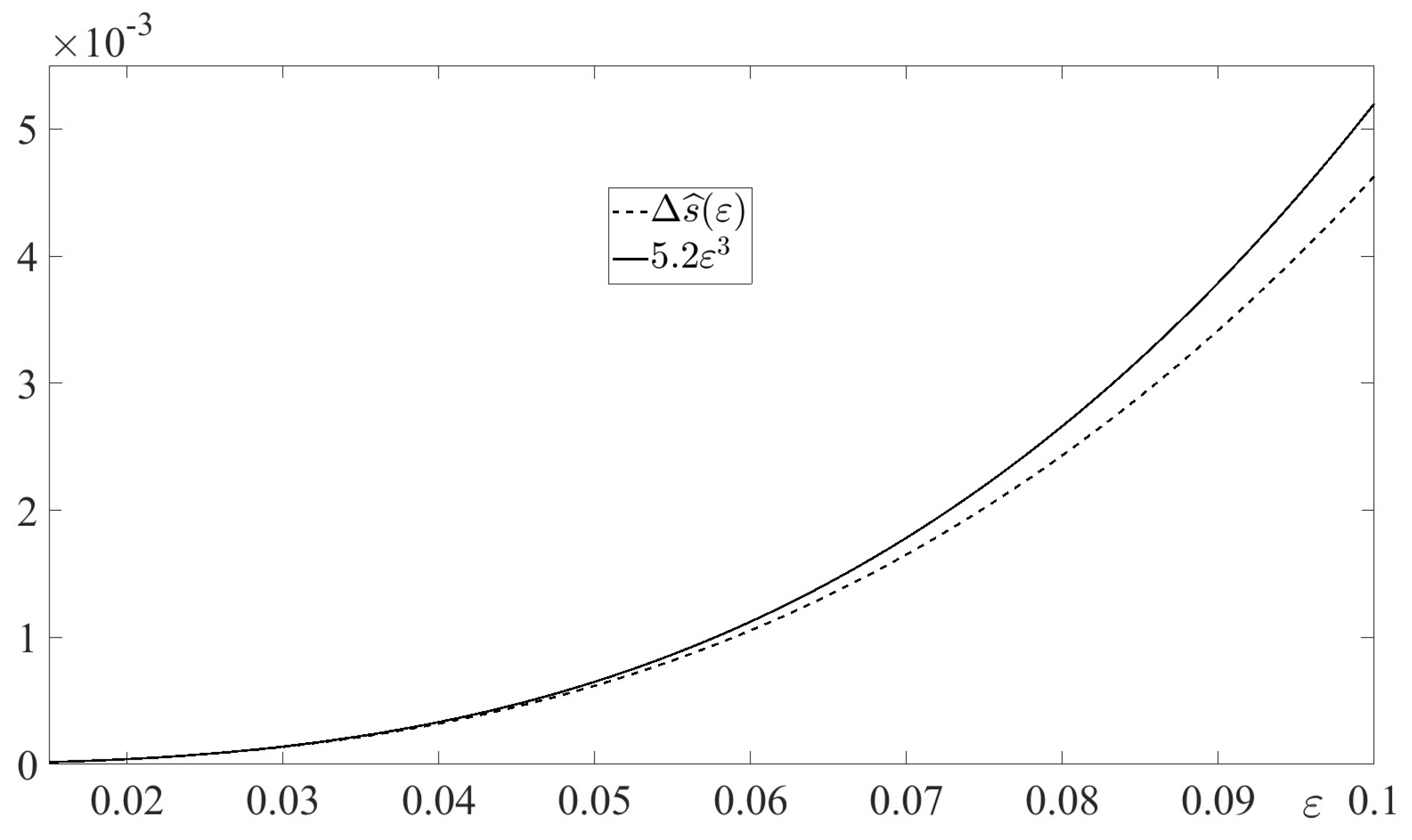

Table 1.
Values of , , , and in the Case I.
Table 2.
Absolute and relative errors of approximations in the Case I.
Table 3.
Values of , , , and in the Case II.
Table 4.
Absolute and relative errors of in the Case II.
Disclaimer/Publisher’s Note: The statements, opinions and data contained in all publications are solely those of the individual author(s) and contributor(s) and not of MDPI and/or the editor(s). MDPI and/or the editor(s) disclaim responsibility for any injury to people or property resulting from any ideas, methods, instructions or products referred to in the content. |
© 2025 by the authors. Licensee MDPI, Basel, Switzerland. This article is an open access article distributed under the terms and conditions of the Creative Commons Attribution (CC BY) license (http://creativecommons.org/licenses/by/4.0/).
Copyright: This open access article is published under a Creative Commons CC BY 4.0 license, which permit the free download, distribution, and reuse, provided that the author and preprint are cited in any reuse.


