Linear Quadratic Pursuit–Evasion Games on Time Scales

1. Introduction

The theory of deterministic pursuit-evasion games can single-handedly be attributed to Isaacs in the 1950s [1,2]. Here, Isaacs first considered differential games as two-player zero-sum games. One early application was formulation of missile guidance systems during his time with the RAND Corporation. Shortly thereafter, Kalman among others initiated the linear quadratic regulator and tracking (LQR) and (LQT) in the continuous and discrete cases (see [3,4,5,6]). Since then, the concept of pursuit-evasion games and optimal control have been closely related, each playing a fundamental role in control engineering and economics. One breakout paper to combine these concepts was written by Ho, Bryson, and Baron. Together, they studied linear quadratic pursuit-evasion games (LQPEG) as regulator problems [7,8]. In particular, this work included a three-dimensional target interception problem. Since then, there have been a number of papers that have extended these results in the continuous and discrete cases. One of the issues that researchers have faced in the past is the discrete nature of these mixed strategies.

In 1988, Stefan Hilger initiated the theory of dynamic equations of time scales, which seeks to unify and extend discrete and continuous analysis [9]. As a result, we can generalize a process to account for both cases, or any combination of the two provided we restrict ourselves to closed, nonempty subsets of the reals (a time scale). From a numerical viewpoint, this theory can be thought of a generalized sampling technique that allows a researcher to evaluate processes with continuous, discrete, or uneven measurements. Since its inception, this area of mathematics has gained a great deal of international attention. Researchers have since found applications of time scales to include heat transfer, population dynamics, as well as economics. For a more in depth study of time scales, it is suggested that one see Bohner and Peterson’s books [10,11].

There have been a number of researchers who have sought to combine this field with the theory of control. A number of authors have contributed to generalizing the basic notions of controllability and observability (see [12,13,14,15,16]). Bohner first provided the conditions for optimality for dynamic control processes in [17]. DaCunha unified the theory of Lyapunov and Floquet theory in his dissertation [18]. Hilscher along with Zeidan have studied optimal control for sympletic systems [19]. Additional contributions can be found in [20,21,22,23,24,25], among several others.

In this paper, we study a natural extension of the LQR and LQT previously generalized to dynamics equations on time scales (see [26,27]). Here, we consider the following separable dynamic systems

$$\begin{array}{ccc}\hfill x_P^{\Delta }\left(t\right)& =& A_P{x}_P\left(t\right)+B_{P}u\left(t\right),x_P\left(t_0\right)=x_0^P\hfill \\ \hfill x_E^{\Delta }\left(t\right)& =& A_E{x}_E\left(t\right)+B_{E}v\left(t\right),x_E\left(t_0\right)=x_0^E,\hfill \end{array}$$

(1.1)

where $x_i\in {\mathbb{R}}^n$ represent our states and $u,v\in {\mathbb{R}}^m$ represent our controls. Note that the subscripts P and E to stand for the pursuer and the evader respectively. The pursuing state seeks to intercept the evading state at time $t_{\mathrm{f}}$ while the latter state seeks to do the opposite. For simplicity, we make the following assumptions. First, we assume the given systems are linear-time invariant (although the strategies for the time-varying case can be determined in a similar fashion). Second, we assume that both states are controllable and are being evaluated on the same time scale. Finally, we assume our state equations are associated with the cost functional

$$\begin{array}{cc}\hfill J(u,v)=& {\displaystyle \frac{1}{2}}\left|\right|x_P-x_E{\left|\right|}_M\left(t_{\mathrm{f}}\right)+{\displaystyle \frac{1}{2}}{\int }_{t_0}^{t_{\mathrm{f}}}\left(\right||x_P-x_E{\left|\right|}_Q+{\left|\right|u\left|\right|}_{R_P}-{\left|\right|v\left|\right|}_{R_E})\left(\tau \right)\Delta \tau \hfill \\ \hfill =& {\displaystyle \frac{1}{2}}\left({(x_P-x_E)}^T\left(t_{\mathrm{f}}\right)M(x_P-x_E)\right)\left(t_{\mathrm{f}}\right)\hfill \\ & +{\displaystyle \frac{1}{2}}{\int }_{t_0}^{t_{\mathrm{f}}}\left({(x_P-x_E)}^{T}Q(x_P-x_E)+u^T{R}_{P}u-v^T{R}_{E}v\right)\left(\tau \right)\Delta \tau ,\hfill \end{array}$$

(1.2)

where $M\ge 0$ and diagonal, $Q\ge 0$ and $R_P$, $R_E>0$. Note that the goal of the pursuing state is to minimize (1.2) while the evading state seeks to maximize it. Since these states represent opposing players, evaluating this cost can be thought of as a minimax problem.

The pursuit-evasion framework remains an active area across multiple disciplines, as found in [28,29,30,31,32,33,34]. It should be noted that there have been other excursions in combining dynamic games with time scales calculus. Libich and Stehlík introduced macroeconomic policy games on times scales with inefficient equilibria in [35]. Martins and Torres considered $n-$player games where each player sought to minimize a shared cost functional. Mozhegova and Petrov introduced a simple pursuit problem in [36] and a dynamic analogue to the “Cossacks-robbers” in [37]. Minh and Phuong have previously studied linear pursuit-evasion games on time scales in [38]. However, these results do include a regulator/saddle point framework, nor are they complete when compared to this manuscript.

The organization of this paper is as follows. Section 2 presents core definitions and concepts of the time scales calculus. We offer the variational properties needed such that an optimal strategy exists in Section 3. In Section 4, we seek a mixed strategy when the final states are both fixed. In this setting, we can rewrite our cost functional (1.2) in terms of the difference in Gramians of each system. For Section 5, we find a pair of a controls in terms of an extended state. In Section 6, we offer some examples including a numerical result. Finally, we provide some concluding remarks and future plans in Section 7.

2. Time Scales Preliminaries

Here we offer a brief introduction to the theory of dynamic equations on time scales. For a more in-depth study of time scales, see Bohner and Peterson’s books [10,11].

Definition 1.

A time scale $\mathbb{T}$ is an arbitrary nonempty closed subset of the real numbers. We let ${\mathbb{T}}^{\kappa }=\mathbb{T}\setminus \{max\mathbb{T}\}$ if $max\mathbb{T}$ exists; otherwise ${\mathbb{T}}^{\kappa }=\mathbb{T}$.

Example 2.

The most common examples of time scales are $\mathbb{T}=\mathbb{R}$, $\mathbb{T}=\mathbb{Z}$, $\mathbb{T}=h\mathbb{Z}$ for $h>0$, and $\mathbb{T}=q^{{\mathbb{N}}_0}$ for $q>1$.

Definition 3.

We define the forward jump operator $\sigma :\mathbb{T}\to \mathbb{T}$ and the graininess function $\mu :\mathbb{T}\to [0,\infty )$ by

$$\sigma \left(t\right):=inf\left\{s\in \mathbb{T}:s>t\right\}\mathrm{a}\mathrm{n}\mathrm{d}\mu \left(t\right)=\sigma \left(t\right)-t.$$

Definition 4.

For any function $f:\mathbb{T}\to \mathbb{R}$, we define the function $f^{\sigma }:\mathbb{T}\to \mathbb{R}$ by $f^{\sigma }=f\circ \sigma$.

Next, we define the delta (or Hilger) derivative as follows.

Definition 5.

Assume $f:\mathbb{T}\to \mathbb{R}$ and let $t\in {\mathbb{T}}^{\kappa }$. The delta derivative $f^{\Delta }\left(t\right)$ is the number (when it exists) such that given any $\epsilon >0$, there is a neighborhood U of t such that

$$\left|[f\left(\sigma \left(t\right)\right)-f\left(s\right)]-f^{\Delta }\left(t\right)[\sigma \left(t\right)-s]\right|\le \epsilon |\sigma \left(t\right)-s|\mathrm{for}\mathrm{all}s\in U.$$

In the next two theorems, we consider some properties of the delta derivative.

Theorem 6

(See Theorem 1.16 [10]). Suppose $f:\mathbb{T}\to \mathbb{R}$ is a function and let $t\in {\mathbb{T}}^{\kappa }$. Then we have the following:

a. 

If f is differentiable at t, then f is continuous at t.

b. 

If f is continuous at t, where t is right-scattered, then f is differentiable at t and

$$f^{\Delta }\left(t\right)={\displaystyle \frac{f\left(\sigma \right(t\left)\right)-f\left(t\right)}{\mu \left(t\right)}}.$$

c. 

If f is differentiable at t, where t is right-dense, then

$$f^{\Delta }\left(t\right)=\underset{s\to t}{lim}{\displaystyle \frac{f\left(t\right)-f\left(s\right)}{t-s}}.$$

d. 

If f is differentiable at t, then

$$f\left(\sigma \left(t\right)\right)=f\left(t\right)+\mu \left(t\right)f^{\Delta }\left(t\right).$$

(2.1)

Note that (2.1) is sometimes called the “simple useful formula."

Example 7.

Note the following examples.

a.

When $\mathbb{T}=\mathbb{R}$, then (if the limit exists)

$$f^{\Delta }\left(t\right)=\underset{s\to t}{lim}{\displaystyle \frac{f\left(t\right)-f\left(s\right)}{t-s}}=f^{\prime }\left(t\right).$$

b.

When $\mathbb{T}=\mathbb{Z}$, then

$$f^{\Delta }\left(t\right)=f(t+1)-f\left(t\right)=:\Delta f\left(t\right).$$

c.

When $\mathbb{T}=h\mathbb{Z}$ for $h>0$, then

$$f^{\Delta }\left(t\right)={\displaystyle \frac{f(t+h)-f\left(t\right)}{h}}=:{\Delta }_{h}f\left(t\right).$$

d.

When $\mathbb{T}=q^{\mathbb{Z}}$ for $q>1$, then

$$f^{\Delta }\left(t\right)={\displaystyle \frac{f\left(qt\right)-f\left(t\right)}{(q-1)t}}=:D_{q}f\left(t\right).$$

Next we consider the linearity property as well as the product rules.

Theorem 8

(See Theorem 1.20 [10]). Let $f,g:\mathbb{T}\to \mathbb{R}$ be differentiable at $t\in {\mathbb{T}}^{\kappa }$. Then we have the following:

a. 

For any constants α and β, the sum $(\alpha f+\beta g):\mathbb{T}\to \mathbb{R}$ is differentiable at t with

$${(\alpha f+\beta g)}^{\Delta }\left(t\right)=\alpha f^{\Delta }\left(t\right)+\beta g^{\Delta }\left(t\right).$$

b. 

The product $fg:\mathbb{T}\to \mathbb{R}$ is differentiable at t with

$${\left(fg\right)}^{\Delta }\left(t\right)=f^{\Delta }\left(t\right)g\left(t\right)+f^{\sigma }\left(t\right)g^{\Delta }\left(t\right)=f\left(t\right)g^{\Delta }\left(t\right)+f^{\Delta }\left(t\right)g^{\sigma }\left(t\right).$$

Definition 9.

A function $f:\mathbb{T}\to \mathbb{R}$ is said to be rd-continuous on $\mathbb{T}$ when f is continuous in points $t\in \mathbb{T}$ with $\sigma \left(t\right)=t$ and it has finite left-sided limits in points $t\in \mathbb{T}$ with $sup\left\{s\in \mathbb{T}:s<t\right\}=t$. The class of rd-continuous functions $f:\mathbb{T}\to \mathbb{R}$ is denoted by ${\mathrm{C}}_{\mathrm{rd}}={\mathrm{C}}_{\mathrm{rd}}\left(\mathbb{T}\right)={\mathrm{C}}_{\mathrm{rd}}(\mathbb{T},\mathbb{R})$. The set of functions $f:\mathbb{T}\to \mathbb{R}$ that are differentiable and whose derivative is rd-continuous is denoted by ${\mathrm{C}}_{\mathrm{rd}}^1$.

Theorem 10

(See Theorem 1.74[10]). Any rd-continuous function $f:\mathbb{T}\to \mathbb{R}$ has an antiderivative F, i.e., $F^{\Delta }=f$ on ${\mathbb{T}}^{\kappa }$.

Definition 11.

Let $f\in {\mathrm{C}}_{\mathrm{rd}}$ and let F be any function such that $F^{\Delta }\left(t\right)=f\left(t\right)$ for all $t\in {\mathbb{T}}^{\kappa }$. Then the Cauchy integral of f is defined by

$${\int }_a^{b}f\left(t\right)\Delta t=F\left(b\right)-F\left(a\right)\mathrm{for} \mathrm{all}a,b\in \mathbb{T}.$$

Example 12.

Let $a,b\in \mathbb{T}$ with $a<b$ and assume that $f\in {\mathrm{C}}_{\mathrm{rd}}$.

a.

When $\mathbb{T}=\mathbb{R}$, then

$${\int }_a^{b}f\left(t\right)\Delta t={\int }_a^{b}f\left(t\right)\mathrm{d}t.$$

b.

When $\mathbb{T}=\mathbb{Z}$, then

$${\int }_a^{b}f\left(t\right)\Delta t=\sum _{t=a}^{b-1}f\left(t\right).$$

c.

When $\mathbb{T}=h\mathbb{Z}$ for $h>0$, then

$${\int }_a^{b}f\left(t\right)\Delta t=h\sum _{t=a/h}^{b/h-1}f\left(th\right).$$

d.

When $\mathbb{T}=q^{{\mathbb{N}}_0}$ for $q>1$, then

$${\int }_a^{b}f\left(t\right)\Delta t={\int }_a^{b}f\left(t\right){\mathrm{d}}_q\left(t\right):=(q-1)\sum _{t\in [a,b)\cap \mathbb{T}}tf\left(t\right).$$

Next, we present the matrix exponential and some of its properties.

Definition 13.

An $m\times n$ matrix-valued function A on $\mathbb{T}$ is rd-continuous if each of its entries are rd-continuous. Furthermore, if $m=n$, A is said to be regressive (we write $A\in \mathcal{R}$) if

$$I+\mu \left(t\right)A\left(t\right)\mathrm{is} \mathrm{invertible} \mathrm{for} \mathrm{all}t\in {\mathbb{T}}^{\kappa }.$$

Theorem 14

(See Theorem 5.8 [10]). Suppose that A is regressive and rd-continuous. Then the initial value problem

$$X^{\Delta }\left(t\right)=A\left(t\right)X\left(t\right),X\left(t_0\right)=I,$$

where I is the identity matrix, has a unique $n\times n$ matrix-valued solution X.

Definition 15.

The solution X from Theorem 14 is called the matrix exponential function on $\mathbb{T}$ and is denoted by $e_A(·,t_0)$.

Theorem 16

(See Theorem 5.21 [10]). Let A be regressive and rd-continuous. Then for $r,s,t\in \mathbb{T}$,

a. 

$e_A(t,s)e_A(s,r)=e_A(t,r)$, hence $e_A(t,t)=I$,

b. 

$e_A(\sigma \left(t\right),s)=(I+\mu \left(t\right)A\left(t\right))e_A(t,s)$,

c. 

$e_A(t,\sigma \left(s\right))=e_A(t,s){(I+\mu \left(s\right)A\left(s\right))}^{-1}$,

d. 

${\left(e_A(·,s)\right)}^{\Delta }=A{e}_A(·,s)$,

e. 

${\left(e_A(t,·)\right)}^{\Delta }=-e_A^{\sigma }(t,·)A\left(s\right)=-e_A(t,·){(I+\mu \left(s\right)A\left(s\right))}^{-1}A\left(s\right)$.

Next we give the solution (state response) to our linear system using variation of parameters.

Theorem 17

(See Theorem 5.24 [10]). Let $A\in \mathcal{R}$ be an $n\times n$ matrix-valued function on $\mathbb{T}$ and suppose that $f:\mathbb{T}\to {\mathbb{R}}^n$ is rd-continuous. Let $t_0\in \mathbb{T}$ and $x_0\in {\mathbb{R}}^n$. Then the solution of the initial value problem

$$x^{\Delta }\left(t\right)=A\left(t\right)x\left(t\right)+f\left(t\right),x\left(t_0\right)=x_0$$

is given by

$$x\left(t\right)=e_A(t,t_0)x_0+{\int }_{t_0}^t{e}_A(t,\sigma \left(\tau \right))f\left(\tau \right)\Delta \tau .$$

3. Optimization of Linear Systems on Time Scales

In this section, we make use of variational methods on time scales as introduced by Bohner in [17]. First, note that the state equations in (1.1) are uncoupled. For convenience, we rewrite (1.1) as

$$z^{\Delta }\left(t\right)=\widehat{A}z\left(t\right)+\widehat{B}u\left(t\right)+\widehat{C}v\left(t\right),z\left(t_0\right)=z_0,$$

(3.1)

where z represents an extended state given by $z={\left[\begin{array}{cc}{x}_P& x_E\end{array}\right]}^T$, $\widehat{A}=\left[\begin{array}{cc}{A}_P& 0\\ 0& A_E\end{array}\right]$, $\widehat{B}={\left[\begin{array}{cc}{B}_P& 0\end{array}\right]}^T$, and $\widehat{C}={\left[\begin{array}{cc}0& B_E\end{array}\right]}^T$. Associated with (3.1) is the quadratic cost functional

$$J(u,v)={\displaystyle \frac{1}{2}}{z}^T\left(t_{\mathrm{f}}\right)\widehat{M}z\left(t_{\mathrm{f}}\right)+{\displaystyle \frac{1}{2}}{\int }_{t_0}^{t_{\mathrm{f}}}(z^T\widehat{Q}z+u^T{R}_{P}u-v^T{R}_{E}v)\left(\tau \right)\Delta \tau ,$$

(3.2)

where $\widehat{M}$, $\widehat{Q}\ge 0$ and $R_P$, $R_E>0$. To minimize (3.2), we introduce the augmented cost functional

$$J^{+}(u,v)={\displaystyle \frac{1}{2}}{z}^T\left(t_{\mathrm{f}}\right)\widehat{M}z\left(t_{\mathrm{f}}\right)+{\int }_{t_0}^{t_{\mathrm{f}}}[H(x,u,v,{\lambda }^{\sigma })-{\left({\lambda }^{\sigma }\right)}^T{z}^{\Delta }]\left(\tau \right)\Delta \tau ,$$

where the so-called Hamiltonian H is given by

$$H(x,u,v,\lambda )={\displaystyle \frac{1}{2}}(z^T\widehat{Q}z+u^T{R}_{P}u-v^T{R}_{E}v)+{\lambda }^T(\widehat{A}z+\widehat{B}u+\widehat{C}v)$$

(3.3)

and $\lambda ={\left[\begin{array}{cc}{\lambda }_P& {\lambda }_E\end{array}\right]}^T$ represents a multiplier to be determined later.

Remark 18.

Our treatment of (1.1) differs from the argument used by Ho, Bryson, and Baron in [7]. In their paper, they appealed to state estimates of the pursuer and evader to evaluate the cost functional. Their motivation for their argument is due to notion that when they studied pursing and evading missiles, they considered difference in altitude as negligible. As a result of our rewriting of (1.1), we are not required to make such a restriction.

Next, we provide necessary conditions for an optimal control. We assume that

$${\displaystyle \frac{\mathrm{d}}{\mathrm{d}\epsilon }}{\int }_{t_0}^{t_{\mathrm{f}}}f(\tau ,\epsilon )\Delta \tau ={\int }_{t_0}^{t_{\mathrm{f}}}{\displaystyle \frac{\partial }{\partial \epsilon }}f(\tau ,\epsilon )\Delta \tau$$

(3.4)

for all $f:\mathbb{T}\times \mathbb{R}\to \mathbb{R}$ such that $f(·,\epsilon ),\partial f(·,\epsilon )/\partial \epsilon \in {\mathrm{C}}_{\mathrm{rd}}\left(\mathbb{T}\right)$.

Lemma 19.

Let (3.2) be the cost functional associated with (3.1). Assume (3.4) holds. Then the first variation, $\dot{\Phi }\left(0\right)$, is zero provided that z, λ, u, and v satisfy

$$\begin{array}{c}{z}^{\Delta }=\widehat{A}z+\widehat{B}u+\widehat{C}v,\end{array}$$

(3.5a)

$$\begin{array}{c}-{\lambda }^{\Delta }=\widehat{Q}z+{\widehat{A}}^T{\lambda }^{\sigma },\end{array}$$

(3.5b)

$$\begin{array}{c}0=R_{P}u+{\widehat{B}}^T{\lambda }^{\sigma },\end{array}$$

(3.5c)

$$\begin{array}{c}0=-R_{E}v+{\widehat{C}}^T{\lambda }^{\sigma }.\end{array}$$

(3.5d)

Proof. 

First note that

$$\begin{array}{cc}\Phi \left(\epsilon \right)=& {\displaystyle \mathcal{J}((z,u,v,\lambda )+\epsilon ({\eta }_1,{\eta }_2,{\eta }_3,{\eta }_4))}\hfill \\ =& {\displaystyle \frac{1}{2}}{(z+\epsilon {\eta }_1)}^T\left(t_{\mathrm{f}}\right)\widehat{M}(z+\epsilon {\eta }_1)\left(t_{\mathrm{f}}\right)+{\displaystyle \frac{1}{2}}{\int }_{t_0}^{t_{\mathrm{f}}}\left[{(z+\epsilon {\eta }_1)}^T\widehat{Q}(z+\epsilon {\eta }_1)\right]\left(\tau \right)\Delta \tau \hfill \\ & +{\displaystyle \frac{1}{2}}{\int }_{t_0}^{t_{\mathrm{f}}}\left[{(u+\epsilon {\eta }_2)}^T{R}_P(u+\epsilon {\eta }_2)\right]\left(\tau \right)\Delta \tau -{\displaystyle \frac{1}{2}}{\int }_{t_0}^{t_{\mathrm{f}}}\left[{(v+\epsilon {\eta }_3)}^T{R}_E(v+\epsilon {\eta }_3)\right]\left(\tau \right)\Delta \tau \hfill \\ & +{\int }_{t_0}^{t_{\mathrm{f}}}\left\{{({\lambda }^{\sigma }+\epsilon {\eta }_4^{\sigma })}^T[\widehat{A}(z+\epsilon {\eta }_1)+\widehat{B}(u+\epsilon {\eta }_2)\right\}\left(\tau \right)\Delta \tau \hfill \\ & +{\int }_{t_0}^{t_{\mathrm{f}}}\left\{{({\lambda }^{\sigma }+\epsilon {\eta }_4^{\sigma })}^T[\widehat{C}(v+\epsilon {\eta }_3)-{(z+\epsilon {\eta }_1)}^{\Delta }]\right\}\left(\tau \right)\Delta \tau .\hfill \end{array}$$

Then

$$\begin{array}{cc}\dot{\Phi }\left(\epsilon \right)& {\displaystyle ={\eta }_1^T\left(t_{\mathrm{f}}\right)\widehat{M}(z+\epsilon {\eta }_1)\left(t_{\mathrm{f}}\right)+{\int }_{t_0}^{t_{\mathrm{f}}}\left[{\eta }_1^T\widehat{Q}(z+\epsilon {\eta }_1)\right]\left(\tau \right)\Delta \tau }\hfill \\ & +{\int }_{t_0}^{t_{\mathrm{f}}}[{\eta }_2^T{R}_P(u+\epsilon {\eta }_2)-{\eta }_3^T{R}_E(v+\epsilon {\eta }_3)]\left(\tau \right)\Delta \tau \hfill \\ & +{\int }_{t_0}^{t_{\mathrm{f}}}\left\{{\left({\eta }_4^{\sigma }\right)}^T[\widehat{A}(z+\epsilon {\eta }_1)+\widehat{B}(u+\epsilon {\eta }_2)]\right\}\left(\tau \right)\Delta \tau \hfill \\ & +{\int }_{t_0}^{t_{\mathrm{f}}}\left\{{\left({\eta }_4^{\sigma }\right)}^T[\widehat{C}(v+\epsilon {\eta }_3)-{(z+\epsilon {\eta }_1)}^{\Delta }]\right\}\left(\tau \right)\Delta \tau \hfill \\ & +{\int }_{t_0}^{t_{\mathrm{f}}}\left\{{({\lambda }^{\sigma }+\epsilon {\eta }_4^{\sigma })}^T[\widehat{A}{\eta }_1+\widehat{B}{\eta }_2+\widehat{C}{\eta }_3-{\eta }_1^{\Delta }]\right\}\left(\tau \right)\Delta \tau .\hfill \end{array}$$

Then after rearranging terms, the first variation can be written as

$$\begin{array}{cc}\hfill \dot{\Phi }\left(0\right)& {\displaystyle ={[\widehat{M}z\left(t_{\mathrm{f}}\right)-\lambda \left(t_{\mathrm{f}}\right)]}^T{\eta }_1\left(t_{\mathrm{f}}\right)+{\lambda }^T\left(t_0\right){\eta }_1\left(t_0\right)}\hfill \\ & +{\int }_{t_0}^{t_{\mathrm{f}}}[{({\widehat{A}}^T{\lambda }^{\sigma }+\widehat{Q}z+{\lambda }^{\Delta })}^T{\eta }_1+{(R_{P}u+{\widehat{B}}^T{\lambda }^{\sigma })}^T{\eta }_2]\left(\tau \right)\Delta \tau \hfill \\ & +{\int }_{t_0}^{t_{\mathrm{f}}}[{(-R_{E}v+{\widehat{C}}^T{\lambda }^{\sigma })}^T{\eta }_3+{(\widehat{A}z+\widehat{B}u+\widehat{C}v-z^{\Delta })}^T{\eta }_4^{\sigma }]\left(\tau \right)\Delta \tau .\hfill \end{array}$$

Now in order for $\dot{\Phi }\left(0\right)=0$, we set each coefficient of independent increments ${\eta }_1$, ${\eta }_2$, ${\eta }_3$, ${\eta }_4^{\sigma }$ equal to zero. This yields the necessary conditions for a minimum of (3.2). Using the Hamiltonian (3.3), we have state and costate equations

$$z^{\Delta }=H_{\lambda }(z,u,v,{\lambda }^{\sigma })=\widehat{A}z+\widehat{B}u+\widehat{C}v$$

and

$$-{\lambda }^{\Delta }=H_z(z,u,v,{\lambda }^{\sigma })=\widehat{Q}z+{\widehat{A}}^T{\lambda }^{\sigma }.$$

Similarly, we have the stationary conditions

$$0=H_u(z,u,v,{\lambda }^{\sigma })=R_{P}u+{\widehat{B}}^T{\lambda }^{\sigma }$$

and

$$0=H_v(z,u,v,{\lambda }^{\sigma })=-R_{E}v+{\widehat{C}}^T{\lambda }^{\sigma }$$

This concludes the proof. □

Remark 20.

We note that z, $\lambda$, u, and v solve (3.5) if and only if they solve

$$\begin{array}{c}{z}^{\Delta }=\widehat{A}z-\widehat{D}{\lambda }^{\sigma },\end{array}$$

(3.6a)

$$\begin{array}{c}-{\lambda }^{\Delta }=\widehat{Q}z+{\widehat{A}}^T{\lambda }^{\sigma },\end{array}$$

(3.6b)

$$\begin{array}{c}u=-R_P^{-1}{\widehat{B}}^T{\lambda }^{\sigma },\end{array}$$

(3.6c)

$$\begin{array}{c}v=R_E^{-1}{\widehat{C}}^T{\lambda }^{\sigma },\end{array}$$

(3.6d)

where $\widehat{D}$ is a “mixing term” given by

$$\widehat{D}:=\widehat{B}{R}_P^{-1}{\widehat{B}}^T-\widehat{C}{R}_E^{-1}{\widehat{C}}^T.$$

Throughout this paper, we assume that $\widehat{D}$ is regressive. As a result, we can determine an optimal strategy if we know the value of the costate.

Finally, we give the sufficient conditions for a local optimal control.

Lemma 21.

Let (3.2) be the cost functional associated with (3.1). Assume (3.4) holds. Then the second variation, $\ddot{\Phi }\left(0\right)$, is positive provided that ${\eta }_1$, ${\eta }_2$, and ${\eta }_3$ satisfy the constraints ${\eta }_1^{\Delta }=\widehat{A}{\eta }_1+\widehat{B}{\eta }_2+\widehat{C}{\eta }_3$ where ${\eta }_2\ne 0$ and ${\eta }_3$ is fixed.

Proof. 

Taking the second derivative of $\Phi \left(\epsilon \right)$, we have

$$\begin{array}{ccc}\hfill \ddot{\Phi }\left(\epsilon \right)& =& {\eta }_1^T\left(t_{\mathrm{f}}\right)\widehat{M}{\eta }_1\left(t_{\mathrm{f}}\right)+{\int }_{t_0}^{t_{\mathrm{f}}}[{\eta }_1^T\widehat{Q}{\eta }_1+{\eta }_2^T{R}_P{\eta }_2-{\eta }_3^T{R}_E{\eta }_3]\left(\tau \right)\Delta \tau \hfill \\ & & +2{\int }_{t_0}^{t_{\mathrm{f}}}\left[{(\widehat{A}{\eta }_1+\widehat{B}{\eta }_2+\widehat{C}{\eta }_3-{\eta }_1^{\Delta })}^T{\eta }_4^{\sigma }\right]\left(\tau \right)\Delta \tau .\hfill \end{array}$$

If we assume that ${\eta }_1$, ${\eta }_2$, and ${\eta }_3$ satisfy the constraint

$${\eta }_1^{\Delta }=\widehat{A}{\eta }_1+\widehat{B}{\eta }_2+\widehat{C}{\eta }_3,$$

then the second variation is given by

$$\ddot{\Phi }\left(0\right)={\eta }_1^T\left(t_{\mathrm{f}}\right)\widehat{M}{\eta }_1\left(t_{\mathrm{f}}\right)+{\int }_{t_0}^{t_{\mathrm{f}}}[{\eta }_1^T\widehat{Q}{\eta }_1+{\eta }_2^T{R}_P{\eta }_2-{\eta }_3^T{R}_E{\eta }_3]\left(\tau \right)\Delta \tau .$$

Note that $\widehat{M}$ and $\widehat{Q}\ge 0$ while $R_P$ and $R_E>0$. Thus if ${\eta }_2\ne 0$ and ${\eta }_3$ is fixed, then (3.7) is guaranteed to be positive. □

Definition 22.

The pair $(u^{*},v^{*})$ is a saddle point to the system (3.1) associated with the cost (3.2) provided

$$J(u,v^{*})\le J(u^{*},v^{*})\le J(u^{*},v).$$

Here, the stationary conditions needed to ensure a saddle are $H_{uu}=R_P>0$ and $H_{vv}=-R_E<0$ (see [39]). For our purposes, this pair corresponds to when neither player wishes to deviate from this compromise without being penalized by the other player. It be understood that this compromise occurs when we have the natural caveat that the pursuer and evader belong to the same time scale. In this paper, we do not claim that this saddle point must be unique.

4. Fixed Final States Case

In this section, we seek an optimal strategy when the final states are fixed. In this setting we write the equations for the pursuer and evader separately. Here we consider the state and costate equations for the pursuer

$$\begin{array}{cccc}\hfill x_P^{\Delta }\left(t\right)& =& A_P{x}_P\left(t\right)-B_P{R}_P^{-1}{B}_P^T{\lambda }_P^{\sigma }\left(t\right),\hfill & x_P\left(t_0\right)=x_0^P\hfill \\ \hfill -{\lambda }_P^{\Delta }\left(t\right)& =& A_P^T{\lambda }_P^{\sigma }\left(t\right),\hfill & {\lambda }_P\left(t_{\mathrm{f}}\right)=M(x_P-x_E)\left(t_{\mathrm{f}}\right)\hfill \end{array}$$

(4.1)

as well as those for the evader

$$\begin{array}{cccc}\hfill x_E^{\Delta }\left(t\right)& =& A_E{x}_E\left(t\right)-B_E{R}_E^{-1}{B}_E^T{\lambda }_E^{\sigma }\left(t\right),\hfill & x_E\left(t_0\right)=x_0^E\hfill \\ \hfill -{\lambda }_E^{\Delta }\left(t\right)& =& A_E^T{\lambda }_E^{\sigma }\left(t\right),\hfill & {\lambda }_E\left(t_{\mathrm{f}}\right)=M(x_E-x_P)\left(t_{\mathrm{f}}\right)\hfill \end{array}$$

(4.2)

associated with the cost functional

$$\begin{array}{cc}\hfill J(u,v)& ={\displaystyle \frac{1}{2}}\left({(x_P-x_E)}^T\left(t_{\mathrm{f}}\right)M(x_P-x_E)\right)\left(t_{\mathrm{f}}\right)\hfill \\ & +{\displaystyle \frac{1}{2}}{\int }_{t_0}^{t_{\mathrm{f}}}\left({(x_P-x_E)}^{T}Q(x_P-x_E)+u^T{R}_{P}u-v^T{R}_{E}v\right)\left(\tau \right)\Delta \tau .\hfill \end{array}$$

(4.3)

Definition 23.

The initial state difference, $d_0(·)$, is the difference between the zero-input pursuing and evading states, i.e.,

$$d_0\left(t\right):=e_{A_P}(t,t_0)x_P\left(t_0\right)-e_{A_E}(t,t_0)x_E\left(t_0\right).$$

Next, we determine an open–loop strategy for both players. Note that the following theorem mirrors Kalman’s generalized controllability criterion as found in Theorem 3.2 [16].

Theorem 24.

Suppose that $x_P$ and ${\lambda }_P$ solve (4.1) while $x_E$ and ${\lambda }_E$ satisfy (4.2). Let the Gramians for the pursuer and evader

$$G_P(t_o,t_{\mathrm{f}}):={\int }_{t_0}^{t_{\mathrm{f}}}{e}_{A_P}(t_{\mathrm{f}},\sigma \left(\tau \right))B_P{R}_P^{-1}{B}_P^T{e}_{A_P}^T(t_{\mathrm{f}},\sigma \left(\tau \right))\Delta \tau$$

(4.4)

and

$$G_E(t_o,t_{\mathrm{f}}):={\int }_{t_0}^{t_{\mathrm{f}}}{e}_{A_E}(t_{\mathrm{f}},\sigma \left(\tau \right))B_E{R}_E^{-1}{B}_E^T{e}_{A_E}^T(t_{\mathrm{f}},\sigma \left(\tau \right))\Delta \tau ,$$

(4.5)

respectively, be such that $I+(G_P-G_E)(t_0,t_{\mathrm{f}})M$ is invertible for all $t\in [t_0,t_{\mathrm{f}}]\cap \mathbb{T}$. Then u and v can be rewritten as

$$u\left(t\right)=-R_P^{-1}{B}_P^T{e}_{A_P}^T(t_{\mathrm{f}},\sigma \left(t\right))M{[I+(G_P-G_E)(t_o,t_{\mathrm{f}})M]}^{-1}{d}_0\left(t_{\mathrm{f}}\right)$$

(4.6)

and

$$v\left(t\right)=-R_E^{-1}{B}_E^T{e}_{A_E}^T(t_{\mathrm{f}},\sigma \left(t\right))M{[I+(G_P-G_E)(t_o,t_{\mathrm{f}})M]}^{-1}{d}_0\left(t_{\mathrm{f}}\right).$$

(4.7)

Proof. 

Solving (4.1) for ${\lambda }_P$, we have

$${\lambda }_P\left(t\right)=e_{A_P}^T(t_{\mathrm{f}},t){\lambda }_P\left(t_{\mathrm{f}}\right)=e_{A_P}^T(t_{\mathrm{f}},t)M(x_P-x_E)\left(t_{\mathrm{f}}\right).$$

Using (2.1) and (3.5a), the state equation becomes

$$x_P^{\Delta }\left(t\right)=A_P{x}_P\left(t\right)-B_P{R}_P^{-1}{B}_P^T{e}_{A_P}^T(t_{\mathrm{f}},\sigma \left(t\right)){\lambda }_P\left(t_{\mathrm{f}}\right).$$

(4.8)

Now solving (4.8) with Theorem 17 at time $t=t_{\mathrm{f}}$, we have

$$\begin{array}{cc}{x}_P\left(t_{\mathrm{f}}\right)& {\displaystyle =e_{A_P}(t_{\mathrm{f}},t_0)x_P\left(t_0\right)}\hfill \\ & -{\int }_{t_0}^{t_{\mathrm{f}}}{e}_{A_P}(t_{\mathrm{f}},\sigma \left(\tau \right))B_P{R}_P^{-1}{B}_P^T{e}_{A_P}^T(t_{\mathrm{f}},\sigma \left(\tau \right)){\lambda }_P\left(t_{\mathrm{f}}\right)\Delta \tau \hfill \\ =& e_{A_P}(t_{\mathrm{f}},t_0)x_P\left(t_0\right)-G_P(t_0,t_{\mathrm{f}})M(x_P-x_E)\left(t_{\mathrm{f}}\right).\hfill \end{array}$$

Similarly, the final state for the pursuer can be written as

$$x_E\left(t_{\mathrm{f}}\right)=e_{A_E}(t_{\mathrm{f}},t_0)x_E\left(t_0\right)-G_E(t_o,t_{\mathrm{f}})M(x_P-x_E)\left(t_{\mathrm{f}}\right).$$

Taking the difference in the final states and rearranging, we have

$$\begin{array}{ccc}\hfill (x_P-x_E)\left(t_{\mathrm{f}}\right)& =& d_0\left(t_{\mathrm{f}}\right)-(G_P-G_E)(t_0,t_{\mathrm{f}})M(x_P-x_E)\left(t_{\mathrm{f}}\right)\hfill \\ & =& {[I+(G_P-G_E)(t_0,t_{\mathrm{f}})M]}^{-1}{d}_0\left(t_{\mathrm{f}}\right).\hfill \end{array}$$

(4.9)

Finally, plugging $\lambda$ into (3.6c) and using (4.9) yields

$$\begin{array}{cc}u\left(t\right)=& {\displaystyle -R_P^{-1}{B}_P^T{e}_{A_P}^T(t_{\mathrm{f}},\sigma \left(t\right)){\lambda }_P\left(t_{\mathrm{f}}\right)}\hfill \\ =& -R_P^{-1}{B}_P^T{e}_{A_P}^T(t_{\mathrm{f}},\sigma \left(t\right))M(x_P-x_E)\left(t_{\mathrm{f}}\right)\hfill \\ =& -R_P^{-1}{B}_P^T{e}_{A_P}^T(t_{\mathrm{f}},\sigma \left(t\right))M{[I+(G_P-G_E)(t_o,t_{\mathrm{f}})M]}^{-1}{d}_0\left(t_{\mathrm{f}}\right).\hfill \end{array}$$

The equation for v can be shown similarly. This concludes the proof. □

Next, we determine the optimal cost.

Theorem 25.

If u and v are given by (4.6) and (4.7), respectively, then the cost functional (4.3) can be rewritten as

$$J(u,v)={\displaystyle \frac{1}{2}}{d}_0^T\left(t_{\mathrm{f}}\right)H(t_0,t_{\mathrm{f}})M^T[I+(G_P-G_E)(t_0,t_{\mathrm{f}})]MH(t_0,t_{\mathrm{f}})d_0\left(t_{\mathrm{f}}\right),$$

(4.10)

where $H(t_0,t_{\mathrm{f}}):={[I+(G_P-G_E)(t_0,t_{\mathrm{f}})M]}^{-1}$.

Proof. 

First, plugging (4.6), (4.7), and (4.9) into (4.3), we have

$$\begin{array}{cc}\hfill J(u,v)& ={\displaystyle \frac{1}{2}}{d}_0^T\left(t_{\mathrm{f}}\right)H(t_0,t_{\mathrm{f}})MH(t_0,t_{\mathrm{f}})d_0\left(t_{\mathrm{f}}\right)\hfill \\ & +{\displaystyle \frac{1}{2}}{d}_0^T\left(t_{\mathrm{f}}\right)H(t_0,t_{\mathrm{f}})M^T\left({\int }_{t_0}^{t_{\mathrm{f}}}{e}_{A_P}(t_{\mathrm{f}},\sigma \left(\tau \right))B_P{R}_P^{-1}{B}_P^T{e}_{A_P}^T(t_{\mathrm{f}},\sigma \left(\tau \right))\Delta \tau \right)MH(t_0,t_{\mathrm{f}})d_0\left(t_{\mathrm{f}}\right)\hfill \\ & -{\displaystyle \frac{1}{2}}{d}_0^T\left(t_{\mathrm{f}}\right)H(t_0,t_{\mathrm{f}})M^T\left({\int }_{t_0}^{t_{\mathrm{f}}}{e}_{A_E}(t_{\mathrm{f}},\sigma \left(\tau \right))B_E{R}_E^{-1}{B}_E^T{e}_{A_E}^T(t_{\mathrm{f}},\sigma \left(\tau \right))\Delta \tau \right)MH(t_0,t_{\mathrm{f}})d_0\left(t_{\mathrm{f}}\right)\hfill \\ & ={\displaystyle \frac{1}{2}}{d}_0^T\left(t_{\mathrm{f}}\right)H(t_0,t_{\mathrm{f}})MH(t_0,t_{\mathrm{f}})d_0\left(t_{\mathrm{f}}\right)\hfill \\ & +{\displaystyle \frac{1}{2}}{d}_0^T\left(t_{\mathrm{f}}\right)H(t_0,t_{\mathrm{f}})M^T(G_P-G_E)(t_0,t_{\mathrm{f}})]MH(t_0,t_{\mathrm{f}})d_0\left(t_{\mathrm{f}}\right),\hfill \end{array}$$

using the gramians (4.4) and (4.5). Since $M\ge 0$ is symmetric, we can pull out common factors on the left and right to obtain our result. □

Remark 26.

Suppose that the pursuer wants to use a strategy u that intercepts the evader (using strategy v) with minimal energy. Note that $det[I+(G_P-G_E)(t_0,t_{\mathrm{f}})]\ne 0$ if and only if $det\left[(G_P-G_E)(t_0,t_{\mathrm{f}})\right]\ne 0$. From the classical definition of controllability, this implies that the pursuer captures the evader when the pursuer is “more controllable" than the evader. A sufficient condition for the pursuing state to intercept the evader is given by $(G_P-G_E)(t_0,t_{\mathrm{f}})>0$. As a result, this relationship is preserved in the unification of pursuit-evasion to dynamic equations on time scales.

5. Free Final States Case

In this section, we develop an optimal control law in the form of state feedback. In considering the boundary conditions, note that $z\left(t_0\right)$ is known (meaning ${\eta }_1\left(t_0\right)=0$) while $z\left(t_{\mathrm{f}}\right)$ is free (meaning ${\eta }_1\left(t_{\mathrm{f}}\right)\ne 0$). Thus the coefficient on ${\eta }_1\left(t_{\mathrm{f}}\right)$ must be zero. This gives the terminal condition on the costate to be

$$\lambda \left(t_{\mathrm{f}}\right)=\widehat{M}z\left(t_{\mathrm{f}}\right).$$

(5.1)

Remark 27.

Now in order to solve this two-point boundary value problem, we make the assumption that z and $\lambda$ satisfy

$$\lambda \left(t\right)=S\left(t\right)z\left(t\right).$$

(5.2)

for all $t\in [t_0,t_{\mathrm{f}}]$. This condition (5.2) is called a “sweep condition," a term used by Bryson and Ho in [8]. Since the terminal condition $\widehat{M}\ge 0$, it is natural to assume that $S\ge 0$ as well.

Theorem 28.

Assume that S solves

$$-S^{\Delta }=\widehat{Q}+{\widehat{A}}^T{S}^{\sigma }+(I+\mu {\widehat{A}}^T)S^{\sigma }{(I+\mu \widehat{D}{S}^{\sigma })}^{-1}(\widehat{A}-\widehat{D}{S}^{\sigma }).$$

(5.3)

If x satisfies

$$z^{\Delta }={(I+\mu \widehat{D}{S}^{\sigma })}^{-1}(A-\widehat{D}{S}^{\sigma })z$$

(5.4)

and λ is given by (5.2), then

$$-{\lambda }^{\Delta }=\widehat{Q}z+{\widehat{A}}^T{\lambda }^{\sigma }.$$

(5.5)

Proof. 

Since $\lambda$ is as given in (5.2), we may use the product rule, (5.3), (5.4), and (2.1) to arrive at

$$\begin{array}{cc}-{\lambda }^{\Delta }=& {\displaystyle -S^{\Delta }z-S^{\sigma }{z}^{\Delta }}\hfill \\ =& \widehat{Q}z+{\widehat{A}}^T{S}^{\sigma }z+(I+\mu {\widehat{A}}^T)S^{\sigma }z-S^{\Delta }z\hfill \\ =& \widehat{Q}z+{\widehat{A}}^T{S}^{\sigma }z+\mu {\widehat{A}}^T{S}^{\sigma }{z}^{\Delta }\hfill \\ =& \widehat{Q}z+{\widehat{A}}^T{S}^{\sigma }{z}^{\sigma }\hfill \\ =& \widehat{Q}z+{\widehat{A}}^T{\lambda }^{\sigma },\hfill \end{array}$$

which gives (5.5) as desired. □

Next we offer an alternative form of our Riccati equation.

Lemma 29.

If $\widehat{D}{S}^{\sigma }$ is regressive, then S solves (5.3) if and only if it solves

$$-S^{\Delta }=\widehat{Q}+{\widehat{A}}^T{S}^{\sigma }+(I+\mu {\widehat{A}}^T)S^{\sigma }\widehat{A}-(I+\mu {\widehat{A}}^T)S^{\sigma }\widehat{D}{S}^{\sigma }{(I+\mu \widehat{D}{S}^{\sigma })}^{-1}(I+\mu \widehat{A}).$$

(5.6)

Proof. 

Note that

$$A-\widehat{D}{S}^{\sigma }=A-\widehat{D}{S}^{\sigma }(I+\mu A-\mu A)=(I+\mu \widehat{D}{S}^{\sigma })A-\widehat{D}{S}^{\sigma }(I+\mu A).$$

Plugging the above identity into (5.3) yields (5.6). □

Next we define our Kalman gains as follows.

Definition 30.

Let $\widehat{D}{S}^{\sigma }$ be regressive. Then the matrix-valued functions

$$K_P\left(t\right)=R_P^{-1}{\widehat{B}}^T{S}^{\sigma }\left(t\right){(I+\mu \left(t\right)\widehat{D}{S}^{\sigma }\left(t\right))}^{-1}(I+\mu \left(t\right)\widehat{A})$$

(5.7)

and

$$K_E\left(t\right)=R_E^{-1}{\widehat{C}}^T{S}^{\sigma }\left(t\right){(I+\mu \left(t\right)\widehat{D}{S}^{\sigma }\left(t\right))}^{-1}(I+\mu \left(t\right)\widehat{A})$$

(5.8)

are called the pursuer feedback gain and evader feedback gain, respectively.

Theorem 31.

Let $\widehat{D}{S}^{\sigma }$ be regressive and suppose that z and λ solve (4.8) such that (5.2) holds. Then

$$\widehat{B}u+\widehat{C}v=-K_{P}z+K_{E}z.$$

(5.9)

Proof. 

Using (3.6), (5.2), and (2.1), we have

$$\begin{array}{ccc}\hfill \widehat{B}u+\widehat{C}v& =& -\widehat{B}{R}_P^{-1}{\widehat{B}}^T{\lambda }^{\sigma }+\widehat{C}{R}_E^{-1}{\widehat{C}}^T{\lambda }^{\sigma }\hfill \\ & =& -\widehat{B}{R}_P^{-1}{\widehat{B}}^T{S}^{\sigma }\left(z+\mu z^{\Delta }\right)+\widehat{C}{R}_E^{-1}{\widehat{C}}^T{S}^{\sigma }\left(z+\mu z^{\Delta }\right)\hfill \\ & =& -\widehat{D}{S}^{\sigma }[(I+\mu \widehat{A})z+\mu (\widehat{B}u+\widehat{C}v)].\hfill \end{array}$$

Now combining like terms yields

$$(I+\widehat{D}{S}^{\sigma })(\widehat{B}u+\widehat{C}v)=-\widehat{D}{S}^{\sigma }(I+\mu \widehat{A})z$$

Multiplying both side by the inverse of $I+\widehat{D}{S}^{\sigma }$ and rearranging terms, we have

$$\begin{array}{c}{\displaystyle \widehat{B}u+\widehat{C}v=-{(I+\widehat{D}{S}^{\sigma })}^{-1}\widehat{D}{S}^{\sigma }(I+\mu \widehat{A})z}\hfill \\ =-\widehat{D}{S}^{\sigma }{(I+\widehat{D}{S}^{\sigma })}^{-1}(I+\mu \widehat{A})z\hfill \\ =-\widehat{B}{R}_P^{-1}{\widehat{B}}^T{S}^{\sigma }{(I+\widehat{D}{S}^{\sigma })}^{-1}(I+\mu \widehat{A})z+\widehat{C}{R}_E^{-1}{\widehat{C}}^T{S}^{\sigma }{(I+\widehat{D}{S}^{\sigma })}^{-1}(I+\mu \widehat{A})z.\hfill \end{array}$$

Finally, (5.9) follows using (5.7) and (5.8). □

Next we rewrite our extended state equation under the influence of the pursuit-evasion control laws. This yields the closed-loop plant given by

$$z^{\Delta }\left(t\right)=(\widehat{A}-\widehat{B}{K}_P\left(t\right)+\widehat{C}{K}_E\left(t\right))z\left(t\right),$$

(5.10)

which can be used to find an optimal trajectory for any given $z\left(t_0\right)$.

Lemma 32.

If $\widehat{D}{S}^{\sigma }$ is regressive and S is symmetric, then

$$\begin{array}{c}{\displaystyle (I+\mu {\widehat{A}}^T)S^{\sigma }\widehat{A}-(I+\mu {\widehat{A}}^T)S^{\sigma }{(I+\mu \widehat{D}{S}^{\sigma })}^1\widehat{D}{S}^{\sigma }(I+\mu \widehat{A})}\\ =(I+\mu {(\widehat{A}-\widehat{B}{K}_P+\widehat{C}{K}_E)}^T)S^{\sigma }(\widehat{A}-\widehat{B}{K}_P+\widehat{C}{K}_E)\\ -K_P^T{\widehat{B}}^T{S}^{\sigma }+K_E^T{\widehat{C}}^T{S}^{\sigma }+K_P^T{R}_P{K}_P-K_E^T{R}_E{K}_E.\end{array}$$

(5.11)

Moreover, both sides of (5.11) are equal to $(I+\mu {\widehat{A}}^T)S^{\sigma }(\widehat{A}-\widehat{B}{K}_P+\widehat{C}{K}_E)$.

Proof. 

We can use (5.7) and (5.8) to rewrite the left-hand side of (5.11) as

$$\begin{array}{c}{\displaystyle (I+\mu {\widehat{A}}^T)S^{\sigma }\widehat{A}-(I+\mu {\widehat{A}}^T)S^{\sigma }\widehat{D}{S}^{\sigma }{(I+\mu \widehat{D}{S}^{\sigma })}^1(I+\mu \widehat{A})}\\ =(I+\mu {\widehat{A}}^T)S^{\sigma }\widehat{A}-(I+\mu {\widehat{A}}^T)S^{\sigma }(\widehat{B}{K}_P-\widehat{C}{K}_E)\\ =(I+\mu {\widehat{A}}^T)S^{\sigma }(\widehat{A}-\widehat{B}{K}_P+\widehat{C}{K}_E).\end{array}$$

Using (5.7) and (5.8), the right-hand side of (5.11) can be written as

$$\begin{array}{cc}(I+\mu {\widehat{A}}^T)& {\displaystyle S^{\sigma }(\widehat{A}-\widehat{B}{K}_P+\widehat{C}{K}_E)-K_P^T{\widehat{B}}^T{S}^{\sigma }(I+\mu \widehat{A})+K_E^T{\widehat{C}}^T{S}^{\sigma }(I+\mu \widehat{A})}\\ & -\mu K_P^T{\widehat{B}}^T{S}^{\sigma }(\widehat{B}{K}_P+\widehat{C}{K}_E)+\mu K_E^T{\widehat{C}}^T{S}^{\sigma }(\widehat{B}{K}_P+\widehat{C}{K}_E)\hfill \\ & +K_P^T{R}_P{K}_P-K_E^T{R}_E{K}_E\hfill \\ =& (I+\mu {\widehat{A}}^T)S^{\sigma }(\widehat{A}-\widehat{B}{K}_P+\widehat{C}{K}_E)-K_P^T{\widehat{B}}^T{S}^{\sigma }(I+\mu \widehat{A})\hfill \\ & +K_E^T{\widehat{C}}^T{S}^{\sigma }(I+\mu \widehat{A})-\mu K_P^T{\widehat{B}}^T{S}^{\sigma }\widehat{D}{S}^{\sigma }{(I+\mu \widehat{D}{S}^{\sigma })}^{-1}(I+\mu \widehat{A})\hfill \\ & +\mu K_E^T{\widehat{C}}^T{S}^{\sigma }\widehat{D}{S}^{\sigma }{(I+\mu \widehat{D}{S}^{\sigma })}^{-1}(I+\mu \widehat{A})+K_P^T{R}_P{K}_P-K_E^T{R}_E{K}_E\hfill \\ =& (I+\mu {\widehat{A}}^T)S^{\sigma }(\widehat{A}-\widehat{B}{K}_P+\widehat{C}{K}_E)-K_P^T{\widehat{B}}^T{S}^{\sigma }{(I+\mu \widehat{D}{S}^{\sigma })}^{-1}(I+\mu \widehat{A})\hfill \\ & +K_E^T{\widehat{C}}^T{S}^{\sigma }{(I+\mu \widehat{D}{S}^{\sigma })}^{-1}(I+\mu \widehat{A})+K_P^T{R}_P{K}_P-K_E^T{R}_E{K}_E\hfill \\ =& (I+\mu {\widehat{A}}^T)S^{\sigma }(\widehat{A}-\widehat{B}{K}_P+\widehat{C}{K}_E).\hfill \end{array}$$

Thus, (5.11) holds. □

Now we rewrite the Riccati equation (5.6) in so-called (generalized) Joseph stabilized form (see [39]).

Theorem 33.

If $\widehat{D}{S}^{\sigma }$ is regressive and S is symmetric, then S solves the Riccati equation (5.6) if and only if it solves

$$\begin{array}{cc}\hfill -S^{\Delta }& {\displaystyle =\widehat{Q}+{(\widehat{A}-\widehat{B}{K}_P+\widehat{C}{K}_E)}^T{S}^{\sigma }}\hfill \\ & +(I+\mu {(\widehat{A}-\widehat{B}{K}_P+\widehat{C}{K}_E)}^T)S^{\sigma }(\widehat{A}-\widehat{B}{K}_P+\widehat{C}{K}_E)\hfill \\ & +K_P^T{R}_P{K}_P-K_E^T{R}_E{K}_E.\hfill \end{array}$$

(5.12)

Proof. 

The statement follows directly from Lemma 32. □

Finally, we rewrite the cost.

Theorem 34.

Suppose that S solves (5.12). If z, u, and v satisfy (5.10), and (5.9) respectively, then the cost functional (3.2) can be rewritten as

$$J(u,v)={\displaystyle \frac{1}{2}}{z}^T\left(t_0\right)S\left(t_0\right)z\left(t_0\right).$$

(5.13)

Proof. 

First note that we may use the product rule, (2.1), and (5.10) to find

$$\begin{array}{c}{\displaystyle {\left(z^{T}Sz\right)}^{\Delta }={\left(z^{T}S\right)}^{\Delta }z+{\left(z^{T}S\right)}^{\sigma }{z}^{\Delta }}\hfill \\ ={\left(z^{\Delta }\right)}^T{S}^{\sigma }z+z^T{S}^{\Delta }z+{(z+\mu z^{\Delta })}^T{S}^{\sigma }{z}^{\Delta }\hfill \\ =z^T[{(\widehat{A}-\widehat{B}{K}_P+\widehat{C}{K}_E)}^T{S}^{\sigma }+S^{\Delta }]z\hfill \\ +z^T{[I+\mu (\widehat{A}-\widehat{B}{K}_P+\widehat{C}{K}_E)]}^T{S}^{\sigma }(\widehat{A}-\widehat{B}{K}_P+\widehat{C}{K}_E)z.\hfill \end{array}$$

(5.14)

Using this and (5.9) in (3.2), we have

$$\begin{array}{cc}J(u,v)& {\displaystyle =\frac{1}{2}{z}^T\left(t_0\right)S\left(t_0\right)z\left(t_0\right)+\frac{1}{2}{\int }_{t_0}^{t_{\mathrm{f}}}{\left(z^{T}Sz\right)}^{\Delta }\left(\tau \right)\Delta \tau }\hfill \\ & +{\displaystyle \frac{1}{2}}{\int }_{t_0}^{t_{\mathrm{f}}}[z^T\widehat{Q}z+u^T{R}_{P}u-v^T{R}_{E}v]\left(\tau \right)\Delta \tau \hfill \\ =& {\displaystyle \frac{1}{2}}{z}^T\left(t_0\right)S\left(t_0\right)z\left(t_0\right)+{\displaystyle \frac{1}{2}}{\int }_{t_0}^{t_{\mathrm{f}}}{\left(z^{T}Sz\right)}^{\Delta }\left(\tau \right)\Delta \tau \hfill \\ & +{\displaystyle \frac{1}{2}}{\int }_{t_0}^{t_{\mathrm{f}}}\left\{z^T[\widehat{Q}+K_P^T{R}_P{K}_P-K_E^T{R}_E{K}_E]z\right\}\left(\tau \right)\Delta \tau .\hfill \end{array}$$

Using (5.14) and (5.12), the cost functional can be rewritten as

$$J(u,v)={\displaystyle \frac{1}{2}}{z}^T\left(t_0\right)S\left(t_0\right)z\left(t_0\right).$$

This concludes the proof. □

From Theorem 34, if the current state and S are known, we can determine the optimal cost before we apply the optimal control or even calculate it. The table below summarizes our results.

Table 5.1. The LQPEG on $\mathbb{T}$

System:

$z^{\Delta }=\widehat{A}z+\widehat{B}u+\widehat{C}v$

Cost:

${\displaystyle J(u,v)=\frac{1}{2}{z}^T\left(t_{\mathrm{f}}\right)\widehat{M}z\left(t_{\mathrm{f}}\right)+\frac{1}{2}{\int }_{t_0}^{t_{\mathrm{f}}}(z^T\widehat{Q}z+u^T{R}_{P}u-v^T{R}_{E}v)\left(\tau \right)\Delta \tau }$

Mixing Term:

$\widehat{D}=\widehat{B}{R}_P^{-1}{\widehat{B}}^T-\widehat{C}{R}_E^{-1}{\widehat{C}}^T$

Pursuer Feedback:

$K_P=R_P^{-1}{\widehat{B}}^T{S}^{\sigma }{(I+\mu \widehat{D}{S}^{\sigma })}^{-1}(I+\mu \widehat{A})$

Evader Feedback:

$K_E=R_E^{-1}{\widehat{C}}^T{S}^{\sigma }{(I+\mu \widehat{D}{S}^{\sigma })}^{-1}(I+\mu \widehat{A})$

Riccati Equation:

$-S^{\Delta }=Q+{\widehat{A}}^T{S}^{\sigma }+(I+\mu {\widehat{A}}^T)S^{\sigma }\widehat{A}-(I+\mu {\widehat{A}}^T)S^{\sigma }\widehat{D}{S}^{\sigma }{(I+\mu \widehat{D}{S}^{\sigma })}^{-1}(I+\mu \widehat{A})$

Table 5.1. The LQPEG on $\mathbb{T}$

System:

$z^{\Delta }=\widehat{A}z+\widehat{B}u+\widehat{C}v$

Cost:

${\displaystyle J(u,v)=\frac{1}{2}{z}^T\left(t_{\mathrm{f}}\right)\widehat{M}z\left(t_{\mathrm{f}}\right)+\frac{1}{2}{\int }_{t_0}^{t_{\mathrm{f}}}(z^T\widehat{Q}z+u^T{R}_{P}u-v^T{R}_{E}v)\left(\tau \right)\Delta \tau }$

Mixing Term:

$\widehat{D}=\widehat{B}{R}_P^{-1}{\widehat{B}}^T-\widehat{C}{R}_E^{-1}{\widehat{C}}^T$

Pursuer Feedback:

$K_P=R_P^{-1}{\widehat{B}}^T{S}^{\sigma }{(I+\mu \widehat{D}{S}^{\sigma })}^{-1}(I+\mu \widehat{A})$

Evader Feedback:

$K_E=R_E^{-1}{\widehat{C}}^T{S}^{\sigma }{(I+\mu \widehat{D}{S}^{\sigma })}^{-1}(I+\mu \widehat{A})$

Riccati Equation:

$-S^{\Delta }=Q+{\widehat{A}}^T{S}^{\sigma }+(I+\mu {\widehat{A}}^T)S^{\sigma }\widehat{A}-(I+\mu {\widehat{A}}^T)S^{\sigma }\widehat{D}{S}^{\sigma }{(I+\mu \widehat{D}{S}^{\sigma })}^{-1}(I+\mu \widehat{A})$

6. Examples

Example 35. (The Continuous LQPEG) Let $\mathbb{T}=\mathbb{R}$ and consider

$$z^{\prime }\left(t\right)=\widehat{A}z\left(t\right)+\widehat{B}u\left(t\right)+\widehat{C}v\left(t\right),$$

associated with the cost functional

$$J(u,v)={\displaystyle \frac{1}{2}}{z}^T\left(t_{\mathrm{f}}\right)\widehat{M}z\left(t_{\mathrm{f}}\right)+{\displaystyle \frac{1}{2}}{\int }_{t_0}^{t_{\mathrm{f}}}[z^T\widehat{Q}z+u^T{R}_{P}u-v^T{R}_{E}v]\left(\tau \right)\mathrm{d}\tau$$

(observe part (a) of Examples 7 and 12). Then the state, costate, and stationary equations (3.6) are given by

$$\begin{array}{c}{z}^{\prime }=\widehat{A}z-\widehat{D}\lambda ,\\ -{\lambda }^{\prime }={\widehat{A}}^T\lambda +\widehat{Q}z,\\ u=-R_P^{-1}{\widehat{B}}^T\lambda ,\\ v=R_E^{-1}{\widehat{C}}^T\lambda .\end{array}$$

In this case, our pursuer-evader feedback gains (5.7) and (5.8) are given as

$$K_P\left(t\right)=R_P^{-1}{\widehat{B}}^{T}S\left(t\right)and{K}_E\left(t\right)=R_E^{-1}{\widehat{C}}^{T}S\left(t\right).$$

Now the pursuer-evader law (5.9) and the closed-loop plant (5.10) can be written as

$$\widehat{B}u\left(t\right)+\widehat{C}v\left(t\right)=-\widehat{B}{K}_P\left(t\right)z\left(t\right)+\widehat{C}{K}_E\left(t\right)z\left(t\right)$$

and

$$z^{\prime }=(\widehat{A}-\widehat{B}{K}_P+\widehat{C}{K}_E)z.$$

Similarly, the closed-loop Riccati equation (5.12) can be written as

$$-S^{\prime }=\widehat{Q}+S(\widehat{A}-\widehat{B}{K}_P+\widehat{C}{K}_E)+{(\widehat{A}-\widehat{B}{K}_P+\widehat{C}{K}_E)}^{T}S+K_P^T{R}_P{K}_P-K_E^T{R}_E{K}_E$$

while the optimal cost is given by (5.13).

Example 36. (The h-difference LQPEG) Let $\mathbb{T}=h\mathbb{Z}$ and consider

$${\Delta }_{h}z\left(t\right)=\widehat{A}z\left(t\right)+\widehat{B}u\left(t\right)+\widehat{C}v\left(t\right),$$

By observing Example 7 (c) and introducing

$$\tilde{A}=I+h\widehat{A},\tilde{B}=h\widehat{B},\tilde{C}=h\widehat{C},\tilde{Q}=h\widehat{Q},{\tilde{R}}_i=h{R}_i,\tilde{D}=h\widehat{D},$$

we can rewrite the system as

$$z(t+h)=\tilde{A}z\left(t\right)+\tilde{B}u\left(t\right)+\tilde{C}v\left(t\right),$$

and the associated cost functional takes the form (observe Example 12 (c))

$$\begin{array}{ccc}\hfill J(u,v)& =& {\displaystyle \frac{1}{2}}{z}^T\left(t_{\mathrm{f}}\right)\widehat{M}z\left(t_{\mathrm{f}}\right)+{\displaystyle \frac{1}{2}}\sum _{\tau =t_0/h}^{t_{\mathrm{f}}/h-1}[z^T\tilde{Q}z+u^T{\tilde{R}}_{P}u-v^T{\tilde{R}}_{E}v]\left(\tau h\right).\hfill \end{array}$$

Then the state, costate, and stationary equations (3.6) are given by

$$\begin{array}{c}z(t+h)=\tilde{A}z\left(t\right)-\tilde{D}\lambda (t+h),\\ \lambda \left(t\right)={\tilde{A}}^T\lambda (t+h)+\tilde{Q}z\left(t\right),\\ u\left(t\right)=-{\tilde{R}}_P^{-1}{\tilde{B}}^T\lambda (t+h),\\ v\left(t\right)={\tilde{R}}_E^{-1}{\tilde{C}}^T\lambda (t+h).\end{array}$$

Now our pursuer and evader feedback gains (5.7) and (5.8) are

$$K_P\left(t\right)={\tilde{R}}_P^{-1}{\tilde{B}}^{T}S(t+h){(I+\tilde{D}S(t+h))}^{-1}\tilde{A}$$

and

$$K_E\left(t\right)={\tilde{R}}_E^{-1}{\tilde{C}}^{T}S(t+h){(I+\tilde{D}S(t+h))}^{-1}\tilde{A}.$$

Next, the control-tracker law (5.9) and the closed-loop plant (5.10) can be written as

$$\tilde{B}u\left(t\right)+\tilde{C}v\left(t\right)=-\tilde{B}{K}_P\left(t\right)z\left(t\right)+\tilde{C}{K}_E\left(t\right)z\left(t\right)$$

and

$$z(t+h)=(\tilde{A}-\tilde{B}{K}_P\left(t\right)+\tilde{C}{K}_E\left(t\right))z\left(t\right),$$

respectively. Similarly, the closed-loop Riccati equation (5.12) can be written as

$$\begin{array}{ccc}\hfill S\left(t\right)& =& \tilde{Q}+{(\tilde{A}-\tilde{B}{K}_P\left(t\right)+\tilde{C}{K}_E\left(t\right))}^{T}S(t+h)(\tilde{A}-\tilde{B}{K}_P\left(t\right)+\tilde{C}{K}_E\left(t\right))\hfill \\ & & +K_P^T\left(t\right){\tilde{R}}_P{K}_P\left(t\right)-K_E^T\left(t\right){\tilde{R}}_E{K}_E\left(t\right)\hfill \end{array}$$

while the optimal cost is given by (5.13).

Example 37. (The q-difference LQPEG) Let $\mathbb{T}=q^{{\mathbb{N}}_0}$ with $q>1$ and consider

$$D_{q}z\left(t\right)=\widehat{A}z\left(t\right)+\widehat{B}u\left(t\right)+\widehat{C}v\left(t\right).$$

By observing Example 7 (d) and introducing

$$\begin{array}{c}\tilde{A}\left(t\right)=I+(q-1)t\widehat{A},\tilde{B}\left(t\right)=(q-1)t\widehat{B},\tilde{C}\left(t\right)=(q-1)t\widehat{C}\\ \tilde{Q}\left(t\right)=(q-1)t\widehat{Q},{\tilde{R}}_i\left(t\right)=(q-1)t{R}_i,\tilde{D}\left(t\right)=(q-1)t\widehat{D},\end{array}$$

we can rewrite the system as

$$z\left(qt\right)=\tilde{A}\left(t\right)z\left(t\right)+\tilde{B}\left(t\right)u\left(t\right)+\tilde{C}v\left(t\right),$$

while the associated cost functional becomes (observe Example 12 (d))

$$\begin{array}{ccc}\hfill J(u,v)& =& {\displaystyle \frac{1}{2}}{z}^T\left(t_{\mathrm{f}}\right)\widehat{M}z\left(t_{\mathrm{f}}\right)+{\displaystyle \frac{1}{2}}\sum _{\tau \in [t_0,t_{\mathrm{f}})\cap \mathbb{T}}[z^T\tilde{Q}z+u^T{\tilde{R}}_{P}u-v^T{\tilde{R}}_{E}v]\left(\tau \right).\hfill \end{array}$$

Then the state, costate, and stationary equations (3.6) are given by

$$\begin{array}{c}z\left(qt\right)=\tilde{A}\left(t\right)z\left(t\right)-\tilde{D}\left(t\right)\lambda \left(qt\right),\\ \lambda \left(t\right)={\tilde{A}}^T\left(t\right)\lambda \left(qt\right)+\tilde{Q}\left(t\right)z\left(t\right),\\ u\left(t\right)=-{\tilde{R}}_P^{-1}\left(t\right){\tilde{B}}^T\left(t\right)\lambda \left(qt\right),\\ v\left(t\right)={\tilde{R}}_E^{-1}\left(t\right){\tilde{C}}^T\left(t\right)\lambda \left(qt\right).\end{array}$$

In this case, our pursuer and evader feedback gains (5.7) and (5.8) are

$$K_P\left(t\right)={\tilde{R}}_P^{-1}\left(t\right){\tilde{B}}^T\left(t\right)S\left(qt\right){(I+\tilde{D}S\left(qt\right))}^{-1}\tilde{A}\left(t\right)$$

and

$$K_E\left(t\right)={\tilde{R}}_E^{-1}\left(t\right){\tilde{C}}^T\left(t\right)S\left(qt\right){(I+\tilde{D}S\left(qt\right))}^{-1}\tilde{A}\left(t\right).$$

Now the control-tracker law (5.9) and the closed-loop plant (5.10) can be written as

$$\tilde{B}\left(t\right)u\left(t\right)+\tilde{C}\left(t\right)v\left(t\right)=-\tilde{B}\left(t\right)K_P\left(t\right)z\left(t\right)+\tilde{C}\left(t\right)K_E\left(t\right)z\left(t\right)$$

and

$$z\left(qt\right)=(\tilde{A}\left(t\right)-\tilde{B}\left(t\right)K_P\left(t\right)+\tilde{C}\left(t\right)K_E\left(t\right))z\left(t\right),$$

respectively. Finally, the closed-loop Riccati equation (5.12) can be written as

$$\begin{array}{ccc}\hfill S\left(t\right)& =& \tilde{Q}\left(t\right)+K_P^T\left(t\right){\tilde{R}}_P\left(t\right)K_P\left(t\right)-K_E^T\left(t\right){\tilde{R}}_E\left(t\right)K_E\left(t\right)\hfill \\ & & +{(\tilde{A}\left(t\right)-\tilde{B}\left(t\right)K_P\left(t\right)+\tilde{C}\left(t\right)K_E\left(t\right))}^{T}S\left(qt\right)(\tilde{A}\left(t\right)-\tilde{B}\left(t\right)K_P\left(t\right)+\tilde{C}\left(t\right)K_E\left(t\right))\hfill \end{array}$$

while the optimal cost is given by (5.13).

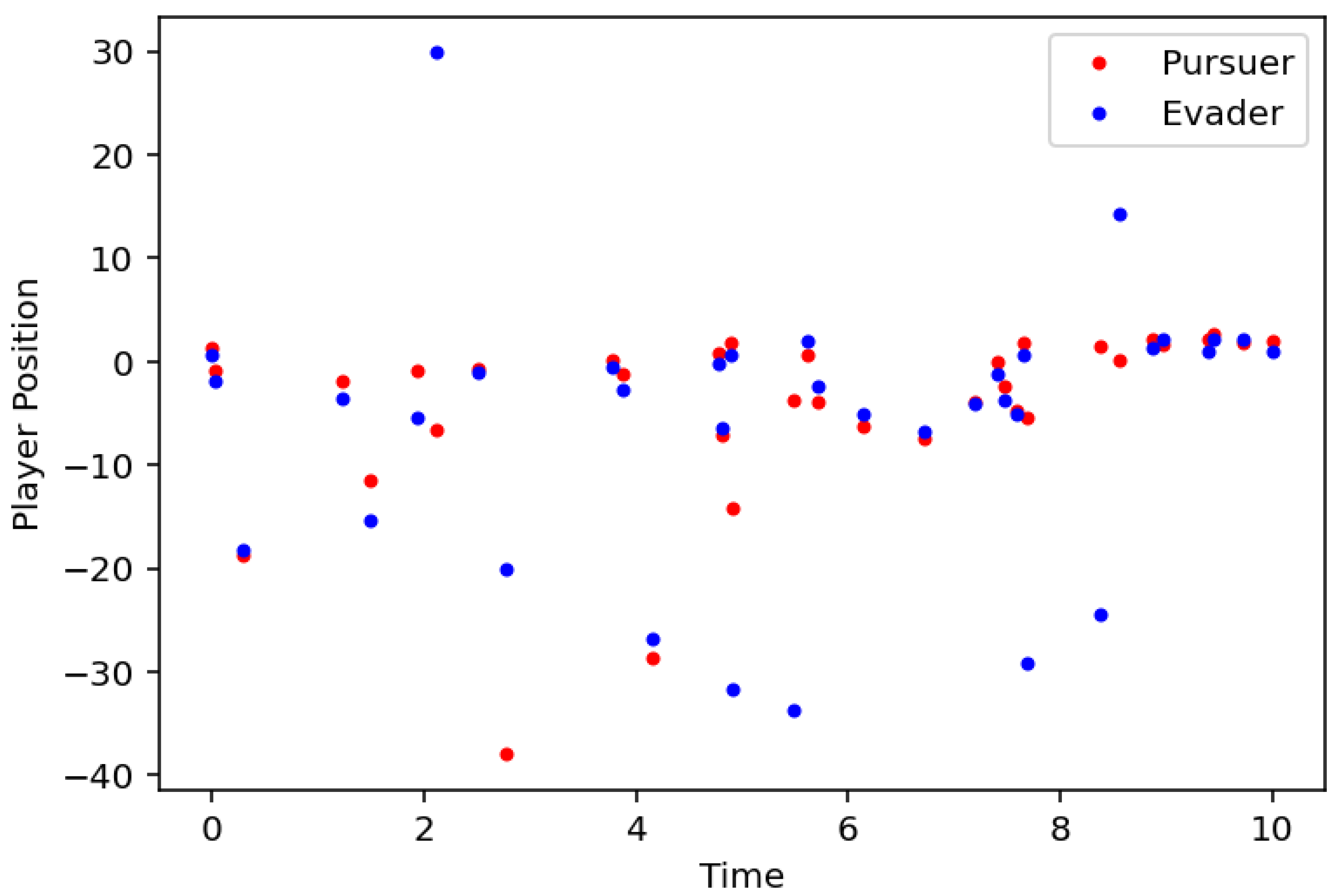
Example 38.

In this last example, we provide a numerical of the LQPEG. In this setting, we sample a two-dimensional pursuer and evader on the same discrete, but uneven time scale

$$\begin{array}{cc}\hfill \mathbb{T}=& \{0,0.03,0.29,1.23,1.49,1.94,2.11,2.51,2.77,3.78,3.87,4.15,4.78,4.81,4.89,\hfill \\ & 4.91,5.49,5.62,5.71,6.15,6.72,7.2,7.4,7.48,7.59,7.66,7.68,8.37,8.55,8.87,\hfill \\ & 8.96,9.4,9.44,9.73,10\}.\hfill \end{array}$$

Next, we consider the theoretical linear dynamic system

$$\begin{array}{ccc}\hfill x_P^{\Delta }\left(t\right)& =& \left[\begin{array}{cc}2& 0\\ 0& 1\end{array}\right]x_P\left(t\right)+\left[\begin{array}{c}1\\ 3\end{array}\right]u\left(t\right),x_P\left(0\right)=\left[\begin{array}{c}2\\ 1\end{array}\right]\hfill \\ \\ \hfill x_E^{\Delta }\left(t\right)& =& \left[\begin{array}{cc}3& 1\\ 1& 1\end{array}\right]x_E\left(t\right)+\left[\begin{array}{c}2\\ -2\end{array}\right]v\left(t\right),x_E\left(0\right)=\left[\begin{array}{c}1\\ 2\end{array}\right].\hfill \end{array}$$

Note that the first component of each player represents its position while the second corresponds to its velocity. For simplicity, only the position is observed. Here, we set the weights in (3.2) to be $R_P=1$, $R_E=1.3$ and $Q=S\left(t_{\mathrm{f}}\right)=I_4$. The plots for the pursuer and evader’s positions are given in Figure 6.1 below.

7. Concluding Remarks and Future Work

In this project, we have established the LQPEG where the pursuer and evader belong to the same arbitrary time scale $\mathbb{T}.$ One potential application of this work is when the evader represented by a drone and the evader represents a missile guidance where their corresponding signals are unevenly sampled. Here. the cost in part represents the wear and tear on the drone. A saddle point in this setting would represent a “live and let live” arrangement, where the drone is allowed to spy briefly on the missile-guidance system and return home, but is not given opportunity to preserve enough of its battery to outstay its welcome. Similarly, in finance the pursuer and evader can represents competing companies where a saddle point would correspond to an effort to coexist, where a hostile takeover or unnecessarily expended resources can be avoided. We have sidestepped the setting where the pursuer and evader each belong to their own time scale ${\mathbb{T}}_P$ and ${\mathbb{T}}_E$, respectively. However, these time scales can be merged using a sample-and-hold method as found in [40,41].

One potential extension of this work is the introduction of additional pursuers. In this setting, the cost must be adjusted to account for the closest pursuer, which can vary over the time scale. A second potential extension is to consider the setting when one player is subject to a delay. Here, both players can still belong to the same time scale. However, this allows one player to act after the other, perhaps with some knowledge of the opposing player’s strategy. Finally, a third possible approach is to such games in a stochastic setting. Here, we can discretize each player’s stochastic linear time-invariant system to a dynamic system on an isolated time scale, as found in [40,42]. However, the usual separability property is not preserved in this setting.

References

- Isaacs, R. Differential Games I, II, III, IV; The RAND Corp. Memo. RM-1391, RM-1399, RM-1411, RM-1486, 1954-1956.
- Isaacs, R. Differential games. A mathematical theory with applications to warfare and pursuit, control and optimization; John Wiley & Sons Inc.: New York, 1965; pp. xvii+384. [CrossRef]
- Kalman, R.E. Contributions to the theory of optimal control. Bol. Soc. Mat. Mexicana (2) 1960, 5, 102–119.
- Kalman, R.E. When is a linear control system optimal? Trans. ASME Ser. D. J. Basic Engineering 1964, 86, 81–90.
- Kalman, R.E.; Koepcke, R.W. Optimal synthesis of linear sampling control systems using generalized performance indexes. Trans. ASME Ser. D. J. Basic Engineering 1958, 80, 1820–1826. [CrossRef]
- Kalman, R.E. The theory of optimal control and the calculus of variations. In Mathematical optimization techniques; Univ. California Press: Berkeley, Calif., 1963; pp. 309–331.
- Ho, Y.C.; Bryson, Jr., A.E.; Baron, S. Differential games and optimal pursuit-evasion strategies. IEEE Trans. Automatic Control 1965, AC-10, 385–389. [CrossRef]
- Bryson, Jr., A.E.; Ho, Y.C. Applied optimal control; Hemisphere Publishing Corp. Washington, D. C., 1975; pp. xiv+481. Optimization, estimation, and control, Revised printing.
- Hilger, S. Ein Maßkettenkalkül mit Anwendung auf Zentrumsmannigfaltigkeiten; PhD Thesis, Universität Würzburg, 1988.
- Bohner, M.; Peterson, A. Dynamic equations on time scales; Birkhäuser Boston Inc.: Boston, MA, 2001; pp. x+358.
- Bohner, M.; Peterson, A., Eds. Advances in dynamic equations on time scales; Birkhäuser Boston Inc.: Boston, MA, 2003; pp. xii+348.
- Bartosiewicz, Z.; Pawłuszewicz, E. Linear control systems on time scales: unification of continuous and discrete. Proceedings of the 10th IEEE International Conference on Methods and Models in Automation and Robotics MMAR’04 2004, pp. 263–266.
- Bartosiewicz, Z.; Pawłuszewicz, E. Realizations of linear control systems on time scales. Control Cybernet. 2006, 35, 769–786. [CrossRef]
- Davis, J.; Gravagne, I.; Jackson, B.; Marks II, R. Controllability, observability, realizability, and stability of dynamic linear systems. Electron. J. Diff. Eqns 2009, 2009, 1–32.
- Fausett, L.V.; Murty, K.N. Controllability, observability and realizability criteria on time scale dynamical systems. Nonlinear Stud. 2004, 11, 627–638.
- Bohner, M.; Wintz, N. Controllability and observability of time-invariant linear dynamic systems. Mathematica Bohemica 2012, 137, 149–163. [CrossRef]
- Bohner, M. Calculus of variations on time scales. Dynam. Systems Appl. 2004, 13, 339–349. [CrossRef]
- DaCunha, J.J. Lyapunov Stability and Floquet Theory for Nonautonomous Linear Dynamic Systems on Time Scales; PhD Thesis, Baylor University, 2004.
- Hilscher, R.; Zeidan, V. Weak maximum principle and accessory problem for control problems on time scales. Nonlinear Anal. 2009, 70, 3209–3226. [CrossRef]
- Bettiol, P.; Bourdin, L. Pontryagin maximum principle for state constrained optimal sampled-data control problems on time scales. ESAIM: Control, Optimisation and Calculus of Variations 2021, 27. [CrossRef]
- Zhu, Y.; Jia, G. Linear Feedback of Mean-Field Stochastic Linear Quadratic Optimal Control Problems on Time Scales. Mathematical Problems in Engineering 2020, 2020, 8051918. [CrossRef]
- Ren, Q.Y.; Sun, J.P.; et al. Optimality necessary conditions for an optimal control problem on time scales. AIMS Math. 2021, 6, 5639–5646. [CrossRef]
- Zhu, Y.; Jia, G. Stochastic Linear Quadratic Control Problem on Time Scales. Discrete Dynamics in Nature and Society 2021, 2021, 5743014. [CrossRef]
- Poulsen, D.; Defoort, M.; Djemai, M. Mean Square Consensus of Double-Integrator Multi-Agent Systems under Intermittent Control: A Stochastic Time Scale Approach. Journal of the Franklin Institute 2019, 356. [CrossRef]
- Duque, C.; Leiva, H. CONTROLLABILITY OF A SEMILINEAR NEUTRAL DYNAMIC EQUATION ON TIME SCALES WITH IMPULSES AND NONLOCAL CONDITIONS. TWMS Journal of Applied and Engineering Mathematics 2023, 13, 975–989.
- Bohner, M.; Wintz, N. The linear quadratic regulator on time scales. Int. J. Difference Equ 2010, 5, 149–174.
- Bohner, M.; Wintz, N. The linear quadratic tracker on time scales. International Journal of Dynamical Systems and Differential Equations 2011, 3, 423–447. [CrossRef]
- Mu, Z.; Jie, T.; Zhou, Z.; Yu, J.; Cao, L. A survey of the pursuit–evasion problem in swarm intelligence, volume = 24, journal = Frontiers of Information Technology & Electronic Engineering, doi = 10.1631/FITEE.2200590, 2023. pp. 1093–1116. [CrossRef]
- Sun, Z.; Sun, H.; Li, P.; Zou, J. Cooperative strategy for pursuit-evasion problem in the presence of static and dynamic obstacles. Ocean Engineering 2023, 279, 114476. [CrossRef]
- Chen, N.; Li, L.; Mao, W. Equilibrium Strategy of the Pursuit-Evasion Game in Three-Dimensional Space. IEEE/CAA Journal of Automatica Sinica 2024, 11, 446–458. [CrossRef]
- Venigalla, C.; Scheeres, D.J. Delta-V-Based Analysis of Spacecraft Pursuit–Evasion Games. Journal of Guidance, Control, and Dynamics 2021, 44, 1961–1971. [CrossRef]
- Feng, Y.; Dai, L.; Gao, J.; Cheng, G. Uncertain pursuit-evasion game. Soft Comput. 2020, 24, 2425–2429. [CrossRef]
- Bertram, J.; Wei, P., An Efficient Algorithm for Multiple-Pursuer-Multiple-Evader Pursuit/Evasion Game; AIAA Scitech 2021 Forum, 2021; [https://arc.aiaa.org/doi/pdf/10.2514/6.2021-1862]. [CrossRef]
- Ye, D.; Shi, M.; Sun, Z. Satellite proximate pursuit-evasion game with different thrust configurations. Aerospace Science and Technology 2020, 99, 105715. [CrossRef]
- Libich, J.; Stehlík, P. Macroeconomic games on time scales. Dynamic Systems and Applications 2008, 5, 274–278.
- Petrov, N.; Mozhegova, E. On a simple pursuit problem on time scales of two coordinated evaders. Chelyabinsk Journal of Physics and Mathematics 2022, 7, 277–286. [CrossRef]
- Mozhegova, E.; Petrov, N. The differential game “Cossacks–robbers” on time scales. Izvestiya Instituta Matematiki i Informatiki Udmurtskogo Gosudarstvennogo Universiteta 2023, 62, 56–70. [CrossRef]
- Minh, V.D.; Phuong, B.L. LINEAR PURSUIT GAMES ON TIME SCALES WITH DELAY IN INFORMATION AND GEOMETRICAL CONSTRAINTS. TNU Journal of Science and Technology 2019, 200, 11–17.
- Lewis, F.L.; Vrabie, D.L.; Syrmos, V.L. Optimal Control; John Wiley & Sons, Inc., 2012. [CrossRef]
- Poulsen, D.; Davis, J.; Gravagne, I. Optimal Control on Stochastic Time Scales. IFAC-PapersOnLine 2017, 50, 14861–14866. [CrossRef]
- Siegmund, S.; Stehlik, P. Time scale-induced asynchronous discrete dynamical systems. Discrete & Continuous Dynamical Systems - B 2017, 22. [CrossRef]
- Poulsen, D.; Wintz, N. The Kalman filter on stochastic time scales. Nonlinear Analysis: Hybrid Systems 2019, 33, 151–161. [CrossRef]
Figure 6.1.
Two-dimensional LQPEG on an isolated, uneven
Disclaimer/Publisher’s Note: The statements, opinions and data contained in all publications are solely those of the individual author(s) and contributor(s) and not of MDPI and/or the editor(s). MDPI and/or the editor(s) disclaim responsibility for any injury to people or property resulting from any ideas, methods, instructions or products referred to in the content. |
© 2025 by the authors. Licensee MDPI, Basel, Switzerland. This article is an open access article distributed under the terms and conditions of the Creative Commons Attribution (CC BY) license (http://creativecommons.org/licenses/by/4.0/).
Copyright: This open access article is published under a Creative Commons CC BY 4.0 license, which permit the free download, distribution, and reuse, provided that the author and preprint are cited in any reuse.