
Submitted:
05 December 2024
Posted:
06 December 2024
You are already at the latest version
Abstract
In this paper we present the main historical facts concerning the Saint Petersburg paradox, the principal solutions that have been proposed, and the results of a new experimental evidence and of a simulation of the game that shed light on the solution of this paradox, that along 300 hundred years since it was first formulated has attracted the attention of many of the most important mathematicians and economists, and that has strongly influenced the development of new concepts adopted in economic and social sciences. The main conclusion is that the behavior of the individuals is not paradoxical at all, and the paradox is intrinsic to the game.
Keywords:
games of chance
; expected utility
; computer simulation
1. Introduction
The Saint Petersburg paradox is probably the oldest and the most famous paradox in decision theory, that gave a fundamental contribution in the birth of the modern theory itself. The fact that, in the simple game of chance proposed, the sum individuals are willing to pay to enter the game is small contradicts the rule that the game should be evaluated according to its (infinite) expected value.
This contradiction and the attempt to solve it has attracted, along 300 years since its first appearance, the attention of many of the most important mathematicians and economists, and has strongly influenced the development of new concepts adopted in economic and social sciences.
This paper reviews the history of this fascinating paradox and the attempts to solve it, and proposes a new study that tries to shed light on the question. In particular, Section 2 describes the birth of the paradox and its discovery by Nicholas Bernoulli. Section 3 presents the first attempts to solve it, while Section 4 discusses more recent proposed solutions of the problem, together with experimental studies that are discussed in Section 5. The new study is illustrated in Section 6, and the conclusions are derived in Section 7.
2. History of the paradox
The origin of the calculus of probability dates back to the 17th century, when in France many aristocrats spent their time and fortunes with games of hazard. One of them, Chevalier de Méré, around 1654 asked the mathematicians Pierre de Fermat and Blaise Pascal to help him in optimum gambling, and their suggestions were based on the expected value of the winnings (in fact Pascal can be considered as the founder of the idea that behavior decisions are based on the expected value of money).
At the beginning of the 18th century, then, the interest originated by the analyses of some games of chance in a book of the mathematician Pierre Reymond de Montmort led to the solutions of technical problems which were incorporated into the developing discipline of probability theory.
Nicholas Bernoulli was the leading figure in stochastics and the games of chance in the second decade of the 18th century, and he was the nephew of the founder of probability theory, James Bernoulli, the most famous representative of the Bernoulli family. After his uncle’s death in 1705, Nicolas Bernoulli undertook the preparation of the latter’s unfinished manuscript on probability for publication. He had a long correspondence with De Montmort and in a letter of 9th September 1713, Nicolas Bernoulli commented on the first edition of Montmort’s treatise (published in 1708) and suggested a number of combinatorial or expectational problems, which were included in the second edition (published in 1713) of the book. In particular, the fourth problem was:
“Apromises to give a crown toBif with an ordinary die he gets six points on the first throw, two crowns if he gets the six on the second throw, three crowns if he gets this point on the third throw, four crowns if he gets it on the fourth, and so on;B’s expectation is required.”
The fitfth problem, then, was:
“The same is required ifApromisesBto give the crowns in the progressionetc. oretc. oretc. oretc. instead ofetc. as before.”
In his response of 15th November 1713 Montmort expressed his opinion that these problems can be solved using geometric progressions and the methods for summation of series developed by Jacob Bernoulli, and in another letter of 20th February 1714 Nicolas Bernoulli demonstrated the importance of his discovery: for the fourth problem he found the sum of the convergent series, but for the first two cases of the fifth problem the game has an expected value of infinity. Indeed, a solution in modern terms of the fourth problem is that the mathematical expectation is:
while for the fifth problem the mathematical expectations for the first two cases do not exist since the series:
and:
both diverge, while in the last two cases the mathematical expectations exist since the series:
and:
both converge. There was therefore a contradiction between the mathematical expectation (that had been accepted in evaluating games of chance), equal to infinity, and the actual sum people were willing to pay in the real world to participate the game.
Montmort expressed skepticism, but had to admit that he was unable to solve this problem.
3. Attempts of Solution
Fifteen years later, Gabriel Cramer, another famous mathematician, read Montmort’s book in which the problem was presented, and in a letter of 21st May 1728 that he addressed Bernoulli first of all simplified the fifth problem by replacing the six-sided die by a two-sided coin and interchanging the roles of A and B, so that success on the trial consists in A tossing a head after having previously tossed consecutive tails, and then receiving crowns from B, Since the mathematical expectation of this gamble is the series of probability weighted payoffs, where each product of payoff and probability is equal to (because the first toss of the coin ends the game yielding 1 crown with probability , the second toss of the coin ends the game yielding 2 crowns with probability , and so on), A’s expectation in this game is given by:
i.e. this series is divergent, and it has no finite expectation. The paradox is therefore that the expected value of the gamble is infinite, but individuals are willing to pay only a small amount to participate in the game. On the contrary, in the fourth of the five problems that Bernoulli presented to Montmort, the expectation was finite, even if the payoff was also unbounded. This problem was identical to the fifth one in terms of probabilities but involved a payoff stream that increased by only 1 crown per toss of the coin rather than by doubling the stakes on each toss, and its expectation is:
To solve the paradox that arises in the fifth problem, Cramer suggested that people evaluate money not in proportion to its quantity but to the utility they can obtain from it. In particular, very big amounts (that in the game considered can be won if heads appears for the first time after a very large number of tosses) give people no more pleasure than amounts equal to a certain threshold. As a consequence, Cramer assumed (arbitrarily) that any amount above crowns was considered equal in value to crowns, hence he assumed the utility function:
and in this case the mathematical expectation of the game becomes:
and then the sum equivalent to the game is the amount c such that:
This value can be further reduced, in particular Cramer considered also a utility function of the form:
since he assumed that the “moral value” of wealth is the square root of the mathematical quantity (e.g. four times the mathematical quantity only yields twice the pleasure). In this case the mathematical expectation becomes:
and then the sum equivalent to the game is the amount c such that:
that is clearly a small amount, close to the one that people attribute as the value of the game considered.
Nicolas Bernoulli, however, did not accept Cramer’s view, who explained why A ought not to give B the equivalent of an infinite sum to play the game, but it did not explain the difference between the mathematical expectation and the ordinary estimate. Bernoulli rejected the argument that the utility deriving from an infinite sum is not greater than that from a finite but very large sum, and concluded that in a game of heads and tails nobody would pay 20 crowns because he would regard his chances of winning a large sum as impossible. He evaluated the expectation as:
saying that the occurrence of the events associated with the sum of the probabilities:
can be disregarded.
In another letter of 27th October 1728 Nicolas Bernoulli communicated the problem in Cramer’s simplified version to his cousin Daniel Bernoulli, another mathematician at the University of Saint Petersburg. In 1728 Daniel answered saying that the paradox has to be found in the small probability that the gamble will last for more than 20 or 30 throws, and individuals are not willing to pay an infinite sum for a gamble in which there is only an infinitesimally small probability of winning, then in 1731 he composed a draft of his famous expected utility theory. The paper was not published until 1738 in the Commentarii of the Saint Petersburg Academy, and from this the paradox became known as “Saint Petersburg paradox”. The formulation of the problem presented by Daniel Bernoulli in his 1738 paper (Bernoulli 1738) is the following:
“Peter tosses a coin and continues to do so until it should land “heads” when it comes to the ground. He agrees to give Paul1ducat if he gets “heads” on the very first throw,2ducats if he gets it on the second,4if on the third,8if on the fourth, and so on, so that with each additional throw the number of ducats he must pay is doubled. What is the maximum amount Paul should pay for this game?”
The solution proposed was to take into account the diminishing marginal utility of money, distinguishing the mathematical expectation from what was called the moral expectation (utility expectation, in modern terms) of a chance event upon which a sum of money depended. The mathematical expectation is defined as the sum of the products of the various sums of money that can be gained times their respective probabilities, i.e.:
while the moral expectation is defined as the sum of the products of the advantages (utilities) accruing from the various sums of money that can be gained times their respective probabilities, i.e.:
Daniel Bernoulli also assumed that the increase in utility as a consequence of an increase in wealth is inversely proportional to the present wealth, i.e:
where is the increment of utility resulting from an increment of wealth, x is the present wealth and is a proportionality factor. Integrating this equation we obtain:
i.e.:
where denotes the initial fortune. In this way, Bernoulli obtained that for a person with initial wealth a that can win the amount (that is ) with probability (that is ), where and , his moral expectation is finite, and is given by:
and the sum of money whose utility equals the moral expectation is the amount c such that:
from which:
From this formula it follows that if Paul doesn’t have an initial wealth (i.e. ) the worth of the gamble to him is given by:
while if then , if then and if then . As outlined by Bernoulli, therefore, Paul’s prospective gain will increase with the size of Paul’s fortune but will never attain an infinite value unless Paul’s wealth simultaneously becomes infinite. In particular, the worth of the gamble to Paul, possessing small resources, is quite small, and increases only slowly with the magnitude of his fortune. In this way Daniel Bernoulli tried to solve the paradox.
Nicholas Bernoulli was not completely satisfied with this explanation, in any case he thought that matching together the idea of Daniel Bernoulli, that of Gabriel Cramer and his own, according to which it is necessary to estimate a small probability as null, it is possible to find a finite expected value of the Petersburg gamble, and also to determine exactly the equivalent value of this gamble.
4. More Recent Attempts
During the following 200 years, Daniel Bernoulli’s utility theory was discussed and generalized. Finally, in 1934 Karl Menger showed that utility must be bounded from above (Menger 1934). In fact, given Bernoulli’s logarithmic utility function, the paradox appears again if the payoffs grow sufficiently fast. For instance, in a St. Petersburg game with logarithmic utility in which Paul receives ducats if the first head is obtained at the th toss, Paul’s expected utility is:
i.e. it is infinite, and the paradox returns. If a new, unbounded utility function were introduced for this game so as to return a finite expectation, then a new set of more rapidly increasing payoffs can be designed so that the resulting expectation again is infinite. Samuelson called this result “Menger’s Super-Petersburg Paradox” (Samuelson 1977). By repeatedly adjusting the payoff strategy, the measurement of utility by logarithms can always be made to result in an infinite expectation, and it becomes clear that the paradox can be avoided if and only if the utility function is bounded.
Menger’s paper also played a crucial role in persuading von Neumann and Morgenstern to develop a formal treatment of utility, and the axiomatic approach to expected utility was incorporated in the second edition of their fundamental book “Theory of Games and Economic Behavior” (Von Neumann and Morgenstern 1947). In 1971, then, Arrow showed that to avoid the Super-Petersburg paradox the utility function must be bounded from both above and below (Arrow 1971).
During the last 3 centuries since Nicolas Bernoulli proposed his fourth and fifth problems to De Montmort in 1713, numerous solutions of the Saint Petersburg paradox have been proposed. Some authors such as D’Alembert attacked the bases of probability, others such as Lubbock, Drinkwater and De Morgan accepted the view that A was justified in paying an infinite sum to B because his expectation was infinite. Fontaine, a French mathematician, assumed that the banker’s capital is finite and sought the stake that the player should pay to make the game equitable, obtaining in this way some inequalities for the number of games to be played under these constraints.
Other contributions to the discussion of the paradox are those of Buffon (1777). First of all he developed Fontaine’s idea further, taking into account the banker’s ability to fulfill his obligation, in particular paying off the player after a long sequence of tails has arisen before the first head appears. He pointed out that if a head does not appear until after the 29-th toss, there would be no sufficient money in the whole French kingdom to pay the player (he also made an estimate of the number of games which would be possible in a player’s lifetime).
The view that the limitation of the banker’s capital implies that only the restricted game is possible in the real world was adopted by many later writers on the Saint Petersburg paradox such as Poisson, Catalan, Czuber, Pringsheim, Von Mises, and it is perhaps the most frequently offered resolution of the paradox. In this case the boundedness of the winnings is justified by the finiteness of the bookmaker’s wealth or by the fact that the time of playing a Saint Petersburg game cannot be infinitely long. However it also had opponents, for example Bertrand suggested that, whatever the banker owes, he can compensate the player, wheter he is solvent or not, by simply writing a note for the debt. Further elaborations were given by Shapley and Samuelson (Shapley 1977, Samuelson 1977).
Buffon suggested another possibility relevant to the solution of the paradox, i.e. the fact that any probability below some small positive fraction can be set equal to zero: in particular he considered a probability of or less for an event as a probability which may be disregarded (since this was the probability that a 56-year old man in good health would die within 24 hours). Daniel Bernoulli approved this idea, but more conservatively chose a threshold, called “moral probability” , of . Also Fontaine, Poisson, Condorcet and D’Alembert accepted the idea of negligible probabilities, and perhaps the most important proponent of negligible probabilities in moder times was the French mathematician Borel who considered as negligible, with reference to the Saint Petersburg paradox, possible results with probability lower than .
Buffon also tested his arguments, and to this end he conducted the first recorded experiment in statistics to determine empirically the likely outcomes in the Petersburg gamble. A child played out trials of the Petersburg gamble, all these trials ended after at most nine tosses and the average payoff was ducats, hence he concluded that about 5 ducats should be a fair entry fee to the gamble (compared with the units per game predicted by the theoretical argument).
In the 1930’s and 1940’s, then, considerable attention was given by probabilists to increasingly general formulations of the law of large numbers, and in particular Feller gave a result that is directly applicable to the Saint Petersburg problem. More precisely, he considered the total gain in N games and proved that a modified law of large numbers holds for it (Feller 1945). To compare these estimates with the experimental results previously obtained, some computer simulations were made involving 22528 Saint Petersburg games, and the resulting average payout turned out to be units per game, compared with the Feller’s estimate of units per game and with Buffon’s estimate of units per game. In 1985, then, Martin-Lof obtained a limit theorem for the total gain in a series of Saint Petersburg games, that can be regarded as a sharpening of Feller’s result (Martin-Lof 1985).
An alternative resolution to the Petersburg paradox is the so-called “expectancy heuristic”, proposed by Treisman. Instead of computing the product of probabilities and payoffs, the expectancy heuristic suggests computing the outcome at the expected gamble length. In the Petersburg gamble, the number of trials to obtain the first head is i with probability , therefore the expected number of trials that it would take for the first head to occur is:
and rearranging the terms:
and then regrouping them:
where each regrouping is a geometric series whose sums are:
therefore the initial expression corresponds to:
and this means that the gamble is expected to terminate on the second trial, therefore the expected length is 2. As a consequence, the corresponding payoff is 2 ducats, which is therefore the value of the Petersburg gamble according to the expectancy heuristic (Treisman 1983).
Summarizing, there have been three types of solutions offered to the paradox. The first, attributed to Poisson and Condorcet, is that the conditions of the game itself imply a contradiction, since the game, by promising to pay an infinite sum, implies a condition which can not be fulfilled. In addition, lack of time is another limitation for the gamble to be well-defined, since it could be that, once started, the gamble never ends, but in the real world nobody can toss a coin an infinite number of times.
The second type of solution, attributed to Buffon, is the principle that events whose probabilities are sufficiently small, can be regarded as impossible. As a consequence, since the probability that a head will not appear until the toss becomes very small for i sufficiently large, if the occurrence of that event is regarded as impossible for all n beyond a certain value, the mathematical expectation of returns becomes finite, and the paradox is resolved.
The third type of solution, attributed to Daniel Bernoulli, is to assume that the marginal utility of money is decreasing, so that the expected value of the game is finite. An objection to this solution was pointed out by Menger, that showed that the paradox can be restored by modifying the game such that the payoff grows sufficiently fast: in this situation, this difficulty can be avoided by requiring that the utility function be finite.
As outlined by Yukalov “...The St. Petersburg paradox is probably the oldest paradox in decision theory and has promoted the birth of modern decision theory itself.[...] In economics, it has played a particularly important role in pointing out situations in which supposedly rational decisions based on expected gains or even expected increasing utilities are not endorsed by real rational human decision makers. This paradox has opened a flood of attempts to solve it, which turn out all to modify it in one way or another. The most important change involves the introduction of a concave utility function, which captures the idea (due to Cramer) that individuals estimate money in proportion to the usage that they may make of it, and not necessarily in proportion to its quantity. Motivated by the St. Petersburg paradox, the introduction of concave utility functions, which embody risk aversion and decreasing marginal utility of gains, remains the central pillar of modern economic theory. However, the solution in terms of utility functions of Cramer and Bernoulli is not completely satisfactory since a slight change in the formulation makes the paradox reappear.
The conclusion is that from the mathematical and logical point of view, the St. Petersburg paradox is impeccable, while the suggested solutions are not mathematical, since they all modify the initial problem, hence the original St. Petersburg paradox remains unresolved." (Yukalov 2021).
5. Experimental Studies
Despite the age and the importance of the problem only a few experiments on the Petersburg gamble have been documented, probably due to the fact that the solvency problem renders the experimental approach to the gamble meaningless. To avoid this problem the experimental design must involve the truncated gamble, that is therefore limited to a finite number of possible tosses. This setting has been used in a study by Cox et al. (2007), in a study by Hayden and Platt (2009) and in a study by Neugebauer (2010). From these studies it seems that a majority of subjects in the experiments are risk averse, not risk neutral, and that in the case of repeated gamble subjects’ valuations converge to the median outcome, hence giving acknowledgement to the proposal of Tolman and Foster (1981) that the median valuation is a reasonable choice for the repeated Petersburg gamble.
In the experimental study of Neugebauer (2010) the one-shot Petersburg gamble is considered. The underlying assumption is that preferences are represented by the general expected utility functional form:
Most of the various hypoteses that have been put forth in the history of the paradox truncate the Petersburg gamble, including the bounded utility or the finite wealth hypotheses, which put an upper bound on the utility of the gamble, and the physical impossibility or the moral impossibility hypotheses, which assume that a small probability is set equal to zero, i.e. for p. The objective of the experimental study is to understand if it is possible to find evidence for such a cut-off level and, if so, at what level this cut-off would occur. First of all, the study shows that it seems that people neglect small probability events in the Petersburg gamble. In effect, from the experiment there is some evidence that subjects’ valuations for the longer gamble are not higher than for the shorter game, from which it seems that the probabilities are set equal to zero at or below a certain probability level. It is therefore important to determine the probability level at which the probabilities are truncated in the Petersburg gamble. In particular, from the experiment it seems that probabilities smaller than are neglected by experimental subjects, and this result is in line with the conjecture of Nicholas Bernoulli that a probability smaller than should be set equal to zero in the Petersburg gamble. His computation was in fact:
therefore it did not account for any payoffs above 16 ducats. If the gamble is limited to five tosses, the maximum payoff of 16 ducats occurs with probability , implying an expected payoff of ducats. After computing the expected value, Nicholas Bernoulli also admitted that decreasing marginal utility may play a role in the valuation. The results of the experiment of Neugebauer also show that the willingness-to-pay exhibits an age effect (the more senior individuals who participated in the experiment have a higher willingness-to-pay), furthermore subjects’ offers increase significantly with income (in line with the assumption of Daniel Bernoulli, according to which the willingness-to-pay for the Petersburg gamble should be an increasing function of wealth). In addition, the small probability neglect effect is robust to subject-pool changes, and the results show that longer gambles get no higher valuation than the five-toss gamble, hence subjects’ valuations are as if they truncate probabilities smaller than in the Petersburg gamble.
In conclusion, the Petersburg problem originally was designed to study the level of moral impossibility in games of chance. During the life-time of Nicholas Bernoulli there was little interest in studying moral impossibilities in the games of chance and, generally, in applications to the social sciences, but as a consequence of the fact that Daniel Bernoulli published the expected utility concept as a solution to the Petersburg paradox, the problem received contributions through the centuries by some of the most brilliant minds. In particular, Nicholas Bernoulli derived a level of moral impossibility of to determine the fair value of the Petersburg gamble, and beyond that level each smaller probability is unlikely. The experiments conducted support this conclusion, and therefore it seems reasonable to accept that the neglect of small probability events is a more relevant solution criterion in the Petersburg paradox than its best known alternatives, bounded utility and the limitation of the experimenter’s expected wealth.
6. A New Study: Materials, Methods, Results and Discussion
In order to shed ligth on the nature of the Saint Petersburg paradox, we have undertaken a new study, proceeding in two directions. On the one hand, an extensive experiment has been conducted, involving a large number of individuals, to which the participation in the Saint Petersburg game has been proposed, in order to understand their behavior. On the other hand, a computer simulation of the game has been performed, in order to compare the results to the actual behavior of the individuals.
6.1. The experiment
With reference to the first part of the study, i.e. the experiment, it has involved a large number of students of the School of Economics of the University of Turin, enrolled in different years of study, distinguishing between undergraduate and Master level, and between Business-oriented students and Economics-oriented students.
Table 1 reports the groups of students involved in the experiment and their numbers:
These data are also represented in Figure 1:
All these students have been faced with 3 questions, in which they were asked to evaluate, respectively, the version of the game that doesn’t give rise to the paradox, then the “truncated version” and finally the original version of Saint Petersburg game.
The first question, formulated in order to evaluate the version of the game that doesn’t generate the paradox (and corresponding to the fourth problem that Nicholas Bernoulli originally proposed to Montmort) was the following:
“You can enter a game in which a coin is flipped until heads occurs for the first time. You win1€ if heads appears for the first time at the first toss, you win2€if heads appears for the first time at the second toss, you win3€if heads appears for the first time at the third toss, you win4€if heads appears for the first time at the fourth toss, and so on. How much are you willing to pay to participate in this game?”
The second question, formulated in order to evaluate the “truncated version” of the game, was the following:
“You can enter a game in which a coin is flipped until heads occurs for the first time. You win1€if heads appears for the first time at the first toss, you win2€if heads appears for the first time at the second toss, you win4€if heads appears for the first time at the third toss, you win8€if heads appears for the first time at the fourth toss, and so on. However, if after7tosses heads has not appeared, the game ends and you don’t ’win anything. How much are you willing to pay to participate in this game?”
The third question, formulated in order to evaluate the original version of the game, was instead the following:
“You can enter the same game of the previous question, but this time the game ends only when heads appears for the first time (eventually after a large number of tosses). Also in this case, each additional toss is associated with a payoff that is the double of the previous one. How much are you willing to pay to participate in this game?”
The reason of these questions was the intention to investigate if, with reference to the version of the problem that doesn’t give an infinite expected payoff, the behavior of the individuals is consistent with the theory, and if, with reference to the version that generates the infinite expected payoff, moving from a reduced (in the truncated version) to a potentially very large (in the complete version) number of tosses, the evaluation of the game by the individuals was very different.
Table 2 reports the results of the experiment, indicating for each group of students the average amount that the individuals of the group considered are willing to pay to participate in each of the three versions of the game.
These results are also represented in Figure 2:
From these results, the main conclusions that emerge are the following:
- Business-oriented students are willing to pay a higher amount than Economics-oriented students to participate in the game.
- Younger students are willing to pay a higher amount than older students, both in the Business-oriented group and in the Economics-oriented one.
- For the first version of the game, Business-oriented students are willing to pay an amount that is slightly higher than the expected value of the game (in this case, as shown above, the expected payoff is equal to 2€), while Economics-oriented students are willing to pay an amount that is lower than this expected value.
-
All groups of students, both at the undergraduate and at the Master level, are willing to pay for the truncated version of the game a sum that is lower than the expected value for the game, that in this case is:This sum ranges from € to €, revealing that individuals expect that heads will appear for the first time after around 3 tosses. At the same time, all the groups of students are willing to pay, to enter the complete version of the game, a sum that is higher than that for the truncated version, but that is lower than the amount gained if head appears for the first time after 4 tosses, and that is clearly enormously lower than the potentially very large amount that the complete version of the game could allow to win.
In general, the sums declared as amounts that individuals are willing to pay to enter the game (both in the truncated and in the complete version) reveal that they expect the game will end after 3 or 4 tosses of the coin.
6.2. The Simulation of the Game
With reference to the second part of the study, a computer simulation of the game has been developed. Using Python language (see the Appendix for the code), a program has been written in order to simulate the throws of the coin. If heads appears for the first time at the i-th toss, the game ends and a payoff of is registered, otherwise a new toss of the coin is performed and the game continues, until heads appears. Moreover, at the end of all the simulations the average number of coin tosses and the average payoff obtained are computed. Different blocks of simulations have been performed (first of all a block of simulations, then another block of simulations, and so on), and the results are reported in Table 3 :
In this table the first column indicates the number of simulations performed, taking into account that a single simulation starts with the toss of a coin and ends when heads appears for the first time. At the end of each block of simulations (for example in the first row after simulations, in the second row after simulations, and so on) the program computes the average payoff obtained, that is:
and the corresponding results are reported in the second column. Always at the end of each series of simulations the program computes the average number of coin tosses, that is:
and the corresponding results are reported in the third column. Finally, the fourth column reports, for each block of simulations, the maximum number of coin tosses that, in that block, has been necessary to obtain heads for the first time, and therefore to end the game (this is a measure of the “extreme events” in the game).
The results are represented also in Figure 3:
From these results the main conclusions are the following:
- First of all, as n increases (starting from to simulations) the average number of coin tosses converges to 2, that in effect is the expected value of the number of tosses for this problem. For example, when simulations are performed the game ends on average after tosses, when n increases to and then to simulations the game ends on average after tosses, and when the number of simulations is increased further to and over the average number of coin tosses that are necessary to end the game is 2.
- The average payoff obtained from the game shows a more erratic behavior. When simulations are performed the average payoff of the game is €, while when the number of simulations increases to and then to the average payoff turns out to be € and € respectively, and when n increases further to and then to the average payoff rises to € and then to €.
- The maximum number of coin tosses performed in each simulation before obtaining heads for the first time, instead, has a clear monotonic behavior with respect to the numer of simulations. When or simulations are performed the maximum length of the game is 15 tosses, when and then simulations are considered this length increases to 17 and 18 tosses, and when and simulations are performed the length reaches 20 tosses.
In general, the conclusion that emerges from these simulations of the game is that the number of coin tosses after which the first head appears is quite small (in fact the expcted number of tosses to end the game, as shown above, is 2, i.e. we expect that the game ends after 2 tosses of the coin), and as a consequence also the payoff obtained is small. In our study, for instance, the number of simulations ranges from to , and the corresponding average number of coin flips ranges from to 2, while the average payoff goes from € to €. There are, of course, the “extreme events”, reported in the last column of the table, when head appears for the first time only after 20 tosses or around it, but they are precisely “extreme” and rare. In this sense, the behavior of the individuals, that (as shown by the previous experiment) are willing to pay only a small amount to enter the game, is consistent with the results of the simulations.
7. Conclusions
The experiment reported shows that the individuals involved in the game expect that heads will appear for the first time (and the game will end) after 3 or 4 tosses, and for this reason they are not disposed to pay more than 3 to 5€ to participate in the game. The simulations show that the average number of tosses is around 2 (that is in fact the expected value of the number of coin flips in this game) and therefore the behavior of the individuals is consistent with this result, and not paradoxical at all.
Put in other terms, the individuals (correctly) neglect the very small probabilities associated with very large payoffs, that are responsible of the infinite expected value of the game (in the complete version), and consider such probabilities as equal to 0. The paradox of the Saint Petersburg game, therefore, stems not from the behavior of the individuals, but from the mathematical structure of the problem, i.e. from the fact that for a particular payoff structures (i.e. when the payoffs double at each subsequent round of the game) the expected value turns out to be infinite. It is the divergence of the series:
that makes the expected value of the game infinite, and that creates the paradox, not the behavior of the individuals. In this sense the paradox is intrinsic to the game (and the solutions proposed to solve it are not completely satisfactory, since in any case they determine a change in the original structure of the problem), and the only thing we can recognize, as Martin (2008) concludes, is that “The St. Petersburg result is strange... The appropriate reaction might just be to try to accept the strange result”.
Funding
This research received no external funding.
Informed Consent Statement
Informed consent was obtained from all subjects involved in the study.
Data Availability Statement
The data collected for this research are available upon request from the author. The Pyhton code used for simulations is available in the Appendix.
Acknowledgments
We thank Federico Nervi and Alberto Turigliatto for their help in the simulation of the game considered in the study.
Conflicts of Interest
The author declares no conflicts of interest.
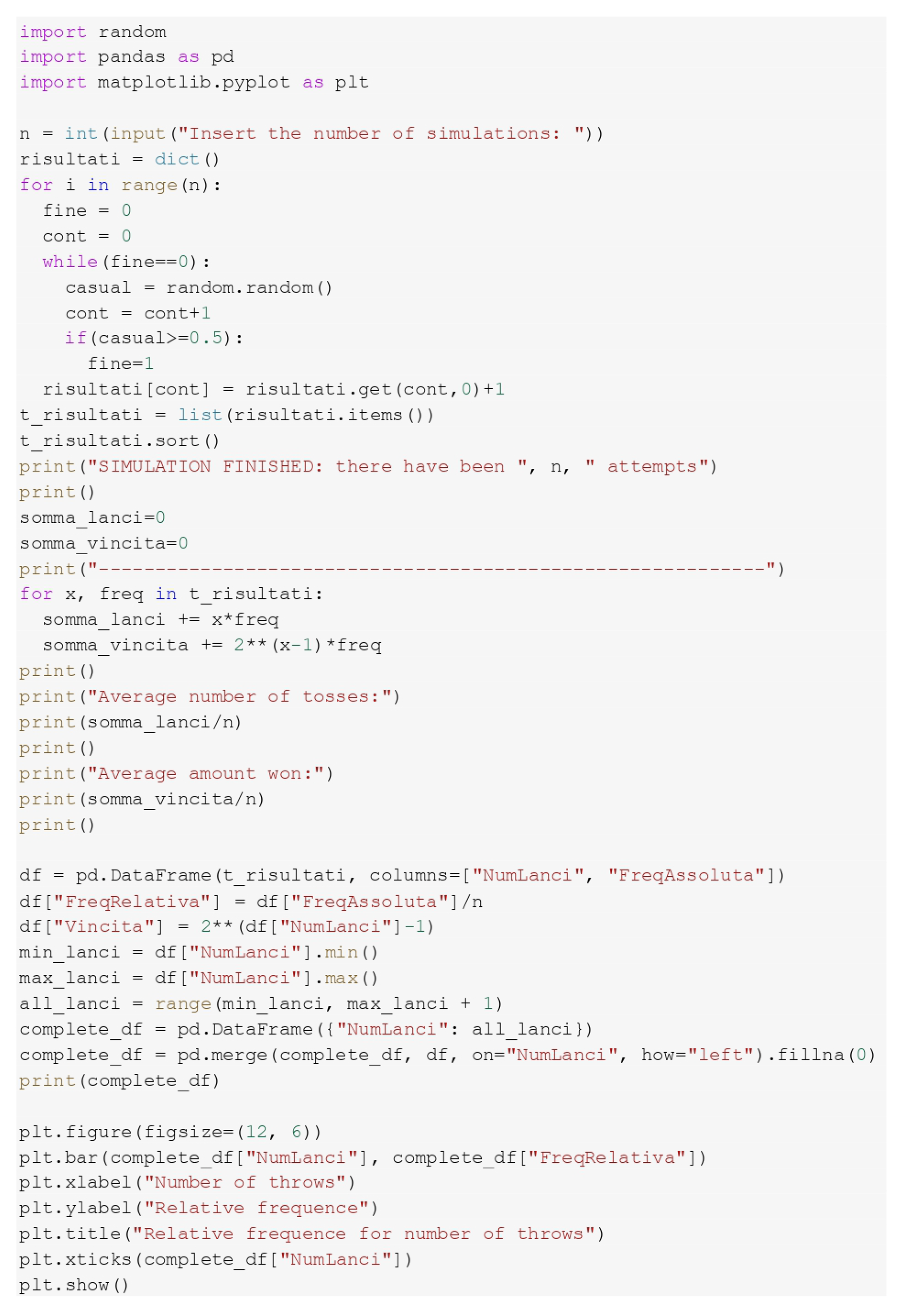
Appendix A
This Appendix reports the Python code used to simulate the game considered in the study.
Figure A1.
Python code used for the simulations of the game.
References
- Arrow, K. J. Essays in the theory of risk-bearing., Amsterdam and London, 1971; pp. 44–89.
- Aumann, R. J. The St. Petersburg paradox: A discussion of some recent comments. Journal of Economic Theory 1977, 14, 443–445. [Google Scholar] [CrossRef]
- Bassett, G. W. The St. Petersburg paradox and bounded utility. History of Political Economy 1987, 19(4), 517–523. [Google Scholar] [CrossRef]
- Bernoulli, D. Exposition of a new theory on the measurement of risk. Proceedings of the Imperial Academy of Sciences of St. Petersburg 1954, 5, 175–192. [Google Scholar] [CrossRef]
- Buffon, G. L. Essai d‘arithmétique morale. In Supplément à l‘historie naturelle 1777, IV; reproduced in Un autre Buffon; Hermann; 1977; pp. 47–59.
- Ceasar, A. J. The Saint Petersburg paradox and some related series. The Two-Year College Mathematics Journal.
- Ceasar, A. J. A Monte Carlo Simulation Related to the St. Petersburg Paradox. College Mathematical Journal 1984, 15(4), 339–342. [Google Scholar] [CrossRef]
- Cox, J. C.; Sadiraj, V.; Vogt, B.; Dasgupta, U. Is there a plausible theory for risky decisions? Georgia State University, Experimental Economics Center Working Paper 2007 – 05, 2007.
- Dutka, J. On the St. Petersburg paradox. Archive History of Exact Sciences 1988, 39, 13–39. [Google Scholar] [CrossRef]
- Feller, W. Note on the Law of Large Numbers and Fair Games. Annals of Mathematical Statistics 1945, 16, 301–304. [Google Scholar] [CrossRef]
- Hayden, B.Y.; Platt, M.L. The Mean, the Median, and the St. Petersburg Paradox. Judgment and Decision Making 2009, 4(4), 256–272. [Google Scholar] [CrossRef]
- Klyve, D.; Lauren, A. An empirical approach to the St. Petersburg paradox. The College Mathematics Journal 2011, 42(4), 260–264. [Google Scholar] [CrossRef]
- Martin, R.M. The St. Petersburg paradox. In Stanford Encyclopedia of Philosophy; 2008; Stanford University, Stanford.
- Martin-Löf, A. A Limit Theorem Which Clarifies the Petersburg Paradox. Journal of Applied Probability 1985, 22, 634–643. [Google Scholar] [CrossRef]
- Menger, K. Das Unsicherheitsmoment in der Wertlehre. Zeitschrift der Nationalökonomie 1934, 51, 459–485. [Google Scholar] [CrossRef]
- Neugebauer, T. Moral impossibility in the St Petersburg paradox: A literature survey and experimental evidence, Luxembourg School of Finance Working Paper, 1–43, 2010.
- Samuelson, P.A. The St. Petersburg Paradox as a Divergent Double Limit. International Economic Review 1960, 1, 30–37. [Google Scholar] [CrossRef]
- Samuelson, P.A. St. Petersburg paradoxes: defanged, dissected, and historically described. Journal of Economic Literature 1977, 15, 25–55. [Google Scholar]
- Seidl, C. The St. Petersburg paradox at 300. Journal of Risk and Uncertainty 2013, 46, 247–264. [Google Scholar] [CrossRef]
- Shapley, L. S. The Petersburg Paradox. A con game? Journal of Economic Theory 1977, 14, 439–442. [Google Scholar] [CrossRef]
- Tolman, D. C.; Foster, J. H. Buffon, the computer and the Petersburg paradox. In Probability and Statistics; pp. 161–169.
- Treisman, M. A solution to the Petersburg paradox. British Journal of Mathematical and Statistical Psychology 1983, 9, 224–227. [Google Scholar] [CrossRef]
- Von Neumann, J.; Morgenstern, O. Theory of games and economic behavior, 2nd ed.; Princeton University Press, Princeton; 1947.
- Yukalov, V.I. A Resolution of St. Petersburg Paradox. Journal of Mathematical Economics 2021, 97, 1–12. [Google Scholar] [CrossRef]
Figure 1.
Number of students involved in the experiment.
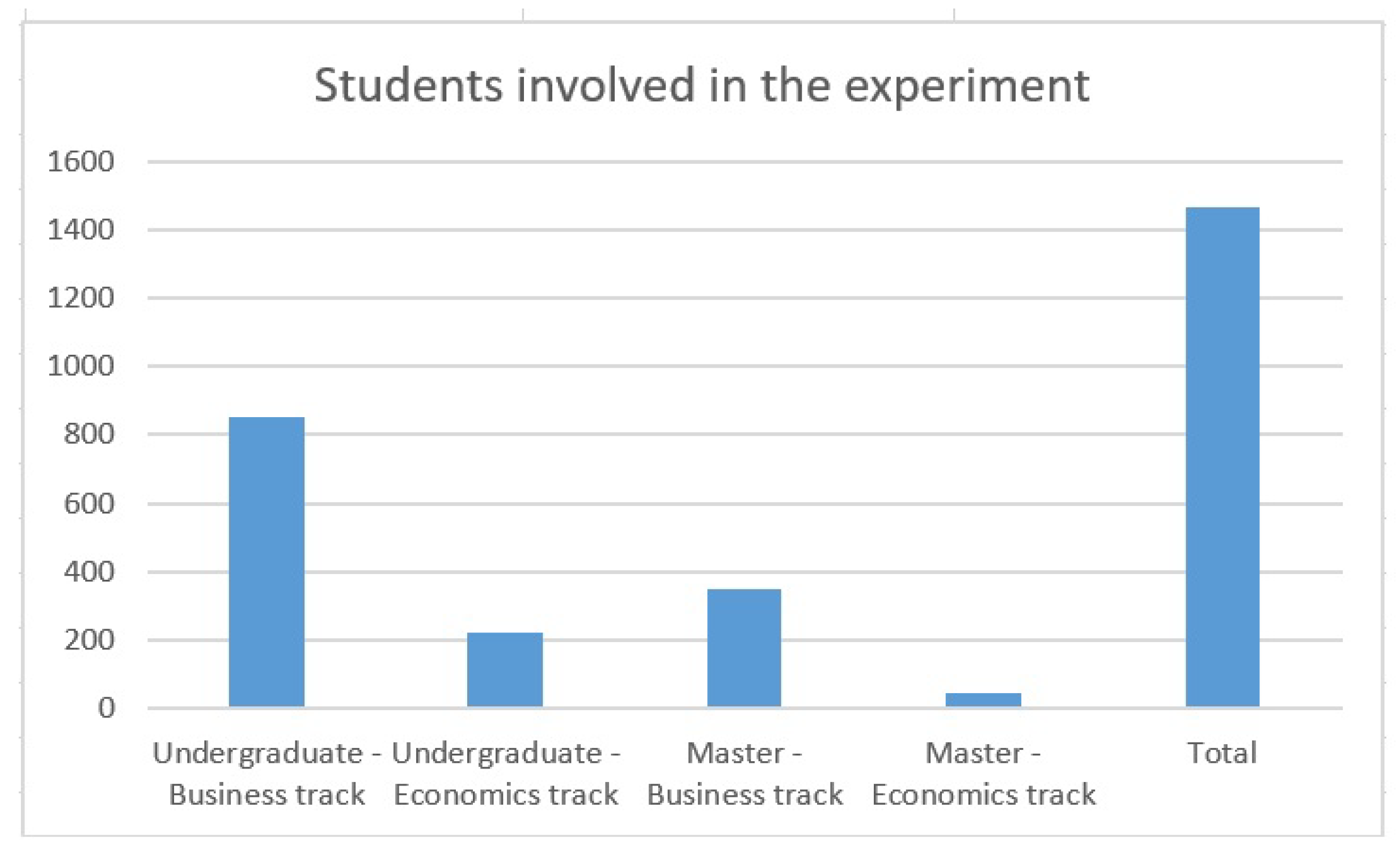
Figure 2.
Average amounts paid to enter the game.
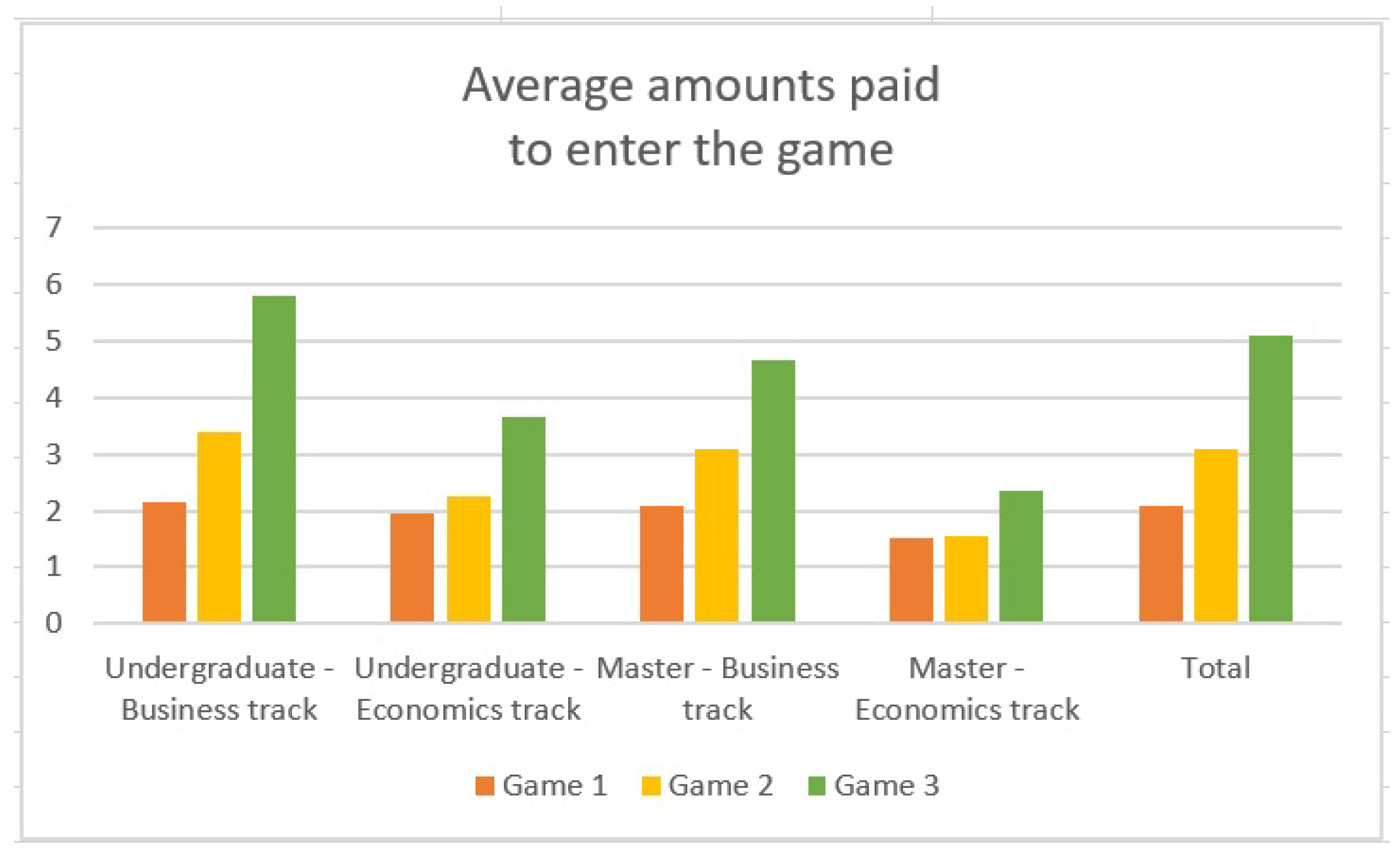
Figure 3.
Results of the simulations.
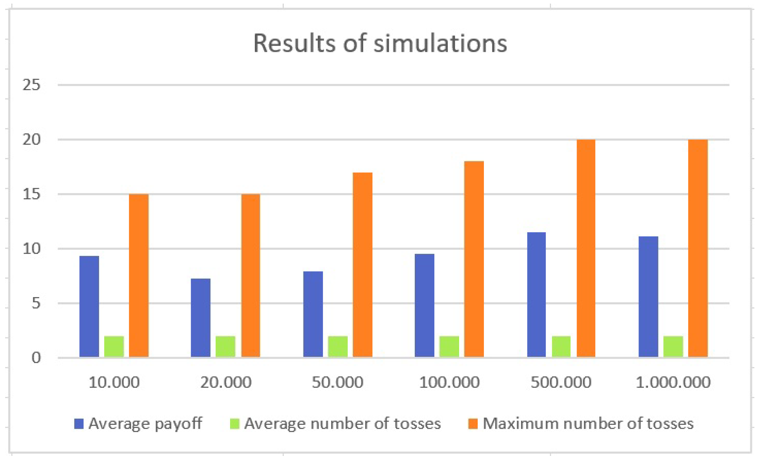

Table 1.
Groups of students involved in the experiment.
| Groups of students | Number of students |
|---|---|
| Undergraduate students - Business track | 850 |
| Undergraduate students - Economics track | 220 |
| Master students - Business track | 350 |
| Master students - Economics track | 45 |
| Total | 1465 |
Table 2.
Results of the experiment.
| Group of students | Average amount game 1 | Average amount game 2 | Average amount game 3 |
|---|---|---|---|
| Undergraduate students - Business track | 2.15 € | 3.38 € | 5.78 € |
| Undergraduate students - Economics track | 1.95 € | 2.26 € | 3.65 € |
| Master students - Business track | 2.10 € | 3.07 € | 4.65 € |
| Master students - Economics track | 1.50 € | 1.54 € | 2.34 € |
| Total | 2.09 € | 3.08 € | 5.08 € |
Table 3.
Results of the simulations.
| Number of simulations | Average payoff | Average number of tosses | Maximum number of tosses |
|---|---|---|---|
| 10,000 | 9.31 € | 1.97 | 15 |
| 20,000 | 7.28 € | 1.98 | 15 |
| 50,000 | 7.95 € | 1.98 | 17 |
| 100,000 | 9.51 € | 2 | 18 |
| 500,000 | 11.54 € | 2 | 20 |
| 1,000,000 | 11.14 € | 2 | 20 |
Disclaimer/Publisher’s Note: The statements, opinions and data contained in all publications are solely those of the individual author(s) and contributor(s) and not of MDPI and/or the editor(s). MDPI and/or the editor(s) disclaim responsibility for any injury to people or property resulting from any ideas, methods, instructions or products referred to in the content. |
© 2024 by the authors. Licensee MDPI, Basel, Switzerland. This article is an open access article distributed under the terms and conditions of the Creative Commons Attribution (CC BY) license (http://creativecommons.org/licenses/by/4.0/).
Copyright: This open access article is published under a Creative Commons CC BY 4.0 license, which permit the free download, distribution, and reuse, provided that the author and preprint are cited in any reuse.


