
Submitted:
16 April 2025
Posted:
21 April 2025
You are already at the latest version
Abstract
This study presents the algorithm - Victoria - an approach that demonstrates there are parameters φ, k, j considered optimal that guarantee the player will always have an advantage over the house in sports betting field in the medium and long run with guaranteed satisfactory profits. After n Small Blocks (j n ) and Intermediate Blocks (IBs) containing k independent events with the same probability p, we conclude that the cost-benefit ratio over the value in a sequence of independent events β (success block) > ζ (failure block) is always the case. Taking into account the possible impacts of Victoria on Decision Theory as well as Game Theory, a function η(X t ) called “Predictable Random Component” was also observed and presented. The η(X t ) function (or fv(X t ) in the context of VNAE) refers to the fact that within a game in which the randomness factor in a uniform distribution is crucial to it, any player who has advanced knowledge of randomness added to other additional actions, whether with the support of statistics, mathematical, physical operations and/or other cognitive actions, will be able to determine an optimal strategy whose results of the expected value of the player's payoff will always be positive regardless of what happens after n sequences determined by the player. In addition, the possibility of the existence of a new equilibrium was also observed, thus resulting in the Victoria-Nash Asymmetric Equilibrium (VNAE) theorization. We develop a rigorous statistical foundation, incorporating Markov processes, Brouwer’s fixed-point theorem, and statistics convergence to validate the existence of asymmetrical advantages in structured random systems. And anchored by the Stirling Numbers, the Law of Large Numbers, the Central Limit Theorem, Kelly's Criterion, Renewal Theory, Unified Neutral Theory of Biodiversity, Nash Equilibrium and Monte Carlo simulation itself, for example, the proposed new equilibrium is expected to be a solid mathematical model suitable for modeling games in which one of the players tends to have asymmetric advantages. In this sense, VNAE is an extension of the classic Nash Equilibrium, Stackelberg Equilibrium, and Bayesian Equilibrium. Victoria has shown that by understanding the general behavior of randomness through statistics, we can, in a way, partially “predict” the future and shape it in our favor. Furthermore, in Game Theory, it is hoped that the impact could be relevant to better understanding and adapting concepts such as stochastic games, asymmetric games, zero-sum games, repeated games and imperfect information games, for example. By bridging gaps between theory and real-world applications, this work positions the VNAE as a foundational tool for interdisciplinary advancements in decision-making under uncertainty.
Keywords:
Randomness
; Sports Betting
; Decision Theory
; Game Theory
; Statistics
; Probability Theory
1. Introduction
The study of randomness and its application in different areas of knowledge has been a recurring theme in statistics, game theory and behavioral economics. Traditionally, games of chance and sports betting are structured in such a way as to guarantee a statistical advantage for the house, making overcoming this model a mathematical and theoretical challenge. However, this study presents the Victoria methodology, an approach based on statistics and the true nature of randomness that proposes a new paradigm: the possibility of achieving a sustainable advantage for the bettor in the long term.
The research assumes that it is possible to identify optimal configurations/parameters - φ, k and j - that will - at least theoretically - ensure a mathematical expectation for the gambler.
Through a rigorous probabilistic model, anchored in the convergence of probability, the Law of Large Numbers, the Central Limit Theorem and Monte Carlo simulations, the study shows that certain configurations allow the player to obtain a return greater than the risk involved in the long term.
In addition, the author, anchoring himself in the rich bibliography left by his colleagues over time, such as Stirling Numbers, Renewal Theory, Unified Neutral Theory of Biodiversity, Nash Equilibrium, Kelly Criterion, among other related topics, proposes the Predictable Random Component (η) function in game theory. This function η(Xt) (or fv(Xt), in VNAE) suggests that, even in scenarios dominated by randomness, advanced knowledge of probability distributions and randomness can significantly influence the expected results, even in a game whose basis is dominated by randomness in a uniform distribution.
This approach leads to the formulation of the Victoria-Nash Asymmetric Equilibrium (VNAE), a concept that is hoped to extend beyond the field of sports betting, with possible applications in cryptography, social and biological sciences as well as other academic domains.
In this way, this study not only challenges the traditional conception of randomness and the motto “the house always wins”, but also opens up new writing on the wall for the application of statistical techniques in strategic decision-making in probabilistic environments.
In addition, the author, aware of the controversies in the world of sports betting, has taken care to analyze the betting scenario in a way that encompasses different perspectives from mathematics, statistics, game theory, psychological biases according to psychology, as well as business practices in this market, analyzing the strengths and possible limitations found by the proposed model in the real world applications.
2. Methodology
The methodology employed consists of the fact that this study can be considered qualitative and quantitative at the same time.
Throughout this thesis, all of the content relating to the theoretical framework follows a logic that goes exclusively through areas such as Statistics and Probability, the world of gambling, Physics as well as approaches from Behavioral Economics, Decision Theory and Game Theory, in which the author after studies also aimed to raise possible impacts of Victoria as well as new approaches, reflections and possible contributions to these fields.
With regard to the quantitative aspect and sampling, we can say that it has been strongly influenced by Stirling Numbers and by Probability Theory itself. When analyzing duplicate values in random numbers sequence given an interval [0, 1], considering a uniform distribution, we will see that from a sample of n=100 we will find a tendency for the numbers to converge at 63.2%, which is increasingly clear as we increase our sample. In this sense, 100 or any other value close to 100 was chosen as the reference for the general blocks and intermediate blocks.
The author considered analyzing long-term profit and loss scenarios by considering two main groups of parameters: I. φ = 1.02, k = 50 e j = 2; II. φ = 1.04, k = 33 e j = 3. In addition, the author has also taken care to highlight other possible configurations as having the potential for positive mathematical expectation in the long run, for the author and/or the academic community to analyze.
As this is a study with a new approach and, therefore, the probability distributions are not yet so clear and may be different according to different configurations of φ, k and j, the author opted to consider a frequentist approach and, therefore, due to the results presented in the Shapiro-Wilk tests, the use of the Bootstrap confidence interval presented by Efron and Tibshirani (1994) was considered the most appropriate model in all the analyses.
In addition, in order to state whether a given general or intermediate block was positive or negative in terms of profit for the bettor, the use of cumulative sum was considered, as well as graphical analysis (in which the author considered different sources in order to make it clearer) and the results on Return on Investment (ROI).
2. Theoretical Framework
2.1. Convergences in Probability
As Evans and Rosenthal (2004) pointed out, the concept of convergence is fundamental in mathematics. However, when we are dealing with random variables, it is very counterintuitive and more complex to understand, since if something converges to a certain result, how could it be random? Well, as a basic definition of convergence, which opens up countless other applications, we have:
Let X1... X2... be an infinite sequence of random variables, and let Y be another random variable. Then the sequence {Xn} converges in probability to Y , if for all  ϵ > 0, and we write Xn
 Y.
Y.
ϵ > 0, and we write XnY.According to Talagrand (1996), if we were to ask ourselves which is the main theorem in the field of probability studies, we would probably say that a strong candidate would be: “in a long sequence of tossing a fair coin, it is likely that head will come up nearly half of the time”. This law is a fundamental theorem of probability that describes the behavior of the average of a sequence of repeated random experiments, i.e. the more experiments are carried out, the closer the average of the results is to the expected value. This question, as also corroborated by Packel (2006), serves as an intuitive introduction to the Law of Large Numbers.
MacInnes (2022) shows us an example, considering the toss of 10 fair coins and analyzing the result of heads or tails in 10,000 tosses. It was observed that in a few tosses there was a large deviation up or down from the expected mean, however, with the increasing number of tosses we see the values of the proportion of heads and tails through the force of the law of large numbers converged to approximately 50%.
Through Figure 1 we can see that, as MacInnes (2022) rightly points out, although in the long term we expect the values to converge towards certain points, along the way we can observe various fluctuations in the sequence of heads or tails, and it is basically inconceivable to 'predict' in the short term the proportion of heads or tails to come out in such a way that a bettor has some kind of advantage.
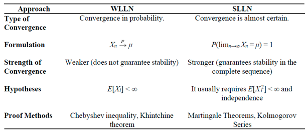
2.1.1. The Weak Law of Large Numbers (WLLN)
Let {Xi}i≥1 be a sequence of independent and identically distributed random variables with finite expected value E[Xi] = μ. Then, the sample mean:
converges in probability to μ, i.e.,
We can say that the probability of the sample mean deviating from μ by an amount greater than ϵ converges to zero as the sample size increases.
As Blitzstein and Hwang (2019) point out, convergence in probability by the weak law of large numbers does not guarantee that the sequence of sample averages will eventually stabilize around μ. It only ensures that, for sufficiently large sample sizes, the averages will be close to μ with high probability. Furthermore, the WLLN is usually demonstrated by applying Chebyshev's Inequality or through Khintchine's Theorem, which only requires the existence of a finite expected value.
2.1.2. The Strong Law of Large Numbers (SLLN)
SLLN establishes almost certain convergence (or convergence with probability 1), which is a stronger form of convergence:
this implies that the set of results in which the sample mean does not converge to μ has zero probability.
Almost certain convergence as highlighted in SLLN implies that over an infinite number of repetitions of the experiment, almost all sequences of sample means will converge to μ. In terms of comparison, this is a much stronger statement than convergence in probability in WLLN, as it implies stability over the complete sequence of observations. To arrive at a proof of SLLN we often use Martingale Convergence Theorems or the Kolmogorov Series, for example, which require stronger assumptions, such as the existence of second-order momentum (i.e., E[Xi2] < ∞).
For the purposes of differentiation, below is a table comparing the weak law and the strong law of large numbers:

Table 1.
Comparing the strong law of large numbers with the weak law of large numbers.
2.1.3. Central Limit Theorem
As Stevenson (1981) pointed out, the Central Limit Theorem probably represents the most important concept in statistical inference. This theorem states that, under certain conditions, the sum (or mean) of a large number of independent and identically distributed (i.i.d.) random variables tends to follow a normal distribution, regardless of the original distribution of these variables.
Consider a sequence of independent and identically distributed random variables X1, X2, ..., Xn, with expected mean μ and finite variance σ2. The Central Limit Theorem states that the standardized variable:
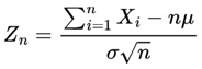
converges in distribution to a standard normal variable N(0,1) as n→∞. In mathematical notation:
As Blitzstein and Hwang (2019) highlighted, for the validity of the CLT, the following conditions are generally required:
- Independence: the variables Xi are mutually independent.
- Identically Distributed: all Xi have the same distribution with mean μ and variance σ2 < ∞.
- Finite Mean and Variance: the existence of a finite mean and variance is crucial to guarantee convergence to normality.
2.2. Monte Carlo Simulation
Simulation is an essential tool for understanding the phenomena of the world around us.
According to Fernandez-Granda (2017), Monte Carlo methods use simulation to estimate quantities that are difficult to calculate exactly. We can say that the Monte Carlo method was developed through Ulam and Metropolis (1949) as well as with significant contributions from John von Neumman, whose initial approaches began in 1946 and were later improved in the Manhattan Project and other subsequent years.
According to Kleiss (2019) Monte Carlo Simulation has been very important for scientific and industrial progress and its applications can be found in many other fields of study. According to Fernandez-Granda (2017), when we apply Monte Carlo Simulation we will also see natural convergences. As pointed out by Rajhans and Ahuja (2005), Monte Carlo simulation is characterized as a means of imitating the real world and has proved to be another case in which we can see that it has led to improvements in the industrial production process.
In the field of business administration, according to Nwafor (2023) Monte Carlo simulation is very useful in managerial decision-making processes. In the field of archaeology, McLaughlin (2023) raised the importance of adopting a more quantitative approach rather than verbal descriptions as a way of increasing precision and reducing human bias in certain activities.
When we look through the literature, we see that monte carlo simulation goes far beyond its original proposal and has a transversal character, covering basically all fields of science. In the field of computer science, Cunha Jr. et al. (2014) shows that parallelizing the Monte Carlo method in cloud computing environments, using the MapReduce paradigm, offers an efficient solution to overcome the method's computational limitations in complex simulations, thus reducing the time required as well as the processing cost.
Moreover, the results of Guatelli and Incerti (2017), show us the applicability of this technique to the field of medical physics by assisting in the decision-making process for the treatment of tumors in patients. Through Favaloro (1990) we can see that monte carlo simulation has been used to assess the variability in measurements made from angiograms and thus estimate the uncertainty associated with these variations, for example.
In addition to the micro world, Monte Carlo simulation is also very influential in the macro world, especially in helping scientists study the behavior of the universe, as presented by Trotta (2008) and Baratta et al. (2023).
2.3. Analysis of Duplicate Data in a Random Draw with Replacement and Uniform Distribution
2.3.1. Birthday Problem and Stirling Numbers
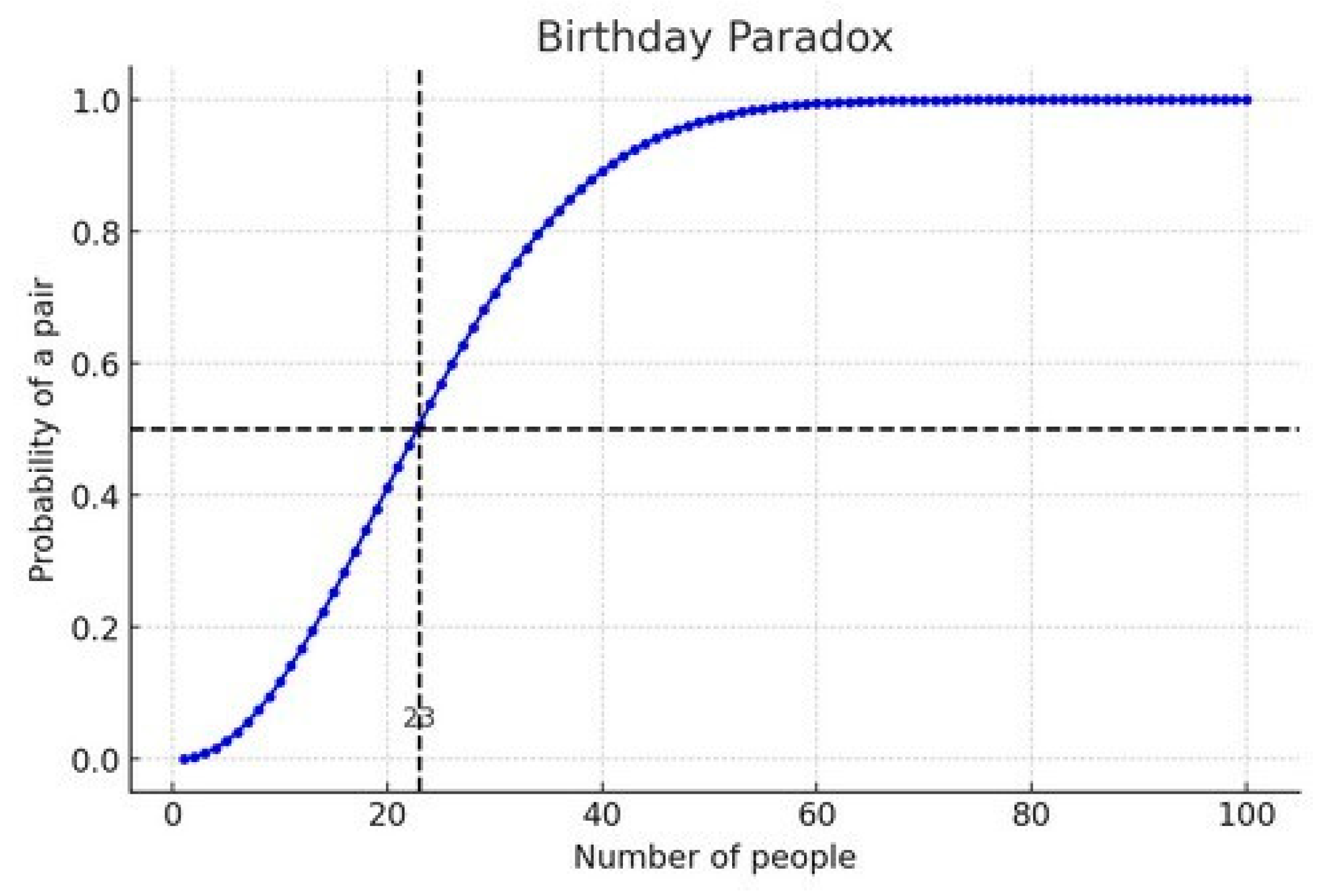
The birthday problem is one of the best-known paradoxes within the field of statistics due to its counterintuitive results for the human mind. This paradox asks: how many people do we need to put together in a group so that the probability of two of them having a birthday on the same day is greater than 50%?
Well, below is one of the best-known formulations for dealing with this paradox:
When we apply the formula, the answer is somewhat surprising, since with only 23 people, the probability of at least two people having a birthday on the same day already exceeds 50%. This probability increases considerably as the number of people in the group grows, as we can see in the figure below.
Figure 2.
Graphical analysis of the birthday paradox.
The authors Yancey (2010), Mihailescu and Nita (2021), when dealing with the birthday paradox, are some of the examples of the connection between the Birthday Paradox and both first and second order Stirling Numbers to analyze the probability of occurrence of one or more conicidences of elements within a given set.
By delving into the topics of Stirling numbers, whether they are First Order or Second Order, we can be able to realize how powerful this set of techniques is for the field of mathematics and statistics and that, according to the authors Bagui and Mehra (2024), it is incredibly little debated within this universe of numbers. Likewise, through this paper, I hope to contribute to the propagation of this technique, which could be even more useful for new approaches in the field of studies on random variables and convergences in probability.
According to Riedel (2024), when dealing with scenarios in which we want to know the number of duplicate values in a list, we can simply apply the linearity of expectation and Stirling numbers, as shown below:
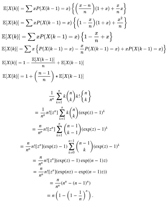
When dealing with Stirling numbers in duplicate data, we can see that if we only consider a sample of n = 100 numbers drawn with replacement, we will see that the numbers of duplicate data/values in a list will naturally converge to approximately 63.2%. This value becomes closer and closer as we increase our range of numbers drawn between a and b considering a uniform distribution.
2.4. On the Randomness Field
2.4.1. A Brief Historical Context and Its Meaning
Girolamo Cardano (1501-1574), through his paper written around 1526 and published posthumously in 1663, entitled “Liber de Ludo Aleae” which, translated into English, “The Book on Games of Chance”, took the first steps in the field of Probability Theory as a field of study.
After detailed analyses of various types of games of chance, Cardano translated by Sydney Gould (1965) developed and documented in his seminal work a systematization of probability calculations, highlighting the importance and influence of sampling on results as well as being one of the pioneers to raise the concept of expected value. As it was the Renaissance at the time, Cardano also left some reflections on the nature of uncertainty and its impact on human life and the world around us.
According to Chaparro (2023), in the field of studies on statistics and randomness, Jakob Bernoulli and Abraham de Moivre can be highlighted as having had the most outstanding work in the 18th century. Regarding Jakob Bernoulli - Swiss and the first mathematician in the Bernoulli family - we can mention that his main contributions came from his work entitled Ars Conjectandi “The Art of Conjecturing” (1713), which contains his theorizations on permutations and combinations, as well as establishing the central idea of Bernoulli's Law of Large Numbers and making it clear how he viewed probability through relative frequency, that is, if we repeat an experiment several times, the relative frequency of an event tends to approach the real probability of the event.
With regard to Abraham de Moivre (1738), who was a French mathematician who, in his paper entitled “The Doctrine of Chance” and especially its 1756 version, provided the academic community with the concept of statistical independence. As pointed out by Chaparro (2023), Moivre's other valuable contribution to Probability was through his other work entitled Miscellanea Analytica (1730). With this 1730 work, de Moivre deepens and expands concepts pioneered by Pascal and Fermat in 1654 among his famous letters, his main contributions being the first versions of what later became known as the Central Limit Theorem, on which Laplace (1810) continued this work, Binomial Approximation, as well as practical applications of probability calculus exploring concepts such as mathematical expectation aimed at games of chance as well as estimates of population parameters.
We can see that these aforementioned works were a great start in terms of mathematically formalizing the field of Probability Theory studies as well as randomness itself.
As Costa (2023) pointed out, the concept of “randomness” is too complex and all- encompassing. This is probably due, according to Chaparro (2023), to the fact that the study of randomness as a separate scientific field is relatively recent. However, in general, we consider something random to be anything that refers to the lack of pattern or predictability in an event or result. It is the characteristic of something that occurs by chance, without an apparent deterministic cause. In his study, Gödel (1940) made an interesting connection between randomness and the axioms of set theory. Gödel argues that all sets are expected to be “definable”, i.e. based in some way on some structure or rules. The problem arises from the fact that if all sets are definable, then the notion of randomness becomes empty, since something truly random could not follow a finite rule.
It is common to confuse and even use as synonyms the word “randomness” and random processes (also called stochastic processes). As we saw earlier, randomness refers to unpredictability as something general in its individual scope, a single event, while random processes are commonly related to a sequence of random events over a period of time t given a probability distribution.
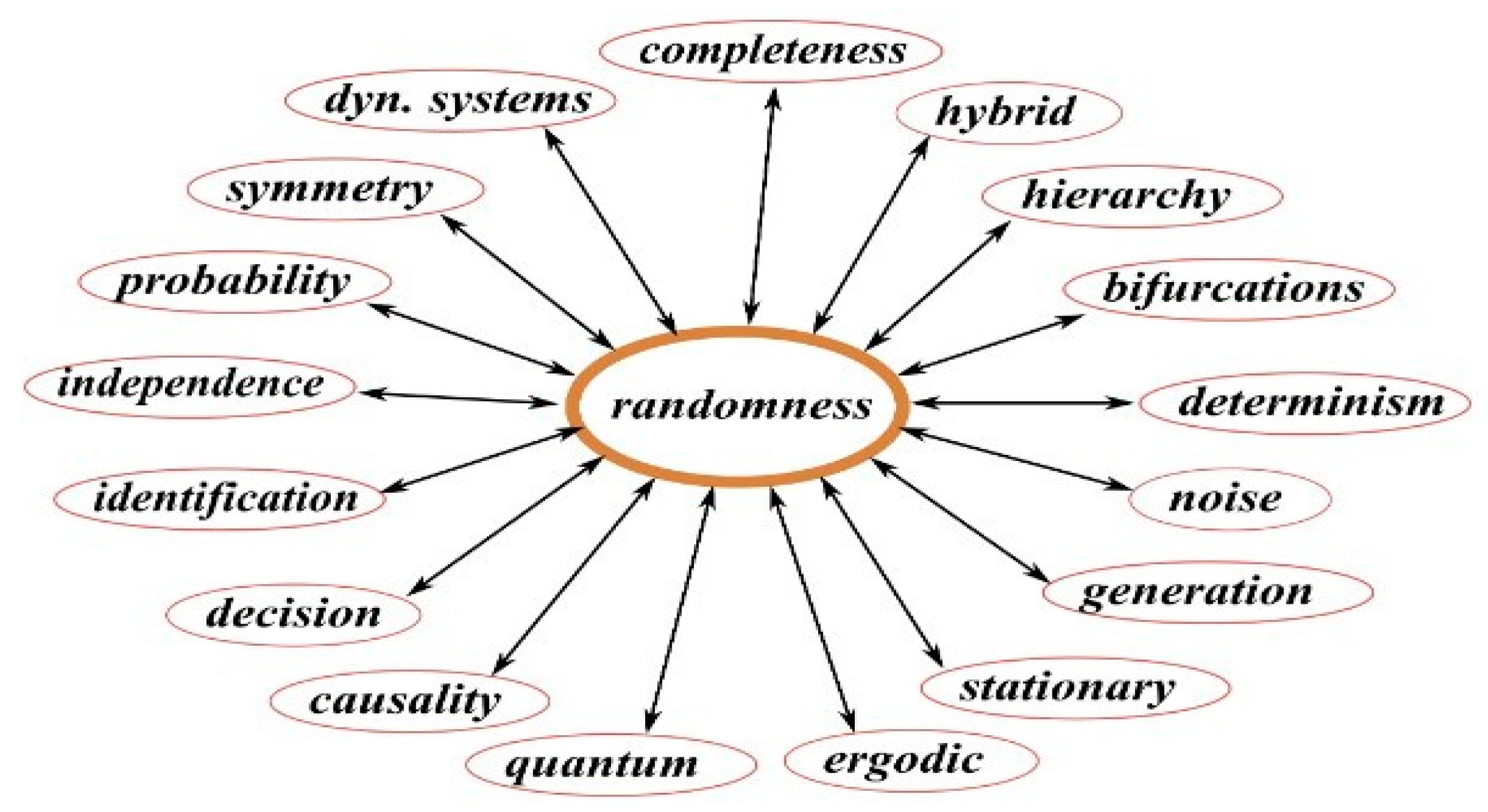
As you can see from the image, according to Costa (2023) within the field of study of randomness we can come across various other areas ranging from probability theory to dynamic systems and quantum physics. Therefore, we can infer that randomness is an interdisciplinary field, not only remaining within its core as it is usually related to statistics, mathematics and physics, but also being an integral part and/or of discussions in apparently “more distant” areas, such as Biological Sciences, Philosophy and Theology, for example.
Figure 3.
Ramifications of the field of study of randomness by Costa (2023).
Due to its scope, it is common for questions to arise within this field of study about the true nature of randomness, especially in theology and philosophy when addressing issues related to free will. Could randomness be completely random or is the randomness we consider purely due to our ignorance of all the variables that permeate the world and universe we know?
According to Chaparro (2023), these thoughts began to emerge in ancient times through philosophers such as Democritus, who firmly believed human beings consider something random simply because they are unaware of the universe and all its particularities as a whole. On the other hand, Aristotle raised the idea nature has patterns that could in no way have been part of chance alone.
Moving on to a time not so long ago, Albert Einstein also coined a well-known phrase in academic circles, stating that “God doesn't play dice” when referring to the probable non- existence of true randomness in the natural world.
The physicist Henri Poincaré, in his work “Science and Method” (1908), dedicated a chapter just to dealing with the profound complexity of chance/randomness and, according to the visions and studies shared by him, randomness is nothing more than the measurement of the ignorance of human beings.
As also discussed, Kucharski (2016) highlighted Poincaré's 3 degrees of ignorance, the first degree of ignorance being the act of knowing all the information about the variables behind a phenomenon considered random, so we could be fully able to represent mathematically through calculations what the expected final results could be, just as with established physical laws, for example.
In the second degree of ignorance, Poincaré makes us reflect even if we understand the laws that govern the universe, our ability to predict the future of an object is limited by two main factors: not knowing the exact initial states and the limitations of measurements. This means that no matter how precise our measuring instruments are, there will always be a degree of uncertainty about the initial state of an object.
This uncertainty, however small, can amplify over time, making future forecasts increasingly inaccurate, and this, for example, is easily verifiable and measurable through the Lyapunov time scale, which states that there is a time lapse in which a system becomes chaotic, that is, until the level of entropy increases considerably to the point of making any kind of long- term forecasting difficult.
Finally, the third degree of ignorance refers to the fact that we don't know the initial conditions or the physical laws behind the observed phenomena.
In addition, the field of study in Complex Dynamical Systems, according to Knill (2019) and corroborated by Akter and Ahmed (2019) aims to identify patterns through order in chaos (a deterministic system that is unpredictable) and the mathematical modeling of systems in motion in order to identify their behavior and make predictions of phenomena, whether physical, biological or financial, for example, as well as understanding the limitations of such predictions and their impacts.
These ideas about the possibility of the existence of “degrees of determinism” in the universe are also corroborated by Machicao (2018) and Costa (2023).
De Jouvenel (2017) shares a little about the myth of Cassandra and Oedipus as a form of representation of the deterministic world. Both share a central theme: the powerlessness of human beings in the face of fate. Both characters were aware of the future, but were unable to prevent it from being fulfilled. While Cassandra is an example of how knowledge of the future does not guarantee control over it, Oedipus illustrates how trying to avoid fate can lead to its fulfillment.
Normally, supporters of the “Deterministic School” such as neuroscientist Sapolsky (2023), apply arguments similar to those mentioned by Aristotle and Democritus and, in recent years, with the development of the field of study of Dynamic Systems, more specifically on the subfield called Chaos Theory, whose pioneers were Henri Poincaré (1854-1912) and Edward Lorenz (1917-2008) there are “patterns” that are present in nature that are undeniably fascinating both in mathematical and visual terms.
Other examples that can corroborate the thesis of the Deterministic School are the so- called Fractals. A Fractal, a word that comes from the Latin “Fractus” referring to something “broken” or “fragmented”, was first coined by Mandelbrot (1977). We can say that fractals are geometric patterns that present a repetitive pattern, what we can call “self-similarity”, which occur naturally, on different scales or not, in various phenomena from nature to art. We can see that, in particular, the property of self-similarity makes objects visually complex and fascinating.
We can say that there are several properties besides the remarkable self-similarity that make up a fractal, among which we can mention the main ones:
- Fractal dimension: while Euclidean geometric objects (lines, planes, solids) have integer dimensions (1, 2, 3...) fractals, on the other hand, have a “fractal dimension” which is a fractional number;
- Infinite Complexity: Fractals have infinite complexity, since their details can be repeated on smaller and smaller scales, i.e. by enlarging a small part of a fractal, we will always find new details and patterns;
- Irregularity: Fractals are generally irregular and do not follow Euclidean geometry;
- Self-organization: Many fractals can arise through simple processes of self-organization, in which patterns can occur through a set of rules;
- Scale invariance: in addition to self-similarity, some fractals can also have statistical scale invariance, i.e. their basic statistical properties can remain the same at different scales.
Furstenberg (2014) highlighted some of these aforementioned characteristics, especially by emphasizing the importance of “zooming in’’ on fractals to understand their properties in which this process of repeated magnification reveals the intricate self-similar patterns that characterize fractals. In addition, he highlights the significance of fractal dimension, which is a key concept in understanding the complexity of fractals. In his paper we can see that he suggests this dimension is closely linked to the study of ergodic averages in dynamical systems.
With regard to the presence of fractals and their properties in nature, we can easily give some examples such as snowflakes, river bends, lightning during a storm, in which, like branches of a tree, we can observe a series of repetitive patterns and ramifications similar to the “general structure”. Furthermore, in some flowers, plants and vegetables we can notice a pattern of self- similarity, such as Romanesco Broccoli, Succulents and Black spleenwort, for example, which we can see in the figure below by Barnsley (2014) to the right of the so-called mandelbrot set.
Figure 4.
Mandelbrot Set (1977) by Diehl et al. (2024) and Black Spleenwort by Barnsley (2014).

In order not to deviate from the main focus, which is to address randomness, issues related to Fractals as well as the field of Dynamical Systems itself can be further explored through some references such as Knill (2019), Machicao (2017), Barnsley (2014), Goufo et al. (2021), Diehl et al. (2024) and Youvan (2024), the latter four references addressing the concept of self-similarity and fractals with more emphasis. For a more in-depth look at ergodic theory, we recommend the paper by Viana and Oliveira (2014).
Another important point commonly discussed in the Deterministic School is the concept of self-organization. We say that self-organization is the ability of a complex system to structure itself without the need for external intervention or a predefined plan. In other words, self- organization occurs when the components of a system interact with each other and, through these interactions, patterns and structures emerge.
Sumpter (2005) argues that, despite the apparent complexity of many collective behaviours, such as the formation of shoals, flocks of birds or ant colonies, there are relatively simple principles that can explain their organization. The author also points out that simple mathematical models, based on these rules of interaction, can reproduce many of the patterns observed in real collective behaviors.
Although it doesn't have a well-defined name in the bibliographies, we can also mention the “School of Indeterminism”, which has a completely opposite approach to that of the Deterministic School, whose central idea is based on the principle that everything around us is governed purely by random factors, therefore, it is a game in which we cannot win, that is, by non-controllable and unpredictable factors. We can also say that among the main examples in which this approach is very present is through Quantum Physics and Quantum Computing.
Naturally, this school of thought is directly linked to the concept of the existence of free will. One of its proponents is the neuroscientist Nicolelis (2020) who noted that the brain shows electrical signals and/or readiness potential around 500 milliseconds before a voluntary movement takes place. At first glance, this seems to suggest that the brain “decides” before the person is aware of the decision. Despite this, the author states that there is not enough evidence since free will may have manifested itself before or during this process, even if the electrical activity precedes the physical movement.
We can also say about the possibility of a “Hybrid School” of thought in which it aims to unify parts of what we know about the universe being deterministic at the same time as free will is present in human beings.
2.4.2. Intuitions of Mises-Wald-Church
As pointed out by Terwijn (2016) and corroborated by Blando (2024), one of the first attempts to conceptualize the term Randomness mathematically was through von Mises (1919). We can say that it was von Mises who introduced the intuition that randomness must be something unpredictable. As such, he proposed a concept called Kollektiv to refer to an infinite sequence of events that satisfies certain statistical properties.
Of the two main features of the Kollektiv, we can say that the first is based on the central idea of the Law of Large Numbers, in which the relative frequencies of different events must converge on limit values. The second, however, is based on the idea that betting systems are impossible, i.e. it is hoped that there is no system that will allow someone to predict the next results with sufficient accuracy to guarantee a long-term gain. The latter is strongly related to the basis of the Efficient Markets Hypothesis, a theorization put forward by Fama (1998) that revolutionized the way investors and economists view the financial market.
A short time later, two other authors, Wald (1936) and Church (1940), also made important contributions to thinking about how we define randomness. Wald (1936) tried to analyze randomness from the point of view of random sequences as models and thus developed statistical methods for testing hypotheses by verifying, for example, whether a sequence was generated by a random process or whether there might be some underlying structure. Church (1940) revised and extended von Mises' theory by mentioning the concept of countable sets and recursive theory to rigorously formalize randomness, while at the same time being an important intuition for the emerging field of computing, above all by defining randomness from the perspective of algorithmic complexity.
As argued by Terwijn (2016, p. 5) “we thus arrive at the notion of Mises-Wald-Church randomness, defined as the set of Kollektiv's based on computable selection rules”. Thus, the concept of randomness as something unpredictable was derived through the intuitions of Mises- Wald-Church, and was therefore all too important for the progress of Randomness Theory in the following years.
2.4.3. From Absolute Randomness to Algorithmic Randomness
2.4.3.1. Kurt Gödel’s Incompleteness Theorems
Gödel's Incompleteness Theorems (1931) whose work was translated from German into English by Bauer-Mengelberg (1965) establishes two fundamental theorems. The first states that in any sufficiently powerful formal system, such as Peano's Arithmetic, there are propositions that are true but cannot be proved within that system. Therefore, we can say not all mathematical truths are accessible through axiomatic methods. The second theorem complements the first by saying that a consistent formal system cannot prove its own consistency.
We can say that, according Wolfram (2002) and corroborated by Terwijn (2016), Gödel's theory of Incompleteness (1931) was an important basis for the theory of computability as well as the theory of automata and the theory of complexity.
This connection to Gödel's work is strongly linked to the field of studying randomness, for example, due to the fact that the modeling of chaotic systems cannot be completely described and/or predicted. In this sense, systems that involve randomness can contain behaviors whose origin is not entirely deducible.
Furthermore, the idea that some logical sequences cannot be deduced refers to a type of logical randomness, as explored by Chaitin (1969) and (1975) in his theory of algorithmic complexity. In this sense, Gödel's Incompleteness Theorems (1931) show a form of fundamental limitation in mathematical knowledge, since they demonstrate that there are truths that cannot be proven within consistent formal systems. This limitation can be seen as a kind of “structural uncertainty” in the very foundations of mathematics, since not all truths are accessible by axiomatic methods. This perspective has implications both for formal logic and for computability theory and the modeling of complex systems.
2.4.3.2. Borel's Absolutely Normal Numbers and Alan Turing's Approach
We know that Alan Turing's focus was on the principles of computing, more specifically, intelligent systems. However, due to his strong interest in the field of cryptography, he was inevitably led to delve into the nature of randomness. According to Downey (2017), Turing became interested in the paper published by Emile Borel (1909) and the concept of normality.
As well documented by Downey (2017), Borel (1909) in his studies on the Law of Large Numbers arrived, among other results, at the so-called absolutely normal numbers. Formally, we can say that a number x is absolutely normal if, in any base b, each digit d in the set 0, 1, ..., b-1 appears with frequency exactly 1/b throughout the infinite expansion of the number.
As a classic example originating from the Copeland-Erdos theorem (1946), if we consider a base 10, each digit between 0 and 9 must appear with a frequency of exactly 10% in the decimal expansion. Therefore, for example, the combination of two digits such as “12” or “34” must appear with a frequency of 1% and so on.
Copeland-Erdös (1946), motivated by the papers of Borel (1909) and Champernowne (1933), showed that the sequence 0.p1p2p3,..., where pi is the i-th prime, is normal in base 10. This means that concatenating, in sequence, all the prime numbers expressed in decimal base generates a normal number that we can call the Copeland-Erdös constant, let's see:
0.2357111317192329313741…
In terms of cardinality, we can say that the set of absolutely normal numbers is “almost” the set of all real numbers. This means that if we choose a real number “at random”, the chance of it being absolutely normal is 1, i.e. it is practically certain that it will be absolutely normal. Despite its near certainty, proving that a number will be absolutely normal is too complex a task. This is because the definition of absolute normality is very demanding: it needs to apply to all bases, not just one specific base. It would be necessary to analyze the behavior of its expansions in all bases, which is a very complex task in both mathematical and computational terms.
From now on, as Downey (2017) rightly points out, instead of dealing with the metaphysical essence of absolute randomness, we will analyze randomness from now on through different levels and angles.
According to Downey (2017), Turing states that in mid-1938, in one of his many unpublished papers during his lifetime, he suggested an apparent connection between absolutely normal numbers and computable numbers. Turing (1936) states that a computable number is one whose decimals can be calculated by finite means, such as by a Turing machine or any other equivalent computational model.
The core idea is that the numbers we commonly use in mathematics are not just computable, but their computability might be a pathway to constructing normal numbers. Turing seems to be suggesting that the very process of computing a number’s digits could be a method for generating a normal number. We can say that this is a significant connection because explicitly constructing normal numbers is a difficult problem.
According to Downey (2017) and Becher (2012) Turing in his unpublished work “A Note on Normal Numbers” even proposed a theorem and proof for absolutely normal computable numbers. However, a few years later, in 1997, some disconnected points were found and, therefore, at first his proof was not fully accepted until Becher, Figueira and Picci (2007) reconstructed the model keeping Turing's original ideas and came to the conclusion that despite the fact of some disconnected points in the proof presented, Turing was right in his modeling thus confirming the existence of absolutely normal computable numbers.
2.4.3.3. Martingales
According to Terwjin (2016), an alternative way of formalizing the notion of unpredictability of an infinite sequence called martingale was presented by Ville (1939). We can say that a martingale is defined as a stochastic process X = (Xt)t∈T adapted to a filtration (Ft)t∈T, where T is a set of indices (usually discrete or continuous time), which satisfies the following conditions:
Integrability: ∀ t∈T, E[|Xt|] < ∞.
Martingale property: ∀ s, t ∈ T with s < t,
E[Xt | Fs] = Xs almost surely.
The martingale property means that, given knowledge of the past up to time s, the best prediction for the value of X at future time t is its current value Xs. In other words, there is no way to ‘predict the future’ of the martingale process based on the information available.
As presented above, Ville (1939) showed that the non-existence of an indefinitely growing martingale is equivalent to Kolmogorov's classical definition of probability, providing a basis for sequential statistical tests and probabilistic inference.
A classic example of a martingale is a symmetrical random walk on a discrete number line. Let Xn be a sequence of random variables representing the position of a player in a fair bet game. If in each round the player wins +1 with probability 0.50 and loses -1 with probability 0.50, then the sequence Xn, defined as the cumulative sum of these independent increments, forms a martingale with respect to the natural filtering Fn, because the conditional expectation of the future position, given the past history, is always equal to the current position:
E[Xn+1∣Fn] = Xn.
In addition to Ville (1939), Doob (1953) was another very important mathematician in the development of fundamental results, such as the martingale convergence theorem. Despite its strong relationship with the concept of randomness, we can see that there are some fundamental differences with the so-called martingales.
On the one hand, randomness is a broad concept that encompasses any process whose evolution over time is governed by uncertainty, and which may exhibit statistical trends, directional fluctuations or chaotic behavior. In contrast, a martingale is a specific stochastic process that satisfies the property that the conditional expectation of the next value, given the available history, is equal to the present value, implying the absence of a systematic upward or downward trend.
So, while randomness can manifest itself in a variety of formats, including processes with ‘bias’ or autocorrelation, a martingale represents a restricted subset of random processes in which, under a suitable probabilistic model, the best predictor for the future is always the current state, making it fundamental in probability theory. In summary, we can say that every martingale is random, but not every random process is a martingale.
Some of the areas where martingales are applied include finance through option pricing, statistics with sequential tests and physics through random walks, Brownian motion and superstring theory, for example.
2.4.3.4. Martin-Löf Randomness
As Terwijn (2016) pointed out, Martin-Löf's (1966) approach dealt with randomness from the perspective of classical probability theory and measurement theory.
In this sense, Martin-Löf (1966) proposed that an infinite sequence of bits S = s1, s2, s3, …, sn is considered random if it cannot be identified as non-random by any effective test of randomness.
A randomization test is a sequence of measurable subsets of the space of all bit sequences {0,1}∞, defined by
where each Un is a set of measure 2-n, representing subsets where the sequence is not random at an increasing level of precision. If a sequence belongs to all these Un sets, it is considered non-random.
U1⊇U2⊇U3⊇… Un
The Martin-Löf universal test can be seen as the “most powerful possible test” of randomness, because it encompasses all conceivable randomness tests that are computationally enumerable.
An S sequence is random in the Martin-Löf sense if it does not belong to the intersection
 where Un is an effectively describable set with measure 2-n.
We say that these tests are related to the compressibility of the sequence by Turing machines, that is, if an infinite sequence S can be described by a short program, it is not random. If no compressed description is possible other than the sequence itself, S is random.
Martin-Löf's theorizing was surely one of the great revolutions in thinking about true randomness and in the deliberate search for how to measure it. In the following years, we saw the development of a set of statistical tests of randomness such as the Diehard test by Marsaglia (1996) and the battery of tests proposed by the National Institute of Standards and Technology, NIST, for example.
2.4.3.5. Algorithmic Randomness and Kolmogorov Complexity
The paper entitled “Grundbegriffe der Wahrscheinlichkeitsrechnung” by Andrey Kolmogorov (1933), translated into English as “Foundations of the Theory of Probability”, we can say was a milestone in the formalization of probability theory since Kolmogorov established the rigorous foundations of probability theory using an axiomatic approach based on David Hilbert's set theory and Lebesgue's integrals.
As we can see from Blitzstein and Hwang (2019), Kolmogorov defined probability as a function P that satisfies three main axioms:
- (1)
- P(A) ≥ 0 for all A⊂S
- (2)
- P(S) = 1
- (3)
- If A ∩ B = ∅,
Then (A∪ B) = P(A) + P(B).
In addition to the axiomatization of probability, we can also see that Kolmogorov in his seminal paper defined the concept of probability space, which consists of a sample space, i.e. the set of all possible outcomes of an experiment. He also defined an algebra of events, i.e. a set of subsets of the sample space, as well as a probability measure, which refers to a function that assigns probabilities to events.
Another notable contribution is the use of measure theory as a way of making it possible to deal with continuous probabilities and events with zero probability, which until then had not been possible using the classical approach to probability. For these reasons, Andrey Kolmogorov is often recognized as the “Father of Modern Probability Theory”.
We can say that the field of algorithmic randomness is a field of study that seeks to define and quantify the concept of randomness in data sequences. Unlike traditional probabilistic approaches which are based on statistical measures and probabilities, algorithmic randomness focuses on the inherent complexity of sequences. In short, algorithmic randomness can be defined in terms of computability and algorithms. Normally, this concept tends to become clearer when we talk about Kolmogorov Complexity. With regard to this concept, as Terwijn (2016) pointed out, it may be more appropriate to consider at least three authors: Kolmogorov (1965), Solomonoff (1964) and Chaitin, all of whom have made significant contributions to this seminal field of study.
Kolmogorov (1965) in his study provided the academic community with a model for quantifying a sequence of data. As Vadhan (2012) highlighted the Kolmgorov Complexity refers to the length of the shortest program, in a universal programming language, that generates a specific sequence that we called it as string. The Kolmogorov Complexity can be defined as:
where U is a universal Turing machine, an |p| is the length of the program p.
K(s) = min {|p| : U(p) = s}
We can that say there are two key properties: random strings and structured strings. We say a string s is considered structured when there are obvious patterns and, consequently, they are less complex and can be described using a short program.
Let's consider the following string s1 = 01010101010101010101. You can see that there is a clear pattern in this binary sequence - the repetition of “01”. In a compact program, we could easily write “write 01” and “repeat 10 times”.
On the other hand, a random string s is one that satisfies the following condition K(s) ≈ |s| in which, according to Campani and Menezes (2001), it is not possible to extract an obvious pattern in a given sequence of data by means of a Turing machine. Let's consider the following string s2 = 10110100101011010001. We can see that there is no obvious pattern that can be easily identified, so we can say that it has a higher level of Kolmogorov complexity than sequences that have some kind of pattern throughout the sequence.
In fact, not every string is comprehensible, which means that a random string has a Kolmogorov complexity close to its original size. This theorizing in the successful attempt to measure the level of randomness and compressibility of systems was very relevant to the field of studies on true randomness and, above all, to information theory.
2.4.3.6. Hardness vs Randomness
A few years later, another seminal paper in the field of algorithmic randomness and computational complexity entitled “Hardness vs Randomness” presented by Nisan and Wigderson (1994) explores the relationship between the difficulty of solving computational problems, i.e. “hardness”, and the ability to generate pseudo-random numbers efficiently, i.e. “randomness”.
The authors demonstrate that, under the assumption of the existence of computationally difficult functions, it is possible to construct efficient pseudo-random generators that reduce or eliminate the need for genuine randomness in probabilistic algorithms. This result establishes a relevant theoretical connection in the field of complexity class studies, suggesting that if sufficiently “hard” functions exist, then BPP = P.
The main implication of this paper lies in the possibility of transforming random problems into deterministic ones. Therefore, we can say that this paper was a major turning point for the development of optimization techniques as well as, among other examples, a more mature way of creating and accepting certain pseudo-random number generator algorithms (PRNGs) as an integral part for simulation and cryptography purposes.
The field of complexity theory usually unites the fields of computer science and pure mathematics. In this sense, it is often studied from different angles. As one of the most recent examples in the timeline, Vega (2022), Vega (2024), in addition to having worked continuously on the proof of P = NP in other manuscripts, has also contributed to advances in studies on Robin's divisibility criterion and other inherent topics to present a formulation for the proof of the Riemann Hypothesis.
2.5. From Entropy, Algorithmic Randomness to Structure in Randomness
The deliberate search for patterns and better measurement of randomness has always been the subject of curiosity and study over the years. However, we will only focus on the topics that have stood out the most.
The concept of entropy initially arose with the second law of thermodynamics through the German physicist Rudolf Clausius (1822-1888) in the mid-19th century, around 1865.
Clausius realized that the energy in a system is not completely converted into useful work, but there is always a portion that is lost in the form of heat. This energy “lost” or unavailable to do work was what he called entropy. Furthermore, the second law of thermodynamics states that the entropy of an isolated system, i.e. one with no exchange of energy with the outside world, tends to increase over time, i.e. disorder increases. To further his work, Clausius (1879) gave us his mechanical theory of heat.
Although this concept initially came from “pure physics”, it opened the door to the development and better understanding of many other academic areas, from statistical physics to information theory and cryptography, for example.
Shannon Entropy is a very relevant concept for the field of Information Theory. Its formulation was originated by Shannon (1948) through his work entitled “A Mathematical Theory of Information”.
Shannon entropy is a fundamental measure of the uncertainty or randomness associated with a random variable. In the context of Information Theory, it quantifies the average amount of information needed to describe an event or message. Mathematically, Shannon entropy is defined as the expected value of the negative of the logarithm of the probability of each possible outcome of the random variable. The higher the entropy, the greater the uncertainty or randomness of the system, and vice versa.
Below, we see its formulation:
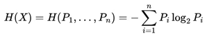
Pi = Pr(X = xi).
A few decades later, Pincus (1991) took another major innovative step in the field of statistics with the so-called Approximate Entropy (ApEn), which is a statistical technique used to quantify the regularity and unpredictability of fluctuations in time series data. ApEn is, for example, particularly useful for analyzing non-linear and non-stationary data, where traditional methods of analysis may be inadequate.
This seminal study by Pincus (1991) inspired many studies in different areas of knowledge. As an example, we can mention Delgado-Bonal (2019) through his study with notable results in the field of the financial market and his approach of using Approximate Entropy (ApEn) as a way of measuring randomness and identifying patterns in the stock market. Below is some of what he described about Approximate Entropy:
“In this regard, Approximate Entropy (ApEn) is a statistical measure of the level of randomness of a data series which is based on counting patterns and their repetitions. Low levels of this statistic indicate the existence of many repeated patterns, and high values indicate randomness and unpredictability. Even though ApEn was originally developed after the entropy concept of Information Theory1 for physiological research2, it has been used in different fields from psychology3 to finance4”(Delgado-Bonal, 2019, p.1).
Mageed and Bhat (2022) revisited classical entropies such as Shannon's, Rényi (1961) and Tsallis (1988) and introduced the Generalized Z-Entropy (GZE), which is a generalization that includes these entropies as special cases. In addition, they discussed how the fractal dimension measures the complexity of patterns such as coastlines or Koch's snowflake and how it can be derived from entropies. The authors demonstrated that GZE offers a unified framework for studying fractal systems through generalized entropies, concluding that GZE is an important tool for exploring complex and fractal systems, paving the way for future applications in interdisciplinary areas.
Tao (2007) discusses the decomposition of combinatorial objects into three fundamental components: a structured (dominant) component, a pseudo-random component and a residual error term.
This approach has proved to be innovative and not restricted to the field of pure mathematics, as it allows predictable patterns to be isolated from chaotic elements, facilitating the analysis and resolution of problems involving large data sets with unspecified structures, and is therefore also an important contribution to the field of algorithmic complexity studies.
We can see that this approach by Tao (2007) was one of the notable studies on randomness from the perspective of combinatorial analysis. As such, it has influenced new studies such as the one carried out by Trevisan et al. (2009) when analyzing the relationship between high entropy distributions and efficiently sampled distributions, for example.
Blum and Blum (2022) propose an innovative approach to understanding consciousness based on the pillars of theoretical computer science, using tools from computational complexity theory and machine learning. The authors introduced a concept called the Conscious Turing Machine (CTM), that is, an abstract computational model inspired by the Turing Machine and the work of neuroscientist Baars (1997), but aimed at exploring consciousness through a formal machine model for consciousness. The structure of the CTM is shown below:
Figure 5.
The Conscious Turing Machine Structure by Blum and Blum (2024).
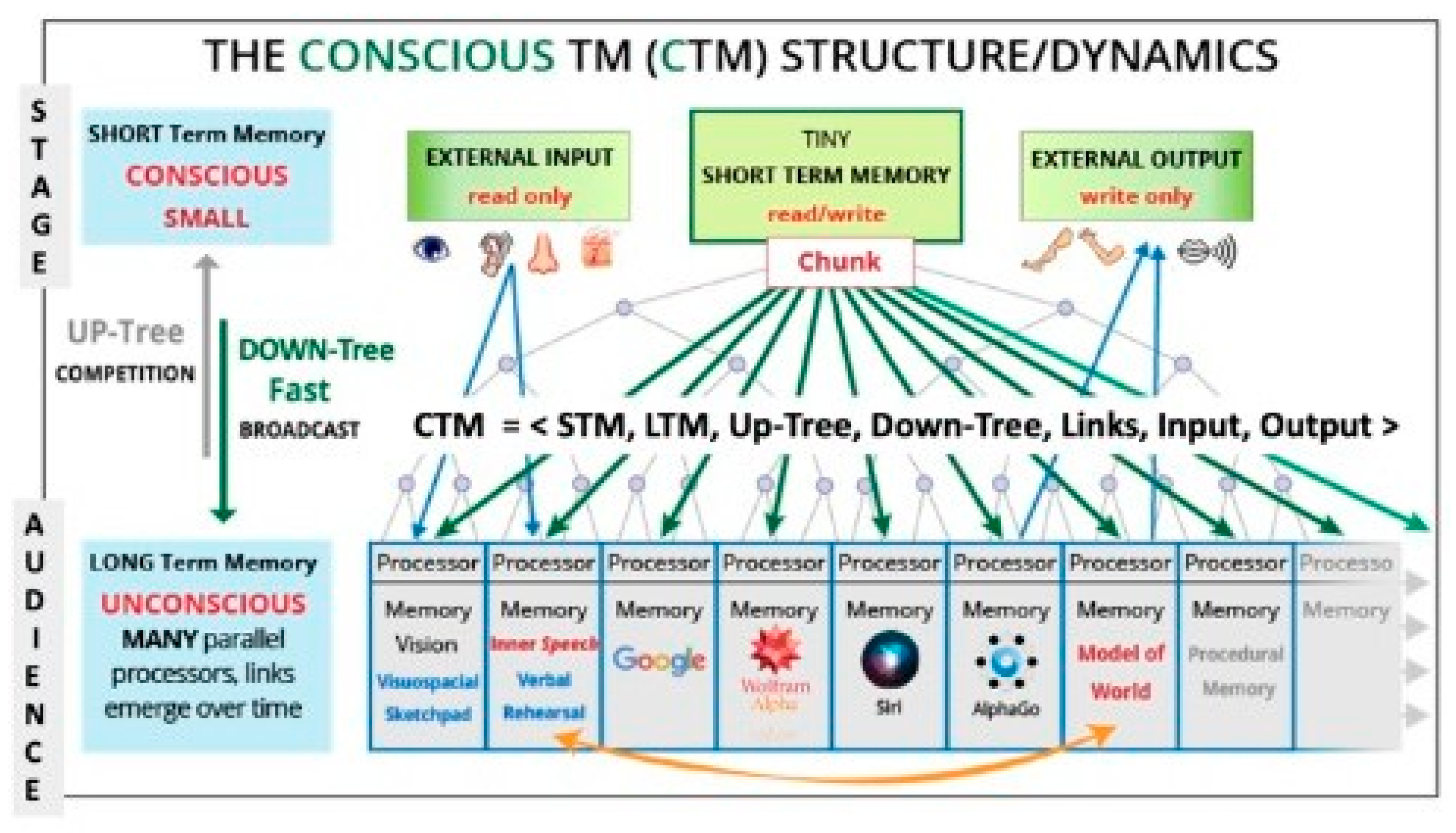
Furthermore, Blum and Blum (2024) in their most recent study in this direction concluded that consciousness in artificial intelligence will not only be possible, but also inevitable. The aim of these theorizations is to demonstrate how this perspective of theoretical computer science can contribute to research into consciousness and to encourage further studies in this direction.
2.6. Types of Random Number Generators: PRNG, Quasi-RNG, TRNG, QRNG
Informally, we say that an algorithm refers to any set of well-defined steps that leads to a certain end result. According to Cormen et al. (2022) an algorithm - in computing terms - can be defined as a computational procedure that uses a value or set of values as input, which in turn goes through an intermediate processing step that generates a value or set of values as output. An algorithm is usually designed to solve some computational problem. In this sense, as Baeza- Yates (1995) pointed out, algorithms are at the heart of computer science.
According to L'Ecuyer (2017) who was one of the authors of a relevant PRNG algorithm through Panneton et al. (2006), although they don't formally exist in the way we know them today, so-called random number generators and their role of providing “justice” and therefore serving as a means of decision-making and choice have always been present in people's lives since ancient times through other means such as through a coin and 6-sided dice, as we can read below:
“The Romans already had a simple method to generate (approximately) independent random bits. Flipping a coin to choose between two outcomes was then known as “navia aut caput”, which means “boat or head” (their coins had a ship on one side and the emperor’s head on the other). Dice were invented much earlier that that: some 5000-years ones have been found in Iraq and Iran”(L’Ecuyer, 2017, p.2).
Galton (1890) was one of the notable examples of scientists who used the 6-sided cubic dice as a tool in his research. As a result, he designed a method to sample a given probability distribution:
“He used cubic dice (with six faces) but after throwing the dice he was picking up each die by hand and placing it aligned in front of him, eyes closed, and considered the orientation of the upper face. This gives 24 possible outcomes per die (almost 4.6 random bits)”(L’Ecuyer, 2017, p.2).
In more recent times, we can say that the first RNG algorithm came from John von Neumann (1946) through the middle-square method (1951). For a more in-depth timeline on the history of Random Number Generators, we recommend following the paper by L'Ecuyer (2017).
Within the world of random number generators, we can say that there are 4 main branches: Pseudo-Random Number Generators (PRNGs); Quasi-Random Number Generators (QuasiRNGs); Truly Random Number Generators (TRNGs) and, more recently, taking into account concepts from quantum physics, Quantum Random Number Generators (QRNGs).
2.6.1. Pseudorandom Number Generators (PRNGs) e Quasi-Random Number Generators (Quasi-RNGs)
Bhattacharjee and Das (2022) argued that pseudo-random number generators (PRNGs) are a type of deterministic generator, i.e. derived from a mathematical function whose outputs appear to be random. According to Babaei and Farhadi (2011) it is desirable for PRNG algorithms to statistically satisfy certain requirements in order to be considered good, for example we can mention: uniform distribution, independence, large period and unpredictability.
We can also say that there are two main categories: Non-congruential and Congruential PRNG algorithms.
Figure 6.
“Types of PRNGs” by the author.
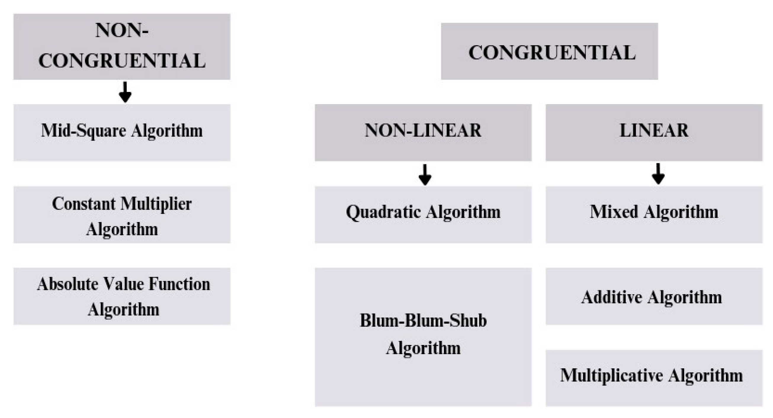
We say that a PRNG is congruent when it relies on a modular congruence relationship to generate the next sequence of numbers. A classic example of an algorithm with this structure is the LCG (Linear Congruential Generator) or DH Lehmer PRNG, which was one of the pioneering algorithms and therefore inspired the creation of many similar ones over time. Its formulation is shown below:
where:
Xn+1 = (a * xn + c) mod m
Xn+1 = next number of the sequence
Xn = the current number a = the multiplier
c = the increment m = is the modulus
mod = modulo operation.
It is common for there to be many models and algorithmic proposals, some of which may be better than others depending on the user's objectives. In this sense, like Machicao (2017), it is common to see scientific publications addressing the quality of PRNGs, as recently demonstrated by Boutsioukis (2023) in his article comparing models known as the Mersenne Twister by Matsumoto and Nishimura (1998), the Middle Square Method by John Von Neumann (1946) and the Linear Congruential Generator (LCG) by DH Lehmer and Thomson and Rotenberg (1958).
As Stinson (2005) points out we must emphasize although most pseudo-random algorithms are not the most suitable for the field of cryptography, there are some mathematical models of PRNGs that have historically been considered very good for information security, such as Blum-Blum-Shub by Blum et al. (1986) and Fortuna by Schneier and Ferguson (2003).
Although a pseudo-random function (PRF) is not exactly a PRNG due to some subtle differences that can be better explored through Vadhan (2012), we can say that the Naor and Reingold (1997) algorithm also has a strong structure for possible cryptographic applications.
Nowadays, we can mention some very promising new PRNGs in this field involving information security, such as Itamaracá PRNG by Pereira (2022) due to its results in statistical tests as well as the fact that its design employs the absolute value function as a form of "mirroring", making it even more difficult for someone malicious to take the path back and discover the initial seeds.
In addition, Itamaracá has been pointed out by Levina et al. (2022) and corroborated by Aslam and Arif (2024) because it is considered simple and practical, as well as because it generates aperiodic sequences, i.e. without having a cycle ending moment at first. In this sense, repetition will occur if and only if the values of the 3 initial seeds happen to appear in the middle of the sequence in exactly the same order, which, in probabilistic terms, will basically make it unlikely/impossible for a cycle to occur with repetition as we increase the maximum value of the interval and a uniform distribution.
Below, we can see the Itamaracá PRNG formulation:
As fixed parameters, we have:
M ∈ℝ+: a maximum positive value, representing the upper limit of the scale of the numbers generated.
λ∈ℝ+: a positive multiplicative constant whose values must be very close to 2 (1.97, 1.9886, 1.99545...).
As initial values, we have:
s1, s2, and s3 ∈ℝ+: three starting numbers called seeds, needed to start the random sequence.
As derived variables, or intermediate process ip, we have:
and the generated sequence can be represented by:
Δs : s3 – s1
xn : or nth pseudorandom number generated.
At each iteration n, the pseudo-random number xn is generated by the formula:
Δs = s3 – s1
s′1 = s2, s′2 = s3, s′3 = xn.
It is common that, due to the deterministic nature and the fragility that may exist in some PRNG algorithms, some scientists over time come to propose improved solutions to these classical models, such as the one proposed by Rahimov (2011), Widynski's “Squares” (2020) and the method of Padányi and Herendi (2022) with all of these with the proposal to improve the model of the Mean Square Method, proposed by John von Neumman (1946).
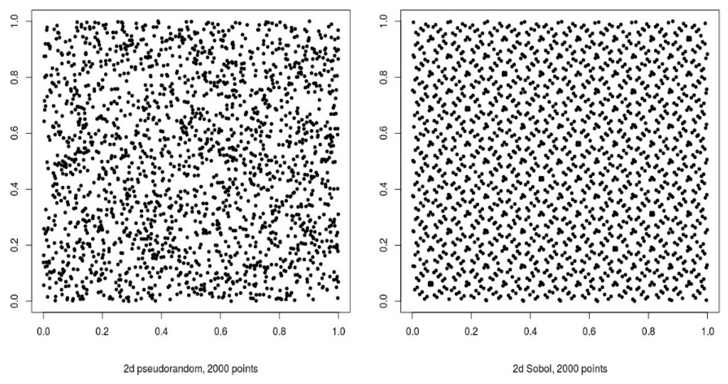
Quasi-RNGs, which stand for Quasi-Random Number Generators, are also deterministic in nature and very similar to PRNGs. However, according to Dutang and Wuertz (2009) and corroborated by Smith et al. (2017) the focus of Quasi-RNGs is more on creating a model that tries as much as possible to make each random number output equally (rather than approximately) distributed within the intervals considered.
Figure 7.
Bivariate uniform samples - pseudorandom (left) and quasirandom (right) Smith et al. (2017).
Figure 7.
Bivariate uniform samples - pseudorandom (left) and quasirandom (right) Smith et al. (2017).
It should be clear and understandable that pseudo-random number generators (PRNGs), despite their great relevance, are actually part of a larger scope of topics entitled “Pseudorandomness”. Due to its inherent particularities and rich extension, we see from Vadhan (2012) that other points are also important, such as the computational model and complexity classes, randomness extractors, expander graphs, list-decodable codes, derandomization techniques, among other topics. As such, this field of study should be seen as a separate field, deserving its own discipline for study.
2.6.2. True Random Number Generators (TRNGs), Quantum Random Number Generators (QRNGs) and Quantum Techniques
We also have TRNGs (Truly Random Number Generators) which, according to Herrero- Collantes and Garcia-Escartin (2016) are those designed to produce unique and unpredictable random sequences that normally use natural sources such as atmospheric noise and radioactive decay, for example. Sunar et al. (2006) presented their theoretical and practical approaches to a TRNG that has withstood adversarial attacks.
More recently, we have the so-called QRNGs, an acronym for Quantum Random Number Generators, which we can also say are part of the TRNG category, however, due to some particularities within quantum physics, it is preferable to classify them as a separate category.
As we can see from Herrero-Collantes and Garcia-Escartin (2016), Quantum Random Number Generators (QRNGs) exploit quantum mechanics phenomena to generate genuine random numbers. On the quantum mechanics, Avigliano (2014) explores the intersection of Rydberg atoms and superconducting cavities, focusing on manipulating and controlling these systems for quantum information processing. Uria et al. (2020) presented an innovative protocol to deterministically prepare a Fock state of a large number of photons in the electromagnetic field. Among these and other results, quantum algorithms can be developed over time that exploit the power of quantum computing to solve problems usually linked to optimization issues in different areas of knowledge, including cryptography, artificial intelligence and medicine.
Among the two main forms of QRNGs are those designed from the perspective of quantum optics (i.e. single photon emission, quantum interference, polarization of photons, understanding of light states, among others) and non-optical quantum (i.e. radioactive decay, thermal noise in electronic components, spin of subatomic particles, quantum vacuum fluctuations, among others).
Just as in the field of PRNGs TRNGs, where it is common to observe several different techniques behind their global developments, QRNGs are no different. As an example of its vast ramification, Contreras et al. (2021) introduced a robust and efficient iterative method for the reconstruction of multipartite quantum states from measurement data. The method shows fast convergence, especially in high-dimensional systems, and is applicable to any informationally complete set of generalized quantum measurements.
Furthermore, as demonstrated by the authors, its robustness against realistic errors in state preparation and measurement steps makes it a potentially valuable tool for quantum information processing and for emerging technologies such as Quantum Random Number Generators (QRNGs). This was just one of the papers included in more than 50 academic materials and publications carried out by a global project called “Quantum Random Number Generators: cheaper, faster and more secure” funded by the European Union.
Other outstanding works in this emerging field are Hensen et al. (2015) which reports a breaktrhough experiment on the Bell Inequality test, a fundamental concept in quantum mechanics that explores the nature of reality and locality. Among its main results, the data implied a statistically significant rejection of the local-realist null hypothesis, so the experiment provides strong evidence against local realism, strengthening the worldview of quantum mechanics. Through this and other experiments, Abellán (2018), Amaya, and Tulli et al. (2019) idealized Quside and, with it, developed technologies to strengthen information security as well as an important step towards new “quantum level” randomness certifications.
Meng et al. (2024) developed a GD-enhanced quantum RNG based on quantum walks of single photons in a linear optical system which, in addition to its good properties for uniform distributions, is also considered a flexible model for other probability distributions.
2.6.3. Other Categories of Random Number Generators
In addition to the categories mentioned above as the main ones, we can also say that there are other designs and ways of generating random numbers as well as forms of encryption for the information security area. Among these, we can highlight those derived from Chaotic Maps such as those worked on by Machicao (2018), Moysis et al. (2022) and Moysis et al. (2023).
There are some other PRNG algorithms whose design is also differentiated, such as Rule 30 developed by Wolfram (1983), whose main sources are techniques such as cellular automata, which, in turn, as also corroborated by Mariot el al. (2021), uses a set of rules similar to the so- called “Game of Life” within the field of study of mathematics with regard to evolutionary algorithms. In addition, another paper highlighted in the bibliography is that of Balková et al. (2016) who, through their studies, came up with an innovative technique for generating an aperiodic pseudo-random sequence using the infinite word technique.
2.1. Uniform Distribution
We can say the uniform distribution is one of the main probability distributions in statistics, especially when it comes to the field of study of random variables. The authors Blitzstein and Hwang (2019) state this distribution assumes each element within an interval (a, b) has the same probability of occurrence, so we can say within this interval we can expect sequences of random numbers.
Below, for example, is the probability density function (PDF) of the uniform distribution for continuous values:
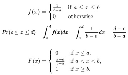
The expected value for a continuous uniform distribution is:
And its respective variance:
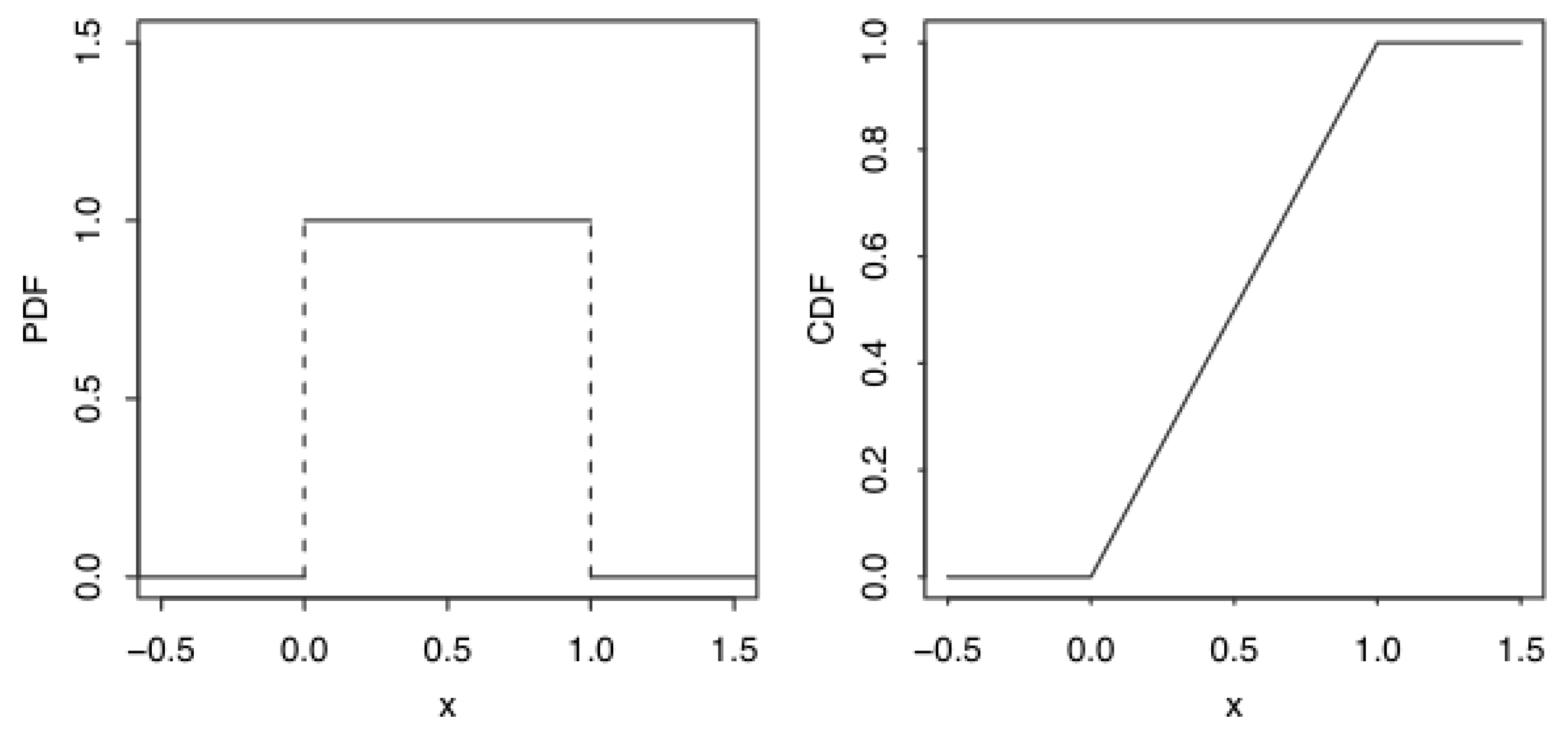
The PDF (Probability Density Function) represents the “density” of probability at each point in the interval. In the uniform distribution, the PDF is constant throughout the interval, indicating the probability of any value occurring within that interval is the same.
The CDF (Cumulative Distribution Function) of a uniform distribution can be said to increase linearly from 0 to 1 in the interval [a, b]. This means the cumulative probability grows proportionally as x moves from a to b.
Figure 8.
PDF and CDF graphical analysis by Blitzstein and Hwang (2019).
2.1. Compound Interest
As Campolieti and Makarov (2018) point out, compound interest is a way of calculating the interest on an investment or loan, where the interest for one period is added to the initial principal balance, and in the following periods, interest is calculated on this new total value (initial principal balance + accumulated interest). By this definition, and as also noted by Smart and Zutter (2020), it is “interest-on-interest” growing exponentially over time.
The following is the formulation of compound interest usually presented in financial mathematics bibliographies:
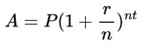
A = Final amount, resulting from the sum of the initial principal balance and Interest
P = Initial principal balance
r = interest rate, which must be on the same time basis as the period
n = number of times interest applied per period
t = number of time periods elapsed
Through Stojkovic et al. (2018) and Karn et al. (2024) we see that compound interest has always been a topic of debate throughout history by various mathematicians, from the studies of Jakob Bernoulli, Leon John Napier, and Leonhard Euler to the present day.
Nowadays, compound interest continues to be explored in various fields, including actuarial sciences, economic sciences, and even more specific areas like Computer Science through machine learning algorithms and algorithmic complexity. As Bartlett (1993) pointed out, it is also relevant in biology, where it is used to study population growth, from bacterial cultures to animal populations, and demographic growth. We can also observe this exponential behavior through Ma (2020) in his approach to dealing with epidemic scenarios as well as in Seshaiyer et al. (2020) when addressing the importance and limitations of mathematical models to model covid-19.
2.9. Sports Betting Universe
2.9.1. Understanding the Basics
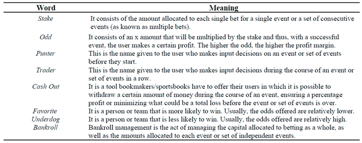
Within the world of sports betting, there are often very specific expressions inherent to this environment. Below we will look at the meaning of some of the most popular ones, which will be essential for a better understanding of this study.
Table 2.
Some basic concepts within the world of sports betting.
2.9.2. Sports Trading Market
According to Etuk et al. (2022) the world of sports betting has grown exponentially in recent years and reached the mark of more than 30,000 companies around the world with business models based on sports betting in 2019. In the same year, this market exceeded more than US$ 200 billion.
As Harris (2024) pointed out, through the repeal of the Professional and Amateur Sports Protection Act in 2018, sports betting was legalized and more than half of the states in the united states were covered by this law. According to the author, this field opens up new business opportunities and jobs, but also new challenges, both in terms of the illegality of certain platforms and the impact of betting on people's lives, especially in virtual environments. In this sense, it is necessary for government bodies, the academic community, and society as a whole to be in dialogue to debate this new business model that is here to stay.
2.9.3. The Mathematics Behind Sports Betting
2.9.3.1. Understanding Odds
The so-called “odds” refer to the probability of an event occurring. They are usually published by bookmakers (or sportsbooks, in a more modern term) in fractional or decimal form (which will be the focus of this study). As pointed out by Sladić and Tabak (2018), odds estimations by sportsbooks are carried out by experts who, in addition to relying on robust data structures, also factor in subjective analysis.
Table 3.
Probabilities of an event occurring in decimal representation by Buchdahl (2003).
| Decimal Odds | Probability | Decimal Odds | Probability |
|---|---|---|---|
| 1.1 | 0.91 | 3.25 | 0.31 |
| 1.11 | 0.9 | 3.4 | 0.29 |
| 1.13 | 0.89 | 3.5 | 0.29 |
| 1.14 | 0.88 | 3.6 | 0.28 |
| 1.15 | 0.87 | 3.75 | 0.27 |
| 1.17 | 0.86 | 3.8 | 0.26 |
| 1.18 | 0.85 | 4 | 0.25 |
| 1.2 | 0.83 | 4.33 | 0.23 |
| 1.22 | 0.82 | 4.5 | 0.22 |
| 1.25 | 0.8 | 5 | 0.2 |
| 1.3 | 0.77 | 5.5 | 0.18 |
| 1.33 | 0.75 | 6 | 0.17 |
| 1.44 | 0.69 | 6.5 | 0.15 |
| 1.5 | 0.67 | 7 | 0.14 |
| 1.53 | 0.65 | 7.5 | 0.13 |
| 1.57 | 0.64 | 8 | 0.13 |
| 1.62 | 0.62 | 8.5 | 0.12 |
| 1.67 | 0.6 | 9 | 0.11 |
| 1.73 | 0.58 | 9.5 | 0.11 |
| 1.8 | 0.56 | 10 | 0.1 |
| 1.83 | 0.55 | 11 | 0.09 |
| 1.9 | 0.53 | 12 | 0.08 |
| 1.91 | 0.52 | 13 | 0.08 |
| 2 | 0.5 | 15 | 0.07 |
| 2.1 | 0.48 | 17 | 0.06 |
| 2.2 | 0.45 | 21 | 0.05 |
| 2.25 | 0.44 | 26 | 0.04 |
| 2.38 | 0.42 | 34 | 0.03 |
| 2.5 | 0.4 | 51 | 0.02 |
| 2.62 | 0.38 | 67 | 0.01 |
| 2.88 | 0.35 | 151 | 0.01 |
| 3 | 0.33 | 201 | 0.01 |
| 3.2 | 0.31 | 501 | 0 |
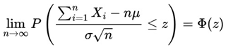
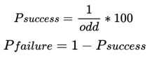
As we can see from the table above, as the multiplicative values of the odds increase, the probability of success of the event also decreases. The probabilities of success and failure for an event can be determined using the following formulas:
2.9.3.2. Calculating the Odds
According to Buchdahl (2003), if we consider that a bettor enters a sporting event with an odd of 1.80, this means we can expect approximately 55.56% chances of success and 44.44% chances of failure. If this bettor places a stake of $10 he would recover his “investment” while making a further $8 profit if the event in question ended positively, thus totaling $18.
Considering that a bettor enters a sporting event with an odd of 1.25, this means we can expect approximately an 80% chance of success and a 20% chance of failure. Therefore, if this bettor places a stake of $10, in addition to recovering his “investment”, preferably saying “risk”, since if he loses the bet he loses all his money, of $10 he will make a profit of $2.50 if the event has a positive outcome in the end, leaving a result of $12.50.
Now, let's consider another scenario in which a bettor enters a sporting event with an odd of 2.5, which means we can expect approximately a 40% chance of success and a 60% chance of failure. Therefore, if this bettor places a stake of $10 in the event that he wins the bet, he will be able to recover the amount he already had and make a profit of $15, thus totaling a positive amount of $25.
2.9.3.3. Historically, Mathematics and Statistics Have Always Been in Favor of the House
It must be clear and understandable to each of us that the business model of sportsbooks, casinos, lotteries, among other gambling variations, is completely based on the main bibliographic bases within the field of mathematics and statistics. Among the main topics we could say that it is common to use Risk Management, Return on Investment, Rates, Break-even Point, Strong and Weak Law of Large Numbers, Time Series Analysis, Expected Value, Probability, Probability Distributions, Clustering, among others, for example.
In the field of sports betting, it is common for sportsbooks to adopt a “fee” containing a percentage can range from 2% to 5%, i.e. regardless of the outcome of the market, the sportbook will always be collecting a percentage of the bettor's profit.
Furthermore, in addition to the so-called administrative fees, another common tactic used by sportsbooks is “juice” or “vigorish”, which consists of offering odds with “unbalanced” values, i.e. not in line with the real probabilities of occurrence, usually most of the time with small percentages of less, but enough, combining with the law of large numbers to make it extremely difficult for a bettor to be mathematically profitable in the long term.
As a basic example, if a database indicates that a future event should have an odd of 1.70, in order to represent reality, bookmakers will probably offer a lower odd of 1.66, for example.
Although this is relative and varies from bookmaker to bookmaker and their respective business models, it is usually common for this additional profit margin to range from 3% to 7% on so- called juice.
In addition to administrative fees, unbalanced odds through juice, statistics itself through the strong and weak law of large numbers strongly influence the player to have a negative expected value in the long term and, at best, to reach the break-even point, i.e. no profits or losses.
Let's assume that the odds offered by bookmakers for sporting events, whether soccer, volleyball, basketball or any other sport, are “considered fair” and therefore represent the same odds in real life. Let's also assume the bettor would like to place 100 consecutive bets on events with the same fixed odds of 1.25, i.e. we can expect a probability of success of 80% and 20% of failure. Let's also assume that $10 was the amount set by the bettor to be the value of each of the 100 stakes.
When we apply the odds calculation formula, we know in each event with a positive final result, the bettor will make a real profit of $2.50. On the other hand, we also know that in events with a negative final result, the bettor will lose all the money placed on the bet, in this case -$10.
In 100 independent events with equal probability, we can expect a result converging to
~80%, so we can consider that the bettor will have 80 events with a positive final result and 20 events with a negative final result.
Putting it into the formula we would get,
Positive Final Result = 2.50*80 = $200 and,
Final Negative Result = 10*20 = -$200.
So we can see that, mathematically, the bettor will at best not win or lose after a sequence of games chosen after setting the odds and the entry price/stake.
Probabilistic forces will act regardless, whether through low odds, as in the example above, or through high odds, usually those above 1.80 or 2.00 according to “professional sports bettors”.
2.10. Is It Possible to Beat the House?
The world of gambling and the idea of using a random system that is “fair” according to the Laws of Probability, according to Matheson (2021), has existed since ancient times and is mentioned in Greek mythology when he mentions Zeus, Hades, and Poseidon, for example, divided the heavens, the seas and the underworld through games of chance. Similar references can also be found in religious records, such as the Old and New Testaments of the Bible.
We can see the whole system that preceded the creation and sophistication over time of games of chance present in casinos and bookmakers is very old and shows us the concept of chance has always been, in a way, a form of entertainment and a means of decision-making for human beings.
Another point to highlight is the human quest to explore games of chance in search of consistent patterns that can allow us to predict to some degree the next results of the sequence, either through statistics or by applying concepts from physics.
When it comes to “Beating the House” or among other similar variations, first of all, what should be clear to each of us is the meaning behind these expressions. Although in general it is more commonly related to the world of betting, we can say the “house” is a well-established system and breaking it is basically unquestionable and/or unlikely or very difficult in terms of probability. We can also say the “House” can come to represent:
A System: evaluation system; labor market; physical, statistical, mathematical, biological, political, social, economic system.
An Institution: school, company, organization, governments (i.e. dictatorial regimes)
An Obstacle: a barrier that needs to be overcome
A Symbol: a reference to the status quo.
As we saw above, in summary, we can also say “Beating the House” symbolizes breaking away from something pre-established, overcoming challenges and crossing an unexplored frontier.
The deliberate quest by scientists to beat the house goes much further than financial results, but rather to identify consistent patterns and understand to some extent the true nature of randomness, which in turn has a cross-cutting nature covering several fields of science, including mathematics, statistics and physics.
In this sense, throughout history it has been common for many physicists, mathematicians and statisticians to undertake studies in order to better understand and even establish a system that is capable of beating the house. Scientists such as Henri Poincaré (1854-1912), John von Neumann (1903-1957), Richard Feynman (1918-1988), Stephen Hawking (1942-2018) and Albert Einstein (1879-1955) have also told us about their attempts to better understand and beat roulette, for example.
With regard to the question: Is it possible to beat the house in gambling and sports betting? Well, the answer is yes. However, there are some particularities and limitations that must be observed by bettors, as we will see later in this study.
2.10.1. Roulette
Throughout history, in roulette, for example, many scientists and researchers have spent hours and hours observing generated sequences and accumulating a robust database for analysis. Although many statistical concepts were already well-established, such as the Law of Large Numbers, the idea of independent events, expected value, among others, many continued to defy these natural laws in this deliberate search to identify patterns.
We can say that to this day, those groups of scientists who set out to try to beat roulette purely through observation and looking for some statistical loophole, have probably provided the academic community with even more data proving the already well-established concepts, but probably with no solid practical results in terms of making a consistent profit against the house.
On the other hand, some scientists have chosen to theorize about beating the house based on the premise of studying randomness itself through physics. According to Poundstone (2010), at the end of the 1950s, a student called Edward Thorp, observing a game of roulette, hypothesized that the existence of a possible flaw in the roulette wheel's structure could imply that the ball tended to fall in certain places. Even though Edward Thorp considered the roulette wheel to be perfect and without any flaws, he still maintained his position that the laws of physics could cause the ball to land in certain places.
Shortly afterwards, Claude Shannon (1916-2001), known for his seminal contributions to the field of Information Theory, began working with Edward Thorp to continue the theories Thorp had raised about the physics and randomness involved in roulette. The result, according to Thorp (1984) and Thorp (1998), was the creation of the first wearable computer - an analog device the size of a cigarette pack - which allowed them to obtain a return of over 44% on the roulette wheel.
According to Kucharski (2016) and corroborated by Small and Tse (2012) another notable event of scientists using physics to beat the Casino through roulette took place between 1977 and 1978 through Doyne Farmer, Norman Packard and other colleagues whose group called themselves “Eudaemons” who aimed to use their knowledge combined with a hidden computer to consistently beat roulette over the long run.
In the 1990s in Spain, Gonzalo García Pelayo, who had dedicated his career to music and film, ventured into the world of casinos and, with the help of his son Iván García Pelayo and many other family members, decided to beat the house with roulette. According to García-Pelayo and García-Pelayo (2003) and as also presented by Pfeifer et al. (2017), at first his method was more intuitive than mathematical, which consisted of checking which roulette wheels within a casino might be fouled by some kind of physical fault. The type of fault didn't matter to them either, but in the long term, after a large number of spins by the dealer, they used a data analysis exercise to analyze which groups of numbers and their respective “boxes” could contain some kind of fault and, as a result, more numbers than the average and their respective expected standard deviation.
It is known that it is normal for fluctuations around the average to occur, even in the long term. Therefore, they basically adopted the idea of the frequentist school by continuously checking whether those patterns would continue to repeat themselves in another thousand spins of the roulette wheel. As a result, Pelayo and his family came to the conclusion that certain roulette wheels were in fact statistically biased and thus favored certain groups of numbers more than others. Because of this small advantage for them, according to public sources it is known that Gonzalo García Pelayo and his family have amassed a fortune of more than 250 million pesetas in casinos in Spain and other parts of the world.
In the 21st century, a notable contribution was made by Strzalko et al. (2009) when they demonstrated the real possibility of beating the house by applying the concepts of physics and consequently addressed what is understood by mechanized randomness and how it approaches random processes.
A short time later, the authors Small and Tse (2012) also considered roulette to be a deterministic dynamic system, so if we knew how the roulette wheel worked, the mass of the ball, its initial position and calculated its acceleration and velocity, we could predict exactly where the ball would land, giving us the prize.
Figure 9.
Small and Tse’s Model.
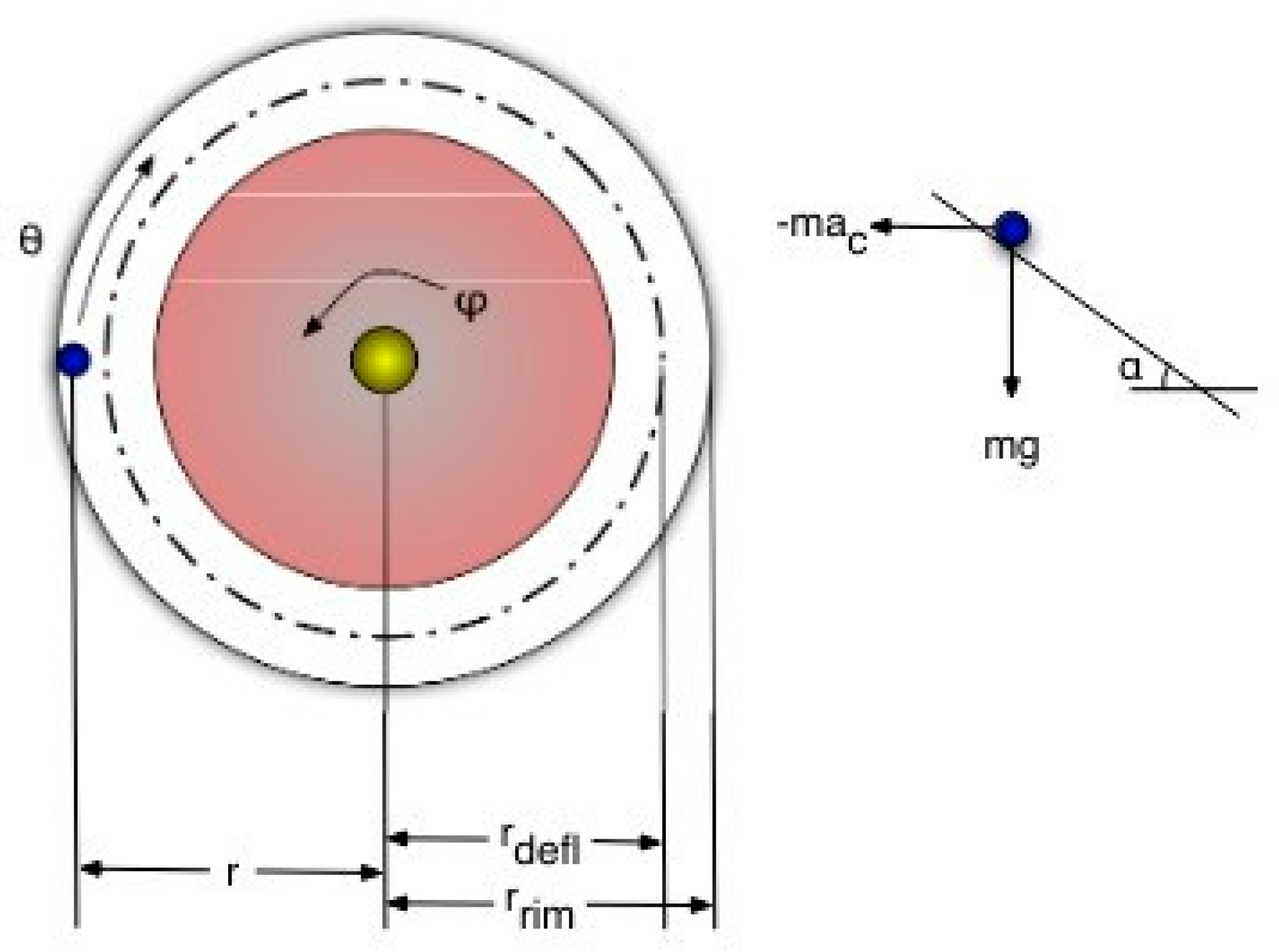
The results of the model proposed by Small and Tse (2012) showed us that roulette and its randomness is, to a certain extent, fully predictable. In their experiments, they showed us that the expected return on a random bet jumped from -2.7% to 18% in the long run.
In fact, although the results are surprising in the field of Statistical Physics when dealing with Dynamic Systems, putting them into practice in a Casino would be difficult, as it would require a lot of equipment and data to account for the sequences generated, as well as other issues such as the possibility of Casinos not authorizing the entry of these players.
As Thorp (1998) and Poundstone (2010) have pointed out, when it comes to beating the house it is preferable for players to choose to stay in the game as long as they can until the Law of Large Numbers is in their favor. Small and Tse (2012) also point out even if the odds work in the player's favor, it is still a game of chance. Therefore, we can also say the player's patience in betting during long sequences as well as having a good amount of money available are factors to be considered.
2.10.2. Blackjack
According to Jensen (2014), an average Blackjack player (also known as 21) who relies solely on super bets and luck in the game naturally has a negative expected value of $4 for every $100 wagered, indicating that in the long run the player will always lose out.
In this sense, we can say academically the first notable attempts to beat the house with Blackjack came in the form of a remarkable paper by Baldwin et al. (1956) presenting an optimal strategy for players in casinos. As we can see below, “They figured that both the player and the dealer had a finite number of possible hands, the player had only up to six possible decisions to make and the dealer’s play being fixed, there had to be a optimal way to play the game” (Jensen, 2014, p. 7).
As Jensen (2014) also highlighted, the authors initially believed that instead of players having a negative expected value of $4 for every $100 wagered in the long run, this strategy would have a significantly lower negative expected value of only $0.62 for every $100 wagered.
In 1962, Edward Thorp in his work entitled “Beat the Dealer” detailed a mathematical system that allows blackjack players to gain a statistical advantage over the casino.
According to Jensen (2014) Thorp, using rigorous mathematical and statistical methods, demonstrated blackjack is not just a game of luck, but can be influenced by strategy and knowledge.
Unlike games such as Roulette which are classified as Independent Variable Games, i.e. past results do not influence future results, the game Blackjack (also known as 21) can be classified as a Dependent Variable Game since:
“The deck is not shuffled after every round of play. Once a card has been used and the play is over for that round, that card will not be used again until the cards are reshuffled and put back into play. Thus, the outcome of one round is dependent on what cards were used in the previous round”(Jensen, 2014, p. 7).
Among its main revelations are card counting techniques and betting strategies for removing certain cards and their effects on the player's expected value.
As Jensen (2014) pointed out, knowing that Blackjack is a Dependent Variable Game, as well as the positive results of the Reno/Tahoe Rule whose positive expected value for the player was 0.09%, Thorp realized that he could obtain even better results and, with a line of research in similar directions to that of Baldwin et al. (1956), he developed his so-called Basic Strategy.
In his test, instead of using a 52-card deck, Thorp opted to use a 51-card deck. Using Monte Carlo simulation on an IBM 704 computer, he tried to measure the impact that a missing card could have on the expected value, both in favor of the player and in favor of the casino.
Table 4.
Impact on odds with card removal effect.
| Effect of Card Removal* | |
|---|---|
| Card | Effect |
| 2 | 0.3875% |
| 3 | 0.4610% |
| 4 | 0.6185% |
| 5 | 0.8018% |
| 6 | 0.4553% |
| 7 | 0.2937% |
| 8 | -0.0137% |
| 9 | -0.1997% |
| 10 | -0.4932% |
| A | -0.5816% |
In his experiment, Thorp noticed that removing an Ace gave the Casino a 0.58% advantage over the players. On the other hand, for example, removing the number 3 card gave the players a .46% advantage over the Casino, as can be seen in the table above.
The publication of the articles by Baldwin et al. (1956) and Thorp (1962) had a major impact on the casino world, as groups of people made fortunes using these techniques to the point where they were banned. Casinos, previously immune to any kind of strategy, were forced to review their rules and procedures to try to neutralize card counting and other shared strategies.
2.10.3. Other Notable Blackjack Experiments
In the 1980s, according to Casey (2008), Bill Kaplan, also sometimes referred to in some media as Micky Rosa, founded a team of students and former students at the Massachusetts Institute of Technology (MIT) for the exclusive purpose of beating the house through the game of Blackjack (21), popularly known as MIT Blackjack Team. In addition to the founder, we can mention other notable participating members who played an essential role in this project, especially in the 1990s, such as JP Massar, John Chang, Jeff Ma and Mike Aponte, as some examples.
With his strong knowledge of mathematics as well as delving into the literature on techniques for winning games of chance, especially mastering card counting as developed by Ed Thorp (1966), Bill Kaplan even created a company called “Strategic Investiments, Limited Partnership” whose business model was to provide profits to investors by beating casinos. This group of students made a fortune together and were often even banned from casinos where they were identified.
As another example, in the academic world, Persi Diaconis is a mathematician recognized for his valuable papers, either alone or in collaboration, on randomness. He is also known for having worked as a professional magician for decades and therefore has a wealth of theoretical as well as practical knowledge of techniques and games such as Blackjack.
Through his experiments and in collaboration, they came up with the Bayer and Diaconis (1992) model, which became one of their best-known theorems in which they stated that 7 times is enough to shuffle the cards so that the level of randomness reaches its ideal point. The authors also concluded that less shuffling (such as 5 or 4 times) will mean that the entropy level of the system will be far from ideal, so that the position of the cards can be predictable and, on the other hand, shuffling more than 7 times will not make the cards even more “random”, on the contrary.
Although the results of Bayer and Diaconis (1992) do not necessarily imply direct possibilities of financial gain for the players, they show us once again the importance of mathematical, physical and statistical analysis applied to games.
2.10.4. Coin Toss Experiment
In his studies, when he tossed a coin into the air, Diaconis observed that it spent a little longer with its initial side facing upwards before spinning and landing on a given surface. Diaconis, Holmes and Montgomery (2007) called this phenomenon “precession” and raised the following question: could precession influence the number of heads or tails in coin tosses?
At first, at the time of the study, Diaconis et al. (2007) raised the possibility and, consequently, a theorem that precession could give a small margin of advantage to the initial side of the coin. According to their studies, this advantage would be 1%.
Below we can see the graphical and mathematical representation of precession as well as the coin tossing machine designed to follow physical laws exclusively and eliminate any human biases as much as possible.
Figure 10.
Precession by Diaconis et al. (2007).
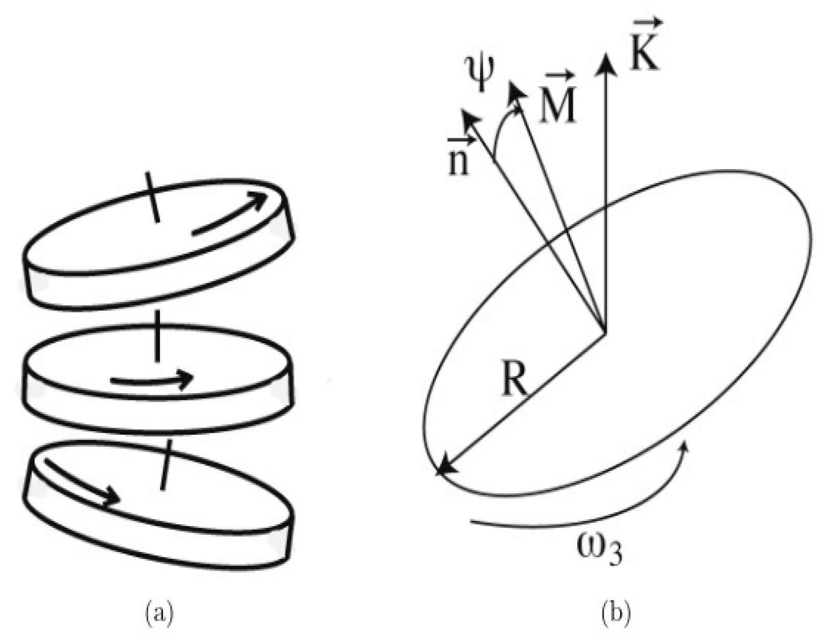
Figure 11.
Experiments by Diaconis et al. (2007).
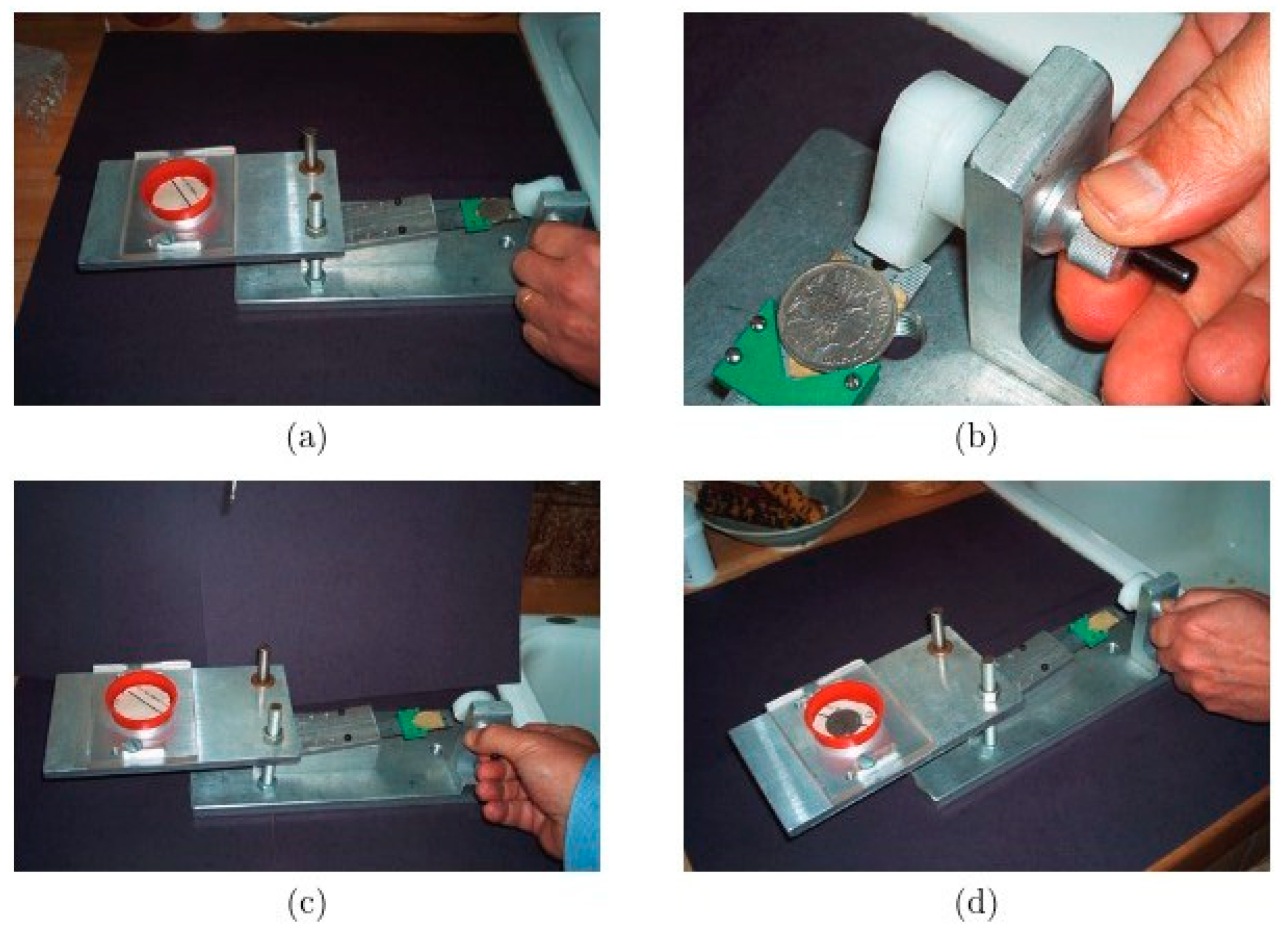
The theorem proposed by Diaconis et al. (2007) was also proven by a robust study carried out by Bartoš et al. (2023) in which they brought together a team of 48 authors who used coins minted in 46 countries in order to minimize possible biases in the research process. As a result, the authors tossed coins more than 350,757 times and the chance of the coin landing on the initial side converged to 50.8%.
The results presented by both studies were very interesting, since, despite being a result basically within the normal range expected by the law of large numbers with values converging to 50%, and this “advantage” being considered “low”, we can see the positive effects for a bettor can be better perceived in the long run, an advantage sufficient to say the player has beaten the house.
Bartoš et al. (2023) also wondered about this possible “small advantage” and its relevance in terms of the expected value for the player, which has been shown to surpass even other strategies employed in other casino games:
“The magnitude of the observed bias can be illustrated using a betting scenario. If you bet a dollar on the outcome of a coin toss (i.e., paying 1 dollar to enter, and winning either 0 or 2 dollars depending on the outcome) and repeat the bet 1,000 times, knowing the starting position of the coin toss would earn you 19 dollars on average. This is more than the casino advantage for 6 deck blackjack against an optimal-strategy player, where the casino would make 5 dollars on a comparable bet, but less than the casino advantage for single-zero roulette, where the casino would make 27 dollars on average”(Bartoš et al., 2023, p. 14).
Although the same-side bias shows small advantages for the initial side of the coin and therefore enough for the player to have a positive expected value in the long run, as Diaconis et al. (2007) point out, we can still consider the coin toss to be as close to a fair game as possible.
2.10.5. Lottery
There are many types of lottery games around the world. However, a few of the most common models prevail, such as the design lottery (49, 6, 6, t) also known as 6/49, in which the player must choose 6 numbers from a range of balls from 1 to 49 and, by combining the 6 numbers chosen with the numbers drawn, the player wins the jackpot.
Throughout history, some people, whether mathematicians by training or not, have used their knowledge of probability theory and combinatorial analysis to make fortunes in lotteries.
One notable case was Stefan Mandel - a Romanian mathematician - who, between the 1960s and 1990s, revealed and was proven by investigations by public bodies such as the CIA (Central Intelligence Agency) and FBI (Federal Bureau of Investigation), for example, that he won the lottery jackpot 50 times, 14 of which were by using a method he called “Combinatorial Condensation”.
Although Mandel never fully revealed his method, what is generally known is that he chose to play lotteries whose prize pools were considered very high and the cost/benefit ratio between the prize pool and the number of all possible tickets was always positive. It is known he initially played and won a lottery in Romania whose design was 6/49, in which he focused on making sure that at least 5 of the 6 numbers drawn were correct.
Therefore, Mandel's jackpots came from buying all possible combinations and/or removing certain sets of numbers from the ticket to reduce the number of combinations needed and at the same time “increase” the probability of winning, according to his methodology. For a more in-depth analysis of this story, we recommend consulting other sources, such as Wikipedia and the article by Stömmer (2024).
Another experiment similar to Mandel's, and also documented by Amado et al. (2019), was the story of a group of students from the Massachusetts Institute of Technology (MIT) and a couple, Jerry Selbee and Marge Selbee, from Michigan, United States. The methodology they used in the Cash Windfall was to wait for the prize to accumulate and, if there were no winners of the maximum prize, it was also divided to eventual winners of “secondary winners”, they realized that the cost-benefit ratio considering the price of the tickets as well as the purchase of all the possible combinations necessary and, adding the fact the prize could be divided to other winners who did not match all 6 numbers, the couple would always come out with a positive result.
A few years later, as pointed out by the couple via the BBC media (2022) Jerry shared a bit more about this story “Out of 18 (tickets), I won US$1,000 for a four-number winning ticket and 18 three-number winners worth about US$50 each, which is about US$900. So by spending US$1,100, I got about US$1,900 back”.
With the success that “small” winnings could mathematically constant under this methodology, Jerry and Marge created the company - GS Investment Strategies LLC - to pursue in a “professional” way the art of beating the house through the lottery. It is estimated that the couple accumulated more than 60 tons of lottery tickets and won more than 26 million dollars between 2003 and 2012, as well as engaging with several other residents of their city in this project.
Although it was a very interesting idea and its results can be proven by probability theory, its practical applicability tends to be very limited due to some factors such as: the need for a solid knowledge of mathematics and probability theory; human or software factors that may present errors during the process of filling in tickets with all possible combinations and, finally, due to the rules of lottery games that may be modified over time by increasing the unit price of each ticket and/or limiting the number of tickets purchased by each player, for example.
Nowadays, through the work of Stewart and Cushing (2023) it was shown it is possible to establish a mathematical formulation employing concepts from probability theory and combinatorial analysis that guarantees at least 2 exact combinations in a UK lottery game in which players have to choose 6 numbers ranging from 1 to 59 using only 27 different tickets.
Figure 12.
One set of 27 tickets for n = 59 using the configuration (B, C, E, E, E) by Stewart and Cushing (2023).
Figure 12.
One set of 27 tickets for n = 59 using the configuration (B, C, E, E, E) by Stewart and Cushing (2023).
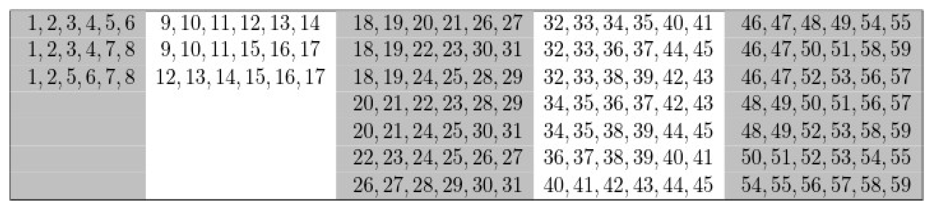
Although, in financial terms, this UK Lotto scenario is not representative and players will continue to be at a great disadvantage due to other factors such as the price of the ticket and the value of the prize, it is a paper that provides us with significant advances in terms of how statistical analysis can provide new horizons for decision-making in games of chance.
2.10.6. Financial Market
2.10.6.1. Black-Scholes-Merton Model
The Black-Scholes-Merton (BSM) formula is a mathematical model widely used in the financial market to determine the theoretical price of options and other derivatives. It was developed by Fischer Black and Myron Scholes (1973) and, through a paper written independently but with equivalent and complementary results by Robert Merton (1973).
Regarding authorship, Edward Thorp stated he had come up with a similar formulation in 1967 and had kept it secret due to the success of his investments. Polemics aside, This model marked a significant advance in the analysis of derivatives since it demonstrated that quantitative analysis can offer valuable insights beyond the intuition of the investor, which was considered very subjective and unmeasurable.
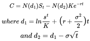
C = call option price
N = CDF of the Normal Distribution
St = Spot price of an asset
K = Strike price
r = risk-free interest rate
t = time to maturity
σ= volatility of the asset
The following are the five Greek letters related to Black-Scholes-Merton, each of which can be further explored in Yu and Xie (2013) and Paunović (2014).
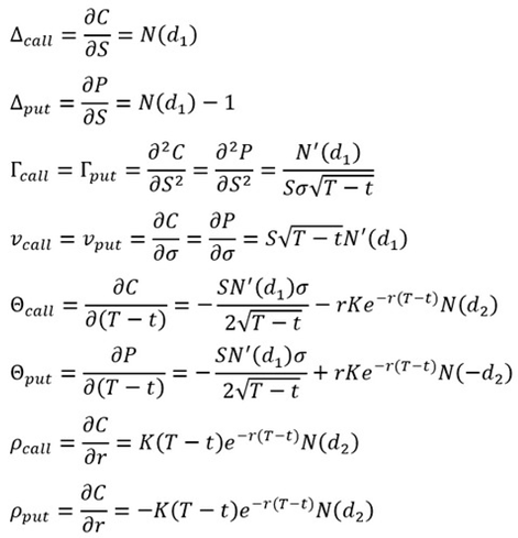
This formulation, as we can see through Joyner (2016) extends beyond its practical applications in the financial market, being more commonly noted through the field of physics with complex dynamical systems and, above all, related to thermodynamics due to the similarity with the heat equation, since both are partial differential equations (PDEs) but used in different contexts. The Black-Scholes-Merton model is also related within the field of Quantum Physics, as we can see from the studies by Accardi and Boukas (2007) and Vukovic (2015).
2.10.6.2. Kelly’s Criterion
The Kelly Criterion, developed by mathematician John Larry Kelly Jr. (1923-1965), is a well-known strategy in the field of Trading and Sports Betting since, according to Kelly Jr. (1956) and Kim (2024), it is a bankroll management technique that seeks to maximize long-term returns while minimizing the risk of losses in betting or investment situations with known probabilities.
As we can see from the image below, this criterion seeks to find the perfect balance between aggressive betting and capital conservation.
Figure 13.
Kelly’s Criteria by Kim (2024).
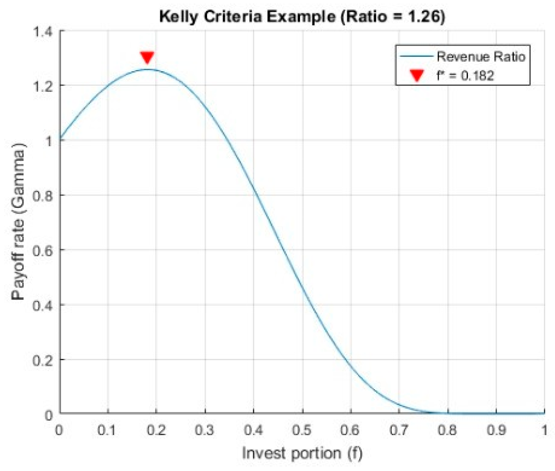
And its formulation,
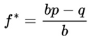
f*= the fraction (%) of the bankroll
b = Odds (as a decimal), always equal to 1
p = Winning probability
q = Losing probability, calculated 1-p
The formula allows us to determine what percentage of all our available capital is considered “optimal” to place on a single event, whether in the world of investments or betting.
Despite its valuable contributions and being one of the main references for maximizing gains and minimizing risks in investments, the Kelly Criterion has some limitations, such as the fact it was designed to work in the long term, so there is a risk of ruin in the short term. Another point to note is that, as it is based purely on probabilities, small errors in estimating probabilities can lead to significantly different results and thus compromise the capital invested.
Given these advantages and limitations, over the years it has been a strong object of study in the academic community. Thorp (2008) demonstrated that the Kelly Criterion as a means of portfolio management, together with other techniques and particular knowledge, helped him to achieve a return of more than 20% with a standard deviation of about 6% a year for 28.5 years, showing that his achievements as an investor and hedge fund manager were not just “luck” but too much asset management and, above all, mathematics. In addition to his valuable contributions to blackjack, Thorp also proved to be one of the most successful stock market investors in history.
Most recently, Baker and McHale (2013) have presented an approach that extends the Kelly Criterion with a focus on modeling uncertainty rather than the original idea based on an estimated probability. One of the main results found by the authors is that reducing the size of the investment can provide a better expected utility in the presence of such uncertainty. As real probabilities are usually uncertain, Chu et al (2018) followed the same starting point when considering uncertainty modeling and proposed in their approach an analysis of estimators such as Minimax, Bayesian and loss functions in a theoretical decision framework. In addition, Wu et al. (2015), anchored in the Kelly Criterion and the Kullback-Leibler Divergence (KL), came up with an approach that proved to be positive in which an “adaptive probability” is considered over time by analyzing the historical series of the proportion of wins (W) by the total value (W+L) instead of adopting a fixed theoretical probability.
Matej et al. (2021) analyzed the Kelly Criterion, Markowitz's Modern Portfolio Theory (1952) as well as Informal heuristics used by bettors in sports such as Horse Racing, Basketball and Soccer. Among their main results were that formal assumptions are considered the best but are impractical in many scenarios and the Fractional Kelly Criterion may be more suitable. Jacot and Mochkovitch (2023) have presented an extension of Kelly's model for mutually exclusive bets applied to horse racing. Furthermore, the study by Kim (2024) has presented a mathematical model called the Kelly Criterion Extension (KCE), an innovative approach aimed at improving the traditional capital growth function to better adjust to dynamic market conditions.
Despite the many positive aspects of the Kelly Criterion, economist Paul Samuelson (1971) raised some pertinent reservations about this method. He argued, for example, about the confusion between the concepts of time horizon and risk aversion, in which many gamblers seek other objectives besides maximizing financial gains, such as a finite time horizon, maximizing utility or minimizing the risk of ruin, which could lead to choices other than those suggested by the Kelly criterion. According to Samuelson, Von Neumann-Morgenstern's expected utility theory was a more consistent and general model for decision-making under risk. Despite these caveats, it is important to bear in mind that the Kelly Criterion is not invalidated, but should be carefully analyzed by the people concerned.
In the same way the work published by Claude Shannon (1948) in Information Theory influenced Kelly Jr. to develop his method, we can also say the Kelly Criterion was one of the great milestones for studies on the financial market as well as for other fields of science, since through a quantitative approach to stock and options market analysis it presents us with an important tool for decision theory, resource optimization, and mathematical modeling.
2.10.6.3. Jim Simons: The King of Quant
James Harris Simons (1938-1944), mathematician, cryptographer and pioneer in quantitative investing, known for the “Quant Revolution”, shaped the financial industry with his innovative and highly profitable approach. Through the founding of his company Renaissance Technologies and the Medallion Hedge Fund in 1982, Simons developed and implemented complex quantitative strategies, based on mathematical models and sophisticated algorithms, to identify patterns in the financial markets and generate consistent returns over time.
From 1988 to 2023, his investment fund “Medallion” had an average annual return of 40% after fees. It is estimated that Renaissance Technologies has generated a return of more than US$ 100 billion since it was founded. In addition, Jim Simons' net worth is estimated to have reached approximately US$ 31.8 billion. In this sense, he is considered in the financial market world to be the greatest investor in history.
Simons' approach was based on the premise that financial markets are complex systems, but that they can be modeled mathematically. His team, according to Simons (2023) was made up of world-class mathematicians, physicists, astrophysicists, statisticians and programmers, who developed sophisticated algorithms to analyze vast amounts of market data, looking for patterns and correlations that could be exploited to generate profits. In this sense, we can say it was probably one of the first practical applications of machine learning techniques in the financial market.
Due to the confidentiality contracts Jim Simons signed with his clients, little is known about what lies behind the whole Renaissance Technologies method, however, throughout history we have been given some clues such as: highly diversified strategies involving a variety of assets with “high frequency at low risk” with the aim of minimizing risks while increasing the probability of generating positive returns.
Normally, on an average day, the algorithms would execute thousands of short-term trades trying to take advantage of small price fluctuations. Another striking feature is that Simons' quantitative models were constantly updated and refined to adapt to changes in the financial markets, something that is very similar to what is required in the field of time series studies, as we can see, for example, in Giannerini and Rosa (2004), Nason (2006), Levenbach (2017), Hyndman (2018), Makridakis et al. (2018), Pereira (2022), and Petropoulos et al. (2022), in which we see a variety of mathematical models and machine learning algorithms that update their respective forecasts with the input of new data. For those belonging to the field of business management, Chopra (2004) also presents us with a solid literature covering the main points in time series analysis applied to logistics.
Jim Simons and his hedge fund is a demonstration that it is possible to overcome the Efficient Market Hypothesis (EMH), i.e. a classical and until then widely accepted approach that, like Markov's memoryless property of a stochastic process, it is basically impossible/unprovable to predict the future behavior of the stock market given the investor's current position due to too many variables and noise/randomness present in the data.
Through Jim Simons and many other names mentioned here who have “beaten the house” we can say that they serve as a means of corroborating the Adaptive Markets Hypothesis (AMH) proposed by Lo (2004), which emerges as a critique and alternative to the Efficient Markets Hypothesis (EMH). While the EMH posits that asset prices instantly reflect all available information, making it impossible to consistently make abnormal profits, the AHM recognizes the complexity and dynamism of financial markets, as well as market inefficiencies.
Inspired by evolutionary biology, AHM argues that market participants, like organisms in an ecosystem, continuously adapt their behaviors and strategies in response to changing market conditions. This continuous adaptation leads to fluctuations in market efficiency, creating temporary profit opportunities that disappear as investors exploit these inefficiencies. Therefore, from this theorizing we can see that there are inefficiencies in the market that we can exploit.
However, it should be clear and understandable despite their success in this market, Simons and his team did not necessarily find weaknesses in the financial market to the point of significantly compromising it. As with Baldwin et al. (1956), Thorp (1966), Diaconis et al. (2007), Bartoš et al. (2023), Simons and his team took advantage of the opportunity to find “unexplored fields” through mathematical models that guaranteed at least a small percentage advantage for the player facing the house. As a result, it is known their hit rates were only just over 50%.
The secret for these fellow scientists was not necessarily to always beat the house and make significant profits, but to mathematically ensure that the advantage, even if it is considered tiny, is always with them over a given period of time, which is enough to generate small profits continuously while minimizing the risk of bankruptcy. And frankly, as if it were a paradox, we can consider that they have won the house.
2.11. Sports Betting
2.11.1. Positive Mathematical Expectation, Logistic Regression and Other Notable Cases
Mathematically, at first, the motto that every bettor often hears is something like “the house always wins” However, we'll realize in the course of this paper that the motto was just a lie. It is true that psychological factors tend to have a negative influence on some people, and this discussion will be centered on another topic later. However, our focus here is purely mathematical and statistical.
In the field of sports betting, the conventional way of beating the house is for the bettor to find a “value bet”, i.e. the odds of success of an event from the bettor’s point of view are higher than the odds perceived by the sportsbooks. In particular, with a well-structured historical database it is possible to find several events in which the odds offered by the sportsbooks are unbalanced.
According to Packel (2006), the concept of mathematical expectation is one of the most important concepts for rational decision-making in situations of uncertainty. As Stömmer (2023) pointed out, in economics, markets are considered efficient when it is impossible to generate profits in the short, medium and long term.
With the occurrence of these factors of unbalance in the odds, we can say that the sports betting market does not comply with the Hypothesis of an Efficient Market, due to these inefficiencies in which the bettor, if anchored with a robust database and applying statistical knowledge, repeats the same bets several times on events whose odds are in his favor, inevitably, in the long run the bettor will have a positive mathematical expected value indicating mathematically guaranteed profits and consequently beating the house.
Moya (2012) has shown in his approach that, by adopting a considerable edge for the bettor in relation to the sportsbooks (in the case he analyzed in his study considering 10% or more edge) a bettor betting consistently on similar scenarios can expect satisfactory profits with basically few amounts of games even with a modest bankroll. As the author has pointed out and suggested, although it is very difficult to find such a large edge, surely this approach based on Half Kelly can be a good reference for the betting and academic community.
In Dmochowski's paper (2023) we can see another striking example of how a small bias on the part of sportsbooks (of one point in relation to the real median) has made it possible to generate profit opportunities for bettors. We can see that even with a robust database and information, sportsbooks can be very vulnerable to bettors with advanced statistical knowledge.
Just as Stern (2005) addressed concepts such as Point Spread, Spread Bets and Moneyline Bets, Ramesh et al. (2019) is one of the examples mentioned in the academic literature that, from this same perspective, demonstrated that it is possible to beat the house through their algorithm that mathematically determines a value bet. Another notable study is the one presented by Stömmer (2023), who demonstrated that it is possible to make consistent profits using a variant of the German lottery called TOTO 13er Wette, in which players have to predict the outcome of 13 soccer matches (Win, Draw, Loss).
According to Sumpter (2020) an approach to determining a value bet - this one probably better known and employed by the professional betting community - is through the use of Logistic Regression. This technique is usually used to predict the probability of a binary event occurring. In the context of sports betting, this binary event could be, for example, a team winning or losing a match. Below is an overview of the formula whose result shows an asymptotic curve also called a “logistic curve”:
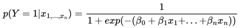
Below you can see the parameters of a logistic regression model and their graphical representation:
- Beta parameter: Also known as the coefficient, this parameter is estimated using maximum likelihood estimation (MLE). This is represented by β1, βn.
- Log likelihood function: This function is the logarithm of the likelihood function and is maximized to find the best parameter estimate.
- Intercept term: This is represented by β0.
Figure 14.
Logistic Regression Curve by Mendling et al. (2012).
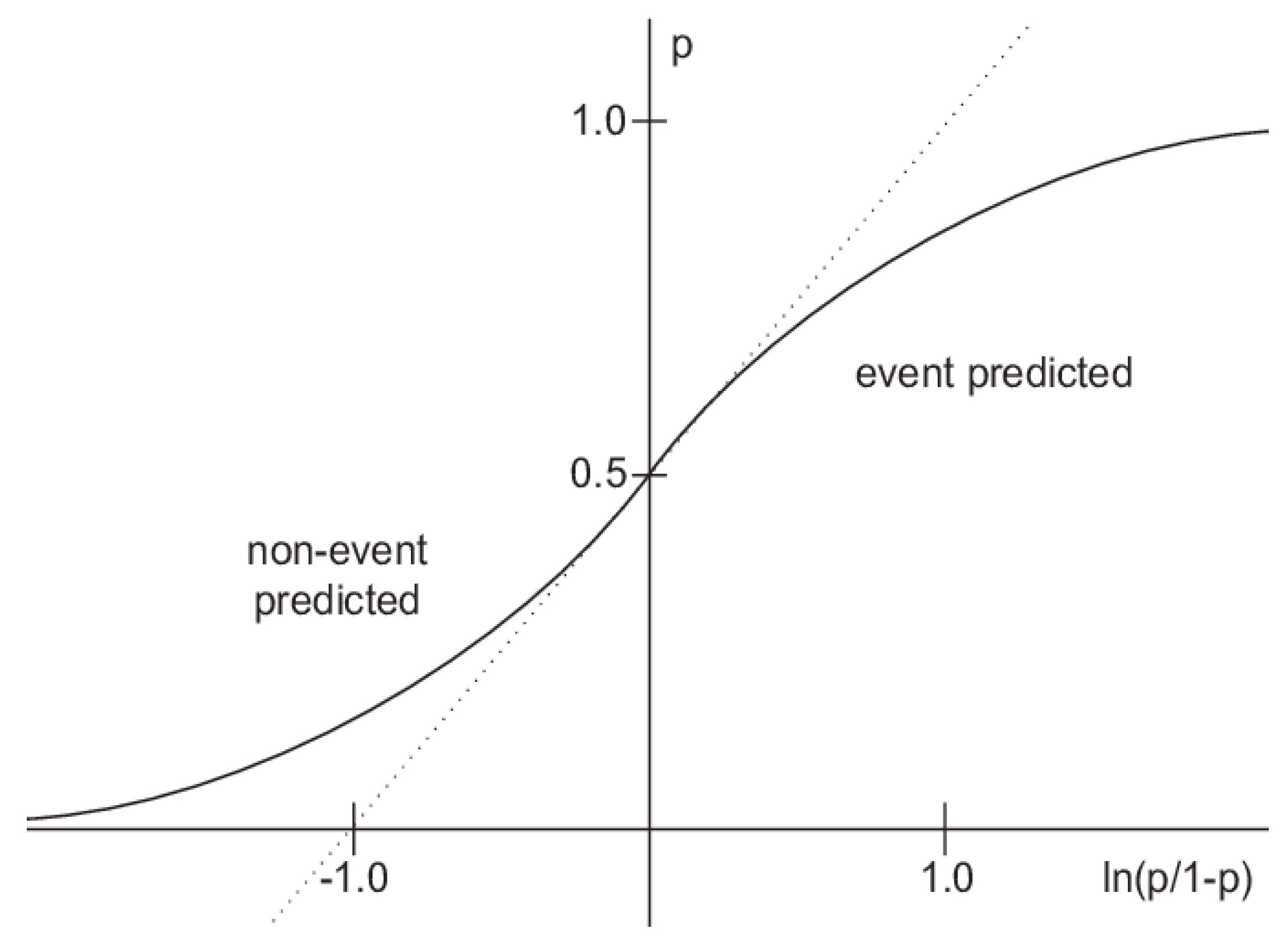
The use of logistic regression was certainly one of the main ways that Sumpter (2020) and his two students Marius Norheim and Jan Runo made consistent profits from sports betting in 2018. As a result, according to various public sources, they obtained a financial return of more than one million dollars.
Other notable examples of successful bettors include Tony Bloom, who is known for having amassed enough wealth to acquire Premier League soccer club Brighton, and Matthew Benham, who, according to Andrada (2021), has acquired another traditional Premier League club, Brentford, in the same way over the years.
Both of these clubs are also often used as case studies of soccer teams that use mathematical and statistical knowledge as a powerful weapon throughout competitions and have achieved impressive results in terms of cost versus benefit, from the administrative structure to the formation of the squad of players.
2.11.2. Horse Racing
In the 1980s, William Benter (2008) was one of several academics who raised the question of whether it was possible to beat the house using completely mechanized systems. In his particular case, he took his knowledge to apply to horse racing. It is known that Benter worked for basically a decade to develop a robust mathematical and computational model in order to obtain significant results in terms of profits from horse betting.
According to Silverman (2012) Benter, through his seminal study for the field of horse racing studies, employed and helped popularize advanced statistical models such as Conditional Logistic Regression, which has been extended over the years to include the Lasso technique, cyclic coordinate descent, among others for betting in this sense.
Just as Kelly Jr. (1956) suggested that it is only viable to enter a game when the mathematical expectation is positive for the player, Benter also focused on extracting value from sports betting, so that, through an extensive database containing, for example, variables such as the age of the horses, previous performances, the jockey in question, weather conditions, for
example, the bettor could identify entry opportunities and always have an advantage over the odds offered by the bookmaker. Through these small profit margins (as presented by Benter, between .25% and .50%) on each individual bet, over the long run, he was able to make a satisfactory profit.
It is common knowledge that Benter's adventures in betting, sometimes in company with his gambling partner Alan Woods, led to a profit of US$1 billion from betting and horse racing prediction software.
2.11.3. Dixon-Coles and the xG Expected Goals Model
According to Michels et al. (2023), it was through Maher (1982) that the academic community had its first systematic study on the analysis of goals from a probabilistic point of view, as well as the analysis of the “attacking strength” and “defending strength” of teams in men's soccer. In this study by Maher (1982), the Poisson model found it difficult to “match” the results of the games and so the author opted to continue his studies using the negative binomial distribution.
The Dixon-Coles model, introduced by Stuart Dixon and Stuart Coles (1997), according to Koopman and Lit (2015) is an extension of the Poisson model with a non-stochastic time function. As we can see from Sumpter (2017), the model evaluates the joint probability of the number of goals scored by two teams in a match, taking into account factors such as the strength of each team's attack and defense, as well as in a general context evaluating each team with the overall average of all teams in a tournament, as well as evaluating home-field advantages.
According to Altmann (2004) the basic modelling of this model assumes that the number of goals X and Y, scored by the home and away teams respectively, follow independent Poisson distributions:
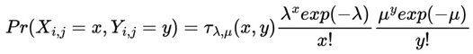
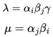
The Dixon-Coles model adjusts this structure, introducing dependencies in cases of low goal count (e.g., 0-0 or 1-1), through an adjustment factor (ρ), which corrects the overestimation or underestimation of probabilities. The Dixon-Coles model is a very useful methodology for analyzing team performance over time and, to a certain extent, serving as a way of “predicting” future results.
In addition to the Dixon-Coles model, as pointed out by Sumpter (2017) the xG (expected goals) metric is a more recent approach, developed with the aim of quantifying the quality of shots in soccer. Each goal attempt is assigned a probability of success between 0 and 1, based on contextual characteristics such as the distance and angle of the shot in relation to the goal; part of the body used (feet, head, etc.); position and movement of players and opponents, dividing the field into “zones” and thus calculating the respective probabilities as pointed out by Rathke (2017), analysis of goal opportunities through set pieces according to Spearman's OBSO model (2018), among other possibilities.
Figure 15.
xG Model by Hewitt e Karakuş (2023).
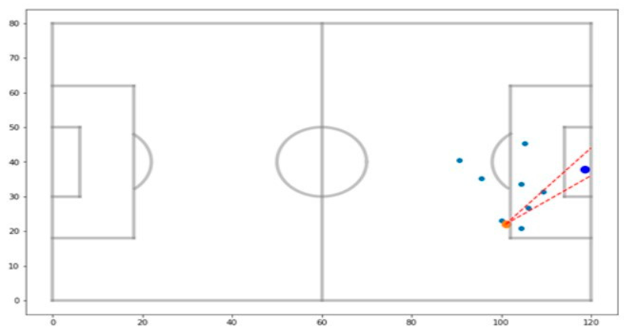
Normally, to determine the value of xG for a specific shot, we can use non-linear regression, logistic regression, as well as machine learning algorithms, as presented by Hewitt and Karakuş (2023).
According to studies carried out by Umami et al. (2021) after analyzing the results of all the events of the 5 main soccer leagues in Europe in the 2019/2020 season, we can reach some conclusions such as:
- Most kicks occur between 10 and 20 meters away,
- Kicks with distances equal to or less than 6 meters or kicks with distances equal to or greater than 34 meters, are considered to occur very infrequently,
- As expected, players rarely take kicks from less than 5 degrees, corresponding to a center shot close to the goal.
The xG model, unlike the Dixon-Coles model, aims to evaluate more specific contexts within a soccer match, for example, when evaluating the teams' performance in terms of quality, such as analyzing the ratio between the number of goals scored and the number of chances created by the teams given certain parts of the pitch. In this sense, for example, a frontal shot 15 meters from the goal may have an xG of .325 (32.5%) probability of being converted. It is also used to quantify the impact of teams' tactical decisions. Another notable study, we can see that Hirotsu and Wright (2002) adopted the Markov process model to analyze the optimal time period for substituting players as well as making tactical decisions on the pitch in a soccer match.
As highlighted by Yates (2023), the deliberate search to predict future results is a natural part of being human; however, according to Spiegelhalter et al. (2011) we must be careful not to fall into mental traps that can cause us to see patterns where none exist. In this sense, it is important that when we try to model phenomena in which the uncertainty factor is very present, as is the case with sports, the scientific method, mathematics and statistics will be our main allies in identifying coherent patterns.
2.11.4. Artificial Intelligence Applied to Sports Gambling
In times when technologies such as Artificial Intelligence and its offshoots like Machine Learning and Deep Learning are becoming increasingly popular, it is worth considering that they could also be allies for users in the art of making predictions.
Among some studies we can highlight Hubáček et al. (2019) who used machine learning models that demonstrated it is possible to obtain cumulative profits in basketball games with the NBA case study; Friligkos et al. (2023) applied the logistic regression model combined with Artificial Intelligence as a means of predictive analysis in tennis games and; Kim (2023) demonstrated that his CNN (Convolutional Neural Network) algorithm was useful for predicting 494 out of 540 possible outcomes of Korean professional basketball matches after considering more than 70 variables in his model, as well as analyzing wins with 5 or 6 point advantages, for example, during the 2017/2018 to 2022/2023 seasons.
2.11.5. Moneyball
Lewis (2004) goes into great detail about the story of triumph starring Billy Beane - a general manager of the Oakland A's - a traditional baseball team who, experiencing chaos in his team, such as sudden budget cuts and internal problems, begins to look for ways to develop a competitive team with the smallest possible budget.
It is known that Beane meets up with the young and brilliant Paul DePodesta, who becomes his assistant. During this time, they began to apply advanced statistical and analytical models to the world of sports. As discussed by Lewis (2004), statistical models indicated the signing of players, generally of dubious ability (according to what baseball experts knew at the time), who could be very important if placed in suitable positions by evaluating aspects such as batting average and player speed.
Taking into account the potential of these statistics and data science tools, the Oakland A's had become one of the greatest teams in baseball history in the 2002 Major League Baseball (MLB) season by winning 20 consecutive games and, shortly afterwards, the team won the American League West Division. Despite not succeeding in the post-season, in which they were eliminated, the story of the Oakland A's has become one of the most emblematic examples to be followed, as they have shown that it is possible to obtain excellent results even with few resources using science and statistics and their techniques.
2.11.6. Arbitrage (Surebet)
According to Buchdahl (2003) arbitrage (also known as surebet) in sports betting is a strategy based on exploiting discrepancies between the odds offered by different bookmakers for the same sporting event. This phenomenon occurs due to differences in probabilistic modeling, manual adjustments in the markets and variations in betting demand. The principle behind sports arbitrage is similar to financial arbitrage, where an asset is traded simultaneously on different markets to make a risk-free profit. Buckle and Huang (2018) demonstrated the study and practical applications of arbitrage in rugby matches.
Mathematically, arbitrage occurs when the sum of the implicit odds of an exhaustive set of bets is less than 1. Formally, let O1, O2,..., On be the odds offered for the possible outcomes R1, R2, ..., Rn of an event. We define the implicit probability of each odd as:

If the sum of these probabilities is less than 1:

Consider a tennis match between two players, A and B, and two different bookmakers, each offering odds for both players to win:
Table 5.
Arbitrage analysis in a hypothetical tennis match.
| Bookmaker | Odd for A to Win | Odd for B to Win |
|---|---|---|
| Bookmaker 1 | 2.1 | 1.8 |
| Bookmaker 2 | 1.95 | 2.05 |
To identify an arbitrage opportunity, we check the implied probabilities of the best odds available from the various bookmakers analyzed:
Best odd for A to win: OA = 2.10 (Bookmaker 1)
Best odd for B to win: OB = 2.05 (Bookmaker 2)
We calculate the implicit probabilities:
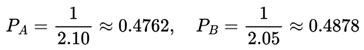
adding up the probabilities,

As 0.964 < 1, there is an arbitrage opportunity.
Now, as another hypothetical example, let us calculate the optimal allocation for a total bankroll of €100. The fraction of the capital to be bet on each outcome is given by:
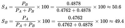
If we bet €50.6 on A to win and €49.4 on B to win, the return will be:
- If A wins: 50.6 × 2.10 = €106.26
- If B wins: 49.4 × 2.05 = €101.27.
The net profit for team A if they win will be €6.26, which means a return on investment of 6.26%. On the other hand, if team B wins the net profit will be €1.27, meaning a return on investment of 1.27%. In both scenarios we see a guaranteed profit for the bettor, regardless of the outcome. As we can see, in addition to positive mathematical expectation, bettors have the arbitrage technique as a tool that mathematically offers risk-free bets.
Grant et al. (2018) analyzed arbitrage opportunities in the soccer betting market, showing that bookmakers' management practices, such as limiting amounts to be bet and even excluding accounts, limit their exploitation by bettors. The authors classified bookmakers into two large groups: position-takers, who adjust odds infrequently but impose restrictions on informed punters, and book-balancers, who adjust odds constantly but apply fewer restrictions on punters. According to the results, 545 arbitrage opportunities were identified, but around 50% involved betting on the favorite with position-takers, whose operational restrictions make arbitrage unfeasible in practice.
We can say that the bookmakers' management practices, as well as possible miscalculations on the part of the bettor and, generally, a short period of time to analyze different odds at various bookmakers, make this one of the main limitations of this technique in the world of sports betting.
2.11.7. To Win, To Lose, To Fail to Win, To Avoid Losing and To Break Even
We can say that within the world of sports betting, there are 5 fundamental elements to understand and which are crucial and constantly present in the life of any bettor. These include:
Table 6.
Some of the elements that make up an understanding of the world of sports betting.
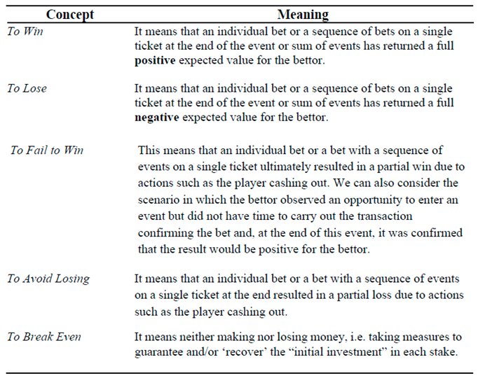
In addition to the mathematical and statistical approach, although it is not clearly well documented in academic materials, understanding these 5 elements mentioned above can be crucial for a bettor to be characterized as “professional” or not, i.e. one who bets only occasionally for “fun”. As we can also see, these 5 elements are more directly linked to the emotional aspect of the person.
In the world of sports betting there is a consensus that there is only a small proportion of bettors, usually between 2% and 5%, who are constantly profitable and, therefore, another proportion of these, with betting being a significant part of their sources of income. Therefore, we can infer it is a market in which the vast majority of bettors will have a negative expected value in the long term, mainly due to some factors such as the absence of:
- bankroll management;
- knowledge in statistics and mathematics;
- knowledge of the sport in question;
- understanding the world of sports betting;
- emotional aspects.
As we can see above, there are a number of factors that make the vast majority of bettors unprofitable in the long term, in addition to the fact that mathematical expectation is naturally against the bettor due to administrative fees. Among these factors, surely the most important is the emotional factor, from advertising issues as a way of making money in a short space of time in front of their electronic devices to the randomness factor present in sporting events.
Another important point is that bettors don't reconcile their realistic winning expectations with the value of their stake and the size of their bankroll. It is too complicated to stipulate what would be a certain range of values in which we can consider a “realistic expectation” of daily winnings due to its subjective nature. However, one pattern I have observed over the last few years is that among those sports traders who consider themselves ‘professionals’ and make a living from it, the 'realistic expectation' of daily winnings usually ranges from 0.25% to 2% of the total value of the bankroll per day.
Therefore, those who don't have a basic financial education may be susceptible to exposing themselves to more unnecessary risks and, as a result, wearing themselves out more. When it comes to bankroll management aligned with emotional management, there are two classic mistakes which are responsible for many bettors losing money. We can mention the practice of “all win”, i.e. putting all the money in the bankroll on a single bet and deliberately trying to recover as quickly as possible any amount lost on previous bets, which further increases the financial losses for the bettor.
Another important point to highlight, the number of bets does not necessarily imply greater winnings and ‘money’ for the bettor. This is another classic mistake which, in addition to exposing oneself to a greater tendency to financial losses, also corroborates the possibility of increasing the tendency to become a betting addict.
Inevitably, I was able to observe another pattern: professional bettors usually spend a good part of their lives living in a dice paradise, i.e. betting is basically their profession, and they have more time to analyze data and statistics about the sport in question. What's more, they tend to have an income that allows them to “train” their betting strategies as well as a mind trained to deal with the psychological biases that are natural in this environment.
What I mean is that, considering that a large part of a nation's population is considered to be struggling for basic survival and adding advertising issues, psychological biases, the randomness factor of sports and the lack of basic knowledge of finance, mathematics and statistics, this population tends to be more vulnerable and, therefore, this can explain why the vast majority of bettors tend to lose money in this market. We are starting from a principle similar to that addressed by Kahneman and Tversky (1979) that the impact of a financial loss resulting from a sports bet tends to have an even more significant impact on this sub-group of the population, since, when fighting for basic survival, every loss tends to be felt even more, which can get out of hand with the emotional side of these people.
Still on emotional aspects, Walker et al. (2008) highlight the contradiction between the economic logic of “expecting to win” and the behavior of the modern gambler, i.e. playing even with the expectation of losing, and propose that psychology needs to explore more deeply the motivations behind this activity.
It is common to observe that some government institutions place all the blame for this scenario on sportsbooks and advertising media as a way of mitigating the level of their incompetence in managing the public good, which we can see as somewhat misguided. However, if these same people could have a decent life expectancy and a decent job opportunities, those who enter this world of sports betting precisely for financial reasons would probably rethink things several times over without having any prior knowledge of basic fundamentals. Therefore, there is a whole economic, political and social context behind the boom in sports betting and its consequences around the world.
Even if a person has all the financial peace of mind, time and robust knowledge of the mathematics behind this market, there are still cognitive factors and the inherent randomness of the game that can affect them in some way, after all, we are all human beings and we are not immune to mistakes and bad luck. It is a challenging market, but it is possible to beat it in practice, consistently over the long term.
In short, the world of sports betting goes beyond the mathematical and statistical aspects to include other areas such as knowledge of the sport itself, as well as psychology and randomness in the sense of unexpected events. Next, we'll look at the ‘equation’ that shapes sports betting from a bettor's point of view:
Bettor's equation = Knowledge of the sport + Knowledge of finance, mathematics and statistics + Psychological factors + Random noise.
2.12. Psychological and Statistical Bias
2.12.1. Humaness vs Randomness
Human beings are naturally terrible at trying to generate a sequence of numbers that they consider random. Although this discussion is not new and has been documented by Teigen (1983) we see that, for example, when we put several people from different parts of the world to choose from a range of 1 to 12, the number that stood out the most was the choice of number 7. This may be due, among other reasons, to the fact that people, in an attempt to appear random, end up disregarding the choice of numbers at either end of the range.
Other experiments over this time have also been carried out by fellow scientists and, even if we consider a wider range of numbers, for example between 1 and 50, the number 7 or some other “central” numbers such as 27 are also chosen more often than the others. It is certainly a very interesting exercise to do in order to verify in practice this human bias that seems to be timeless.
One of the most recent studies in this line of research is Van Koevering and Kleinberg (2024), whose aim was to assess the level of humaness when faced with the process of generating random sequences. This paper provides us with an interesting discussion about the natural inability of human beings to try to be "random". Therefore, when placed in an LLM (Large Language Model) approach, we will see that when machines have a randomness bias in their database due to the human factor, they also tend to reproduce these biases. In some cases, much worse than the sequences generated by humans.
2.12.2. Controversies of the Sports Betting World
Contrary to the colorful world of the small percentage of constantly profitable users, there is a rather dark side to the majority of users. Although the business model of bookmakers is to offer their users an entertainment, we can't ignore the fact that with the impression that they can obtain a quick financial return easily accessible from a mobile device or computer, many users in turn end up “naturally” considerably increasing the risk of becoming addicted to betting.
Yüce et al. (2022) carried out a robust study on the possible main motivations that lead an individual to become addicted to gambling. Among their main findings were that individuals who enter a bookmaker with the intention of making money, socializing or simply being in a game in the sense of getting something in return, are certainly much more likely to become addicted. On the other hand, those individuals who are aware that this business should only be seen as a sporadic source of entertainment, fun and just getting to know how a sport or bookmaker works, will be less likely to become addicted to gambling.
According to Killick and Griffiths (2021) through their extensive systematic review of 22 papers on the subject, they came to the conclusion that the most significant impact of sports betting marketing is observed in individuals who already show signs of gambling problems.
This suggests that marketing can exacerbate existing gambling problems. As such, it is a further means of drawing the attention of public authorities to the health and economic impacts.
The impact of this world of betting is already having a strong influence on the economies of nations around the world. In Brazil, for example, according to a report by XP Investimentos (2024), this market has an average annual turnover of approximately 22 billion US dollars. In this sense, supermarkets, for example, have seen a decrease in consumption, since this percentage, which could be used to boost this and the most diverse sectors of the economy, is being used exclusively for sports betting. Thus, we can say that betting has been a strong “competitor” for other sectors of the economy and, therefore, has increasingly become part of the culture of a people in different nations.
Heine (2022) has pointed out that online sports bettors tend to be younger and spend more money than other types of gamblers. This concern for young people was also well addressed by Aragay et al. (2021). In addition, online gambling is becoming increasingly normalized and easily accessible. The "faceless" nature of online platforms removes some of the barriers associated with traditional gambling, making it easier for anyone to participate. In Brazil, for example, it has been observed that pensioners as well as people who receive some kind of government aid because they are in situations of social vulnerability have also used part of their savings for sports betting.
Another relevant point highlighted by Heine (2022) was the correlation between gamblers, especially young gamblers, acquiring other addictions, such as alcohol and other drugs, as well as acquiring depression later in life. This suggests a possible link between gambling and other risky behaviors, which is important to consider when thinking about long- term consequences.
2.12.3. Why Do Some Bettors Lose More Money Than Others in Sports Betting?
The study by Buhagiar et al. (2018) investigates why some soccer bettors lose more money than others by analyzing the presence of the favourite-longshot bias. In efficient betting markets, bettors are expected, on average, to break even before costs but consistently lose after costs due to the bookmaker's margin.
The authors applied a sample of 163,992 odds from ten European leagues, and tested some hypotheses about whether the excessive losses of some bettors stem from behavioral bias or the inherent unpredictability of certain sporting events. As a result, this study confirms the favourite-longshot bias in soccer, but reveals a finding that was not initially anticipated: bookmakers' odds are better predictors for underdogs than for favorites when considering the Brier score. This suggests that bettors preference for underdogs can amplify their losses, not only because of the adverse odds, but also because bookmakers model these events better than the bettors themselves.
Buhagiar et al. (2018) also emphasized that the greater the accuracy of bookmakers in predicting sports results using their robust databases and machine learning techniques, the greater their profits will be and, consequently, the greater the losses for bettors in the long run due, above all, to the law of large numbers and the bookmaker's fee itself embedded in the calculation. In this sense, the authors also raised the importance of policy-makers re-evaluating the issue according to the traditional economic model that new competitors in this sports betting market will not cause bettors to lose less money, but quite the opposite.
2.12.4. Ostrich Effect
The “Ostrich Effect”, a term coined by Galai and Sade (2006), is a psychological bias in which the individual avoids negative or threatening information, even if it is relevant to decision- making. The term derives from the popular belief that the ostrich, when it feels threatened, sticks its head in the sand, ignoring the danger. In real life, an individual may seek to protect themselves from negative emotions, such as fear, anxiety or stress, by avoiding information that could trigger them.
As predicted by the ostrich effect, Galai and Sade (2006) in their seminal study of financial market investors found evidence that the difference in return between liquid assets (T- bills) and illiquid assets (bank deposits) is greater in periods of greater uncertainty. This suggests that investors prefer to avoid the discomfort of facing negative information in times of uncertainty by opting for illiquid assets that provide fewer market updates. As we saw earlier, although the preference for illiquid assets in times of uncertainty can be influenced by multiple factors such as the search for security and risk aversion under uncertainty, it is notable that the ostrich effect played a relevant role in the results.
According to Karlsson et al. (2009) through their innovative approach in their decision- theoretic model on selective attention to information, ostrich-like behavior transcends the field of finance and can be present in various areas of life since the avoidance of something can manifest itself in various ways, such as ignoring negative news, avoiding conversations on unpleasant topics or procrastinating important tasks. Parents who take their children to the doctor's office for tests for some kind of illness or disorder and people who are about to undergo tests to check if they have contracted a sexually transmitted disease can exhibit this same behavior. It is therefore an important concept in the field of behavioral economics, which also shapes the global economy.
2.12.5. Kahneman and Tversky Approaches
Over several decades Kahneman and Tversky have carried out several seminal studies in the field of psychology and behavioral economics which have led to the development of many important concepts for this field of study, some of which are directly related to the world of sports betting.
Tversky and Kahneman (1974) came up with the concept of the Anchoring Effect, which is a psychological bias in which individuals have a tendency to rely too much on an initial piece of information (the “anchor”) when making decisions. In sports betting, the anchor can be an initial tip, a statistic or an expert comment, even if this information is not entirely reliable.
Bettors can use these anchors as a reference for their own decisions, which can lead to distorted assessments of the odds and inappropriate betting choices based on subjectivism and emotions rather than rational, probabilistic thinking.
In their seminal paper, Kahneman and Tversky (1979) introduced Prospect Theory, which describes how people make decisions under risk and uncertainty, challenging the widely accepted Expected Utility Theory of classical economics. Prospect Theory shows that people don't evaluate gains and losses in a linear way, and exhibit loss aversion, i.e. losses are weighted more heavily than gains. In addition, another important concept raised was reference dependence, i.e. choices are influenced by a perceived reference point.
Among the key components of Prospect Theory are functions such as concavity for gains, that is, people are generally risk-averse when it comes to gains. As an example, the difference between a gain of $100 and $200 feels greater than the difference between $900 and $1000, even though the absolute difference is the same. Another important function we have convexity for Losses, that is, people are generally risk-seeking when it comes to losses. The pain of losing
$100 is felt more strongly than the pleasure of gaining $100. This can lead to people taking greater risks to avoid a sure loss.As a consequence, losses are perceived as steeper than gains, that is, loss aversion means that the pain of a loss is felt more strongly than the pleasure of an equivalent gain. This is often expressed as a ratio—for instance, losing $100 feels about twice as bad as gaining $100 feels good, for example, a loss of $100 feels about twice as bad as a gain of
$100 feels good. These examples can be better explored by looking at the image below.
Figure 16.
A Hypothetical Value Function by Kahneman and Tversky (1979).
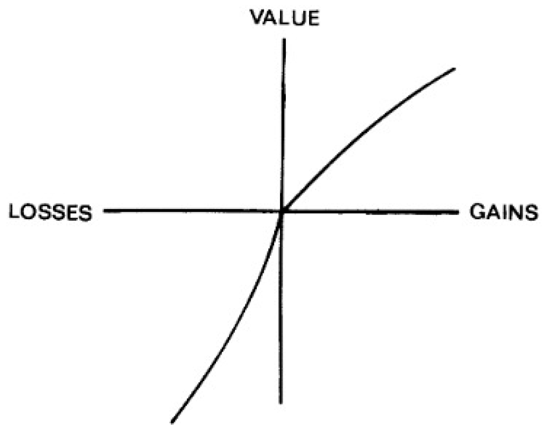
Kahneman and Tversky (1979) also raised the so-called Weighting Function, which describes how individuals perceive probabilities. It suggests that:
- Small Probabilities are Overweighted: people tend to overestimate the likelihood of rare events, especially when those events are highly salient, e.g., winning the lottery, being involved in a plane crash;
- Moderate and Large Probabilities are Underweighted: people tend to underestimate the likelihood of common events;
- Certainty Effect: people place a disproportionately high value on outcomes that are certain, compared to outcomes that are merely probable, even if the difference in probability is small. This drives risk aversion for gains and risk-seeking for losses near certainty.
Prospect theory has had a profound impact on various fields, from finance, marketing, negotiation to public policy. As for the field of study of the sports betting world, we could say that Prospect Theory through the concept of loss aversion can mean that a bettor who has already suffered significant losses may feel inclined to place riskier bets, with very high odds, in the hope of recovering everything at once, distorting the real probabilities of success and further compromising their bankroll management.
2.12.6. Momentum Effect on Sports Betting
Moskowitz (2021) deepened his studies on the world of sports betting from the perspective of risk analysis and bettor behavior by testing whether betting returns are explained by behavioral theories (investor bias) or rational asset pricing models.
The author demonstrated after analyzing 100,000 contracts over three decades that in sports betting there is no systematic risk as there is in other financial markets, but rather “momentum” and exogenous terminal values, i.e. the results of matches. In this sense, momentum can be described as the behavior of bettors to give more “value” to the recent behavior of favorite teams that have performed excellently in recent matches.
This lack of analysis of a team's long-term performance over a longer period of time tends to lead bettors/investors to over-react (rather than rationally pricing). The effect is similar to what happens in the financial markets, where stocks that have performed well recently tend to attract more investors, generating a price bubble. As a consequence, these bettors face much greater risks due to this natural imbalance of odds due to the psychological biases that resonate with most bettors, influencing the market as a whole. It is known that after the moment of euphoria, prices tend to adjust to the natural pattern.
With the momentum effect as a basis, Moskowitz (2021) analyzed contract opportunities by betting against the momentum effect. As a result, the strategy of betting against momentum could generate an average return of 6.34% per year. An interesting return in which we could place it in the category of beating the house, however, due to the existence of bookmaker fees this option becomes mostly not applicable and/or not 'rewarding' for the bettor in the long term. Vizard (2023) also analyzed the momentum effect in his study and reached similar results in line with the theory of limits to arbitrage, which suggests that certain inefficiencies in this market may persist because costs and restrictions prevent traders from fully exploiting them.
2.12.7. Gambler's Fallacy
According to Clotfelter and Cook (1993) in their studies on the behavior of gamblers in lottery games, the gambler's fallacy, also known as the Monte Carlo fallacy, refers to the erroneous belief that the ocurrence of a random event influences the probability of subsequent independent events. This psychological bias is predicated on the misconception that deviations from expected statistical distributions must be corrected in the short term, leading individuals to anticipate a reversal of outcomes following a sequence of similar events.
Formally, the gambler’s fallacy can be illustrated within the context of a sequence of Bernoulli trials, where each trial is statistically independent and identically distributed. Consider a ‘fair coin’, where the probability of heads or tails is uniformly P(H) = P(T) = 0.5 for each trial. The fallacy manifests when an observer, after witnessing a series of heads, irrationally concludes that the probability of tails in the subsequent trial is elevated, disregarding the independence of each event.
Despite different approaches, Taleb (2016) explores psychological biases, above all by describing the role of randomness and chance in our lives, especially in the financial markets. Taleb argues that we often confuse luck with skill and fail to recognize the impact of uncertainty, the natural random noise present in outcomes.
Another point to highlight in Taleb's (2016) work is the survivorship bias, i.e. people tend to want to hear about those who have succeeded (survivors), ignoring the vast majority who have failed, which leads us to overestimate the effectiveness of certain strategies.
2.12.8. The St. Petersburg Paradox
The St. Petersburg Paradox is a classic problem in decision theory and mathematical economics, introduced by Daniel Bernoulli (1738). It illustrates a scenario in which the mathematical expectation of a gambling game is infinite, but, paradoxically, most people would not be willing to pay a high amount to participate.
The game consists of a fair coin that is tossed repeatedly until the first “face” occurs. The prize paid to the player is 2n monetary units, where n is the number of tosses needed to get the first “face”. Thus, the payout is structured as follows:

The expected prize value is calculated as:
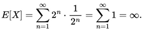
This at first suggests that a rational agent should be willing to pay any amount to take part in the game, since its expected value is infinite. However, empirically, individuals do not demonstrate this willingness, which sets up the paradox.
Bernoulli argues that individuals don't make financial decisions based solely on the mathematical expectation of return, but rather on the expectation of expected utility. This principle is one of the explanations why people would not be willing to pay large sums to enter the St. Petersburg game, even though its expected value is infinite
He also suggested that individuals evaluate monetary gains by means of a concave utility function, such as logarithmic utility:
which leads to a finite expected value for the game and justifies why agents wouldn't pay arbitrarily high amounts to participate. Below is a figure illustrating Bernoulli's theorizing.
U(x) = ln(x),
The Figure 17 of Bernoulli's utility curve (1738) visually represents the idea that a person's satisfaction with wealth increases at a decreasing rate. This idea is fundamental to the author's solution to the St. Petersburg Paradox, as it explains why people don't act according to the infinite expected value of the game, but rather the expected utility, which is not infinite due to the diminishing marginal utility of money.
Figure 17.
Bernoulli's Utility Curve (1738).
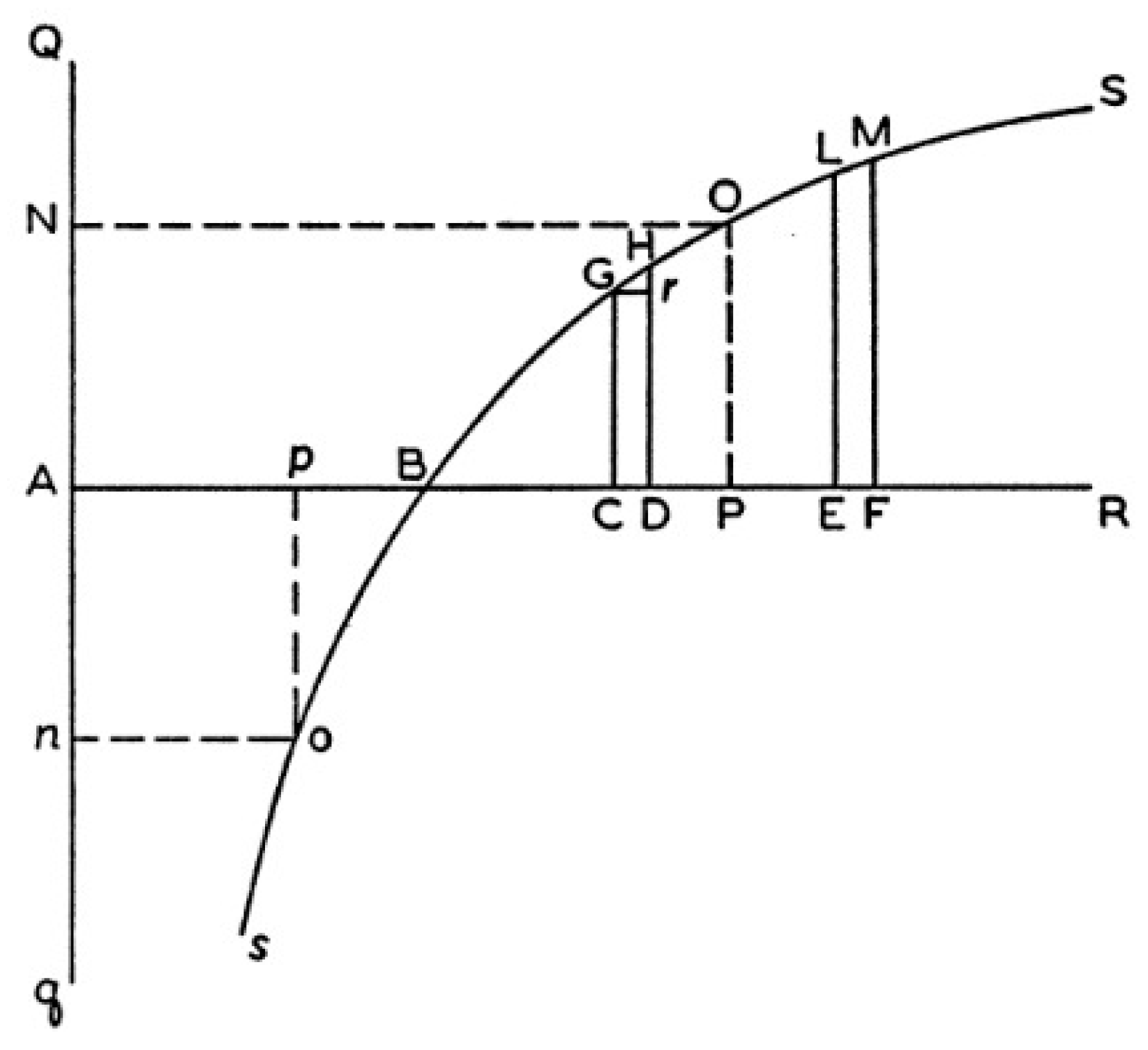
2.12.9. Simpson’s Paradox
As Bonovas and Piovani (2023) pointed out, the expression paradox comes from the Greek word paradoxon. In this sense, it refers to everything that contradicts common sense, thus making a strong intersection between logic and philosophy.
Simpson's paradox is a statistical phenomenon in which a trend observed in several separate groups is reversed or disappears when these groups are combined. This paradox arises when the analysis of the sum of all the data leads to a different conclusion from the analysis of the separate data, due to the presence of hidden variables (or confounding variables) that affect the results. This illustrates how, in certain situations, the interpretation of data can be misleading if we don't consider the relevant subdivisions or variables, which can consequently lead us to make the wrong decisions.
Figure 18.
Simpson’s paradox or the Yule–Simpson effect. A correlation between gene A expression and gene B expression appears to be positive when cells are thought to belong to different cell types (blue and red) and negative when cells are thought to represent one cell type (black, dashed). Golov et al. (2016).
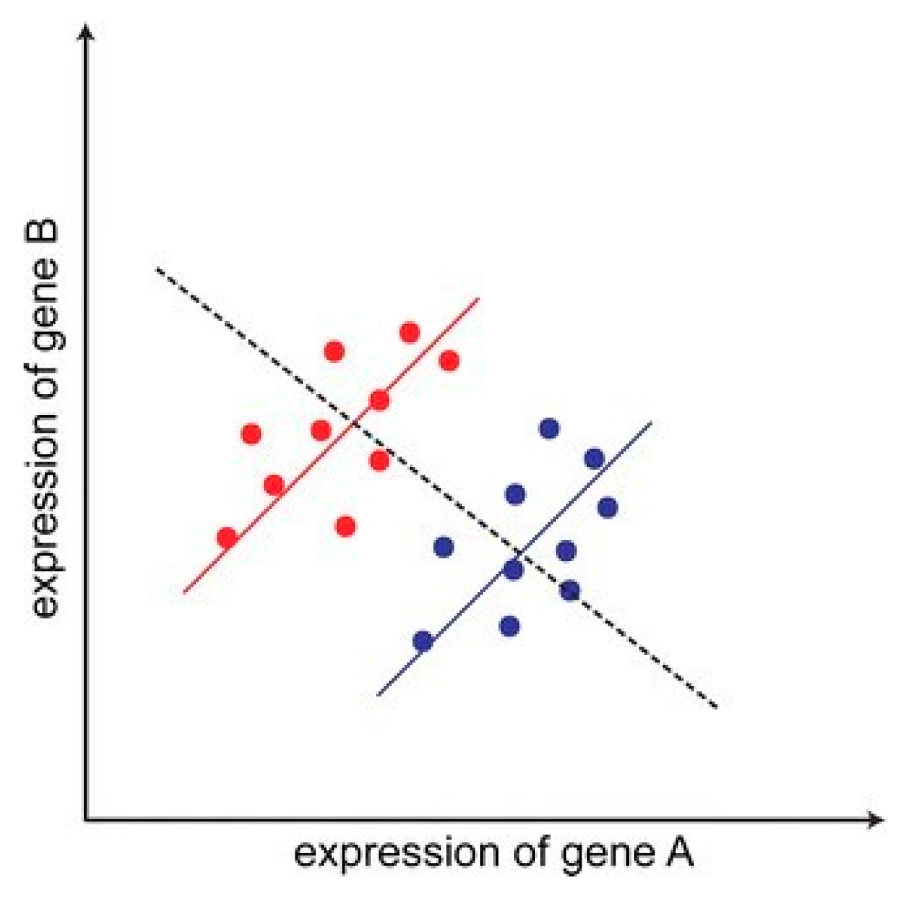
Although this paradox was first published in a technical paper by Simpson (1951) and, a few years later through Blyth (1972) was finally coined “Simpson's Paradox”, we see that other scientists in earlier periods came to similar conclusions in their studies, as was the case with Karl Pearson (1899) and Yule (1903).
Simpson's Paradox is very important for studies in various fields of science, however, it has been best known and constantly used in areas related to biological sciences through biostatistics. Some examples of its application in the field of biostatistics include the results published by Kügelgen et al. (2021) to analyze the dynamics of the COVID-19 pandemic by separating age-related effects from other unrelated variables and, more recently, the work of Bonovas and Piovani (2023) to analyze this paradox in clinical research.
2.12.10. The Berkson’s Paradox
The Berkson's paradox, also known as selection bias or Berkson's fallacy, describes a situation where statistical dependence between two attributes that are marginally independent in the general population appears as a negative correlation when observed within a restricted sample. This phenomenon arises when the sampling process is conditioned on the presence of at least one of the attributes, leading to a skewed representation of the population. Consequently, the observed association within the sample can lead to erroneous conclusions about the relationship between the attributes in the broader population from which the sample was drawn.
Belair (2025) shows us a classic example of this paradox in medical studies. Suppose that two diseases are independent in the general population, but the sample is taken only in one hospital. If the patients in the hospital tend to have at least one of the diseases, it may appear that the two diseases are negatively correlated, which is an illusion caused by selection bias.
Although both Simpson's Paradox and Berkson's Paradox are formally statistical biases, we can say that, in parts, they are also psychological biases, since our minds tend to simplify or generalize patterns without considering nuances or deeper contexts.
This paradox underscores the critical importance of considering sampling mechanisms when interpreting statistical associations, particularly in contexts where data collection is non- random and conditioned on specific characteristics.
2.13. Game Theory
2.13.1. A Brief Historical Context of Game Theory
According to Packel (2006) a game can be understood as a set of players who follow a set of established rules in which their actions and strategies lead them to different end results containing n payoff values. In this sense, the game theory is a branch of applied mathematics dedicated to the study of strategic situations in which individuals or entities (called “players”) make decisions that mutually affect their outcomes. In other words, game theory seeks to model and analyze situations of strategic interaction, where one player's choices directly influence the rewards or penalties of other players.
As Osborne (2004) pointed out, Game Theory is a vast field that goes beyond the boundaries of games, serving to understand and model economic, political and biological phenomena, for example. As with other sciences, according to Barron (2024) Game Theory is built and sustained through models, which are based on our abstractions that occur through our observations and experiences of the natural world.
Although game theory is a relatively recent field of science, according to Bortolossi et al. (2017) it had already been developed little by little by some scientists around the world when dealing with certain concepts are predominant today.
According to Bellhouse (2007) and Bortolossi et al. (2017) in 1713, the concept of Mixed Strategy emerged through the game Le Her, a study carried out by James Waldegrave (1684- 1741) and described by him in a letter to Pierre Rémond de Montmort (1678-1719) who in turn met a short time later with Nicholas Bernoulli to discuss the work and the publication of the work “Essay d'analyse sur les jeux de hazard” took place. This study sought to demonstrate a strategy that maximized the probability of success regardless of the opponent's choices. In this sense, it was a great reference for the emergence of new studies on mixed strategies over the years.
As highlighted by Bortolossi et al. (2017) more significant advances occurred from the 20th century onwards, when Ernst Zermelo (1871-1953), in 1913, published a theorem on the game of chess in an article entitled “Uber eine Anwendung der Mengenlehre auf die Theorie des Schachspiels”, stating that, in the course of a game, at least one of the players has a strategy that will lead to victory or a draw.
As pointed out by Osborne (2004), Game Theory gained further development from the 1920s onwards through the pioneering work of Emile Borel (1871-1956) who, as can be further explored in Bortolossi et al. (2017), published notes on symmetrical zero-sum games with two players and a finite number of pure strategies for each player, as well as pioneering approaches to the development of other important concepts such as pure strategy in which according to Chen (2022) a player chooses a single action with certainty and, mixed strategy, a player chooses randomly between several actions, with specific probabilities, for example.
According to Osborne (2004), game theory began to be highlighted as an individual field through the pioneering articles by von Neumann and Oskar Morgenstern (1944) in their work entitled “Game Theory and Economic Behavior”. Other important developments in this field as highlighted by Osborne (2004) were made by John Nash in the 1950s and, a little later, in the 1970s, with the emergence of game theory applied to the field of evolutionary biology, whose outstanding works we can mention Maynard Smith, a British theoretical biologist who applied the concepts of game theory to understand the evolution of animal behavior. His seminal works, such as “The Logic of Animal Conflict” (1973) and “Evolution and the Theory of Games” (1982), are considered fundamental milestones in the development of evolutionary game theory.
A notable paper was Stackelberg's (1934) approach which provides the academic community with a sequential game model in game theory, where one company - the leader - makes a decision first, and another company - the follower - observes this decision and then makes its own decision. This approach contrasts with the classic and important economic model of Cournot (1838) in oligopoly scenarios, where companies make decisions simultaneously.
Among some practical applications of Stackelberg's (1934) approach we can mention Kar et al. (2017) who applied this theoretical basis to analyze issues involving public and private security from security measures in ports through illegal practices to cyber attacks by modeling the relationship between attackers and attacked.
The authors Staňková et al. (2019) as well as Wölfl et al. (2022) analyzed that the interactions between doctors and cancer cells can be modeled through game theory in which the Nash Equilibrium and Stackelberg Equilibrium were analyzed as well as the differential equations present in the Lotka (1925) and Volterra (1926) mathematical model. As a result, it was realized that the Stackelberg approach in which the doctor assumes the role of “leader” and the cancer cells as “led” can provide ‘advantages’ for the doctor that can influence some advantage for the elimination of cancer in patients. Another important result was that the Lotka-Volterra (LV) model with its more specific approach to population dynamics supports strategies such as adaptive therapy, showing that controlling the evolution of the tumor can be more effective than aggressively trying to eradicate it.
Anscombe and Aumann (1963) published a seminal paper that provides a rigorous axiomatic basis for subjective probability. In essence, the authors sought to answer the question: how can we mathematically formalize the notion of probability when it represents an individual's personal beliefs, rather than objective frequencies? Although their implications are also concentrated on the field of Decision Theory, that is, according to Osorio (2010) on the aspect of analyzing better decision-making under uncertainty from the point of view of an individual rather than the dynamics of two or more players as occurs in game theory, we see that they have raised an important basis for dealing with and measuring uncertainty.
Harsanyi (1967), by transforming games with incomplete information into games with imperfect information, developed a way of analyzing games where the players do not have complete information about the other players, transforming them into games with imperfect information, where uncertainty is represented by a nature player.
We say that the “player nature” defined by Harsanyi (1967) randomly determines the types of players (for example, their preferences, private information or available strategies). The other players observe their own characteristics, but not those of the others, making the game one
of imperfect information. This concept was another major advance for game theory, and later Harsanyi (1968) influenced the development of the concept of Bayesian Equilibrium.
Aumann (1974) in another innovative study presented the concept of “Correlated Equilibrium” in which he generalized Nash equilibrium by allowing players to coordinate their strategies by means of a common, possibly correlated signal. In this context, a mediator suggests actions to the players, and equilibrium occurs when no player has an incentive to deviate from the suggestion, given the adherence of the others. This formulation expands the scope of game theory, incorporating situations in which shared information influences strategic decisions, resulting in outcomes that can be more efficient than those achieved by the Nash equilibrium.
In this timeline, we also note that auction theory was also of great relevance to the development of game theory. Milgrom and Weber (1982) provided the academic community with the development of modern auction theory that can be applied to a wide variety of real- world situations. The authors showed how different auction formats can affect the behavior of bidders and the final price of the item.
Through this paper by Milgrom and Weber (1982), many others have emerged along similar lines of research, such as Thaler (1988), who demonstrated that bidders in auctions often overestimate the value of the item they are buying and as a consequence this can lead to significant losses for the winners of the auction. Klemperer (1999), Booth et al. (2020) as well as Jia (2023) can provide more in-depth information on this subfield of game theory.
As highlighted by Aumann (2024), the field of game theory is evolutionary rather than revolutionary, which suggests a slow and constant process of development, with new ideas building on and expanding previous ones. This study on Victoria corroborates his argument.
In addition to these, there have been many other contributions that have contributed greatly to this field, however, in order not to escape the objective of this study, we can settle for just these examples. Due to its wide-ranging nature, according to Norozpour and Safaei (2020) the applications of game theory are vast in our daily lives, from assisting in orthopedic surgeries, as can be seen in the study by Brown et al. (2022), in project management by Narbaev et al. (2022), in electoral analysis by Amuji et al. (2024), in international relations by Sharifzadeh et al. (2022) and in deep learning applications with statistical mechanics by Bouchaffra et al. (2024), for example.
2.14. Main Dualities in Game Theory
In the field of Game Theory there are a number of dualities. In the following sub-topics, we will look at some of these main concepts.
2.14.1. Cooperative Games and Non-Cooperative Games
2.14.1.1. Cooperative games
As Nash (1953) pointed out, the name “Cooperative Games” comes from the fact that two or more players are able to discuss the situation and establish a plan together. Therefore, we can say that “Cooperative Games” are those in which players can communicate, form coalitions and make binding agreements in order to meet particular needs as well as achieve a common overall goal.
Cooperative Games, as pointed out by Osborne (2004), is a field of study in which we can better understand how coalitions are formed, how people/institutions negotiate and allocate resources and establish a strategy by common agreement. As such, it is highly relevant to studies in Political Science and Social Science, ranging from negotiation practices between individuals and companies to international conflicts involving nations.
According to El-Nasr et al. (2010) the studies by Rocha et al. (2008) observed cooperative game design patterns such as: complementarity; synergies between abilities; abilities that can only be used on another player; shared goals; synergies between goals; and special rules.
Among the main examples of co-operative games are the classic ‘Prisoner's Dilemma’ originated according to Guerra-Pujol (2013) by the Canadian mathematician Tucker (1950) and
the ‘Battle of the Sexes’ originally addressed by Luce and Raiffa (1957), which is a game that models the coordination of activities between two players with different preferences, for example.
Game Theory is very broad and, as a result, allows us to identify countless sub-variations of game types and even extensions of the main concepts briefly discussed here to specific scenarios. As one of these variations of games, we have the so-called “Assurance Games”, also sometimes referred to as “Stag Hunt”, which show us that mutual cooperation is the best strategy for all the players involved, as long as everyone believes that the others will also cooperate.
This scenario of interdependence in Assurance Games is crucial for players to cooperate in order to meet their objectives. According to Mendoza (2018), it must be made clear that in this category, there are no formal communication mechanisms (which may or may not occur between the players), apart from the fact that there is real disagreement, i.e. one of the parties involved not fulfilling their expectations in full. As a result, we can classify it also within the category of not completely cooperative games.
In their study, Vale et al. (2019) analyzed the behavior of certain monkey species from the point of view of cooperative games. This study investigates decision-making in Saimiri boliviensis using economic games to assess their ability to cooperate, coordinate, and resolve conflicts. The research contrasts their performance with that of Sapajus apella, a species known for cooperative tendencies.
The study involved three experimental games: the Assurance Game (AG), which evaluates coordination; the Hawk-Dove Game (HDG), which requires anti-coordination; and the Prisoner’s Dilemma (PDG), which introduces a trade-off between cooperation and defection.
Results indicate that some squirrel monkey pairs successfully reached the payoff-dominant Nash Equilibrium in the AG, suggesting a capacity for coordination under specific conditions.
However, they struggled in the HDG and PDG, failing to establish consistent response patterns or adapt to their partners' choices, in contrast to capuchin monkeys, who tend to perform better in such games.
Figure 19 shows the payoff matrices for the three games analyzed:
Figure 19.
Payoff matrices for a) Assurance Game, b) Hawk-Dove Game, and c) Prisoner’s Dilemma Game by Vale et al. (2019).
Figure 19.
Payoff matrices for a) Assurance Game, b) Hawk-Dove Game, and c) Prisoner’s Dilemma Game by Vale et al. (2019).
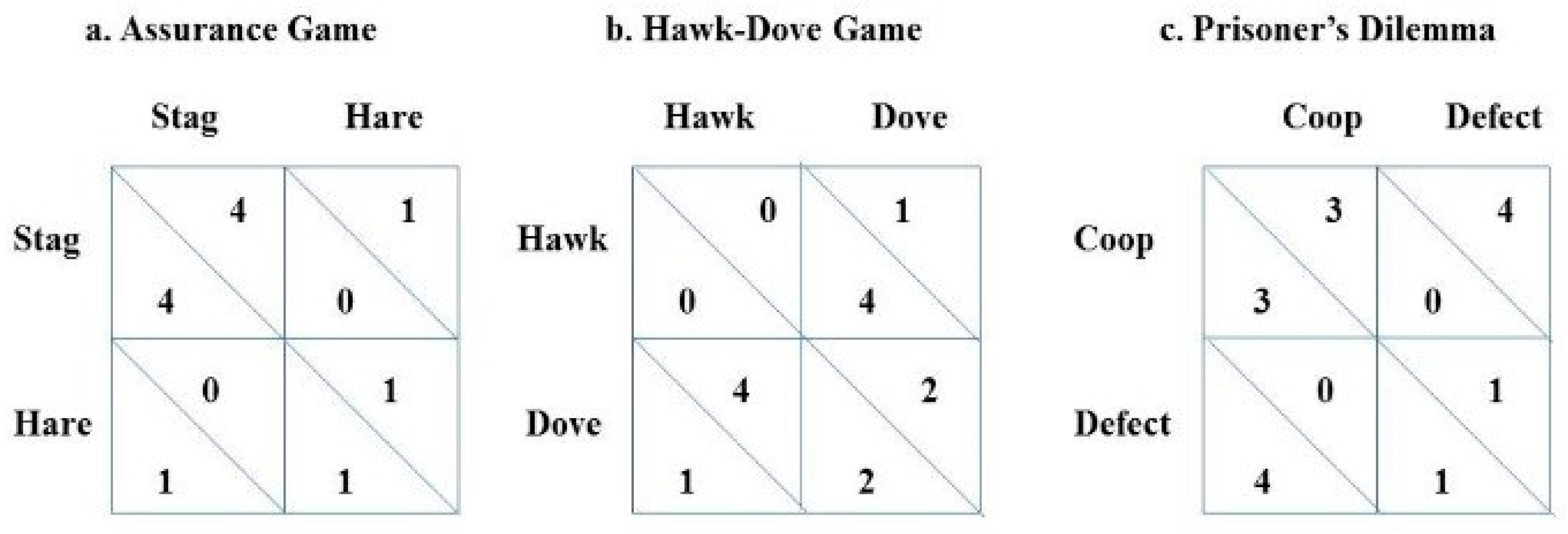
The findings suggest that Saimiri boliviensis may achieve coordination not through an understanding of interdependent decision-making but rather through associative learning of high- reward choices. Additionally, sex-based differences emerged, with female pairs demonstrating greater success in the AG, potentially reflecting species-specific social structures where females form stronger affiliative bonds.
The inability of squirrel monkeys to flexibly adjust their strategies in HDG and PDG highlights limitations in their cooperative decision-making. These results contribute to comparative cognition research by showing that species not known for cooperation may still coordinate under certain conditions, but their ability to engage in complex strategic interactions remains constrained. Further studies, particularly those involving computerized tasks, may help elucidate whether the observed behaviors are due to cognitive limitations or methodological constraints.
In this field of study, there have been several other studies in the literature delving into different perspectives, demonstrating the concern of some authors to identify patterns of behavior in cooperative games. One of these studies was carried out by El-Nasr et al. (2010), who analyzed recurring patterns among 60 participants in various games with this proposal of collaboration between members. As a result, it was possible to delve deeper into cooperative behaviors and measure them using a new metric called Cooperative Performance Metrics (CPMs).
From a business perspective, McCain (2008) aimed to fill a gap between the theory of cooperative games and the study of cooperative organizations, arguing that the theory can offer valuable tools for understanding and improving the functioning of cooperative organizations, especially by understanding and considering the importance of reciprocity.
The study by Churkin et al. (2021) analyzes how the power systems market and the concept of cooperative games can be implemented in cities in order to share costs and benefits between different agents such as energy companies, governments and consumers in order to guarantee an efficient and sustainable allocation of resources. An analysis from this perspective within game theory is essential as cities grow and the demand for energy increases, requiring coordinated investments and cooperation strategies between the various stakeholders involved in the sector.
2.14.1.2. Non-Cooperative Games
On the other hand, we have the so-called “Non-Cooperative Games” which, as Fujiwara- Greve (2015) argues, are characterized by the absence of any collaboration between people/institutions, as well as each of them making decisions independently without knowing the strategies of the other participants. We can conclude that, unlike cooperative games, there are no relationships of agreement, contracts or trust on the part of the members of this type of game.
As presented by Ritzberger (2002), some examples of this type of game include:
- Prisoner's Dilemma: a classic example illustrating the tension between individual and collective rationality. Two suspects are arrested and interrogated separately. The best individual strategy is to betray the other, even if cooperation would result in a lower sentence for both.
- Auctions: participants compete individually to acquire a good or service, without prior coordination. Each participant seeks to maximize their gain, i.e. obtain the good at the lowest possible cost.
- Oligopoly: Companies in an oligopolistic market make decisions about production and prices independently, taking into account the actions of their competitors, but without a formal cooperation agreement.
- Chicken Game: Two drivers drive towards each other. Whoever swerves first is considered the “loser”. Each player's decision is influenced by the expectation of the other's action, without prior communication.
These examples demonstrate how non-cooperative game theory provides conceptual tools for analyzing and predicting outcomes in situations where individual strategic interaction is paramount.
2.14.2. Symmetrical Games vs Asymmetrical Games
As highlighted by Cheng et al. (2004) in game theory, a game is classified as symmetrical if the players' payoffs depend exclusively on the strategies adopted and not on their identities. In other words, one player's payoff function can be obtained from another player's payoff function by simply exchanging roles. In a symmetrical game, if two players swapped strategies, the resulting payoffs would remain unchanged. A classic example of this category is the Prisoner's Dilemma, in which both participants face the same strategic options and obtain identical rewards under the same conditions.
On the other hand, a game is considered asymmetrical when at least one of the players has a different payoff function or a different set of strategies from the other participants. In this configuration, the exchange of roles between players can alter the payoffs and the strategic structure of the game. A paradigmatic example of an asymmetric game is the Hawk and Dove game, in which the players represent different types of agents with different incentives, leading to different strategies and equilibria. Murphy (1991) analyzed the limits between symmetry and asymmetry of “position” and information between communicator and audience within the field of public relations.
2.14.3. Perfect Information Games vs Imperfect Information Games
In game theory, the distinction between games of perfect information and games of imperfect information is fundamental for modeling and analyzing strategic decisions, from a simple betting ticket to public relations in companies and diplomatic issues. This classification is based on the degree of knowledge that players have about the actions taken by others throughout the game.
A game of perfect information is characterized by the fact that all players have complete knowledge of the history of decisions made up to the moment of their move. This implies that, at any point in the game, each player knows exactly what actions have been chosen by all the participants in the previous stages. As a result, there is no strategic uncertainty about the state of the game at the moment of decision making. Classic examples include games such as chess and tic-tac-toe, in which all the moves are observable by both players and there are no hidden elements or unknown randomness in the course of the game.
On the other hand, a game of imperfect information occurs when at least one of the players does not have complete access to the decision history of the other participants. This can happen, for example, when some actions are taken privately or when there are elements of the game that are not directly observable by all the players. This type of structure generates strategic uncertainty and can lead to the development of strategies based on expectations and beliefs about the actions of opponents. We can say that poker is a classic example of a game of imperfect information, since players don't know their opponents' cards and must make decisions based on partial information and strategic inferences as we have seen from Thorp (1966). For further information on this concept, we recommend visiting the works by Kreps and Wilson (1982) and Galliani (2012).
2.14.4. Symmetric Information
In symmetric information games, the information structure is characterized by the equivalence of knowledge between the players, where each participant has access to the same set of relevant information for making strategic decisions. As well explored by Hillier (1997), this informational symmetry implies that there are no information asymmetries that can confer competitive advantages on specific players, resulting in an environment of strategic interaction where decisions are based on a common set of knowledge.
The analysis of symmetric information games can be fundamental to understanding scenarios where transparency and equal access to information are crucial elements, such as in ideal competitive markets or in social interactions modeled on norms of fairness. Examples of games that employ the use of symmetric information include board games such as checkers and chess, soccer, horse races and, auctions, for example, in the sense that all participants have access to the same rules of the game.
2.14.5. Asymmetric Information
In game theory, asymmetric information emerges when players do not have the same set of relevant information for decision-making. This informational disparity can generate power imbalances and significantly influence the strategies and outcomes of games. Akerlof (1970), in his seminal study “The Market for ‘Lemons’: Quality Uncertainty and the Market Mechanism” vividly illustrates the consequences of asymmetric information in markets, while Greenwald and Stiglitz (1990) explore its implications for the theory of the firm.
Akerlof (1970) demonstrates how asymmetric information can lead to the collapse of markets, especially those characterized by uncertainty about the quality of the goods traded. In the used car market, for example, sellers have more information about the actual condition of vehicles than buyers.
This informational asymmetry creates a problem of adverse selection: sellers of low- quality cars called lemons are more likely to offer their vehicles on the market, while sellers of high-quality cars may be reluctant to do so, fearing that buyers won't be willing to pay the right price. Consequently, the market becomes dominated by “lemons”, crowding out good quality cars and, in extreme cases, leading to their disappearance. Akerlof formalizes this dynamic by showing how the demand curve can collapse due to uncertainty, resulting in an inefficient market.
Greenwald and Stiglitz (1990) expand the analysis of asymmetric information to the context of the theory of the firm. They argue that informational asymmetry between managers and investors can lead to financial constraints and affect the risk-taking behavior of firms. When investors do not have complete information about a company's prospects, they may demand a higher risk premium to provide capital. This additional risk premium can limit companies' access to financing, especially for riskier investment projects, even if these projects have a high return potential.
Information asymmetry can also influence the behavior of managers, who can be more risk-averse than shareholders, leading to sub-optimal investment decisions. Greenwald and Stiglitz (1990) highlight how asymmetric information can generate a variety of problems, including the inappropriate choice of projects, excessive risk aversion and the difficulty of monitoring managers' performance.
In short, both Akerlof (1970) and Greenwald and Stiglitz (1990) demonstrate that asymmetric information is a crucial factor in game theory and economic analysis. Information disparity between players can lead to inefficient results, such as the collapse of markets and sub- optimal investment decisions.
Beranek and Buscher (2024) examined and concluded that the impact of asymmetric information in the closed-loop supply chain is complex and can be influenced by factors such as the actual return rate and the power dynamics within the chain. The research also found that the retailer can compensate for the information disadvantage in most cases due to its position as Stackelberg's leader. In addition, the authors highlighted the importance of a deliberate search for cooperation between the players in order to deliver better results, both economically and ecologically.
In the context of sports betting, asymmetric information is a central element in the dynamic between bettors and sportsbooks. Information disparity manifests itself in several dimensions, from privileged access to data and analysis to the ability to interpret and react to market fluctuations. While sportsbooks enjoy a vast array of information and analytical tools to determine odds and manage risk, individual bettors may rely on less reliable sources or outdated information. This asymmetry of information can lead to sub-optimal betting decisions and an inadequate assessment of the risks involved by bettors.
The complexity of asymmetric information in sports betting is also exacerbated by the influence of market behavior. The actions of other bettors, in turn, can generate implicit information about the sporting event in question, influencing odds and betting lines.
Sportsbooks, aware of these dynamics, can adjust their offers to maximize their profits, exploiting the informational asymmetry between market participants.
Despite the great similarity between imperfect information and asymmetric information, we can say that imperfect information refers more to the lack of sufficient information available for “rational” decision-making, and asymmetric information refers more to the quantitative aspect, i.e. how much more information one player has than the other.
2.14.6. Repeated Games
As presented by Mertens (1990) and corroborated by Slantchev (2004) a repeated game occurs when the same game or a similar strategic structure is repeated over time, allowing players to learn and adjust their decisions based on previous experiences.
According to Sorin (2023) in this type of game, Aumann and Shapley's "Long-Term Competition—a game-theoretic analysis" (1994) utilizes repeated game theory to analyze sustained competitive interactions, notably in international relations, highlighting how the dynamic nature of these interactions enables strategies based on past behaviors and future expectations, including punishment and reward. Exploring both cooperative and noncooperative solution concepts, the paper emphasizes the Folk Theorem's significance in explaining the potential for diverse equilibria, including cooperative outcomes, in long-term settings, providing a framework for understanding strategic choices in contexts like arms races and negotiations by focusing on the temporal dimension of strategic interactions.
In sports betting, an example of repeated game can be observed in professional bettors who continuously participate in the betting market over several sports seasons. In this case, players can modify their strategies according to the previous performance of teams, the effectiveness of statistical models and even observation of the behavior of the betting market. In addition, the repetition of the game allows for the development of dynamic strategies, such as bankroll management and adapting to changes in the odds offered by sportsbooks. The study by Aumann et al. (1995), when considering an analysis of repeated games with imperfect information, provides us with rich content as a complement to this topic.
2.14.7. Positive Sum Games and Negative Sum Games
According to Klein (1991) and also corroborated by Brouwer (2016) a positive-sum game is characterized when the end result benefits all parties involved, that is, this scenario contrasts with the zero-sum paradigm, where one player's gain necessarily implies another's loss.
Cooperation and the creation of shared value are central characteristics of this type of game.
As Klein (1991) also points out, strategies that foster collaboration, innovation and the expansion of resources are crucial to achieving mutually advantageous results. The theory of positive-sum games, as we can see from Brouwer (2016) on Schumpeter's positive-sum game approach, has applications in various areas, such as economics, international relations and business management, where the search for “win-win” solutions can be fundamental to a company's growth and survival in the open market.
On the other hand, a negative-sum game is one in which the total sum of gains and losses across all players is less than zero. This implies that, by the end of the game, the overall pool of resources or benefits has diminished, leading to a scenario where all participants, in aggregate, experience a net loss. Usually, in these contexts, irrationality, lack of communication and the search for short-term advantages can lead to negative net results. Some examples of this category of games include armed conflicts, price wars and environmental crises, for example, in which we can see scenarios where the destruction of value outweighs individual gains. Through Warren's paper (2020) we can see a real example of a game that has been characterized as negative-sum in the financial market.
2.14.8. Zero-Sum Games
Let N be a finite set of players, with N={1, 2,..., n}. Each player i∈N has a set of strategies Si, where the strategy space of the game is given by the Cartesian product S = S1× S2 ×…× Sn.
We define a payoff function ui : S → for each player i, which associates a real value with the strategy profile s = (s1, s2,…, sn) ∈ S.
The game is called a zero-sum game if, for every strategy profile s∈ S, the sum of all players' payoffs is zero, i.e:
In the particular case of a two-player zero-sum game, where N ={1,2}, the payoffs are related by u1(s) + u2(s) = 0, implying that any gain by one player corresponds to an identical loss by the other.
Below we see the concept of minimax:
This result, known as von Neumann's Minimax Theorem (1928), states that, for two- player zero-sum games with finite strategy spaces, there is always an equilibrium in mixed strategies where both players minimize their maximum possible losses.
2.14.9. The Nash Equilibrium
The Nash Equilibrium is a fundamental concept in game theory, introduced by John Nash (1950), which describes a state in which no player can unilaterally improve their outcome by changing their strategy, as long as the other players keep their choices unchanged.
Let a strategic game be defined by a tuple (N, S, u), where:
N ={1, 2, ..., n} is the finite set of players;
Si is the set of strategies of player i;
S = S1× S2 × … × Sn is the game's strategy space;
ui : S → is the utility function of player i, associating a real payoff with each strategy profile s = (s1, s2, ..., sn).
A strategy profile:
is a Nash Equilibrium if, for every player i∈ N and for every alternative strategy si∈ Si:
As we can see, according to Griffin (2012) a Nash equilibrium occurs when no player can improve their payoff by unilaterally changing their strategy, assuming that the other players keep their strategies unchanged.
2.14.10. Nash Equilibrium in Mixed Strategies
If we allow players to choose strategies probabilistically, the concept can be extended to mixed strategies. Let Δ(Si) be the set of probability distributions over Si. A mixed strategy profile is a Nash Equilibrium in Mixed Strategies if, for every player i∈ N and for every alternative mixed strategy σi∈ Δ(Si):
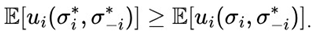
According to Bortolossi et al. (2017) this means that every finite game in which players can adopt mixed strategies has at least one Nash equilibrium. This result guarantees the existence of a point of stability in finite strategy games, in which no player has an incentive to deviate unilaterally, given that the others maintain their strategies.
2.14.11. Bayesian Equilibrium
Bayesian inference is a statistical method that updates the probability of a hypothesis as more evidence or information becomes available. In this method, Bayes' theorem is used to combine previous beliefs (a priori probabilities) with new evidence (data) to obtain updated beliefs (a posteriori probabilities). For a more in-depth look at this statistical topic, we recommend reading Smith (1984) in which the main points about Bayesian statistics are reviewed and discussed.
Myerson (1983) argues that a Bayesian equilibrium, sometimes also referred to in the literature as a Bayes-Nash equilibrium, developed by Harsanyi (1967) is a central concept in game theory, particularly when considering games with incomplete information. In a Bayes game, the players do not have complete information about the other players, but they do have beliefs - subjective probabilities - about the types of the other players. Bayesian equilibrium generalizes the concept of Nash equilibrium to games with incomplete information.
Let a game be G = ⟨N, A, u, μ⟩, where:
N = {1, 2,… , n} is the set of players.
A = A1× A2 × … × An is the set of possible actions, where Ai is the set of actions available to player i∈N
ui : A → is the utility function of player i, where ui(a) is the utility of player i when choosing action a∈ A
μi is the information or type of player i, represented by a random variable with probability distribution πi, which describes the player's uncertainty about the types of the other players.
We also denote the set of beliefs of player i about the types of the other players j∈N∖{i} by π-i, which is a probability distribution.
The Bayesian equilibrium is a vector of strategies σ = (σ1, σ2, ..., σn), where σi : μi → Ai is the strategy of player i and σ-i is the set of strategies of the other players. The equilibrium condition is that, for each player i, the strategy σi is rational given his belief πi about the type of the other players j∈ N∖{i}. For each player i and type μi∈ τi, the strategy σi(μi) should maximize the expected utility of player i, given the beliefs π-i and the strategies of the other players σ-i, i.e:
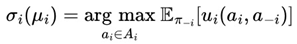
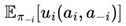 is the expected utility for player i when choosing action ai, given that the other players choose their actions a-i according to strategies σ-i, and that the probability distribution π-i reflects player i's beliefs about the types of the other players.
2.14.12. Dominant and Dominated Strategies
In game theory, according to Samuelson (1992) a dominant strategy is a course of action that yields the highest payoff for a player, regardless of the strategies chosen by other players.
When a player has a dominant strategy, it simplifies decision-making, as the optimal choice remains consistent across all possible scenarios. The presence of dominant strategies can lead to a unique outcome known as a dominant strategy equilibrium, where all players select their respective dominant strategies. This concept is fundamental in analyzing strategic interactions, as it identifies situations where rational players will inevitably converge on a particular set of actions.
Conversely, a dominated strategy is one that consistently provides a lower payoff compared to another available strategy, irrespective of the other players' choices. As Hofbauer and Weibull (1996) pointed out, rational players will always avoid dominated strategies, as they represent suboptimal decisions. The process of eliminating dominated strategies can simplify complex games by reducing the number of possible outcomes. In some cases, repeated elimination of dominated strategies can lead to a unique solution, known as the iterated dominance equilibrium. This method is particularly useful in games where players possess complete information and act rationally, allowing for the prediction of outcomes based on logical deduction.
2.14.13. Sports Betting and Game Theory
We can see that sports betting is part of some important categories within game theory, such as repeated games, games of imperfect information, zero-sum and “near-zero-game”, for example.
There are many debates and a not very clear consensus on the nature of sports betting, which is due to the analysis of this market from different angles. In their study, Levitt (2004) and Vizard (2023) classified sports betting as a zero-sum game because, just as in the financial market, there are two traders operating on each side and the profit of one consists of the loss of the other. Furthermore, in this market, there is no generation of value, so money only moves between the players with an intermediary (sportsbooks).
It is known that there are two categories in this sports betting market: the first consists of the bettor challenging the “House” and the odds offered by the sportsbooks, and the second category - commonly known as exchange - the bettors challenge each other. In principle, if we consider that the bettors model the market according to their convictions and the strategies they deem optimal, the game would be considered zero-sum. The problem is that according to the business model, sportsbooks, regardless of the category, whether traditionally or through the exchange, set a profit rate called vigorish. Therefore, regardless of the outcome, Sportbooks will always have a guaranteed income.
We can say that the exchange modality is a closer version of the zero-sum game in which we can classify this market as an almost zero-sum game and even a negative-sum game for the bettor in the long term due to the presence of vigorish.
3. While My Dice Gently Weeps
3.1. Victoria
Just as the Tupi Guarani language, Fort Orange from the Island of Itamaracá, a municipality in the state of Pernambuco, Brazil, inspired the name of the Itamaracá PRNG algorithm, Victoria also had its moments.
The Victoria methodology is named after the city of Victoria in British Columbia, Canada. This city is known for its appreciation of the natural world, as well as its artistic and technological atmosphere. It is named after Queen Victoria of the United Kingdom, who left a strong legacy and commitment to the development of science, marking, for example, a golden age for Statistics through various discoveries that today shape the world around us.
Furthermore, when we're in a game, it is natural to want the ultimate goal, which is victory. So it is a reflection that the player, mathematically and statistically, will always have the advantage over the house in the medium and long run, regardless of any positive or negative results that occur along the way.
As we can see from Figure 20, we can find different configurations and different results. We can say a configuration belongs to 94%, for example, if over the course of 100 FVs (Future Values) it has a maximum of 6 FVs with a result that is usually modestly negative over the long term. Therefore, the other 94 FV s contain positive results, indicating profitability in all of them.
Figure 20.
Configurations of φ, j and k separated by different categories.
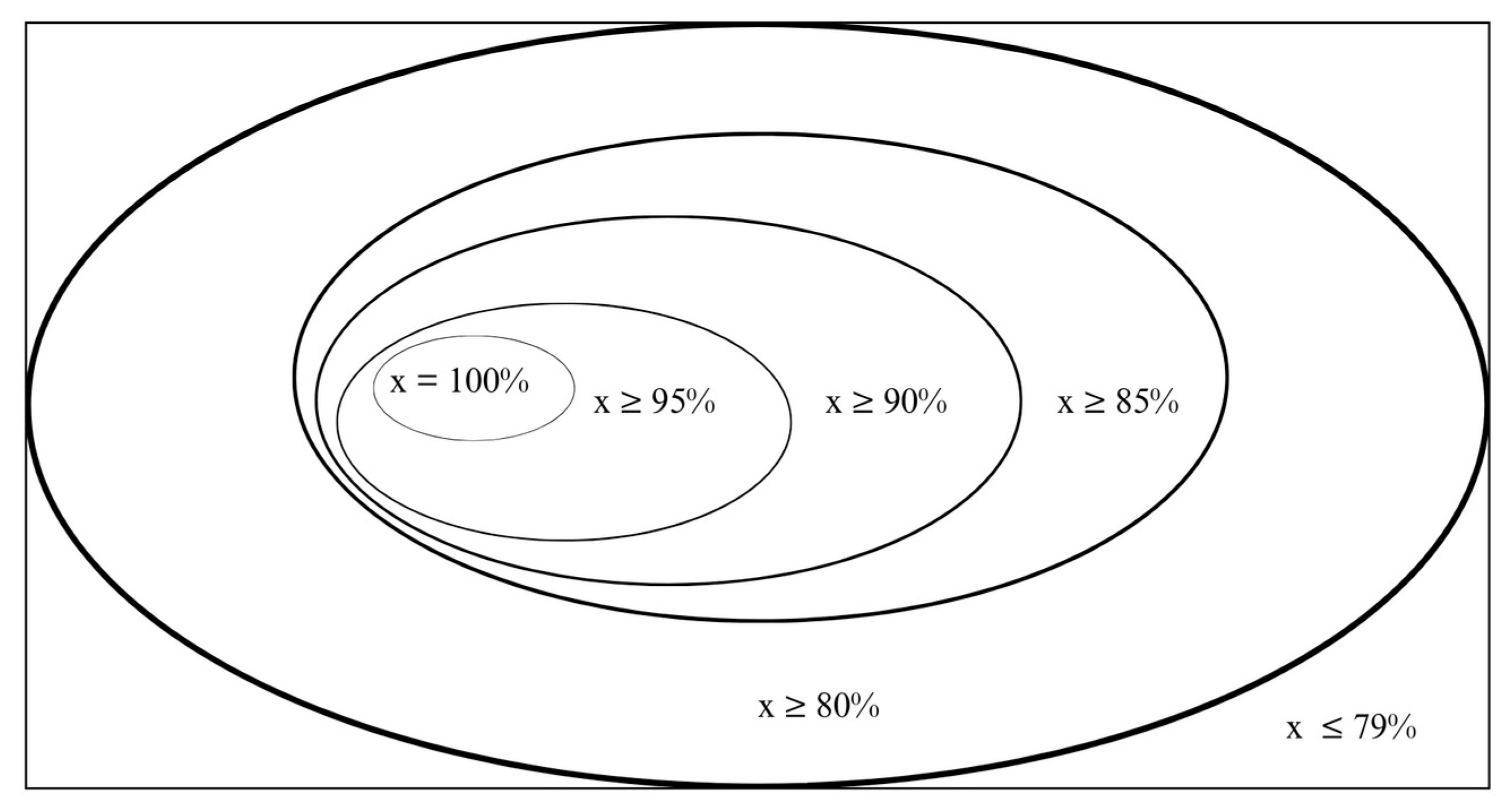
It is known that in each standard Future Value (FV) approximately 10,000 games are theoretically expected. However, in practice, the actual amount of games will probably vary between 4,800 and 7,000 games depending on the settings chosen for a bettor to fulfill a complete FV containing all of his expected 100 Intermediate Blocks (IBs) and Small Blocks (jn).
It is clear to see that the closer to 100% a given configuration is, the less games and, consequently, time the bettor will have to play in order to mathematically eliminate any risks inherent in random noise, meaning that the most desirable thing is to identify a configuration that, if not 100%, is always statistically close to 100%.
Considering that today we have made significant progress in robotization models through machine learning and data mining, configurations that statistically offer us at least 94% positive FVs still seem viable for possible practical projects of this theorizing. In fact, other configurations such as those that converge to at least the 80% and 85% category, for example, could also present interesting costs/benefits, provided that the bettor is willing to take on more risk. All of these definitions will be discussed in more detail throughout this study.
Victoria is based partly on the premise that advanced statistics and part of “tamed” randomness can offer sustained strategic advantage, even in games considered to be zero-sum. Fisher (1955) discusses the role of statistics in rational decision-making and how the correct use of inference can increase the probability of success in random systems.
In addition, the Victoria inspired by Stirling numbers in duplicate data analysis, anchored in the foundations of convergence in probability, also has interesting interconnections with the basic premises of Renewal Theory, specifically through the paper of Cox (1962). This theory is an extension of stochastic processes that studies times between successive events in random systems, especially in contexts such as:
- queues and arrivals of customers in waiting processes
- failure and maintenance of engineering systems
- evolution of patterns over time in Markov chains.
The central idea of renewal theory is that there are statistical patterns in the times between events, allowing partial predictability in systems that, at first glance, may seem purely random, suggesting to us that structurable patterns can emerge from these chaotic processes.
Hubbell (2001) presented “The Unified Neutral Theory of Biodiversity and Biogeography” in which the author sought to explain patterns of biodiversity and biogeography based on principles of neutrality between species, where all species are considered ecologically equivalent (random) in their chances of birth, death, dispersal and speciation, for example.
Despite their randomness, it is noticeable that on a large scale, patterns can emerge due to cumulative interactions. In this sense, while analyzing complex biological and ecological systems, it also leads us down similar paths proposed by Cox (1962) as well as in the theorizing behind Victoria and the Victoria-Nash Asymmetric Equilibrium (VNAE).
Below is Victoria's general formulation:
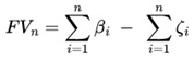 where,
jn =[(S0 φ k– S0) βi] – S0 ζi
φ = odd / probability of success of the event k = Time Period
S0 = Initial Value (fixed value used for each independent event)
β = "Success" blocks. That is, the cost/benefit ratio compared to the investment in each stake in each n game is positive and there is some profit.
ζ = "Failure" blocks. That is, the cost/benefit ratio compared to the investment in each stake iin each n game is negative and there is some loss.
We can say that the Victoria algorithm is based on the perspective of “blocks” and/or “hierarchy” for the sake of clarity. Below are some fundamental definitions:
p : probability, odd
S0 : initial value, stake
m : Number of Small Blocks (jn) in an Intermediate Block (IB)
k : number of k independent events
IB : Intermediate Block
βi : number of successful Small Blocks in an IB. ζi : number of Small Blocks of failure (ζi = m - βi) wβ : gain associated with a successful Small Block
lζ : loss associated with a small block of failure (ζ).
Within an Intermediate Block (IB) the final result of gain or loss will depend on the number of successful (β) or unsuccessful (ζ) blocks.
Total gain from successful Small Blocks (β) can be represented by:
Wβ = β ּ wβ
Total loss from Small Blocks of failure (ζ) can be represented by:
Lζ = ζ ּ lζ = (m – β) ּ lζ
Next, we'll look at the net result of any given Intermediate Block (IB):
RIB = Wβ – Lζ
RIB = (β ּ wβ ) - [(m - β) ּ lζ ]
RIB = β ּ ( wβ + lζ ) - m ּ lζ
Since in this scenario we are dealing with a binary option, i.e. at the end of an n sequence with k random events whose outcome will define whether a block will be considered a success (returning some profit) or a failure (returning a negative value), we can consider that they follow a binomial distribution:
β ~ Binomial (n = m, p = P(β))
ζ ~ Binomial (n = m, p = P(ζ))
We can define the expected value of the result in an IB:
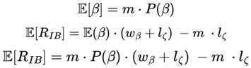
The general formula for the variance of the result of an Intermediate Block (IB) is:

Below, we'll see that the Future Value (FV) consists of the sum of all the results of the Small Blocks of Success (β) or Failure (ζ) present within each Intermediate Block (IB):
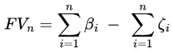
Next, we can see the expected value and the general formula that shows the difference between the total sum of gains and losses over a Future Value (FV):
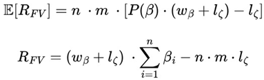
3.1.1. Design of an Intermediate Block (IB)
Table 7 shows the standard design of an Intermediate Block (IB):
Table 7.
Design of an Intermediate Block (IB).
| j1 | j2 | j3 ... jn |
|---|---|---|
| k1 | k1 | k1 k1 |
| k2 | k2 | k2 k2 |
| k3 | k3 | k3 k3 |
| ... | ... | ... ... ... |
| kn | kn | kn kn |
The product of jn and kn must be equal to or something close to 100. Knowing this information, we can say there will be several n possible combinations of jk. However, it should be clear after this first choice of j, and k there will also be the parameter φ considered “optimal”. This is what we'll see in the next topic.
Assuming that, with φ = 1.60 as a reference, we choose the following parameters j =16 and k = 6, we will have the following Intermediate Block (IB):
Table 8.
Example configuration with j = 16 and k =6.
| j1 | j2 | j3 | j4 | j5 | j6 | j7 | j8 | j9 | j10 | j11 | j12 | j13 | j14 | j15 | j16 |
|---|---|---|---|---|---|---|---|---|---|---|---|---|---|---|---|
| k1 | k1 | k1 | k1 | k1 | k1 | k1 | k1 | k1 | k1 | k1 | k1 | k1 | k1 | k1 | k1 |
| k2 | k2 | k2 | k2 | k2 | k2 | k2 | k2 | k2 | k2 | k2 | k2 | k2 | k2 | k2 | k2 |
| k3 | k3 | k3 | k3 | k3 | k3 | k3 | k3 | k3 | k3 | k3 | k3 | k3 | k3 | k3 | k3 |
| k4 | k4 | k4 | k4 | k4 | k4 | k4 | k4 | k4 | k4 | k4 | k4 | k4 | k4 | k4 | k4 |
| k5 | k5 | k5 | k5 | k5 | k5 | k5 | k5 | k5 | k5 | k5 | k5 | k5 | k5 | k5 | k5 |
| k6 | k6 | k6 | k6 | k6 | k6 | k6 | k6 | k6 | k6 | k6 | k6 | k6 | k6 | k6 | k6 |
As you can see from then on there will be 100 Intermediate Blocks ( IB), each of which will contain 16 Small Blocks (Jn), each containing 6 independent events with a probability of success of 62.5%, giving a total of 96 independent events with equal probability p(x) of running.
Let's take the following data as an example:
φ (Odd) = 1.60
k = 6
j = 16
jk = 96
IBn =[(S0 φ k– S0) β] – S0 ζ
IB1 = [10 * 1.60 ⁶ – 10) 2] - 10 * 14
IB1 = 175.54
We got $ 175.54 as a result. In this sense, we can say we have a positive value, with two small blocks of success and 14 small blocks of failure.
In another scenario, as the Monte Carlo simulation has shown to be promising, we can use the following parameters as a reference: φ = 1.04; j = 3 and k = 33. We will then have the following table.
Table 9.
Example configuration with j = 3 and k = 33.
| j1 | j2 | j3 |
|---|---|---|
| k1 | k1 | k1 |
| k2 | k2 | k2 |
| k3 | k3 | k3 |
| k4 | k4 | k4 |
| k5 | k5 | k5 |
| k6 | k6 | k6 |
| k7 | k7 | k7 |
| k8 | k8 | k8 |
| k9 | k9 | k9 |
| k10 | k10 | k10 |
| k11 | k11 | k11 |
| k12 | k12 | k12 |
| k13 | k13 | k13 |
| k14 | k14 | k14 |
| k15 | k15 | k15 |
| k16 | k16 | k16 |
| k17 | k17 | k17 |
| k18 | k18 | k18 |
| k19 | k19 | k19 |
| k20 | k20 | k20 |
| k21 | k21 | k21 |
| k22 | k22 | k22 |
| k23 | k23 | k23 |
| k24 | k24 | k24 |
| k25 | k25 | k25 |
| k26 | k26 | k26 |
| k27 | k27 | k27 |
| k28 | k28 | k28 |
| k29 | k29 | k29 |
| k30 | k30 | k30 |
| k31 | k31 | k31 |
| k32 | k32 | k32 |
| k33 | k33 | k33 |
It can be seen, from then on, we will have 100 Intermediate Blocks (IB), each containing 3 Small Blocks (j) with each containing 33 independent events (k) with a probability of success of 96.15%, giving a total of 99 independent events with equal probability p(x) of occurring.
3.1.2. Analysis of the Parameters φ, j, k and the Profit vs. Loss Curve
We can say that the parameter φ corresponds to the value of the odds offered by sportsbooks through an expected probability analysis for each independent event k. Therefore, the parameter k is nothing more than the number of n independent events in which the user will repeat using the same odds φ multiplied by the stakes accumulated over time, just as in the general formula for compound interest in the field of financial mathematics.
Through this theorizing, we can expect a great deal of sensitivity regarding the choice of variation in the profit curve as a function of the other variables such as stake, odds containing the probability of success as well as the design of the intermediate blocks through the choice of j and k.
3.1.3. Choosing the Parameters φ, j and k Considered “optimal”
The choice of the parameters φ, j and k considered optimal should be made using trial and error through monte carlo simulation. One way of saying that these parameters have been validated is if the final results from the sum of all the Small Blocks (jn) and Intermediate Blocks (IB), with their cost-benefit ratio compared to all the investment made during the process, show positive final results, i.e. indicating a guaranteed profit for the player regardless of what happens during the sequence.
There are countless possible combinations, even unknown to the author himself at the time of writing this article.
Below are some values of φ, k and j which could be promising for being in the 90%, 95% or even 100% category, regardless of the scenario with n independent event sequences tending to infinity.
Table 10.
Some potential configurations for good long-term results.
| φ | k | j |
|---|---|---|
| 1.02 | 25 | 4 |
| 1.02 | 33 | 3 |
| 1.02 | 50 | 2 |
| 1.03 | 33 | 3 |
| 1.03 | 50 | 2 |
| 1.03 | 100 | 1 |
| 1.04 | 33 | 3 |
| 1.04 | 50 | 2 |
| 1.06 | 33 | 3 |
| 1.07 | 20 | 5 |
| 1.07 | 25 | 4 |
| 1.08 | 25 | 4 |
| 1.10 | 12 | 8 |
| 1.11 | 16 | 6 |
| 1.11 | 20 | 5 |
| 1.12 | 16 | 6 |
| 1.14 | 14 | 7 |
| 1.16 | 12 | 8 |
| 1.4 | 7 | 14 |
| 1.6 | 6 | 16 |
| 1.8 | 5 | 20 |
| 2 | 4 | 25 |
| 3 | 4 | 25 |
| 4 | 3 | 33 |
3.2. Simulating the Application of the Victoria Formula in Different Expected Scenarios
For practical demonstration purposes, let's consider the following configurations:
φ= 1.03
k= 33
j=3
jk= 99 ~ 100.
We can see that with φ = 1.03, we can expect each k independent event to have a 97.09% probability of success. We can also see there will be 33 independent events and 3 small blocks jn totaling a maximum of 99 independent events expected to occur in each Intermediate Block (Ibn).
In order to analyze whether certain configurations are promising or not in terms of the player always having an advantage over the sportsbooks in sports betting, we can simply apply the monte carlo simulation technique and continuously analyze sequences of random numbers.
In this example, we used the Random.org platform - a source that generates true random numbers - to generate a sequence of numbers ranging from 1 to 1,000 with a uniform distribution.
As we can see from Table 11, the player would have bet $10 on each Small Block and had a negative result, a loss, of -$30 on this particular hypothetical Intermediate Block, since the player would have had failures at k = 25 on Small Block j1, k = 7 on Small Block j2 and k = 11 on Small Block j3 since x ≤ 29, which classifies these numbers within the range of probabilities expected for the player to lose the bet.
Table 11.
Parameters φ = 1.03, j = 3, k = 33.Example with 0 Success Blocks (β) and 3 Failure Blocks (ζ). Random numbers between 1 and 1000 generated by Random.Org. jn =[(S0 φ k– S0) β] – S0 ζ; j1 = [ 10 * 1.03 33 – 10 ) 0] - 10 * 3 j1 = - $ 30.
Table 11.
Parameters φ = 1.03, j = 3, k = 33.Example with 0 Success Blocks (β) and 3 Failure Blocks (ζ). Random numbers between 1 and 1000 generated by Random.Org. jn =[(S0 φ k– S0) β] – S0 ζ; j1 = [ 10 * 1.03 33 – 10 ) 0] - 10 * 3 j1 = - $ 30.
| k | j1 | j2 | j3 |
|---|---|---|---|
| 1 | 646 | 138 | 441 |
| 2 | 731 | 915 | 423 |
| 3 | 245 | 895 | 754 |
| 4 | 489 | 875 | 566 |
| 5 | 852 | 741 | 41 |
| 6 | 371 | 528 | 811 |
| 7 | 972 | 12 | 694 |
| 8 | 275 | 421 | 437 |
| 9 | 108 | 72 | 102 |
| 10 | 711 | 531 | 898 |
| 11 | 376 | 928 | 28 |
| 12 | 332 | 677 | 324 |
| 13 | 589 | 893 | 824 |
| 14 | 699 | 910 | 474 |
| 15 | 209 | 826 | 768 |
| 16 | 660 | 479 | 981 |
| 17 | 243 | 804 | 421 |
| 18 | 240 | 13 | 990 |
| 19 | 622 | 498 | 286 |
| 20 | 466 | 398 | 870 |
| 21 | 628 | 839 | 481 |
| 22 | 321 | 767 | 3 |
| 23 | 344 | 217 | 853 |
| 24 | 646 | 717 | 940 |
| 25 | 23 | 67 | 736 |
| 26 | 994 | 543 | 115 |
| 27 | 740 | 43 | 516 |
| 28 | 624 | 151 | 733 |
| 29 | 914 | 665 | 491 |
| 30 | 330 | 600 | 894 |
| 31 | 344 | 939 | 725 |
| 32 | 22 | 219 | 281 |
| 33 | 723 | 69 | 814 |
As we can see from Table 12, the player would have bet $10 on each Small Block and would have had a negative result, a loss, of - $3.48 on this particular hypothetical Intermediate Block, since the player would have had failures at k = 12 on Small Block j1, and, k = 2 on Small Block j3 since x ≤ 29 which classifies these numbers within the range of probabilities expected for the player to lose the bet and consider it a small block of failure. According to the same table, we had one small block of success (β) and 2 small blocks of failure (ζ).
Table 12.
Parameters φ = 1.03, j = 3, k = 33.Example with 1 Success Block (β) and 2 Failure Blocks (ζ). Random numbers between 1 and 1000 generated by Random.org. IBn =[(S0 φ k– S0) β] – S0 ζ; IB1 = [ 10 * 1.03 33 – 10 ) 1] - 10 * 2 IB1 = - $ 3.48.
Table 12.
Parameters φ = 1.03, j = 3, k = 33.Example with 1 Success Block (β) and 2 Failure Blocks (ζ). Random numbers between 1 and 1000 generated by Random.org. IBn =[(S0 φ k– S0) β] – S0 ζ; IB1 = [ 10 * 1.03 33 – 10 ) 1] - 10 * 2 IB1 = - $ 3.48.
| k | j1 | j2 | j3 |
|---|---|---|---|
| 1 | 724 | 598 | 449 |
| 2 | 432 | 572 | 17 |
| 3 | 630 | 216 | 190 |
| 4 | 511 | 697 | 617 |
| 5 | 154 | 375 | 187 |
| 6 | 774 | 828 | 907 |
| 7 | 272 | 548 | 813 |
| 8 | 757 | 466 | 646 |
| 9 | 984 | 39 | 408 |
| 10 | 990 | 507 | 627 |
| 11 | 248 | 651 | 965 |
| 12 | 23 | 566 | 934 |
| 13 | 247 | 406 | 855 |
| 14 | 75 | 643 | 585 |
| 15 | 685 | 151 | 630 |
| 16 | 720 | 363 | 993 |
| 17 | 686 | 416 | 883 |
| 18 | 433 | 742 | 528 |
| 19 | 986 | 133 | 826 |
| 20 | 445 | 592 | 8 |
| 21 | 605 | 163 | 91 |
| 22 | 255 | 332 | 686 |
| 23 | 874 | 818 | 969 |
| 24 | 843 | 878 | 505 |
| 25 | 286 | 811 | 905 |
| 26 | 794 | 198 | 294 |
| 27 | 611 | 947 | 840 |
| 28 | 496 | 252 | 255 |
| 29 | 855 | 878 | 610 |
| 30 | 981 | 487 | 773 |
| 31 | 472 | 511 | 847 |
| 32 | 581 | 633 | 501 |
| 33 | 138 | 968 | 921 |
Table 13.
Parameters φ = 1.03, j = 3, k = 33. Example with 2 Success Blocks (β) and 1 Failure Block (ζ). Random numbers between 1 and 1000 generated by Random.org; IBn =[(S0 φ k– S0) β] – S0 ζ; IB1 = [ 10 * 1.03 33 – 10 ) 2] - 10 * 1 IB1 = $ 23.05.
Table 13.
Parameters φ = 1.03, j = 3, k = 33. Example with 2 Success Blocks (β) and 1 Failure Block (ζ). Random numbers between 1 and 1000 generated by Random.org; IBn =[(S0 φ k– S0) β] – S0 ζ; IB1 = [ 10 * 1.03 33 – 10 ) 2] - 10 * 1 IB1 = $ 23.05.
| k | j1 | j2 | j3 |
|---|---|---|---|
| 1 | 16 | 604 | 956 |
| 2 | 279 | 718 | 517 |
| 3 | 52 | 283 | 291 |
| 4 | 797 | 746 | 265 |
| 5 | 915 | 613 | 226 |
| 6 | 310 | 651 | 903 |
| 7 | 224 | 699 | 716 |
| 8 | 541 | 987 | 905 |
| 9 | 382 | 40 | 243 |
| 10 | 347 | 458 | 286 |
| 11 | 339 | 957 | 744 |
| 12 | 187 | 248 | 33 |
| 13 | 380 | 731 | 806 |
| 14 | 642 | 485 | 489 |
| 15 | 432 | 396 | 66 |
| 16 | 886 | 929 | 548 |
| 17 | 420 | 158 | 141 |
| 18 | 885 | 395 | 488 |
| 19 | 747 | 282 | 164 |
| 20 | 207 | 661 | 643 |
| 21 | 680 | 662 | 573 |
| 22 | 314 | 931 | 794 |
| 23 | 451 | 780 | 943 |
| 24 | 914 | 587 | 908 |
| 25 | 833 | 235 | 394 |
| 26 | 608 | 321 | 942 |
| 27 | 909 | 637 | 548 |
| 28 | 957 | 181 | 885 |
| 29 | 95 | 217 | 918 |
| 30 | 713 | 693 | 690 |
| 31 | 310 | 158 | 68 |
| 32 | 759 | 60 | 562 |
| 33 | 925 | 689 | 624 |
Above, we can see that within the hypothetical Intermediate Block (IB) in Small Blocks (jn) we had 2 Success Blocks (β), i.e. we had all 33 winning events consecutively. On the other hand, we had what amounts to 1 Failure Block(ζ), i.e. in the course of these 33 consecutive events scheduled to occur at some point (k = 1; j1). As a result, we had an Intermediate Block with a positive result of $23.05.
As we can see from Table 14, the player would have bet $10 on each Small Block and had a very positive result of $49.57 on this particular hypothetical Intermediate Block, since the player would not have had any Small Block failures, i.e. with any event containing any values x ≤ 29.
Table 14.
Parameters φ = 1.03, j = 3, k = 33.Example with 3 Success Blocks (β) and 0 Failure Blocks (ζ). Random numbers between 1 and 1000 generated by Random.Org. IBn =[(S0 φ k– S0) β] – S0 ζ; IB1 = [ 10 * 1.03 33 – 10 ) 3] - 10 * 0 IB1 = $ 49.57.
Table 14.
Parameters φ = 1.03, j = 3, k = 33.Example with 3 Success Blocks (β) and 0 Failure Blocks (ζ). Random numbers between 1 and 1000 generated by Random.Org. IBn =[(S0 φ k– S0) β] – S0 ζ; IB1 = [ 10 * 1.03 33 – 10 ) 3] - 10 * 0 IB1 = $ 49.57.
| k | j1 | j2 | j3 |
|---|---|---|---|
| 1 | 535 | 976 | 902 |
| 2 | 728 | 653 | 275 |
| 3 | 628 | 836 | 632 |
| 4 | 883 | 683 | 538 |
| 5 | 76 | 521 | 939 |
| 6 | 74 | 853 | 222 |
| 7 | 420 | 762 | 656 |
| 8 | 807 | 385 | 905 |
| 9 | 60 | 732 | 692 |
| 10 | 241 | 527 | 177 |
| 11 | 396 | 841 | 494 |
| 12 | 337 | 604 | 914 |
| 13 | 621 | 169 | 202 |
| 14 | 35 | 40 | 785 |
| 15 | 86 | 213 | 961 |
| 16 | 113 | 996 | 251 |
| 17 | 829 | 800 | 68 |
| 18 | 755 | 797 | 30 |
| 19 | 289 | 519 | 543 |
| 20 | 317 | 432 | 570 |
| 21 | 283 | 25 | 314 |
| 22 | 366 | 166 | 745 |
| 23 | 168 | 911 | 646 |
| 24 | 511 | 650 | 90 |
| 25 | 642 | 548 | 313 |
| 26 | 651 | 638 | 931 |
| 27 | 273 | 736 | 978 |
| 28 | 919 | 296 | 508 |
| 29 | 378 | 360 | 425 |
| 30 | 238 | 545 | 402 |
| 31 | 966 | 816 | 599 |
| 32 | 199 | 551 | 882 |
| 33 | 326 | 560 | 507 |
3.3. The Theater of Dreams
Alice and Bob go together to a theater in their city to have some fun. It is known that there are 5 theatrical plays that show how to beat the house using statistics and randomness. Enthusiastic, they are both eager to see not just one but all the performances, no matter if they will stay inside for hours. Below is a list of all the plays that Alice and Bob will be seeing at the Theater of Dreams:
- Play I: Beating the house x% of the time and mathematically overcoming any possible losses along the way
- Play II: Beating the house x% of the time using some margin of advantage for the player and mathematically overcoming any possible losses along the way.
- Play III: Beating the house x% of the time"
- Play IV: Beating the house x% of the time using some margin of advantage for the player
- Play V “Beacon Hill Park”: Beating the house 100% of the FVs using the Victoria formula (without considering any advantages for the bettor, just that the odds are “fair”) by identifying ideal parameters that always converge to 100%. This is the “singularity point”, an open question in this research.
3.3.1. Play I: Beating the House x% of the Time and Mathematically Overcoming Any Possible Losses Along the Way
The couple realized during this first presentation that the Victoria formula has “almost mathematically perfect” possibilities for gains as there are configurations of φ, j, and k that allow statistical convergence to be greater than or equal to x% close to 100% positive FVs, such as 92%, 94%, and 97%.
In this play, it is presented on stage by the actors that even if it is not always 100% positive, if the category of the configuration is relatively close to this value, we can simply use positive mathematical expectation as well as a time period t and convergence in probabilities to our advantage.
If we consider, for example, that a given configuration of φ, j, and k has a maximum convergence of negative FVs of 4%, we can classify it as belonging to the 96% category, that is, with at least 96 positive FVs out of a total group of 100 FVs, so that in order to mathematically eliminate any possible risk of loss, all Alice and Bob have to do instead of betting a total of 4 FVs is consider betting a total of at least 5 FVs or more. This means that, as we increase the number of k independent events, which results in an increasing number of each Small Block (jn); Intermediate Blocks (IB) and even Future Values (FV), we say that the probability of having FVs with a negative outcome tends to zero.
Still on the previous example, it is known that on average the chosen configuration belonging to the 96% category will have approximately 98 positive FVs and 2 negative FVs. Furthermore, we know that Alice and Bob will have to bet approximately 5,500 games on each Future Value (FV). Based on this information, this means that from k independent event number 22,001, the couple will have mathematically eliminated all possible forms of loss considering the worst possible scenarios, such as having 4 sequences of FVs with negative results, which gives us a probability of (0.04 4 = .000256%) and the profit from that moment on will be ensured by the law of large numbers.
Section 3.4 of this study will present a theorem and a mathematical proof of what was pointed out in Play I presented at the Theater of Dreams.
3.2.1. Play II: Beating the House x% of the Time Using Some Margin of Advantage for the Player and Mathematically Overcoming Any Possible Losses Along the Way
As with Moya's (2012) approach of employing a margin of advantage for the bettor, Alice and Bob realized that by adding this element of advantage instead of simply the ‘fair odds’ offered by the sportsbooks, in rationally logical terms, we can expect that, for example, depending on the advantage established by the bettor over the sportsbook in so-called value bets, a set of configurations that could converge on 94%, for example, could easily get even closer to 100% in terms of the number of FVs with positive results.
If we take the example of a configuration with φ = 1.04, j = 3, and k = 33, for example, we have a probability of success of 96.15%. Let's also consider that after analyzing market inefficiencies, the odds were “fair” and now Bob would like to apply a margin of advantage over the house by considering φ = 1.03, j = 3, k = 33 as reference values for each Small Block (jn) to be considered successful or not, resulting in a probability of success of 97.09%. This difference of .94% added to the fact that the multiplicative factor of φ = 1.04 will return an even more significant positive net value than would naturally be the case with φ = 1.03, we can say that Bob, as well as being backed by a strong statistical analysis, will also have a small but interesting advantage against the house.
As we can see, if an advantage is placed against the house, it tends to exponentially decrease the time (understood as the number k independent events) needed to make it mathematically possible for the bettor to always make a profit against the house, regardless of all the negative results along the way.
In this sense, if, of course, a certain configuration belongs to the 95% category (understood as 95 out of 100 FVs with positive final values), it could easily come close to always being 100%. Under the same reasoning, if a certain configuration belongs to the 97% category, we could, by applying x% advantage to the bettor, always get a positive result over 100 FVs. In this case, the point of singularity could be reached by using Victoria plus a margin of advantage for the player.
To illustrate the practical impact of a 95% positive convergence configuration in the Victoria methodology, let's consider a hypothetical example in which each Future Value (FV) has a 95% chance of generating a positive result and only a 5% chance (in the worst case scenario) of being negative. In a set of 100 simulated FVs, this implies that, statistically, at least 95 FVs will tend to be positive and, at most, 5 FVs could result in negative values.
We can convert this probabilistic scenario into a design similar to that of a lottery, where the player fills in a ticket with 5 numbers between 1 and 100. In this case, numbers equal to or greater than 96 are considered “losing numbers”, resulting in negative FVs. The probability of the worst-case scenario occurring - that is, getting exactly 5 consecutive negative FVs within a set of 100 FVs - can be calculated as a compound probability:
in other words, the chance of facing a sequence of 5 consecutive losses in a 95% efficient configuration is only .00003125% - an extremely small value, indicating a rare but still possible event.
P(5 consecutive negative FVs) = 5% × 5% × 5% × 5% × 5% = (0,05)5 = .00003125%
On the other hand, if we consider a sequence of 5 FVs and we have 3 FVs or 4 FVs with some negative final result, indicating some degree of loss for the bettor, despite this - the other 2 FVs or just one positive FV - still tend to provide final values with profits substantially higher than the losses that occurred, so the bettor can still come out with a profit depending on the configuration of φ, j and k chosen.
3.3.3. Play III: Beating the House x% of the Time"
After the first three plays, Alice and Bob decided to go outside for a while to a kiosk outside the theater and began to reflect on everything they had experienced in that environment full of numbers and statistical magic, above all reflecting on the third play.
Another common scenario for expecting profits and beating the house is through the simple approach of the Victoria model and its respective belonging categories. If a given configuration of φ, j, and k converges to 85%, 90% or 97%, this means that we can expect to obtain, in the worst-case scenario, 15, 10 and 3 negative FVs, respectively, in each group of 100 FVs.
Let's still consider the previous examples. At this point, when the victorian bettor enters the market and puts the Victoria formula into practice, he can expect that the odds of him coming out with a positive FV will probably be something close to an average of 92.5%, 95% and 98.5%, respectively. Under the same reasoning, the bettor is also aware that these certain configurations are “almost perfect” and can present a very interesting cost/benefit ratio.
At this point, unlike plays I and II, where the aim is to mathematically eliminate all possibilities of losses (although this is relatively low and rare), this bettor is willing to take a small risk of getting sequences that could turn negative. As we saw in the previous sections, even if the bettor gets a few sequences of negative FVs, with the remaining positive FVs - depending on the settings chosen - the bettor can still make a satisfactory profit.
3.3.4. Play IV: Beating the House x% of the Time Using Some Margin of Advantage for the Player
The couple return to the Theater of Dreams to watch a new play and look forward to the long-awaited final performance. It is known that in Play IV, the idea is basically the same as in Play II, however, the main difference lies in the fact that in Play II the aim is to mathematically eliminate any possible loss when applying the Victoria model as well as adding any possible margin of advantage if the bettor wishes.
In Play IV, the margin of advantage sought by the bettor does not necessarily aim to always achieve 100 positive FVs out of all possible 100 FVs, but rather to apply that advantage to simply be closer to 100%.
This issue can become clearer if Alice and Bob, for example, find a certain configuration of φ, j and k that always converges to at least a category of 88% which, with an x% advantage applied to the player (if they wish and it is feasible to do so), can mean that instead of converging to this normal value expected by Victoria, it can converge to a new category, such as 94%. As a result, the objective in these cases could be to take advantage of the average cost/benefit presented in each positive FV of this initial category, which with an x% advantage not only increases the average profit expected in each FV, but also tends to considerably reduce the number of expected games.
3.3.5. Play V: Beacon Hill Park (Singularity Point)
In this final play, set in Beacon Hill Park, Alice and Bob are asked to find a “singularity point”, that is, an optimal configuration in the Victoria formula (without taking into account any margins of advantage for the bettor) that mathematically demonstrates that there will always be FVs with 100% positive results out of 100 FVs in a row, regardless of the time lapse. This is probably a question that will remain open when we talk about the Victoria methodology.
Determining these values would be fundamental in the sense that both have a smaller number of possible games to bet on and, consequently, become very viable in practice because they require less time. If we were to find these optimum configurations belonging to the singularity point, a Victorian punter, for example, would only have to hope to play 'only' between 4,800 and 7,000 games at most to mathematically secure some positive value. Surely, if we can prove it in the future, this will be a transcendental event in this theorizing.
Conjecture:
Would it be possible, using the Victoria methodology, to determine optimal configurations of the parametersϕ, j, and k that belong to a possible “singularity point”, where the cost-benefit ratio between the number of successful and failed Small Blocks (jn) within Intermediate Blocks (IBs) would guarantee, in a consistent and invariable way, that 100% of the Future Values (FVs) result in a profit over each set of 100 FVs?
3.4. Mathematically Always Positive in the Long Run
The theorem and its respective proof will be presented below for the scenario presented in section 3.3.1 in Theater of Dreams, in which we can see that as the value of N increases, i.e. the number of independent events k, the bettor tends to mathematically eliminate all possible risks of any losses in the long run, even accounting for all the sum of wins and losses along the way.
Theorem:
In a model with N = 100 Intermediate Blocks (IB), each IB also contains jn Small Blocks (βi or ζi), if the mathematical expectation of profit per IB E > 0, then the probability of obtaining a positive total profit (W > 0) increases as N→∞.
Proof:
Definitions and assumptions:
- Each Intermediate Block (IB) contains n Small Blocks (jn), which can be a success (β), i.e. when it has a value > 0, or a failure (ζ), i.e. when it has a value < 0.
- The profit per IB is a random variable X. Consider a discrete random variable X with n possible distinct values X1, X2,...,Xn, where each Xi has an associated probability P(X=Xi). The variable X is described as:
The probabilities associated with X must satisfy the following conditions:
Each P(X = Xi) is non-negative:
P(X = Xi) ≥ 0, ∀i = 1, 2,…, n.
The sum of the probabilities is equal to 1:
The mathematical expectation can be given by:
Its respective variance can be defined as:
E[X2] is the expectation of the square of X, given by:
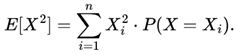
We can say that (E[X])2 is the square of the mathematical expectation calculated previously.
- 3.
- W is the total profit after N=100 intermediate blocks, given by:
- 4.
- All Xi are independent and identically
 distributed (i.i.d.), as each IB follows the same probabilistic model.
Lemma 1.
For a sequence of random variables X1, X2,..., XN i.i.d. with mathematical expectation E[X] > 0, the sample mean almost certainly converges to E[X] as N →∞
Proof of Lemma 1:
This result follows directly from the Strong Law of Large Numbers. Since E[X] > 0 by hypothesis, we conclude that:
Lemma 2.
The second lemma refers to the cumulative deviation. The cumulative sum shows a linear trend with N, where:
shows a linear trend with N, where:
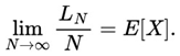
Furthermore, for any ϵ > 0:
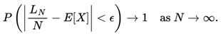
Proof of Lemma 2:
This result is also based on the Strong Law of Large Numbers. As E[X] > 0, we have:

Corollary:
If E[X] > 0, then:
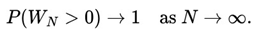
Proof of Corollary:
As  and E[X] > 0, we conclude that WN > 0 with high probability for sufficiently large N.
and E[X] > 0, we conclude that WN > 0 with high probability for sufficiently large N.3.5. Differences Between Victoria and Kelly’s Criterion
One point in common between the Kelly Criterion and the Victoria is the use of compound interest through reinvestment. However, there are some peculiarities to both approaches that we can see better in the table below.
Table 15.
Differences between Victoria and Kelly’s Criterion.
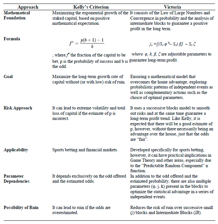
The main practical distinction is that Kelly requires the player to have an accurate estimate of the house edge in order to maximize capital growth, while Victoria can work even without such an edge, provided only that the odds are “fair”.
As we can see, Victoria reduces risk by working with intermediate blocks and small blocks, allowing better control of variability and guaranteeing a long run profitable trend only through its general formulation without considering any kind of advantage against ‘House’.
Furthermore, by design, Victoria hopes to provide potential users of the method with a robust theorization that, in addition to its positive long run mathematical expectation, will also provide more peace of mind when executing the method, minimizing the impact of psychological biases and other emotional issues that are factors that cause many bettors to lose money in this market.
3.6. Victoria and the Game Theory
3.6.1. A Brief Reflection on Some Socio-Economic Aspects and the Proposal for an Economic Model Based on Science and Statistics
Well, throughout this study, it has been a challenging task. I was expected to finish it in just over seven months. However, I have suffered a lot of pain from a deficiency of some vitamins, especially vitamin B12, which was at levels considered very serious to the point of strongly affecting my mind and nervous system. As a result, I had to postpone and complete this study by a little over ten months. I've always been overly curious and thinking about this issue, so when I went home from the medical center comfortably numb, I reflected a little on some socio-economic issues, such as:
- Could factors such as the higher the rate of the population with a satisfactory nutritional base (in terms of vitamin balance...) in the body have a positive influence on a higher quality of life, to the point of preventing and minimizing the impact of diseases? How could such a nutritional base influence the process of generating wealth for nations over the years in the medium and long term? Could these countries be more socially and economically developed than others whose populations have a lower percentage of citizens with a satisfactory nutritional base?
- Could socio-urban aspects such as countries that have higher rates of sidewalks and other organized and standardized constructions positively influence quality of life indices as well as the process of wealth generation for nations over the years in the medium and long term?
As far as the first question is concerned, Fontaine et al. (2003) carried out an in-depth study on diet as well as other hereditary factors, considering different categories such as age, ethnicity and analyzing how Body Mass Index (BMI) could also influence the metric of Years of Life Lost (YLL). Overall, the study came to the conclusion that overweight has a significant impact on quality of life, especially among younger people.
This premise raised as imagined is not new and I was very excited by the results found through the study by Wang and Taniguchi (2002) which indicate that improving nutritional status has a positive and significant impact on long-term economic growth. In particular, we can estimate that an increase of 500 kcal/day in the average supply of food energy per capita can increase the growth rate of real GDP per capita by approximately 0.5 percentage points. This effect is particularly significant in East and Southeast Asian countries, where the magnitude of the impact can be up to four times greater.
Furthermore, Wang and Taniguchi (2002) also point out that However, for other developing economies, the relationship between nutrition and growth tends to be negative or statistically insignificant in the short term, possibly due to the dynamic interactions between population growth and labor productivity. These findings suggest that policies aimed at reducing malnutrition can generate not only humanitarian benefits in terms of quality of life, but also significant gains in terms of sustainable economic growth. Ogundari and Aromolaran (2017) through their case study in sub-Saharan Africa also found significant results regarding the correlation between better levels of nutrition and an increase in a region's GDP.
With regard to this question about socio-urban aspects, it is assumed that the lack of standardization, for example, of sidewalks and streets, can mean that each citizen, whether on foot or in their vehicle, requires a little extra energy to observe, reflect and act in the face of disorganized environments with too many obstacles in front of them, whether they are commuting to work, going home, or simply going shopping.
The question that remains is what could be the impacts on both the quality of life of each citizen and the economy of a nation, a city that has high rates of disorganization of its public roads could bring over a year, 5 years, 10 years, 30 years?
What should be clear and understandable in this questioning is that these small amounts of energy demanded are nothing more than “human depreciation”. In the long term, these people could have more vitality and time to deal with other issues, whether for their own personal well- being or even with this “saved” energy, they could be in a position to contribute even more to generating wealth for their local community, whether through working more on projects for their own self-realization or developing new technologies and knowledge that could generate added value and be patentable.
During this time, people traveling on public roads in a disorderly manner can lead to higher rates of accidents and even deaths, and consequently tend to increase public spending on the health sector, which is even more sensitive for those countries that have a unified health system. Once again, the sum of these avoidable accidents over the long term could prevent new investments in other sectors.
This relationship between the socio-urban aspects theorized here is not new, but has also been addressed by other authors such as Khalil (2012), who emphasizes that Gross Domestic Product (GDP) should not be seen as the main tool for assessing a population's level of well- being. The author investigates how strategic urban planning can be a tool for increasing the quality of life perceived by citizens.
Another interesting study was by Deng et al. (2018) in which we see that urban planning has a significant effect on controlled urban growth within the Special Economic Zone (SEZ) as was observed in the case study in Shenzhen, China.
The case study observed on Chaharbagh Abbasi Street in Isfahan, Iran, by Shahmoradi et al. (2023) shows that pedestrianization can initially have negative impacts, such as the closure of 27.5% of traditional businesses and the stagnation of sales and job creation. However, in the medium and long term, it has shown promising potential for increasing economic activity, as pedestrian traffic has increased by 64% and new food and beverage outlets have increased by approximately 60%. As the authors emphasized, the results found in this region can be better analyzed in other contexts to see if this practice, considered sustainable, can promote both the health and well-being of citizens and expand the local economy.
In addition to these two questions, there is a third: could countries in which Sportsbooks have lower annual revenues than other countries (in percentage terms) somehow at the same time imply a population that is better educated about personal finance and knowledge of statistics?
Could we measure this and create new economic metrics from this point? In fact, we must also take into account that correlation does not imply causality, but it could be an invitation to analyze variables that deserve to be better investigated in detail.
Furthermore, as Banerjee and Duflo (2011) put it in their study on new economic perspectives for minimizing poverty through the understanding that as human beings interacting with the natural world we result in complex systems, perhaps we should look more at the details and particularities of each place to understand the reasons for “poverty” instead of coming up with economic models with the aim of generalizing across the globe.
Douglass et al. (2024) demonstrated how statistics can be present and impact on results in Olympic Games. Mesquita et al. (2010), using data analysis and statistical techniques, analyzed the climatic properties of extratropical storms in the North Pacific Ocean and the Bering Sea, regions known for their high cyclone activity and storm tracks. Thus, Political decisions should be focused on statistics and science rather than political ideologies which tend to lead us into a game whose payoff will be negative and/or at best a relatively slow growth in human progress. By asking these simple questions and redirecting the way we think about the natural world and our interaction with it, we can surely make relevant discoveries that could lead to a fairer world with a better quality of life for everyone.
3.6.2. Predictable Random Component Function (η(Xt))
Assumptions and definitions:
- Consider a game G with N players g1, g2, ..., gN.
- Randomness in the game follows a uniform distribution U(a,b).
- The η(Xt) (Predictable Random Component) function represents the factor that connects the player's knowledge to their ability to exploit randomness and other additional actions.
- Each player gi has a strategy si and an expected payoff [πi].
Definition of the η(Xt) function:
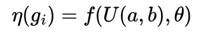
Below are some of the conditions of the problem:
- Each player gi, using his advanced knowledge of randomness and mathematical or physical operations, defines a
 strategy that ensures that in the long term his expected payoff will be positive.
 - After n sequences of moves, the strategy guarantees that [πi ] > 0, regardless of the behavior of the other players.
In formal terms,
for gi, we define η:ℝk → ℝ, where η is a function that incorporates:
- The player's knowledge of the uniform distribution U(a,b);
- Mathematical operations f(x), physical operations h(x) or any other cognitive action.
Since the objective is always to guarantee a positive value, the si strategy must satisfy the following condition:
This means that, regardless of the conditions of the game and the strategies of the other players, the application of the η(Xt) function must ensure that the cumulative sum of the returns is never negative.
For each player gi, we define a strategy si that depends exclusively on the function η(Xt):
Positive expected payoff condition: For any n∈ℕ:
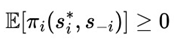
Dependence on the η function:
The si strategy depends on the η(Xt) function, i.e:
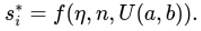
Under these conditions, player gi can guarantee a positive expected payoff in each sequence n, regardless of the opponent's strategies.
The Predictable Random Component approach redefines the player's strategy by focusing on the sustainability of returns with positive payoffs, unlike approaches such as the Kelly Criterion that seek to optimize the expected gain, the η(Xt) function (or fv(Xt) function in the context of VNAE) establishes a strategy where the rigorous application of the statistical model guarantees that E[πi] > 0 always, providing positive cumulative growth over time.
3.6.3. Victoria-Nash Asymmetric Equilibrium (VNAE)
Let a stochastic game be formalized as a tuple: G = (N, S, U, P),
where,
N = {1, 2,..., n} represents the set of players;
Si is the set of strategies available to each player i; Ui : S →  is the utility function of each player;
is the utility function of each player;
P is a probability distribution that models the randomness present in the game.
fv(Xt) = The fv(Xt) or η(Xt) function (or simply, η or fv function) refers to the fact that within a game in which the randomness factor in a uniform distribution is crucial to it, any player who has advanced knowledge of randomness added to other additional actions, whether with the support of statistics, mathematical and/or physical operations, will be able to determine an optimal strategy whose results of the expected value of the player's payoff will always be positive regardless of what happens after n sequences determined by the player.
We define a stochastic process Xt associated with the game, where the dynamics of states follows a distribution P(Xt). We assume that:
In “Predictable Random Component” there is a function  such that:
such that:
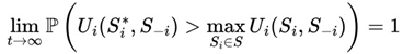
It is important to mention that in the convergence in probability of the optimal strategy there is a strategy such that:
such that:this implies that player i can maintain a continuous statistical advantage over time.
Theorem:
If there is a function fv(Xt) such that the randomness of the game shows partial predictability, then there is at least one player i with a strategy that allows continuous advantage, shifting the equilibrium to an asymmetric state.
that allows continuous advantage, shifting the equilibrium to an asymmetric state.As a way of demonstrating this, we can apply, for example, the fixed point theorem whose references to Brouwer (1911) and Banach (1922) as well as Markov processes.
First, let's approach this proposed model from the perspective of the fixed point theorem.
Let G = (N, S, π) be a stochastic game, where N represents the set of players, S1 × S2 × ... × Sn is the space of available strategies and πi : S × X → is the payoff function for each player i.
is the payoff function for each player i.It is also assumed that each player can choose a strategy si∈ Si and that Xt ~ U(a, b) represents a stochastic process with uniform distribution in the interval (a, b). A predictable function fv(Xt) is defined, representing the structurable component of randomness, so that a player's payoff function is given by:
where gi(s, Xt) is a continuous function and εt ~ U(c, d) represents random noise. We can define the best response function as B(s), which returns the optimal strategy for a player, given the strategy of the other players, as
πi (s, Xt) = gi(s, Xt) + εt
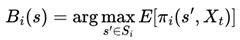
The aim is to demonstrate that there is at least one set of strategies  such that
such that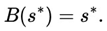
To establish this result, we use Brouwer's Fixed Point Theorem, which guarantees the existence of at least one fixed point for any continuous function defined over a convex and compact set, since it is a closed and bounded subset of n, and convex, since it allows mixed strategies.
n, and convex, since it allows mixed strategies.In addition, it should be clear and understandable that the continuity of the best response function B(s) follows from the continuity of gi(s, Xt) and the linearity of the mathematical expectation. Since B(s) is a self-mapping function in S, satisfying all the hypotheses of Brouwer's Theorem, it follows that there is at least one such that  guaranteeing the existence of an asymmetric Victoria-Nash equilibrium where a player can exploit predictable patterns of randomness in a sustainable way.
such that guaranteeing the existence of an asymmetric Victoria-Nash equilibrium where a player can exploit predictable patterns of randomness in a sustainable way.Let’s consider the dynamics of the game as a Markov process where the state Xt evolves according to:


This means that εt is a purely random term and therefore has no temporal correlations.
The maximum “predictability” has already been extracted by fv(Xt), i.e. the entire exploitable and expected pattern of true randomness has been identified. What remains (εt) is truly unpredictable, which we can say is the majority, demonstrating that the advantage exists, but there is a statistical limit to exploiting it.
By hypothesis, fv(Xt) captures part of the random structure of the game, making Xt partially predictable.
If Xt is partially predictable, then there is a strategy such that:
such that:
This means that player i can adjust his strategy according to exploitable patterns of randomness, ensuring that his expected utility is consistently higher.
We can define the new equilibrium as a state where:
a state where: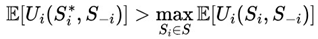
this means that player i maintains a long-term advantage, even if the other players optimize their strategies.
Since this advantage cannot be neutralized by the other players, the game converges to an asymmetric state in which player i sustains a continuous strategic edge. This result deviates from the classical Nash Equilibrium, which assumes that no individual player can maintain a persistent advantage and that all participants operate under conditions of strategic parity.
As we can see, the VNAE has some implications for Imperfect Information Games, since it modifies the conception of imperfect information games by suggesting that randomness can be partially predictable for certain strategic agents.
Let G′ be an imperfect information game, where each player i has subjective beliefs πi(h) about the historic h of the game. Traditionally, these beliefs follow the Bayesian updating rule:
However, if P is structurally partially predictable under fV(Xt), then classical Bayesian updating can be replaced by a 'deterministically adjusted' version, where certain events can be anticipated and/or expected in the long term due to factors such as convergences in probabilities, for example. This changes the expected strategic behavior in financial markets, betting and other decision games in different areas in which the randomness factor is an important basis for the system.
Although it still maintains the basic essence of the Nash Equilibrium, in VNAE the idea of a “fair” and symmetrical equilibrium as we can see no longer exists, because exploitable predictability alters the structure of the game in which one of the players tries to respond by minimizing their disadvantage.
Despite its asymmetrical nature, it is also important to think about two possible scenarios:
- I.
- the central idea of the VNAE in which one side will always have a structural advantage through the fv function, thus leading to an inevitable and immutable asymmetric state and;
- II.
- the response of the players at a disadvantage being able to adopt a minimization strategy and, depending on this, reach a new equilibrium and/or advantage for one of the sides at another point.
In fact, the Victoria methodology redefines the structure of strategic equilibrium by demonstrating that randomness can be exploited for sustainable advantages within stochastic games. The Victoria-Nash Asymmetric Equilibrium proposes an extension of game theory by integrating statistical predictability into games with uncertainty, as opposed to the idea that optimal strategies always converge to stationary states of no advantage.
In the framework of the Victoria-Nash Asymmetric Equilibrium (VNAE), despite the presence of structural asymmetry, a given player can sustain a long-term strategic advantage
without the possibility of complete neutralization by opposing agents. Its equilibrium consists of its transformation into a new state, in which statistical predictability - combined with additional physical and/or cognitive strategic adjustments (such as advanced knowledge of randomness in a uniform distribution and some mathematical and/or physical operations, for example) - fundamentally alters the underlying dynamics of the game.
Victoria through the fv(Xt) function by allowing sustained advantage, then the dynamics of the game change to a state where that player becomes dominant. However, this dominance, as stated above, may not be absolute, since there may be scenarios in which the other participants or external factors may adopt strategies (for the purpose or not) of mitigation, creating (again) a new equilibrium structure and even changing the rules of the game which, in this case, would not only modify Victoria-Nash but also the Nash equilibrium itself in its essence.
The idea presented here is just a simple start for something that needs to be further developed, especially considering practical applications in various other areas of science, from information security to artificial intelligence and biology, for example.
3.6.4. Victoria-Nash Asymmetric Equilibrium (VNAE) in a Nutshell
Let there be a stochastic game G with N rational players, where each player i chooses a strategy si ∈ Si to maximize his expected payoff. In this model, we consider the existence of a predictable random component fv(Xt) within the randomness allowing a player to explore statistical patterns given a uniform distribution and employ complementary actions such as using mathematical operations, physics and/or any other cognitive actions.
Formally, a set of strategies  constitutes a Victoria-Nash equilibrium (VNAE)
constitutes a Victoria-Nash equilibrium (VNAE)if, for each player i, there is a predictable random component fv(Xt) such that its optimal strategy
maximizes the expected payoff conditional on this predictable structure of randomness. Below is its formulation:

Ui() : player i's expected payoff when choosing the strategy .
) : player i's expected payoff when choosing the strategy .
Pi(si, s-i) : Traditional payoff function, based on the interaction between the players' strategies.
fv(Xt) : predictable component within the randomness of the game, allowing statistical patterns to be identified.
 : set of information available to player i at the time of the decision, which influences his/her strategic choice.
This formulation implies that, in a Victoria-Nash Asymmetric Equilibrium, certain players can gain sustainable long-term advantages by identifying predictable patterns within the randomness of the game, which leads them to an asymmetric equilibrium.
As we can see, if fv(Xt) is relatively small or zero, the VNAE can converge to a Nash Equilibrium.
Impacts can be expected in stochastic games, zero-sum games, asymmetric games, repeated games, imperfect information games as well as an extension of Nash Equilibrium and Bayesian Equilibrium, for example.
3.6.5. Victoria-Nash Asymmetric Equilibrium General Applications
As we saw earlier, there is a function fv(Xt) that allows us to extract and partially predict the randomness in a stochastic game, specifically, considering a uniform distribution. In summary, what should be clear and intelligible is that through the function η(Xt) (or fv(Xt) in the context of the Victoria-Nash Asymmetric Equilibrium):
- the model expands the classic concept of equilibrium by incorporating partial predictability of randomness as an integral part of strategy,
- this scenario leads to one player managing to maintain a sustained strategic advantage over the long term,
- this advantage leads us to an asymmetric state in which one side has a structural advantage after applying a dominant strategy through the fv(Xt) function (Predictable Random Component),
- It modifies the structure of zero-sum games and imperfect information games, creating new forms of strategic equilibrium.
- however, there is the possibility of other players trying to mitigate this advantage as well as leading to a possible new equilibrium and/or an advantage for one side at another given point.
The model departs from the classic Nash Equilibrium, as it allows for a structurally asymmetrical and potentially dynamic state. Even though it is an asymmetric equilibrium, players rationally continue to maximize their strategies within the game, maintaining the basis of the central principle of the Nash Equilibrium.
The η(Xt) function as well as the Victoria-Nash Asymmetric Equilibrium can have practical applications in the biological sciences and ecology through a variety of studies, from modeling bacterial cultures, tumors, to analyzing behavior patterns in animals (based on 'instinctive rationality' through biological reinforcements and survival through natural selection) in which the randomness factor and uniform distribution can be present as a basis for study.
Following the same reasoning, the identification of lottery designs in which there can be positive mathematical expectation for the player. Although the author didn't go into it in depth, I have noticed this issue and the real possibility that some lotteries around the world (especially those whose designs lead to more accessible jackpot odds for a player with a single ticket to win)
- may be theoretically 'vulnerable' to victorian players employing convergence in odds as a decision-making tool, as other colleagues have also presented similar results over time, as in the case of Stefan Mandel and, more recently, by Stewart and Cushing (2023). The same thought applies to other random games such as roulette: probably the only way for a player to be a winner using statistics (and not relying on physical deviations of the roulette wheel and/or PRNG algorithms used in digital roulettes) is to deeply understand the convergences in probabilities added to other complementary actions, as well as counting on the monetary values per bet and returns also being favorable to him.
In the groundbreaking work "Mick Gets Some (The Odds Are on His Side) (Satisfiability)" by Chvátal and Reed (1992), the authors explore probabilistic properties of random Boolean formulas within the k-SAT framework, establishing critical thresholds for satisfiability and demonstrating the probabilistic dynamics underlying solution spaces. By leveraging advanced algorithms such as Unit Clause (UC), Generalized Unit Clause (GUC), and Shortest Clause (SC), the study reveals how structural randomness in clause-variable relationships can lead to high-probability satisfiability outcomes under specific configurations.
As we can see through Chvátal and Reed (1992), the probabilistic approach to satisfiability resonates with the principles underlying Victoria-Nash Equilibrium, particularly in its focus on exploring predictable patterns in stochastic environments. In this sense, we can expect contributions from VNAE to future studies in the area of computing and optimization in this direction.
In addition to the aforementioned environments, it is also hoped that, based on the same principle of the η(Xt) function, applications in the field of cryptography may also be possible, to a certain extent, especially in terms of trying to reduce the number of possible combinations in randomization algorithms, which this study can provide as an additional focus for professionals in this field.
In economic systems, especially in financial markets, the existence of the Victoria-Nash Asymmetric Equilibrium may be present in possible applications of hedge funds considering different types of investment markets.
Considering that one of the fundamental bases in areas such as data science and artificial intelligence is the identification of patterns that can result in a descriptive or predictive model, as we can see in the recent paper by Martins and Papa (2023) in which they present a new clustering approach based on the Optimum-Path Forest (OPF) algorithm. In this sense, we can also expect that Victoria and its respective ‘equilibrium’ could provide new perspectives for this field, helping to identify patterns and make decisions.
Furthermore, through the field of study of Neutrosophic Statistics formalized by Smarandache (1999) and Smarandache (2014) as an extension of Classical Statistics that incorporates the indeterminacy factor (I) in probabilistic models, it is also believed that Victoria could also have applications in this sense and, adapting to this emerging field, the predictable random component can be defined as:

“Truth” p(T), ‘Indeterminancy’ p(I), and ‘Falsity’ p(F) represent the neutrosophic components of an uncertainty distribution in a strategic game;
ξ represents an uncertain but partially modelable component and ε represents pure random error.
There is also a positive expectation for practical applications within the field of physics studies, especially in dynamical systems where they have strong approaches to finding patterns in chaotic systems. Furthermore, Victoria-Nash Asymmetric Equilibrium in several other subfields - from meteorology, plasma physics and nuclear fusion control to quantum mechanics and non-linear optics - can help exploit asymmetric advantages and optimize complex systems. It is therefore believed that it can open up new avenues for control, efficiency and innovation in various fields of physics.
Mathematical modeling as well as randomization is very present in studies in the field of biological sciences and ecology, as can be seen from Johnston et al. (2007) when applying mathematical models to model colorectal tumors, for example. As we can see from the study presented by French et al. (2012), in randomised clinical trials the allocation of patients between treatment and control groups is designed to be completely random in order to reduce bias while ensuring statistical validity. However, the VNAE suggests that, even in this context, there may be predictable structures in the response to treatment, which can be explored mathematically.
Convergence in probability tells us that as the number of observations increases, the sample means of a specific subgroup get closer to an expected value. In this way, even in an environment where randomness dominates allocation, certain patients may show predictable patterns in their response to treatment, making it possible to anticipate the behaviour of certain subgroups.
Let Yi be the response to treatment of patient i. We can model this response using the following formulation:
μ : represents the expected mean response to treatment;
ηi : represents a predictable random component within the randomness of the group to which the patient belongs;
εi : represents the random error or ‘random noise’ (the part of the randomness that cannot be tamed)
If convergence in probability is valid, then for a specific subgroup G, we have:
In addition, identifying these predictable patterns can help correct structural biases in randomization. In fact, certain factors such as genetic factors, age and previous medical conditions can influence the response to treatment in a systematic way, creating a bias that can compromise statistical inference. In any case, VNAE can make it possible to model these structural variations, improving the interpretation of results and optimizing decision-making in clinical trials.
The approach proposed in this study may make it possible to adjust statistical analyses to take into account the predictability that exists within randomness, ensuring that conclusions about, for example, the effectiveness of treatment are more robust and representative of reality. Here, instead of using the function fv(Xt) with the aim of the gambler generating consistent profits against other gamblers as well as against the ‘house’, we simply convert it into the mathematical-medical language in which health professionals will ensure that patients obtain additional asymmetrical advantages in dealing with their respective illnesses.
As we can see, this is still a new study and therefore new perspectives for practical applications will emerge over time. In this sense, the entire academic community is invited to discuss and delve deeper into this theorization of Victoria in their respective areas of expertise, especially those in which I do not have relevant knowledge such as physics and biological sciences and that I am unable to draw any assertive conclusions in this regard and that these colleagues will surely do a better study than me.
3.6.6. Social Science Applications of the Asymmetric Victoria-Nash Equilibrium
The presence of randomness in social games can be modeled by a uniform distribution Xt
~U(a, b), representing the uncertainty inherent in human existence and human interactions, such as variations in individual preferences, access to resources and opportunities and the impact of unpredictable external factors. Nevertheless, within this randomness, certain rational agents can exploit predictable patterns, gaining a sustained strategic advantage over time.
The Victoria-Nash Asymmetric Equilibrium (VNAE) describes this asymmetry by incorporating a predictable component fv(Xt) within the stochastic structure of the game, allowing individuals or groups to maintain continuous influence even in environments subject to random fluctuations. This is because, although social decisions have a degree of uncertainty, certain structural attributes - such as economic capital, networks of influence, dominance over communication channels - create a systematic bias that favors agents with a greater capacity for foresight and strategic adaptation.
In this context, elements known as natural gifts, charisma, talent, long periods of training, and structural inequalities act as factors that allow partially predictable patterns to be identified and exploited in social interactions. Individuals with superior communication skills, for example, can 'predict' and influence group behavior, consolidating leadership positions in social networks and negotiation practices. Similarly, in the global economy, nations with industrial and technological superiority have predictable advantages over emerging countries, being able to anticipate strategic positions and reactions and adjust their policies to maximize gains, even in the face of external uncertainties.
As we can see, when applied to social science contexts ranging from psychology and sociology to interpersonal relations and geopolitics, the concept of predictable patterns of randomness consists of the sum of natural advantages (or a person's natural gifts and talents) and structural advantages (in terms of resources and access to opportunities), as well as the ability to identify environmental and social patterns to increase their payoff.
In sociology, for example, sensitive topics such as access to education can become an example of how certain social groups with greater access to information and 'elite education' undeniably tend to have an asymmetrical advantage over other players in the same game. Even if a student from a 'poor education system' comes to be at the same level as others over a period of time, those belonging to the elite education group can still remain with a constant structural advantage over time.
In the social environment, the impression we may have that the positive results of something don't matter, but rather who presents them, can be modelled and explained by a mathematical model that shows asymmetrical advantages for one side.
When analyzing social inequality from the perspective of game theory, it becomes even more necessary to debate how public policy can offer equal opportunities to all rational agents in this game called real life. Other sensitive topics, such as income distribution, the problem of hunger and nutrition, access to health care, among others, also follow this same line of reasoning in which certain individuals tend to have asymmetrical advantages over others even if they are in the same position and carrying out the same activity.
Thus, briefly, VNAE provides a mathematical model to explain how strategic agents can use structural characteristics to transform a stochastic environment into a predictable dynamic, sustaining long-term asymmetric advantages as well as shaping strategic equilibria, including in complex social systems.
3.6.6.1. VNAE Applied to the Battle of the Sexes
Just like the classic version of the game, let's consider that a couple wants to decide between going to two events: Opera (ρ) and Football (τ). The woman prefers to go to the opera, while the man prefers soccer, but they both value being together more than going alone to the event of their choice.
Traditionally, the game features two pure Nash equilibria (ρ, ρ) and (τ, τ) and a mixed equilibrium where players can randomize their choices. However, with the introduction of VNAE, we consider that the woman has a predictable advantage factor fv(Xt), which is interpreted as a social bias, a historical decision pattern and/or a psychological inclination, for example, which means that even when faced with apparently equal decision scenarios, the woman may still have some tendency, a slight advantage in her favor.
In this sense, as a slightly exaggerated hypothetical example, we can also infer that if fv(Xt) is large enough, the equilibrium in which the woman manages to go to the opera becomes the only sustainable one in the long term, characterizing an Victoria-Nash asymmetric equilibrium in which one player maintains a continued strategic advantage by exploiting predictable patterns in social interactions.
3.6.6.2. VNAE Applied to Geopolitical Scenarios
Let's consider a strategic game between Nation A and Nation B in which both compete for geopolitical influence. It is known that Nation A has structural advantages such as greater industrialization, development of new technologies, global media influence, military dominance and dominance over international institutions, for example. On the other hand, Nation B, despite also being competitive in the open-market, has fewer resources but still tries to maximize its interests. Both can opt for two main strategies Cooperation (C) or Conflict (W).
When we consider the effect of Nation A's superior industrialization, global media influence and military power, we can see that it generates a predictable structural advantage in any conflict scenario with Nation B. This factor is represented by the Predictable Random Component fv(Xt), which increases Nation A's payoffs whenever there is competition or confrontation. Below is a table containing the payoff matrix according to the VNAE:
Table 16.
Payoff matrix between two nations according to the Victoria-Nash Asymmetric Equilibrium.
| Nation B: C | Nation B: W | |
|---|---|---|
| Nation A: C | (3, 3) | (1, 4) |
| Nation A: W | (4 + fv(Xt), 1) | (2 + fv(Xt), 2) |
We can conclude that whenever Nation A opts for W (conflict), its payoff is increased by fv(Xt), as its structural superiority ensures that it loses less and gains more in rivalry scenarios. Consequently, this alters the balance of the game, making the equilibrium asymmetrical and favoring more aggressive strategies on the part of Nation A, which can sustain a dominant stance without suffering proportional losses.
Furthermore, for Nation B, this leads to a lock-in effect, where cooperation (C, C) becomes the only sustainable option in the long term, since any attempt to challenge Nation A's hegemony could lead to disproportionate results. In this way, in the field of international relations, the VNAE can explain how a dominant power can maintain a strong influence on the geopolitical scene even in the face of uncertainty and explicit rivalry.
3.6.7. Differences Between Victoria-Nash Asymmetric Equilibrium (VNAE) and Stackelberg Equilibrium
The discussion in the previous section about possible applications of the VNAE within the field of social sciences inevitably leads us to ask about the main differences between the equilibrium proposed in this study and the well-established one called the Stackelberg Equilibrium, above all due to the fact that both deal with asymmetry within a game.
Below, through Table 17, we will see some of the main differences between the two theories:
Table 17.
Differences between Victoria-Nash Asymmetric Equilibrium (VNAE) and Stackelberg Equilibrium.
Table 17.
Differences between Victoria-Nash Asymmetric Equilibrium (VNAE) and Stackelberg Equilibrium.
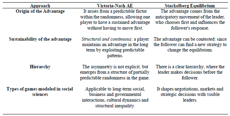
As we can see from Table 17, both have asymmetry as a central focus and one of the players has an advantage over the other, but with different approaches to the origin of the advantage and hierarchy, for example. Next, we'll look at some of the expected practical applications for VNAE and those that usually occur with Stackelberg Equilibrium within the field of social sciences:
Table 18.
Some real-life applications of Victoria-Nash Asymmetric Equilibrium and Stackelberg Equilibrium.
Table 18.
Some real-life applications of Victoria-Nash Asymmetric Equilibrium and Stackelberg Equilibrium.
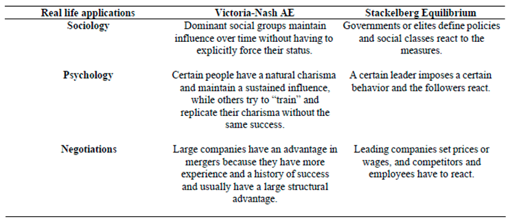
3.6.8. Differences Between Victoria-Nash Asymmetric Equilibrium (VNAE) and Bayesian Equilibrium
The Victoria-Nash Asymmetric Equilibrium (VNAE) and the Bayesian Equilibrium differ fundamentally in the way they treat uncertainty and the strategic structure of the players. In Bayesian Equilibrium, agents make rational decisions based on subjective beliefs about the state of the game and the types of opponents, updating these beliefs as new information is observed, using the Bayesian update rule. This equilibrium assumes that, as the game evolves, players adjust their strategies until none of them can unilaterally improve their expected outcome, leading to a state of informationally efficient equilibrium.
In contrast, VNAE proposes that, in stochastic games, part of the randomness may contain structurable patterns that, added to other additional actions such as mathematical or physical operations as well as any other ‘cognitive’ action, an agent can exploit systematically. This implies that a player can maintain a sustained strategic advantage over time, creating an asymmetric equilibrium, where at first, given scenario I, the optimization of opponents is not enough to completely neutralize this advantage.
While Bayesian equilibrium assumes that uncertainty is inherent and ineliminable, VNAE suggests that certain agents can structurally reduce uncertainty, shifting the equilibrium to a state that is persistently favorable to a specific player. Thus, we can begin to see the existence of purely Bayesian players and purely victorian players (those who use the function η(Xt) in their decision-making).
The concept behind the Predictable Random Component function, given the experience I have had in the course of this study as well as drawing on the vast literature of colleagues over time, does not seem absurd to me, but increasingly clear and intelligible as well as realistic within the context of Decision Theory and Game Theory.
As can be seen in the section “Is it Possible to Beat the House?” many scientists and people driven by curiosity in the field of mathematics and statistics have exploited patterns normally expected by the law of large numbers and other types of convergence in probability to beat the house. In fact, in this very study, through the Victoria formula, the PRC (Predictable Random Component) proved to be a more strongly applicable example for positive mathematical expectation and systematic financial gains in the long run.
In the case of this study, through Victoria, we note that the predictable random component (PRC) is understood as convergence in probability, however, with the eventual advances in scientific and statistical thinking as well as new disruptive technologies such as those coming from quantum mechanics, paradoxically, they can also lead us to deepen and better understand the true nature of randomness given a probability distribution and why certain numbers/events occur in t period of time and n place. As Poincaré (1908) and many other colleagues throughout history have pointed out, as human beings we consider as random everything in which we are unaware and/or which cannot be fully quantified. But this scenario could be better explored, especially with new generations of academics.
In fact, we can observe a connection between the optimal strategy and the η(Xt) function in which we could perhaps also classify it as simply part of the optimal strategy found by a player. However, since we are taking as examples the very nature of randomness given a probability distribution, in the case of this study the uniform distribution has been used, something inherently immutable, perhaps we should propose a reflection in the sense of extending η(Xt) or fv(Xt) as a basic function in relation to the others that normally constitute a basic game in this field of study. Below, with the table x, we will see more differences between these two theorizations.
Table 19.
Differences between Asymmetric Victoria-Nash Equilibrium and Bayesian Equilibrium.
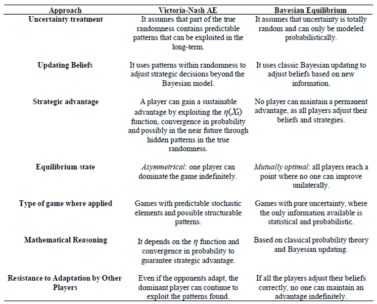
3.6.9. Differences Between Victoria-Nash Asymmetric Equilibrium and Nash Equilibrium
In this part of the study, we will analyze some fundamental differences between the Victoria-Nash Asymmetric Equilibrium and Nash Equilibrium Differences, considering different approaches from their definition to the critical point of these theorizations.
Table 20.
Differences between Asymmetric Victoria-Nash Equilibrium and Nash Equilibrium.
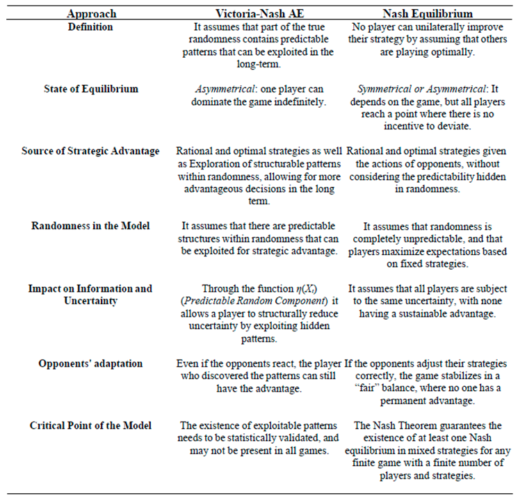
Below, also for better visualization purposes, a table is also used to demonstrate some examples of possible real-life situations involving these two types of equilibrium.
Table 21.
Differences between Asymmetric Victoria-Nash Equilibrium and Nash Equilibrium with real life applications examples.
Table 21.
Differences between Asymmetric Victoria-Nash Equilibrium and Nash Equilibrium with real life applications examples.
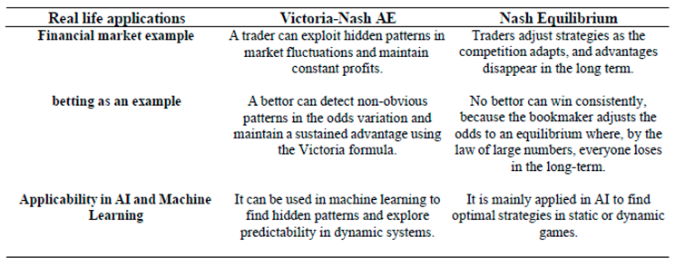
As we can see from the tables in this section, the Victoria-Nash Asymmetrical Equilibrium (VNAE) differs from the Nash Equilibrium by allowing a player to sustain a continuous strategic advantage by exploiting predictable patterns (i.e. convergences in probabilities) within the randomness of the game.
While the Nash Equilibrium assumes that all players adopt optimal strategies, leading to a point where no one can unilaterally improve their position, the VNAE suggests that certain players can find predictable structures in uncertainty, which allows them to make more advantageous decisions in the long run. This ability to exploit hidden regularities makes the equilibrium asymmetrical, since one agent can maintain a dominant position even if the others adjust (according to scenario I).
Unlike the traditional Nash model, which assumes a static scenario where strategies converge to a point of mutual equilibrium, the VNAE proposes a dynamic equilibrium, where a player can continue to make structural gains due to the continuous exploitation of patterns in true randomness and/or with actions not completely mitigated by the other players. This challenges the idea that, in the long term, all competitive advantages disappear as players adjust their strategies.
If Sportsbooks were to adopt extreme restrictions such as limiting the amounts wagered, limiting bets on certain sports markets and even banning victorian players, the VNAE equilibrium would still remain unchanged, since Sportsbooks are not only adjusting their strategies within the game, but changing the external rules of the market, which also does not characterize a Nash Equilibrium, since the original game is modified to prevent certain players from fully participating.
Thus, VNAE redefines the notion of equilibrium in Game Theory by including the possibility of persistent advantages for certain players, which has direct implications for financial markets, cybersecurity, biological sciences, artificial intelligence and risk modeling in sports betting, for example.
3.6.10. Sportsbooks' Possible Defensive Reactions to the Victorian Players
As has been seen throughout this study, in the exchange version, regardless of which players win or lose, the house always takes its share of the profit. However, in a scenario where players against the house are considered to be relatively significant in the market, sportsbooks can probably resort to some defensive measures, such as:
- Changing the way the odds are calculated by applying a higher vigorish to compensate for any losses;
- Offer less favorable odds than they normally do;
- Limiting or banning accounts that use advanced statistical strategies.
- Implementing new machine learning systems to detect victorian betting patterns.
As we can see, there are indeed some possibilities for sportsbooks to minimize this scenario of an asymmetrical advantage for certain groups of bettors. However, they will probably have to carry out a rigorous study to assess the costs and benefits of adopting measures such as increasing the vigorish as well as offering odds that are less realistic than those that could occur in sporting events. As Bontis (1996) points out and Isnard (2021) corroborates, organizations, in this case sportsbooks, need not only to have large volumes of data, but also good knowledge management, intellectual capital and available technology.
This defensive practice, if overdone, can make the task of “retaining” customers even more difficult, as well as attracting more when you have odds that may reflect reality very poorly and/or when you have a popularized slogan that the bookmaker bans bettors from certain markets or even from the platform. Such measures can discourage current customers as well as driving away potential new ones. The question that remains is to deliberately seek a point of equilibrium in which the bookmaker can still maintain its activities and, at the same time, not make players feel that they have been “probabilistically robbed”.
Sportsbooks, on the other hand, in order to expand into other territories and regulate the market, could delve into the internationalization processes of firms that address the importance of relationship and knowledge management processes, in addition to knowledge of the market itself, as pointed out by Barbosa et al (2014). Furthermore, Sportbooks may be arguing that statistics can also beat them, as presented in the literature discussed above, as well as in this study.
4. Results and Discussions
4.1. While Our Dice Gently Weeps
Well, it took a little over ten months from the development of Victoria's theorizing and practical application to the publication of this paper. So, during all that time, I’ve got a one track mind and I can say I was on a diet of tables and dice.
Due to its recency, the author, despite having carried out more than 3 million calculations manually, did not focus on making much progress in the search for the parameters φ, k and j considered "singularity point", that is, whose final results will always be positive, indicating profits 100% of the time within the 100 FVs (Future Values), but on raising the possibility, first of all, of which sets of parameters φ, k and j in this study presented (see Table 10) could at least fall into the categories of presenting probabilistically assured profitability at least 80%, 85%, 90% and 95% of the time within a sequence of 100 Fvs.
As a way of demonstrating this theorizing, we will analyse two different configurations, the first containing the following φ = 1.02; j = 2, and k = 50. In the second configuration we will analyze the φ = 1.04; j = 3, and k = 33.
The following is a reminder of Victoria's formulation:
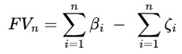 where,
IB =[(S0 φ k– S0) βi] – S0 ζi
φ = odd / probability of success of the event k = Time Period
S0 = Initial Value (fixed value used for each independent event)
βi = "Success" blocks. That is, the cost/benefit ratio compared to the investment in each stake in each n game is positive and there is some profit.
ζi = "Failure" blocks. That is, the cost/benefit ratio compared to the investment in each stake iin each n game is negative and there is some loss.
4.1.1. Analysis of the Results for the Configuration φ = 1.02; j = 2 and k = 50
We will begin by analyzing the first configuration and, in order to better visualize the results, we have considered a sequence of tables that continue a sequence of Intermediate Blocks (IB) that theoretically make up a complete Future Value (FV).
As we can see in the supplementary material, in FV96 we have 100 intermediate blocks (IB), each with 2 Small Blocks (jn), each with 50 independent events (k), which results in 100 independent events “available to play” in each intermediate block (IB). Throughout this study, random numbers between 1 and 10,000 were drawn from sources such as Random.Org, GIGACalcultator and ANU QRNG, in order to ensure reliability in the results as well as eliminate possible biases and conflicts of interest, since the author of this study has also developed a PRNG algorithm. Furthermore, in order to provide better graphic visualization of this study, the stats.blue platform was considered, as well as standard data visualization using the R language.
We can classify a Small Block (jn) as successful (β) if in the sequence of 50 numbers generated (understood as 50 independent events occurring) all the numbers are equal to or greater than 197. Similarly, if there are numbers equal to or less than 196 in the middle of the sequence, we say that we have a Small Failure Block (ζi), meaning that a bettor has lost a bet along the way.
When we put it into the formula, we get -$20, $6.92, and $33.83 as the final net results corresponding to 0, 1 and 2 Small Success Blocks (β), respectively.
It can be seen from Table 22, Table 23, Table 24 and Table 25 and Figure 21 that there are periods of volatility, however, there is a trend of continuous growth indicating positive results in the long term, although in each Intermediate Block (IB) in which, according to a standard configuration, we would theoretically expect 'only' n =100 games bet, in practice we can expect this and other potential configurations to convert between 48 and 70 games (or k independent events). With this configuration with φ = 1.02; j = 2 and k = 50, for example, we can expect an oscillation up or down of an average of 6,500 games for each FV.
Table 22.
Analysis of the FV96 with the parameters φ = 1.02; j = 2 and k = 50 Part I.
| FV96 | 0/2 | $0.00 | β / ζ |
|---|---|---|---|
| IB1 | 1 | $6.92 | β |
| IB2 | 1 | $6.92 | β |
| IB3 | 1 | $6.92 | β |
| IB4 | 1 | $6.92 | β |
| IB5 | 1 | $6.92 | β |
| IB6 | 0 | -$20.00 | ζ |
| IB7 | 2 | $33.83 | β |
| IB8 | 0 | -$20.00 | ζ |
| IB9 | 1 | $6.92 | β |
| IB10 | 1 | $6.92 | β |
| IB11 | 1 | $6.92 | β |
| IB12 | 1 | $6.92 | β |
| IB13 | 0 | -$20.00 | ζ |
| IB14 | 0 | -$20.00 | ζ |
| IB15 | 1 | $6.92 | β |
| IB16 | 1 | $6.92 | β |
| IB17 | 0 | -$20.00 | ζ |
| IB18 | 0 | -$20.00 | ζ |
| IB19 | 1 | $6.92 | β |
| IB20 | 1 | $6.92 | β |
| IB21 | 1 | $6.92 | β |
| IB22 | 1 | $6.92 | β |
| IB23 | 1 | $6.92 | β |
| IB24 | 1 | $6.92 | β |
| IB25 | 1 | $6.92 | β |
| Σ | $38.39 |
In the first 25 Intermediate Blocks, we noticed a modest positive result of $38.39, which is explained by the natural fluctuations in this market involving true randomness. This phenomenon of volatility tending towards an unimpressive profit and/or negative result can occur one or more times at any point from the beginning of the Intermediate Blocks, halfway through and at the end of each Future Value (FV). Drawing an analogy with aviation field, we can consider these scenarios as periods of “positive turbulence”, that is, despite the inconstancies in the series there is a tendency for the result to remain positive.
Table 23 shows a very satisfactory result for another group of 25 Intermediate Blocks. We can call this phenomenon of consistently positive sequences a “safe flight”.
Table 23.
Analysis of the FV96 with the parameters φ = 1.02; j = 2 and k = 50 Part II.
| FV96 | 0/2 | $0.00 | β / ζ |
|---|---|---|---|
| IB26 | 1 | $6.92 | β |
| IB27 | 1 | $6.92 | β |
| IB28 | 0 | -$20.00 | ζ |
| IB29 | 1 | $6.92 | β |
| IB30 | 0 | -$20.00 | ζ |
| IB31 | 1 | $6.92 | β |
| IB32 | 0 | -$20.00 | ζ |
| IB33 | 2 | $33.83 | β |
| IB34 | 0 | -$20.00 | ζ |
| IB35 | 1 | $6.92 | β |
| IB36 | 2 | $33.83 | β |
| IB37 | 2 | $33.83 | β |
| IB38 | 1 | $6.92 | β |
| IB39 | 2 | $33.83 | β |
| IB40 | 1 | $6.92 | β |
| IB41 | 0 | -$20.00 | ζ |
| IB42 | 2 | $33.83 | β |
| IB43 | 1 | $6.92 | β |
| IB44 | 1 | $6.92 | β |
| IB45 | 1 | $6.92 | β |
| IB46 | 1 | $6.92 | β |
| IB47 | 1 | $6.92 | β |
| IB48 | 0 | -$20.00 | ζ |
| IB49 | 1 | $6.92 | β |
| IB50 | 1 | $6.92 | β |
| Σ | $146.03 |
Table 24 shows a negative result of $69.29 for this group of Intermediate Blocks. As mentioned above, this is a natural and normal occurrence when dealing with random phenomena.
Table 24.
Analysis of the FV96 with the parameters φ = 1.02; j = 2 and k = 50 Part III.
| FV96 | 0/2 | P/L | β / ζ |
|---|---|---|---|
| IB51 | 1 | $6.92 | β |
| IB52 | 1 | $6.92 | β |
| IB53 | 1 | $6.92 | β |
| IB54 | 1 | $6.92 | β |
| IB55 | 1 | $6.92 | β |
| IB56 | 1 | $6.92 | β |
| IB57 | 0 | -$20.00 | ζ |
| IB58 | 0 | -$20.00 | ζ |
| IB59 | 0 | -$20.00 | ζ |
| IB60 | 0 | -$20.00 | ζ |
| IB61 | 1 | $6.92 | β |
| IB62 | 2 | $33.83 | β |
| IB63 | 0 | -$20.00 | ζ |
| IB64 | 1 | $6.92 | β |
| IB65 | 0 | -$20.00 | ζ |
| IB66 | 1 | $6.92 | β |
| IB67 | 1 | $6.92 | β |
| IB68 | 1 | $6.92 | β |
| IB69 | 1 | $6.92 | β |
| IB70 | 1 | $6.92 | β |
| IB71 | 0 | -$20.00 | ζ |
| IB72 | 0 | -$20.00 | ζ |
| IB73 | 1 | $6.92 | β |
| IB74 | 0 | -$20.00 | ζ |
| IB75 | 0 | -$20.00 | ζ |
| Σ | -$69.29 |
In scenarios similar to these, we can classify them as “altitude loss” flights, showing a tendency for negative results in certain parts of the journey.
Again, Table 25 shows a negative result for another group of 25 IBs, this time of $15.48, which we can classify as a period of “negative turbulence”, that is, periods of instability in the historical series indicating a slightly negative result, usually oscillating close to zero.
Table 25.
Analysis of the FV96 with the parameters φ = 1.02; j = 2 and k = 50 Part IV.
| FV96 | 0/2 | P/L | β / ζ |
|---|---|---|---|
| IB76 | 0 | -$20.00 | ζ |
| IB77 | 1 | $6.92 | β |
| IB78 | 2 | $33.83 | β |
| IB79 | 1 | $6.92 | β |
| IB80 | 1 | $6.92 | β |
| IB81 | 0 | -$20.00 | ζ |
| IB82 | 1 | $6.92 | β |
| IB83 | 1 | $6.92 | β |
| IB84 | 2 | $33.83 | β |
| IB85 | 0 | -$20.00 | ζ |
| IB86 | 0 | -$20.00 | ζ |
| IB87 | 1 | $6.92 | β |
| IB88 | 1 | $6.92 | β |
| IB89 | 2 | $33.83 | β |
| IB90 | 0 | -$20.00 | ζ |
| IB91 | 0 | -$20.00 | ζ |
| IB92 | 0 | -$20.00 | ζ |
| IB93 | 1 | $6.92 | β |
| IB94 | 1 | $6.92 | β |
| IB95 | 1 | $6.92 | β |
| IB96 | 0 | -$20.00 | ζ |
| IB97 | 0 | -$20.00 | ζ |
| IB98 | 0 | -$20.00 | ζ |
| IB99 | 2 | $33.83 | β |
| IB100 | 0 | -$20.00 | ζ |
| Σ | -$15.48 |
As we can see from both the tables and Figure 21, despite all the oscillations along the way, we had a positive result of $99.65, indicating a profit over a Future Value (FV). The results of the FV96 simulation can be accessed through the supplementary material in this study.
Since we are dealing with true randomness and convergences in probability, the popular expression “what goes around, comes around” becomes valid in this context, since if certain numbers belonging to positive results have come out it is (usually more than expected) likely that at certain times throughout each Small Block (jn) or in several Intermediate Blocks there will also be a sequence of values with 'neutral' and negative results. As we can see, this behavior, governed by the orchestra of the law of large numbers, balances the scales at some point to ensure that the final results converge on certain expected points given an expected range and its respective margin of error. Despite its controversial relationship with parts of the gambler's fallacy, ignoring this fact is like saying that a bird doesn't have wings and/or a lion is vegetarian by nature.
As will be discussed further below, we will see that this result was a poor one compared to other various FV scenarios. However, since - the objective in Victoria is not to maximize profits but to guarantee a mathematical formulation that always tends to present a positive result in the long run - we can say that the mission was well completed. If we assume that a bettor called Bob played 5700 games throughout this series of Small Blocks, Intermediate Blocks (IBs) to complete a FV, we can say that each bet resulted in approximately $0.0175 cents considering that each stake was $10.
Figure 21.
Graphical analysis of profit or loss of FV96 with parameters φ = 1.02; j = 2 and k = 50.
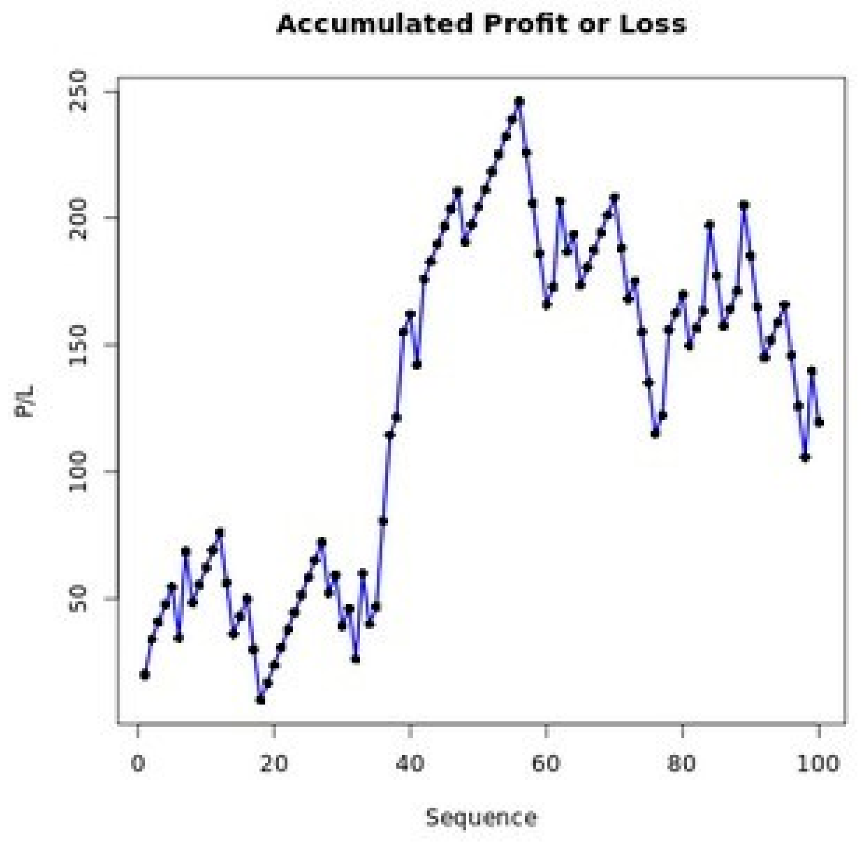
As we can see from the following tables, when we simulated 100 FVs we had 98 with positive results and only 2 with negative results (FV38 and FV62), which gave us a final positive result of $32,503.02. In fact, along this long trajectory we also had other significant results which we could consider a warning sign. This signal, which we can call the “Yellow Zone”, could come from those FVs containing a negligible profit approaching zero and tending in a negative direction. In this case, the user is advised to consider some reference value considered “minimum” to have as a reference and possibly even consider it within the group of expected negative results.
As an example of a maximum reference value for a FV result not to be considered within the yellow zone, in this case study we could consider the following formula:
YZ = [(S0 φ k– S0) βi]
We could, for example, with these settings of φ = 1.02, k = 50 and j = 2, use 4 Small Success Blocks as a reference, which would total $67.66, that is, all values equal to or less than this throughout each FV could be classified as belonging to the yellow zone. Note that the information on the odd value and the number of independent k events will remain the same, with the only need to define the number of Small Success Blocks to be multiplied. This point, so far in this study, is a subjective choice. Perhaps with more data and progress in this direction we can arrive at a common value for defining the so-called “Yellow Zones”.
From this analysis and from all the literature we've looked at so far, especially with regard to convergence in probability and the Law of Large Numbers, we can infer that the parameters φ = 1.02, k = 50 and j = 2 when we consider the yellow zones (some of which do in fact tend to be negative) will tend to converge up to a maximum upper limit of 5 or 6 negative results out of 100 FV, thus making part of the parameters belonging to the class x greater than or equal to 94% or 95%, for example.
It is believed that with a further series of simulations of 100 groups containing 100 FVs each and applying bootstrapping, the results will be satisfactory enough to identify which classes these configurations actually belong to. The true value of the class of configurations is the subject of further studies. The aim here is to demonstrate that it is possible to mathematically obtain long-term profits under certain configurations and conditions.
It is important to note that in each Future Value (FV) we can normally expect between 4800 and 7000 games, and this variation is due both to the different configurations chosen by the player in terms of φ, j and k and to the random fluctuations expected along the way. With this first configuration with φ = 1.02, j = 3 and k = 33, it sounds reasonable to expect between 6,500 games with some variations for more or less.
As can be seen in the table below, in a simulation analyzing the first 25 hypothetical Future Values (FVs), no FV was found with a negative result and not even one FV belonging to the so-called Yellow Zone. To begin with, we had FV1 and FV2 with very expressive results, recording a net profit of $826.33, and $799.25, respectively. Furthermore, in both cases the bettor only had to have $20, which is the amount needed to cover just one Intermediate Block (IB) with two Small Blocks (jn), considering that $10 was used for each stake.
The FV15 was another very fruitful period since with a modest bankroll of $20 the hypothetical bettor managed to make $537.57 net profit over the entire FV sequence, resulting in a 2587.85% Return on Investment (ROI).
Table 26.
Analysis of 100 FVs with parameters φ = 1.02; j = 2 and k = 50 Part I.
| FVn | 0/2 | 1/2 | 2/2 | β / 100 | P/L | Bankroll | ROI |
|---|---|---|---|---|---|---|---|
| FV1 | 27 | 51 | 22 | 78/100 | $826.33 | $20.00 | 4031.65% |
| FV2 | 27 | 50 | 23 | 77/100 | $799.25 | $20.00 | 3896.25% |
| FV3 | 31 | 49 | 20 | 69/100 | $395.68 | $67.47 | 486.45 |
| FV4 | 25 | 50 | 25 | 75/100 | $691.75 | $111.67 | 519.46% |
| FV5 | 33 | 49 | 18 | 67/100 | $288.02 | $20.00 | 1340.10% |
| FV6 | 31 | 46 | 23 | 69/100 | $476.41 | $20.00 | 2282.05% |
| FV7 | 32 | 47 | 21 | 68/100 | $395.67 | $211.72 | 86.88% |
| FV8 | 27 | 55 | 18 | 73/100 | $449.54 | $73.08 | 515.13% |
| FV9 | 28 | 57 | 15 | 72/100 | $341.89 | $20.00 | 1609.45% |
| FV10 | 34 | 47 | 19 | 66/100 | $288.01 | $100.89 | 135.50% |
| FV11 | 30 | 50 | 20 | 70/100 | $422.60 | $214.50 | 34.27% |
| FV12 | 31 | 53 | 16 | 69/100 | $288.04 | $53.08 | 696.16% |
| FV13 | 36 | 47 | 17 | 64/100 | $180.35 | $116.24 | 55.15% |
| FV14 | 35 | 46 | 19 | 65/100 | $261.09 | $61.65 | 323.50% |
| FV15 | 28 | 49 | 23 | 72/100 | $537.57 | $20.00 | 2587.85% |
| FV16 | 32 | 47 | 21 | 68/100 | $395.67 | $112.66 | 251.21% |
| FV17 | 33 | 53 | 14 | 67/100 | $180.38 | $39.24 | 359.68% |
| FV18 | 36 | 44 | 20 | 64/100 | $261.04 | $20.00 | 1205.40% |
| FV19 | 31 | 50 | 19 | 69/100 | $368.77 | $110.06 | 235.06% |
| FV20 | 38 | 47 | 15 | 62/100 | $72.69 | $115.61 | -37.12%* |
| FV21 | 29 | 55 | 16 | 71/100 | $341.88 | $20.00 | 1609.40% |
| FV22 | 33 | 52 | 15 | 67/100 | $207.29 | $130.83 | 58.44% |
| FV23 | 28 | 54 | 18 | 72/100 | $422.60 | $20.00 | 2013.10% |
| FV24 | 27 | 51 | 22 | 73/100 | $557.18 | $40.00 | 1292.95% |
| FV25 | 33 | 46 | 21 | 67/100 | $368.75 | $105.41 | 249.82% |
| Σ | - | - | - | - | $9,818.45 | - | - |
In FV20, we observed an interesting fact: a hypothetical bettor needed to have at least $115.61 in his bankroll to avoid negative results and not need to put in more money until he reached a 'safe flight' moment, i.e. a sequence of constant profits that would allow him to continue using only the accumulated profits.
Despite showing a negative ROI of 37.12%* in FV20, the bettor ended the period with a positive balance of $72.69, due to the adjustment in the progressive use of capital (reinvesting only part of the accumulated profits). Note that, although it may seem contradictory, this means that the bettor managed to maintain his initial bankroll, but did not make a proportionally greater profit in relation to the total amount allocated for betting.
It should be clear and understandable that the ROI analyzed here is not about the investment, but about the monetary value that has been set aside for the exclusive purpose of handling bets. Since we also know that every bet that wins returns the amount “invested” to the bettor, the “investment” in this context is not money that the bettor will never see again, as he is still in control of his bankroll. Therefore, any final result with a profit but a negative ROI should be interpreted in this way throughout this study.
Table 27.
Analysis of 100 FVs with parameters φ = 1.02; j = 2 and k = 50 Part II.
| FVn | 0/2 | 1/2 | 2/2 | β/100 | P/L | Bankroll | ROI |
|---|---|---|---|---|---|---|---|
| FV26 | 34 | 48 | 18 | 66/100 | $261.10 | $75.34 | 246.56% |
| FV27 | 34 | 44 | 22 | 66/100 | $368.74 | $45.42 | 711.85% |
| FV28 | 36 | 45 | 19 | 64/100 | $303.37 | $119.26 | 154.38% |
| FV29 | 37 | 43 | 20 | 63/100 | $34.16 | $20.00 | 70.80% |
| FV30 | 31 | 49 | 20 | 69/100 | $395.68 | $97.75 | 304.79% |
| FV31 | 33 | 52 | 15 | 67/100 | $207.29 | $20.00 | 936.45% |
| FV32 | 37 | 46 | 17 | 63/100 | $153.43 | $122.00 | 25.76% |
| FV33 | 35 | 49 | 16 | 65/100 | $180.36 | $163.91 | 10.04% |
| FV34 | 26 | 56 | 18 | 74/100 | $476.46 | $20.00 | 2282.30% |
| FV35 | 33 | 46 | 21 | 67/100 | $368.75 | $20.00 | 1743.75% |
| FV36 | 33 | 47 | 20 | 67/100 | $341.84 | $26.17 | 1206.23% |
| FV37 | 37 | 45 | 18 | 63/100 | $180.34 | $46.93 | 284.27% |
| FV38 | 38 | 50 | 12 | 62/100 | -$8.04 | $217.83 | -103.69% |
| FV39 | 37 | 45 | 18 | 63/100 | $180.37 | $122.18 | 47.63% |
| FV40 | 33 | 55 | 12 | 67/100 | $126.58 | $123.88 | 2.18% |
| FV41 | 32 | 48 | 20 | 68/100 | $368.76 | $20.00 | 1743.80% |
| FV42 | 28 | 53 | 19 | 62/100 | $449.53 | $20.00 | 2147.65% |
| FV43 | 28 | 54 | 18 | 62/100 | $422.62 | $25.42 | 1562.55% |
| FV44 | 26 | 52 | 22 | 74/100 | $584.13 | $20.00 | 2820.65% |
| FV45 | 32 | 49 | 19 | 68/100 | $341.85 | $83.91 | 307.40% |
| FV46 | 33 | 51 | 16 | 67/100 | $234.20 | $98.50 | 137.77% |
| FV47 | 30 | 51 | 19 | 70/100 | $395.69 | $53.08 | 645.46% |
| FV48 | 36 | 45 | 19 | 64/100 | $234.17 | $51.59 | 353.91% |
| FV49 | 37 | 46 | 17 | 63/100 | $153.43 | $86.17 | 78.06% |
| FV50 | 30 | 55 | 15 | 70/100 | $288.05 | $40.00 | 288.05% |
| Σ | - | - | - | - | $7,042.86 | - | - |
As for the Return on Investment (ROI) metric applied in an adapted way to the betting scenario in this study, in the case of FV38, as we had a final result indicating a loss of -$8.04, we also had a negative ROI of -103.69%. FV38, as we'll see later with FV62, were the two FVs which showed negative final results as well as negative ROI (even in the original ROI formulation).
We should note that we can usually expect relatively 'low' losses in a financial sense if we compare it to people who play addictively, always putting in more money and losing all the time. In FV38, for example, the final loss was equivalent to a single bet of $10 which, by default, in this hypothetical example, the bettors used as the value for each stake. On the other hand, in FV62 we had a loss equivalent to the value of 6 stakes.
We can conclude that in negative scenarios such as these, the biggest loss for the player is probably not so much financial as time, since in each FV by default in the proposed formulation you theoretically expect to bet on 10,000 events and in practice between 4,800 and 7,000 games depending on the chosen configurations of φ, j and k. Table 28 and Table 29 follow with the further analysis of the results of the remaining 50 FVs.
Table 28.
Analysis of 100 FVs with parameters φ = 1.02; j = 2 and k = 50 Part III.
| FVn | 0/2 | 1/2 | 2/2 | β / 100 | P/L | Bankroll | ROI |
|---|---|---|---|---|---|---|---|
| FV51 | 29 | 59 | 12 | 71/100 | $234.24 | $185.88 | 26.02% |
| FV52 | 29 | 53 | 18 | 71/100 | $395.70 | $20.00 | 1878.50% |
| FV53 | 28 | 52 | 20 | 72/100 | $476.44 | $40.00 | 1091.10% |
| FV54 | 34 | 52 | 18 | 70/100 | $288.78 | $86.17 | 235.13% |
| FV55 | 30 | 50 | 20 | 70/100 | $422.60 | $35.00 | 422.60% |
| FV56 | 34 | 52 | 14 | 66/100 | $153.46 | $143.14 | 7.21% |
| FV57 | 27 | 57 | 16 | 73/100 | $395.72 | $40.00 | 889.30% |
| FV58 | 30 | 55 | 15 | 70/100 | $288.05 | $20.00 | 1340.25% |
| FV59 | 30 | 59 | 11 | 70/100 | $180.41 | $40.00 | 351.03% |
| FV60 | 27 | 59 | 14 | 73/100 | $341.90 | $20.00 | 1609.50% |
| FV61 | 33 | 46 | 21 | 67/100 | $368.75 | $20.00 | 1743.75% |
| FV62 | 41 | 47 | 12 | 59/100 | -$88.80 | $108.80 | -181.56% |
| FV63 | 29 | 47 | 24 | 71/100 | $557.16 | $33.08 | 1584.28% |
| FV64 | 32 | 54 | 14 | 68/100 | $207.30 | $20.00 | 936.50% |
| FV65 | 32 | 54 | 14 | 68/100 | $207.30 | $98.48 | 110.50% |
| FV66 | 33 | 44 | 23 | 67/100 | $422.57 | $33.08 | 1177.42% |
| FV67 | 34 | 46 | 20 | 66/100 | $314.92 | $26.92 | 1069.84% |
| FV68 | 28 | 48 | 24 | 72/100 | $584.08 | $20.00 | 2820.40% |
| FV69 | 37 | 47 | 16 | 63/100 | $126.52 | $113.08 | 11.89% |
| FV70 | 29 | 56 | 15 | 71/100 | $314.97 | $40.76 | 672.74% |
| FV71 | 38 | 44 | 18 | 62/100 | $153.42 | $65.41 | 134.55% |
| FV72 | 35 | 46 | 19 | 65/100 | $261.09 | $212.32 | 22.97% |
| FV73 | 30 | 54 | 16 | 70/100 | $314.96 | $20.00 | 1474.80% |
| FV74 | 21 | 54 | 25 | 79/100 | $799.43 | $26.92 | 2869.65% |
| FV75 | 38 | 49 | 13 | 62/100 | $18.87 | $80.00 | -76.41% |
| Σ | - | - | - | - | $7,739.84 | - | - |
Table 29.
Analysis of 100 FVs with parameters φ = 1.02; j = 2 and k = 50 Part IV.
| FVn | 0/2 | 1/2 | 2/2 | β / 100 | P/L | Bankroll | ROI |
|---|---|---|---|---|---|---|---|
| FV76 | 29 | 58 | 13 | 71/100 | $261.15 | $73.84 | 253.67% |
| FV77 | 27 | 44 | 29 | 73/100 | $745.55 | $20.00 | 1729.12% |
| FV78 | 32 | 47 | 21 | 68/100 | $397.67 | $105.41 | 277.26% |
| FV79 | 29 | 48 | 23 | 71/100 | $530.25 | $20.00 | 2555.25% |
| FV80 | 35 | 45 | 20 | 65/100 | $288.00 | $79.25 | 263.41% |
| FV81 | 28 | 53 | 19 | 72/100 | $449.53 | $20.00 | 2147.65% |
| FV82 | 28 | 50 | 22 | 72/100 | $530.26 | $20.00 | 2551.30% |
| FV83 | 31 | 46 | 23 | 69/100 | $476.41 | $59.24 | 70420.00% |
| FV84 | 33 | 50 | 17 | 67/100 | $261.11 | $40.00 | 55278.00% |
| FV85 | 27 | 58 | 15 | 73/100 | $368.81 | $20.00 | 1744.05% |
| FV86 | 39 | 45 | 16 | 61/100 | $72.68 | $150.07 | -51.57% |
| FV87 | 30 | 54 | 16 | 70/100 | $314.96 | $80.00 | 1474.80% |
| FV88 | 31 | 51 | 18 | 69/100 | $341.86 | $53.08 | 544.05% |
| FV89 | 30 | 53 | 17 | 70/100 | $341.87 | $100.00 | 241.87% |
| FV90 | 41 | 42 | 17 | 59/100 | $45.75 | $147.81 | -69.05% |
| FV91 | 30 | 58 | 12 | 70/100 | $207.32 | $20.00 | 936.60% |
| FV92 | 36 | 52 | 12 | 64/100 | $45.80 | $84.13 | -45.56% |
| FV93 | 42 | 39 | 19 | 58/100 | $72.65 | $113.08 | -35.75% |
| FV94 | 37 | 42 | 21 | 63/100 | $261.07 | $20.00 | 1205.35% |
| FV95 | 25 | 56 | 19 | 75/100 | $529.69 | $40.00 | 1224.23% |
| FV96 | 33 | 56 | 11 | 67/100 | $99.64 | $30.15 | 230.51% |
| FV97 | 29 | 51 | 20 | 71/100 | $449.52 | $67.02 | 525.96% |
| FV98 | 30 | 57 | 13 | 70/100 | $234.23 | $110.82 | 111.36% |
| FV99 | 31 | 53 | 16 | 69/100 | $288.04 | $20.00 | 1340.20% |
| FV100 | 30 | 55 | 15 | 70/100 | $288.05 | $59.24 | 386.24% |
| Σ | - | - | - | - | $7,901.87 | - | - |
After analyzing all 100 FVs, we can see that we have made a total profit of $32,503.02.
Of course, in practice we can estimate that between 480,000 and 700,000 games need to be played, which makes it basically impractical in a human lifetime for the method to pass through several generations. However, the aim of this simulation is to analyze how many negative FVs we can obtain and, with this, through convergence in probabilities we can find the maximum limit of FVs with negative results as well as establish an average of negative FVs for each configuration of φ, j and k.
As this is a seminal study, the author does not yet have more solid and statistically proven values, but in the case of the configurations analyzed here, it is expected that due to random
fluctuations, the maximum limit of negative FVs will be between 5 or 6 for any simulation of 100 FVs. In this sense, if this additional hypothesis of this study were to come true, which can also be seen as a conjecture, we could perhaps consider the category of 94% or 95% of FVs with positive results.
We can say that if a victorian bettor decides to put this methodology into practice using these configurations φ = 1.02; j = 2; and k = 50 and, φ = 1.04; j = 3; and k = 33 (this configuration will be covered in the next topic), he can expect in principle, from the results found so far by the author, in the worst case scenario to have a 94% or 95% chance of having some positive result over the course of a complete FV just using the formula proposed by Victoria without considering any margins of advantage for the bettor against the house, just that the odds offered are “fair”. Additionally, considering the average number of negative FVs - the most likely scenario to occur - the bettor can expect to have approximately 97% to 97.5% chances of a guaranteed positive result over the course of a full FV.
Based on the results, if we consider that a bettor called Bob used the following configuration φ = 1.02; j = 2; and k = 50 and played an average of 6,500 games to complete a FV, since we obtained an average of $325.03 profit on each FV, Bob can expect to make approximately $ 0.05 cents profit on each betting ticket.
4.1.1.1. P/L Considering the Configuration φ = 1.02, k = 50 and j = 2
Figure 22.
Graphical analysis of the expected mean Profit and Loss Scenario after 100 Future Values (FVs) considering the parameters φ = 1.02 k = 50 and j = 2.
Figure 22.
Graphical analysis of the expected mean Profit and Loss Scenario after 100 Future Values (FVs) considering the parameters φ = 1.02 k = 50 and j = 2.
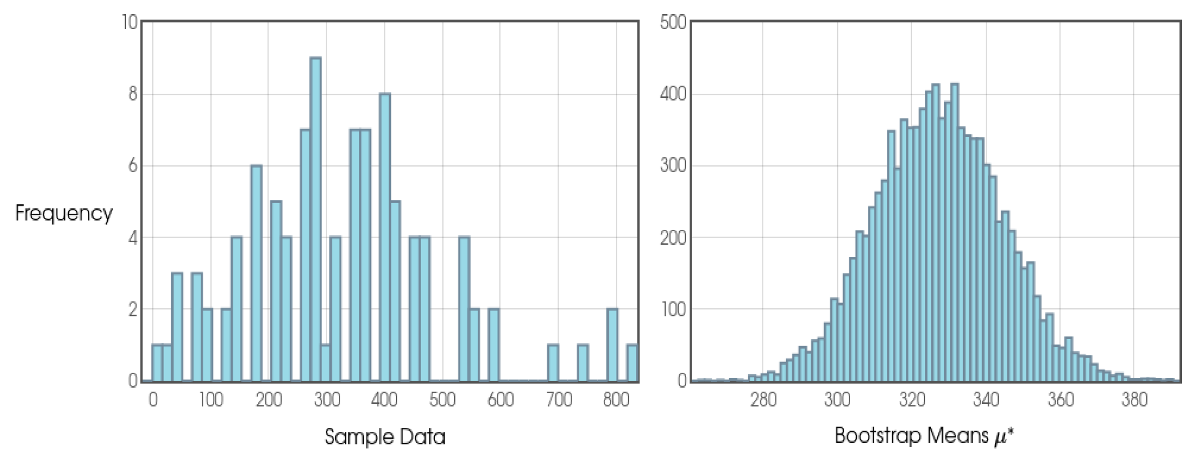
Table 30.
Analysis of the expected mean Profit and Loss scenario after 100 Future Values (FVs) considering the parameters φ = 1.02 k = 50 and j = 2.
Table 30.
Analysis of the expected mean Profit and Loss scenario after 100 Future Values (FVs) considering the parameters φ = 1.02 k = 50 and j = 2.
By analyzing the overall results of profit or loss in the 100 Future Values (FVs), we can see that when we apply the Bootstrap Confidence Interval considering a 95% level of reliability, we can expect the value of the true population mean to be between $293.89 and $361.66, that is, indicating a range of expected profitability values for the bettor. As we can see in Figure 21, in this case we can expect a behavior tending towards normal distribution from the values presented in the Shapiro-Wilk test.
4.1.1.2. Bankroll Considering the Configuration φ = 1.02, k = 50 and j = 2
Figure 22.
Graphical analysis of the expected mean bankroll scenario after 100 Future Values (FVs) considering the parameters φ = 1.02 k = 50 and j = 2.
Figure 22.
Graphical analysis of the expected mean bankroll scenario after 100 Future Values (FVs) considering the parameters φ = 1.02 k = 50 and j = 2.
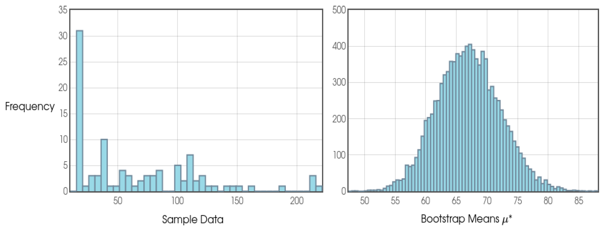
Table 31.
Analysis of the expected mean bankroll scenario after 100 Future Values (FVs) considering the parameters φ = 1.02 k = 50 and j = 2.
Table 31.
Analysis of the expected mean bankroll scenario after 100 Future Values (FVs) considering the parameters φ = 1.02 k = 50 and j = 2.
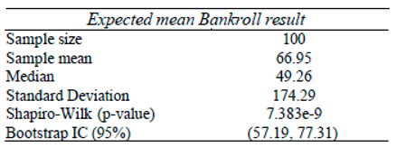
With regard to the analysis from the point of view of the amount of average financial value expected for a bettor to have in his bankroll in such a way that it is possible to cover all possible periods of volatility and remain in the game until the end of the intermediate blocks and their respective small blocks.
We can see in Figure 22 that the amounts available for the player's bankroll follow an asymmetrical distribution to the right, i.e. it is more likely that when we simulate 100 next “Future Values” (FVs), the bettor will only need to have, in the hypothetical example considering the initial parameters, an initial bankroll of just $20, which is enough to cover 2 small blocks jn with a positive final result until the bettor already has enough resources to follow all the sequences of small blocks within all Intermediate Blocks. In this example, a bankroll of just $20 would be enough for 31 scenarios out of 100 analyzed.
We can say that, when analyzed from the point of view of the average obtained after 10,000 simulations using the Bootstrap method, we can expect with 95% confidence that the true population average is between $57.19 and $77.31, which could therefore be an interesting starting point for a bettor to keep in mind the amount of money needed - considering that each stake is $10 - so that Victoria can be employed throughout the trajectory and survive the effects of the expected natural volatility.
4.1.1.3. ROI Considering the Configuration φ = 1.02, k = 50 and j = 2
Figure 23.
Graphical analysis of the expected mean ROI scenario after 100 Future Values (FVs) considering the parameters φ = 1.02 k = 50 and j = 2.
Figure 23.
Graphical analysis of the expected mean ROI scenario after 100 Future Values (FVs) considering the parameters φ = 1.02 k = 50 and j = 2.
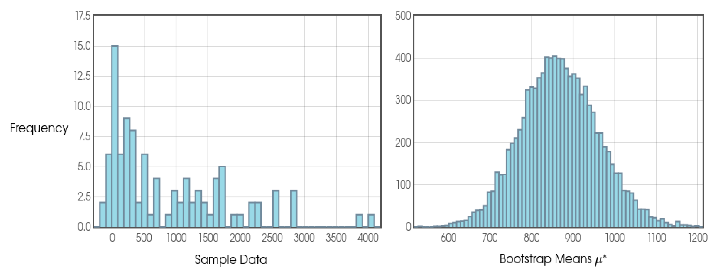
Table 32.
Analysis of the expected mean ROI scenario after 100 Future Values (FVs) considering the parameters φ = 1.02 k = 50 and j = 2.
Table 32.
Analysis of the expected mean ROI scenario after 100 Future Values (FVs) considering the parameters φ = 1.02 k = 50 and j = 2.
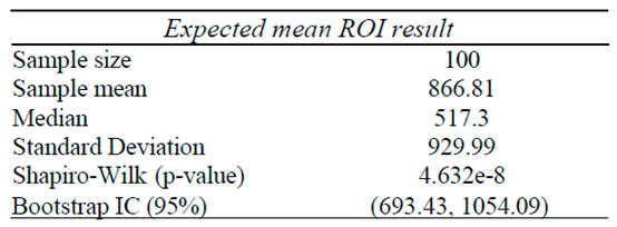
In this scenario, we evaluated the Return on Investment (ROI), i.e. by analyzing the final profit or loss for the sum of all the amounts invested along the way needed to cover all the periods of volatility up to the established time period. In this sense, over the course of “100 Future Values” the graphical analysis as a result found a pattern of behavior that does not follow a normal distribution and, we can say that we are 95% confident that the true population mean lies somewhere between 693.425% and 1054.091% of Return on Investment.
4.1.1.4. 0/2 Considering the Configuration φ = 1.02, k = 50 and j = 2
Figure 24.
Graphical analysis of the small blocks scenario Jn = 0 expected mean after 100 Future Values (FVs) considering the parameters φ = 1.02 k = 50 and j = 2.
Figure 24.
Graphical analysis of the small blocks scenario Jn = 0 expected mean after 100 Future Values (FVs) considering the parameters φ = 1.02 k = 50 and j = 2.
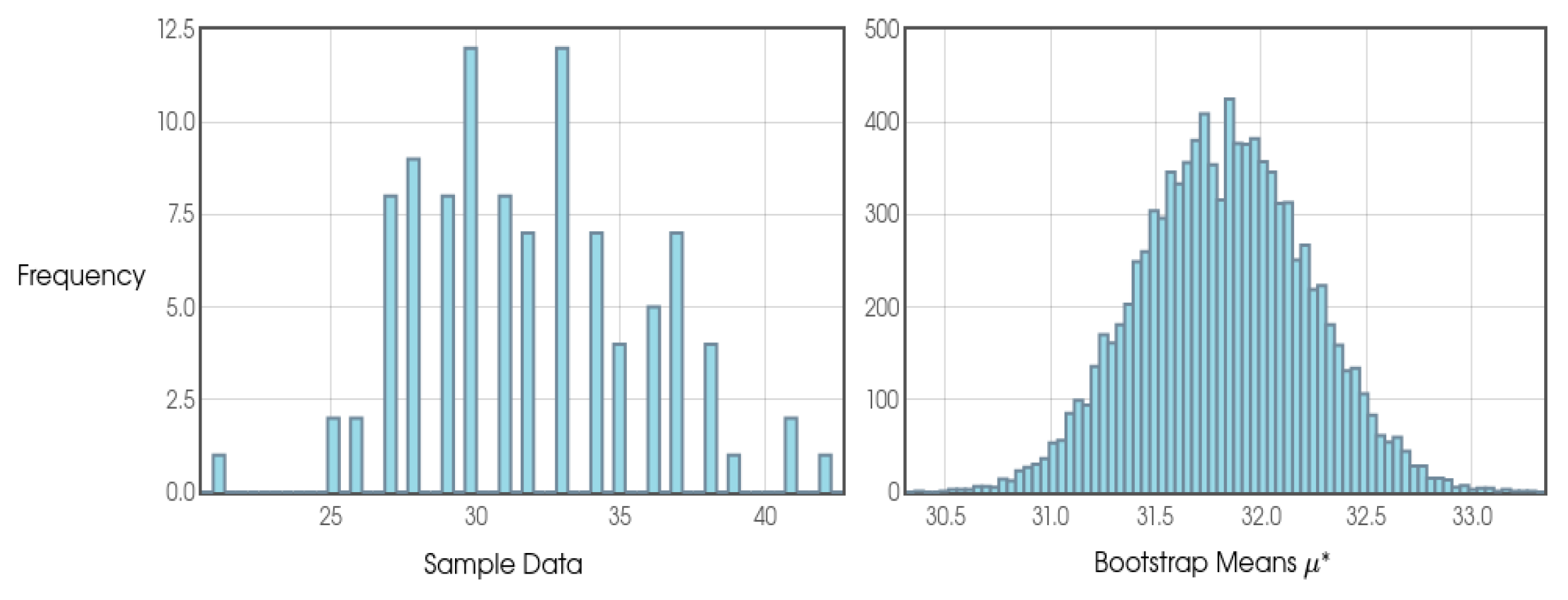
Table 33.
Analysis of the small blocks scenario Jn = 0 expected mean after 100 Future Values (FVs) considering the parameters φ = 1.01 k = 50 and j = 2.
Table 33.
Analysis of the small blocks scenario Jn = 0 expected mean after 100 Future Values (FVs) considering the parameters φ = 1.01 k = 50 and j = 2.
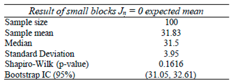
With regard to the number of Small Blocks (jn) containing 0 positive results, that is, with 0 successful small blocks, after analyzing 100 Intermediate Blocks (IBs) we are 95% confident that the true population mean lies somewhere between 31.05 and 32.61 Intermediate blocks containing values equal to 0. It is as if we entered this game knowing that as n goes to infinity, the values of 0 present in Intermediate Blocks (out of a total of 2 possible small blocks) will converge to approximately 32%.
4.1.1.5. 1/2 Considering the Configuration φ = 1.02, k = 50 and j = 2
Figure 25.
Graphical analysis of the small blocks scenario Jn = 1 expected mean after 100 Future Values (FVs) considering the parameters φ = 1.02 k = 50 and j = 2.
Figure 25.
Graphical analysis of the small blocks scenario Jn = 1 expected mean after 100 Future Values (FVs) considering the parameters φ = 1.02 k = 50 and j = 2.
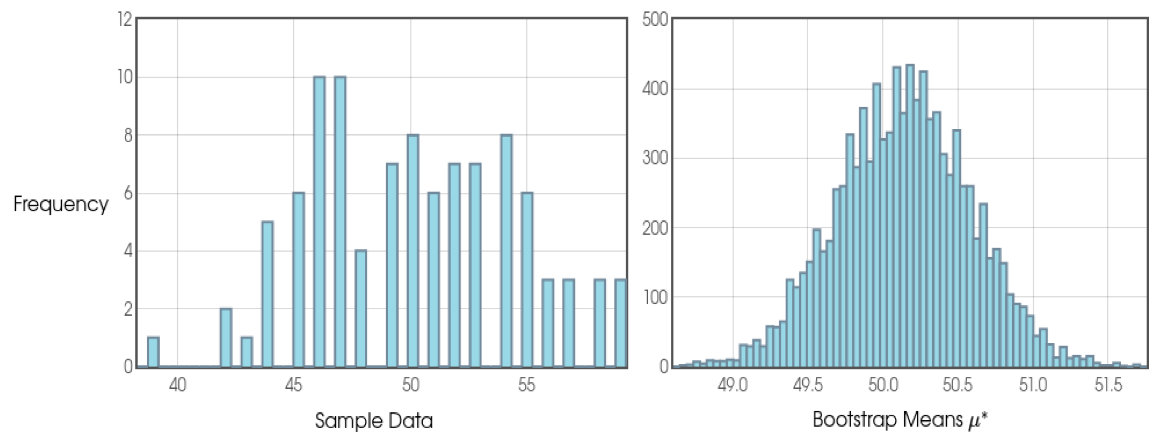
Table 34.
Analysis of the small blocks scenario Jn = 1 expected mean after 100 Future Values (FVs) considering the parameters φ = 1.02 k = 50 and j = 2.
Table 34.
Analysis of the small blocks scenario Jn = 1 expected mean after 100 Future Values (FVs) considering the parameters φ = 1.02 k = 50 and j = 2.
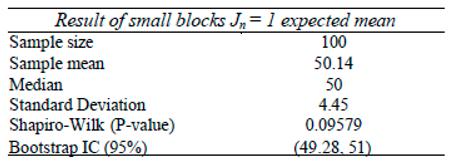
With regard to the number of Small Blocks (jn) containing 1 positive result, that is, with 1 successful small block, after analyzing 100 Intermediate Blocks (IBs) we are 95% confident that the true population mean lies somewhere between 49.28 and 51 Intermediate blocks containing values equal to 1. It is as if we entered this game knowing that as n goes to infinity, the values of 1 small block of success (out of a total of 2 possible small blocks) present in Intermediate Blocks will converge to approximately 50%.
4.1.1.6. 2/2 Considering the Configuration φ = 1.02, k = 50 and j = 2
Figure 26.
Graphical analysis of the small blocks scenario Jn = 2 expected mean after 100 Future Values (FVs) considering the parameters φ = 1.02 k = 50 and j = 2.
Figure 26.
Graphical analysis of the small blocks scenario Jn = 2 expected mean after 100 Future Values (FVs) considering the parameters φ = 1.02 k = 50 and j = 2.
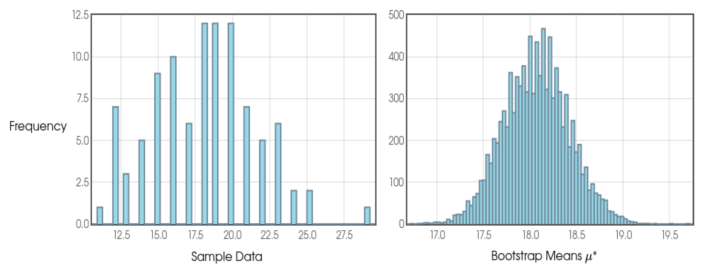
Table 35.
Analysis of the small blocks scenario Jn = 2 expected mean after 100 Future Values (FVs) considering the parameters φ = 1.02 k = 50 and j = 2.
Table 35.
Analysis of the small blocks scenario Jn = 2 expected mean after 100 Future Values (FVs) considering the parameters φ = 1.02 k = 50 and j = 2.
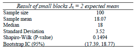
With regard to the number of small blocks containing 2 positive results, that is, with 2 small blocks of successes, after analyzing 100 Intermediate Blocks (IBs) we are 95% confident that the true population mean lies somewhere between 17.39 and 18.77 Intermediate Blocks containing values equal to 2. It is as if we went into this game knowing that as n goes to infinity the values of the 2 small blocks of success (out of a total of 2 possible small blocks) present in Intermediate Blocks will converge to approximately 18%.
4.1.2. Analysis of the Results for the Configuration φ = 1.04; j = 3 and k = 33
With this configuration, we theoretically expect to have 99 games (j*k), which in practice means we can expect somewhere between 48 and 70 games (or k independent events) to be bet on in each Intermediate Block (IB). With this configuration with φ = 1.04; j = 3 and k = 33, for example, we can expect an oscillation up or down of an average of 5,900 games for each FV.
Again, throughout this study, random numbers between 1 and 1,000 were drawn from sources such as Random.Org, GIGACalcultator, and ANU QRNG. Furthermore, again, in order to provide better graphic visualization of this study, the stats.blue platform was considered, as well as standard data visualization using the R language. This time, we can classify a Small Block (jn) as successful (β) if in the sequence of 33 numbers generated (understood as 33 independent events occurring) all the numbers are equal to or greater than 40. Similarly, if there are numbers equal to or less than 39 in the middle of the sequence, we say that we have a Small Failure Block (ζi), meaning that a bettor has lost a bet along the way.
Again, the following is a reminder of Victoria's formulation:
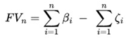 where,
IB =[(S0 φ k– S0) βi] – S0 ζi
φ = odd / probability of success of the event k = Time Period
S0 = Initial Value (fixed value used for each independent event)
βi = "Success" blocks. That is, the cost/benefit ratio compared to the investment in each stake in each n game is positive and there is some profit.
ζi = "Failure" blocks. That is, the cost/benefit ratio compared to the investment in each stake iin each n game is negative and there is some loss.
If we consider a fixed stake of $10 for each k independent events, when we put it into Victoria's formulation we will see that if we have no successful blocks among the three possible Small Blocks (jn) of each IB, we will therefore have a loss of -$30. If we have one successful Small Block (β) and two unsuccessful ones (ζ), the net result will be a modest but important profit of $6.48.
Considering a scenario in which we have 2 Small Blocks of success and only 1 of failure, we can expect a positive net return of $42.97. Although it happens less often than other combinations, if we have 3 Small Blocks of success (β) and none of failure (ζ), in just one IB, the bettor can expect a positive net result of $79.45.
Through Table 36, Table 37, Table 38 and Table 39, Figure 27 and as the FV43 simulation can also be consulted in the supplementary material for this study, we can see that only a $20 bankroll was needed, which in this example corresponds to just two stakes for the bettor to make constant profits by simply 'reinvesting' the profit for new bets and generating even more profit.
Table 36.
Analysis of the FV43 with the parameters φ = 1.04; j = 3 and k = 33 Part I.
| FV43 | 0/3 | P/L | β / ζ |
|---|---|---|---|
| IB1 | 1 | $6.48 | β |
| IB2 | 2 | $42.97 | β |
| IB3 | 1 | $6.48 | β |
| IB4 | 2 | $42.97 | β |
| IB5 | 1 | $6.48 | β |
| IB6 | 0 | -$30.00 | ζ |
| IB7 | 3 | $79.45 | β |
| IB8 | 1 | $6.48 | β |
| IB9 | 2 | $42.97 | β |
| IB10 | 0 | -$30.00 | ζ |
| IB11 | 2 | $42.97 | β |
| IB12 | 1 | $6.48 | β |
| IB13 | 0 | -$30.00 | ζ |
| IB14 | 0 | -$30.00 | ζ |
| IB15 | 1 | $6.48 | β |
| IB16 | 1 | $6.48 | β |
| IB17 | 2 | $42.97 | β |
| IB18 | 2 | $42.97 | β |
| IB19 | 2 | $42.97 | β |
| IB20 | 0 | -$30.00 | ζ |
| IB21 | 1 | $6.48 | β |
| IB22 | 2 | $42.97 | β |
| IB23 | 1 | $6.48 | β |
| IB24 | 2 | $42.97 | β |
| IB25 | 1 | $6.48 | β |
| Σ | $380.98 |
Table 37.
Analysis of the FV43 with the parameters φ = 1.04; j = 3 and k = 33 Part II.
| FV43 | 0/3 | P/L | β / ζ |
|---|---|---|---|
| IB26 | 2 | $42.97 | β |
| IB27 | 0 | -$30.00 | ζ |
| IB28 | 1 | $6.48 | β |
| IB29 | 0 | -$30.00 | ζ |
| IB30 | 1 | $6.48 | β |
| IB31 | 2 | $42.97 | β |
| IB32 | 1 | $6.48 | β |
| IB33 | 2 | $42.97 | β |
| IB34 | 1 | $6.48 | β |
| IB35 | 2 | $42.97 | β |
| IB36 | 0 | -$30.00 | ζ |
| IB37 | 1 | $6.48 | β |
| IB38 | 1 | $6.48 | β |
| IB39 | 2 | $42.97 | β |
| IB40 | 1 | $6.48 | β |
| IB41 | 2 | $42.97 | β |
| IB42 | 2 | $42.97 | β |
| IB43 | 0 | -$30.00 | ζ |
| IB44 | 0 | -$30.00 | ζ |
| IB45 | 1 | $6.48 | β |
| IB46 | 1 | $6.48 | β |
| IB47 | 1 | $6.48 | β |
| IB48 | 0 | -$30.00 | ζ |
| IB49 | 2 | $42.97 | β |
| IB50 | 1 | $6.48 | β |
| Σ | $235.04 |
Table 38.
Analysis of the FV43 with the parameters φ = 1.04; j = 3 and k = 33 Part III.
| FV43 | 0/3 | P/L | β / ζ |
|---|---|---|---|
| IB51 | 1 | $6.48 | β |
| IB52 | 0 | -$30.00 | ζ |
| IB53 | 2 | $42.97 | β |
| IB54 | 2 | $42.97 | β |
| IB55 | 0 | -$30.00 | ζ |
| IB56 | 3 | $79.45 | β |
| IB57 | 1 | $6.48 | β |
| IB58 | 0 | -$30.00 | ζ |
| IB59 | 1 | $6.48 | β |
| IB60 | 2 | $42.97 | β |
| IB61 | 0 | -$30.00 | ζ |
| IB62 | 0 | -$30.00 | ζ |
| IB63 | 1 | $6.48 | β |
| IB64 | 0 | -$30.00 | ζ |
| IB65 | 1 | $6.48 | β |
| IB66 | 1 | $6.48 | β |
| IB67 | 0 | -$30.00 | ζ |
| IB68 | 1 | $6.48 | β |
| IB69 | 0 | -$30.00 | ζ |
| IB70 | 1 | $6.48 | β |
| IB71 | 1 | $6.48 | β |
| IB72 | 2 | $42.97 | β |
| IB73 | 2 | $42.97 | β |
| IB74 | 0 | -$30.00 | ζ |
| IB75 | 0 | -$30.00 | ζ |
| Σ | $52.62 |
Table 39.
Analysis of the FV43 with the parameters φ = 1.04; j = 3 and k = 33 Part IV.
| FV43 | 0/3 | P/L | β / ζ |
|---|---|---|---|
| IB76 | 0 | -$30.00 | ζ |
| IB77 | 3 | $79.45 | β |
| IB78 | 1 | $6.48 | β |
| IB79 | 1 | $6.48 | β |
| IB80 | 1 | $6.48 | β |
| IB81 | 2 | $42.97 | β |
| IB82 | 0 | -$30.00 | ζ |
| IB83 | 2 | $42.97 | β |
| IB84 | 0 | -$30.00 | ζ |
| IB85 | 2 | $42.97 | β |
| IB86 | 1 | $6.48 | β |
| IB87 | 0 | -$30.00 | ζ |
| IB88 | 2 | $42.97 | β |
| IB89 | 0 | -$30.00 | ζ |
| IB90 | 1 | $6.48 | β |
| IB91 | 1 | $6.48 | β |
| IB92 | 1 | $6.48 | β |
| IB93 | 0 | -$30.00 | ζ |
| IB94 | 1 | $6.48 | β |
| IB95 | 1 | $6.48 | β |
| IB96 | 2 | $42.97 | β |
| IB97 | 1 | $6.48 | β |
| IB98 | 0 | -$30.00 | ζ |
| IB99 | 0 | -$30.00 | ζ |
| IB100 | 1 | $6.48 | β |
| Σ | $125.58 |
We can say that FV43, in general, presented a very comfortable scenario for this hypothetical bettor, in which it basically showed very little volatility throughout each Small Block and their respective Intermediate Blocks, as we can see in Figure 27. As a result of this FV we had a positive result of $794.22 which generated an ROI of 3,871.10%. This is a dream scenario for a victorian bettor, since Bob, for example, would have made an average profit of $ 0.1346 cents per ticket if we consider that Bob had to bet on 5,900 independent events in this FV.
Figure 27.
Graphical analysis of profit or loss of FV43 with parameters φ = 1.04; j = 3 and k = 33.
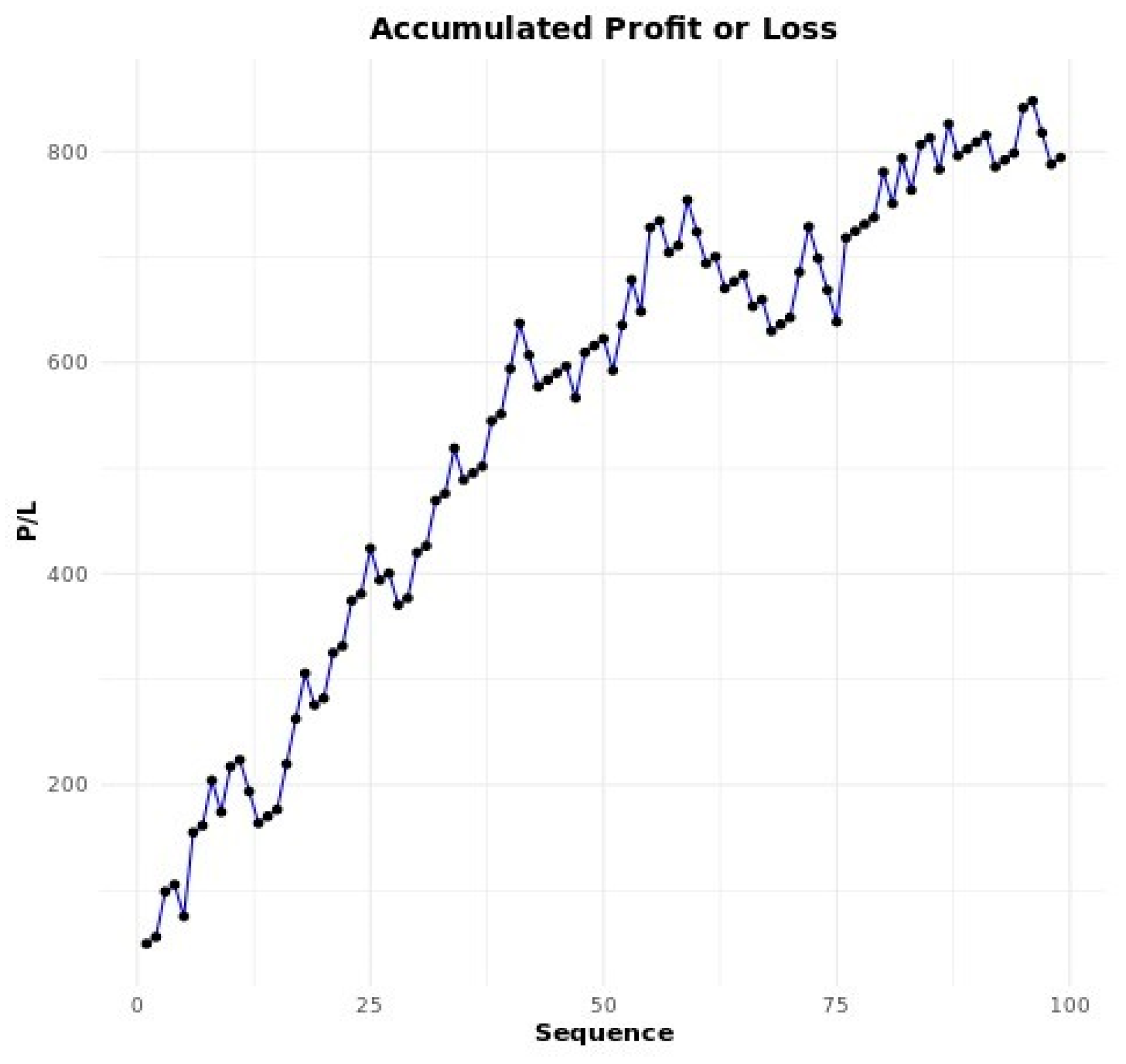
In the same way as we analyzed the configuration in the previous section, we will analyze the results of another 100 hypothetical FVs in order to possibly check which category this configuration φ = 1.04; j = 3 and k = 33 would belong to in the Victoria model.
Table 40.
Analysis of 100 FVs with parameters φ = 1.04; j = 3 and k = 33 Part I.
| FVn | 0/3 | 1/3 | 2/3 | 3/3 | β / 100 | P/L | Bankroll | ROI |
|---|---|---|---|---|---|---|---|---|
| FV1 | 22 | 58 | 18 | 2 | 78/100 | $648.20 | $77.04 | 741.38% |
| FV2 | 27 | 46 | 25 | 2 | 73/100 | $721.23 | $60.00 | 1102.05% |
| FV3 | 27 | 45 | 25 | 3 | 73/100 | $794.20 | $60.00 | 1223.67% |
| FV4 | 28 | 46 | 23 | 3 | 72/100 | $684.74 | $60.00 | 1041.23% |
| FV5 | 31 | 48 | 17 | 4 | 69/100 | $429.33 | $40.56 | 958.51% |
| FV6 | 29 | 48 | 21 | 2 | 71/100 | $502.31 | $60.00 | 737.18% |
| FV7 | 24 | 53 | 21 | 2 | 76/100 | $684.71 | $30.00 | 2182.37% |
| FV8 | 29 | 47 | 22 | 2 | 71/100 | $538.80 | $113.52 | 374.63% |
| FV9 | 29 | 49 | 18 | 3 | 71/100 | $459.15 | $30.00 | 1430.50% |
| FV10 | 30 | 47 | 19 | 4 | 70/100 | $538.60 | $90.00 | 498.44% |
| FV11 | 23 | 52 | 21 | 4 | 77/100 | $886.92 | $77.04 | 1051.25% |
| FV12 | 30 | 51 | 18 | 1 | 70/100 | $283.21 | $30.00 | 844.03% |
| FV13 | 32 | 49 | 16 | 3 | 68/100 | $283.23 | $209.27 | 35.34% |
| FV14 | 29 | 54 | 15 | 2 | 71/100 | $283.22 | $98.16 | 188.53% |
| FV15 | 30 | 42 | 26 | 2 | 70/100 | $647.99 | $30.00 | 2059.97% |
| FV16 | 29 | 46 | 22 | 3 | 71/100 | $611.55 | $60.00 | 919.25% |
| FV17 | 34 | 47 | 14 | 5 | 66/100 | $283.25 | $158.16 | 79.09% |
| FV18 | 27 | 52 | 17 | 4 | 73/100 | $575.08 | $115.19 | 399.24% |
| FV19 | 32 | 41 | 24 | 3 | 68/100 | $575.07 | $53.52 | 974.5% |
| FV20 | 32 | 47 | 19 | 2 | 68/100 | $319.70 | $47.04 | 579.63% |
| FV21 | 26 | 49 | 21 | 4 | 74/100 | $757.48 | $85.20 | 789.06% |
| FV22 | 25 | 56 | 16 | 3 | 75/100 | $538.59 | $30.00 | 1695.3% |
| FV23 | 27 | 49 | 19 | 5 | 73/100 | $721.01 | $90.00 | 701.01% |
| FV24 | 28 | 42 | 26 | 4 | 72/100 | $866.92 | $60.00 | 1344.87% |
| FV25 | 25 | 43 | 27 | 5 | 75/100 | $1,085.81 | $30.00 | 3519.37% |
| Σ | - | - | - | - | - | $14,720.30 | - | - |
Table 41.
Analysis of 100 FVs with parameters φ = 1.04; j = 3 and k = 33 Part II.
| FVn | 0/3 | 1/3 | 2/3 | 3/3 | β / 100 | P/L | Bankroll | ROI |
|---|---|---|---|---|---|---|---|---|
| FV26 | 28 | 48 | 20 | 4 | 72/100 | $648.04 | $89.27 | 625.93% |
| FV27 | 31 | 43 | 21 | 5 | 69/100 | $648.05 | $67.43 | 861.07% |
| FV28 | 30 | 44 | 22 | 4 | 70/100 | $648.21 | $90.00 | 620.23% |
| FV29 | 36 | 43 | 19 | 2 | 64/100 | $173.78 | $62.60 | 177.6% |
| FV30 | 33 | 46 | 19 | 2 | 67/100 | $283.41 | $53.52 | 429.54% |
| FV31 | 32 | 42 | 26 | 0 | 68/100 | $429.38 | $30.00 | 1331.27% |
| FV32 | 26 | 52 | 18 | 4 | 74/100 | $648.22 | $83.52 | 676.13% |
| FV33 | 25 | 49 | 21 | 5 | 75/100 | $867.14 | $83.52 | 938.24% |
| FV34 | 29 | 44 | 23 | 4 | 71/100 | $721.23 | $30.00 | 2304.1% |
| FV35 | 24 | 53 | 18 | 5 | 76/100 | $794.15 | $30.00 | 2547.17% |
| FV36 | 32 | 47 | 19 | 2 | 68/100 | $319.89 | $30.00 | 966.3% |
| FV37 | 22 | 52 | 22 | 4 | 78/100 | $940.10 | $77.04 | 1120.28% |
| FV38 | 30 | 42 | 26 | 2 | 70/100 | $647.58 | $47.04 | 1276.66% |
| FV39 | 33 | 40 | 26 | 1 | 67/100 | $465.87 | $218.10 | 113.6% |
| FV40 | 31 | 51 | 17 | 1 | 69/100 | $210.42 | $78.66 | 167.51% |
| FV41 | 35 | 47 | 17 | 4 | 65/100 | $302.85 | $211.65 | 43.09% |
| FV42 | 31 | 47 | 21 | 1 | 69/100 | $356.38 | $30.00 | 1087.93% |
| FV43 | 29 | 41 | 27 | 3 | 71/100 | $794.21 | $60.00 | 1223.68% |
| FV44 | 31 | 45 | 21 | 3 | 69/100 | $502.33 | $94.07 | 434% |
| FV45 | 32 | 49 | 16 | 3 | 68/100 | $283.39 | $30.00 | 844.63% |
| FV46 | 33 | 47 | 18 | 2 | 67/100 | $246.92 | $97.41 | 153.49% |
| FV47 | 28 | 47 | 24 | 1 | 72/100 | $575.29 | $103.88 | 453.8% |
| FV48 | 28 | 55 | 13 | 4 | 72/100 | $392.81 | $123.36 | 218.43% |
| FV49 | 34 | 40 | 24 | 2 | 66/100 | $429.38 | $93.75 | 358.01% |
| FV50 | 32 | 43 | 24 | 1 | 68/100 | $429.37 | $30.00 | 1331.23% |
| Σ | - | - | - | - | - | $12,758.40 | - | - |
Table 42.
Analysis of 100 FVs with parameters φ = 1.04; j = 3 and k = 33 Part III.
| FVn | 0/3 | 1/3 | 2/3 | 3/3 | β / 100 | P/L | Bankroll | ROI |
|---|---|---|---|---|---|---|---|---|
| FV51 | 29 | 43 | 24 | 4 | 71/100 | $757.72 | $30.00 | 2425.73% |
| FV52 | 35 | 39 | 23 | 3 | 65/100 | $429.38 | $116.85 | 267.46% |
| FV53 | 26 | 49 | 20 | 5 | 74/100 | 794.17 | $47.04 | $1588.29% |
| FV54 | 29 | 45 | 25 | 1 | 71/100 | $575.30 | $107.04 | 437.46% |
| FV55 | 22 | 54 | 23 | 1 | 78/100 | $757.68 | $44.63 | 1597.69% |
| FV56 | 36 | 39 | 21 | 4 | 64/100 | $392.89 | $30.00 | 1209.63% |
| FV57 | 37 | 41 | 19 | 3 | 63/100 | $210.46 | $137.04 | 53.58% |
| FV58 | 35 | 46 | 18 | 1 | 65/100 | $100.99 | $59.27 | 70.39% |
| FV59 | 36 | 38 | 25 | 1 | 64/100 | $319.94 | $201.11 | 59.09% |
| FV60 | 26 | 51 | 18 | 5 | 74/100 | $721.19 | $30.00 | 2303.97% |
| FV61 | 30 | 52 | 16 | 2 | 70/100 | $283.38 | $64.07 | 342.3% |
| FV62 | 31 | 47 | 21 | 1 | 69/100 | $356.38 | $30.00 | 1087.93% |
| FV63 | 29 | 45 | 25 | 1 | 71/100 | $575.30 | $40.56 | 1318.39% |
| FV64 | 33 | 42 | 21 | 4 | 67/100 | $502.33 | $53.52 | 838.58% |
| FV65 | 35 | 42 | 21 | 2 | 65/100 | $283.43 | $167.03 | 69.69% |
| FV66 | 28 | 51 | 19 | 2 | 72/100 | $465.81 | $87.59 | 431.81% |
| FV67 | 35 | 44 | 20 | 1 | 65/100 | $173.97 | $201.12 | -13.5% |
| FV68 | 30 | 42 | 24 | 4 | 70/100 | $721.24 | $47.03 | 1433.57% |
| FV69 | 37 | 41 | 18 | 4 | 63/100 | $246.94 | $81.11 | 204.45% |
| FV70 | 29 | 44 | 23 | 5 | 71/100 | $800.68 | $30.00 | 2568.93% |
| FV71 | 33 | 43 | 22 | 2 | 67/100 | $392.88 | $167.04 | 135.2% |
| FV72 | 35 | 42 | 18 | 5 | 65/100 | $392.87 | $47.04 | 735.18% |
| FV73 | 25 | 51 | 23 | 1 | 75/100 | $648.24 | $53.52 | 1111.21% |
| FV74 | 22 | 53 | 20 | 5 | 78/100 | $940.09 | $107.04 | 778.26% |
| FV75 | 34 | 48 | 17 | 1 | 66/100 | $100.98 | $158.10 | -36.13% |
| Σ | - | - | - | - | - | $11,944.24 | - | - |
Table 43.
Analysis of 100 FVs with parameters φ = 1.04; j = 3 and k = 33 Part IV.
| FVn | 0/3 | 1/3 | 2/3 | 3/3 | β / 100 | P/L | Bankroll | ROI |
|---|---|---|---|---|---|---|---|---|
| FV76 | 32 | 51 | 16 | 1 | 68/100 | $137.45 | $143.52 | -4.23 |
| FV77 | 35 | 46 | 15 | 4 | 65/100 | $210.43 | $302.56 | -30.45 |
| FV78 | 31 | 42 | 25 | 2 | 69/100 | $575.31 | $40.56 | 1318.42 |
| FV79 | 36 | 45 | 14 | 5 | 64/100 | $210.43 | $64.08 | 228.39 |
| FV80 | 28 | 54 | 15 | 3 | 72/100 | $392.82 | $123.32 | 218.54 |
| FV81 | 38 | 40 | 18 | 4 | 62/100 | $210.46 | $224.62 | -6.3 |
| FV82 | 28 | 47 | 20 | 5 | 72/100 | $721.21 | $184.08 | 291.79 |
| FV83 | 32 | 49 | 19 | 0 | 68/100 | $173.86 | $117.75 | 47.65 |
| FV84 | 31 | 39 | 27 | 3 | 69/100 | $721.26 | $30.00 | 2304.2 |
| FV85 | 29 | 48 | 21 | 2 | 71/100 | $502.31 | $70.55 | 611.99 |
| FV86 | 26 | 53 | 17 | 4 | 74/100 | $611.73 | $47.04 | 1200.45 |
| FV87 | 31 | 51 | 17 | 1 | 69/100 | $30.00 | $601.40 | 210.42 |
| FV88 | 30 | 46 | 18 | 6 | 70/100 | $648.24 | $30.00 | 2060.8 |
| FV89 | 35 | 48 | 16 | 2 | 65/100 | $107.46 | $117.60 | -8.62% |
| FV90 | 31 | 43 | 21 | 5 | 69/100 | $648.26 | $30.00 | 2060.87% |
| FV91 | 38 | 39 | 21 | 2 | 62/100 | $174.02 | $251.46 | -30.78% |
| FV92 | 31 | 43 | 24 | 2 | 69/100 | $538.82 | $30.00 | 1696.07% |
| FV93 | 27 | 45 | 27 | 1 | 73/100 | $721.24 | $30.00 | 2304.13 |
| FV94 | 28 | 45 | 24 | 3 | 72/100 | $719.88 | $30.00 | 2299.60% |
| FV95 | 26 | 45 | 27 | 2 | 74/100 | $829.34 | $30.00 | 2664.47% |
| FV96 | 26 | 57 | 16 | 1 | 74/100 | $356.33 | $60.00 | 493.88% |
| FV97 | 31 | 50 | 16 | 3 | 69/100 | $319.87 | $207.59 | 54.09% |
| FV98 | 26 | 50 | 21 | 3 | 74/100 | $684.72 | $60.00 | 1041.20% |
| FV99 | 35 | 47 | 13 | 5 | 65/100 | $210.42 | $143.52 | 46.61% |
| FV100 | 32 | 47 | 18 | 3 | 68/100 | $356.37 | $68.15 | 422.92% |
| Σ | - | - | - | - | - | $10,992.66 | - | - |
From Table 40, Table 41, Table 42 and Table 43, after analyzing all 100 FVs, we can see that we made a total profit of $50,415.60. If we consider that we would have an average of 5,900 games for each FV, this would give us a total of 590,000 games, which would give us an average profit of $0.0855 cents for each ticket wagered.
Also according to Table 40, Table 41, Table 42 and Table 43, if we consider a Yellow Zone = 20, that is, multiply by the first standard profit, in this case $6.48, we get a YZ = 129.60, meaning that all values equal to or less than these as final results in an FV should be classified in the so-called Yellow Zone, which shows us a warning sign because the profit was not so attractive. Using these reference values, for example, we found that FV58, FV75, FV87 and FV89 belong to the Yellow Zone.
As we can also see, we didn't have any FVs indicating any negative results, however, due to the fact that this is a seminal study, we also have to be careful about flagging as a possible configuration belonging to the “singularity point” category, i.e. a configuration that will always be 100% regardless of the number of each group of 100 FVs simulated.
From the point of view of the experience I've had in this field of randomness, from Monte Carlo simulations to those physical games with a globe that simulate a lottery, as much as the results have indicated something positive in terms of the average profit in each FV and the fact that there are no FVs with a negative result, we can probably expect this configuration to belong to the 94% or 95% category, indicating that we'll probably have a maximum of 5 or 6 FVs with a negative result.
4.2.1.1. PL Considering the Configuration φ = 1.04, k = 33 and j = 3
Figure 28.
Graphical analysis of the expected mean Profit and Loss Scenario after 100 Future Values (FVs) considering the parameters φ = 1.04 k = 33 and j = 3.
Figure 28.
Graphical analysis of the expected mean Profit and Loss Scenario after 100 Future Values (FVs) considering the parameters φ = 1.04 k = 33 and j = 3.
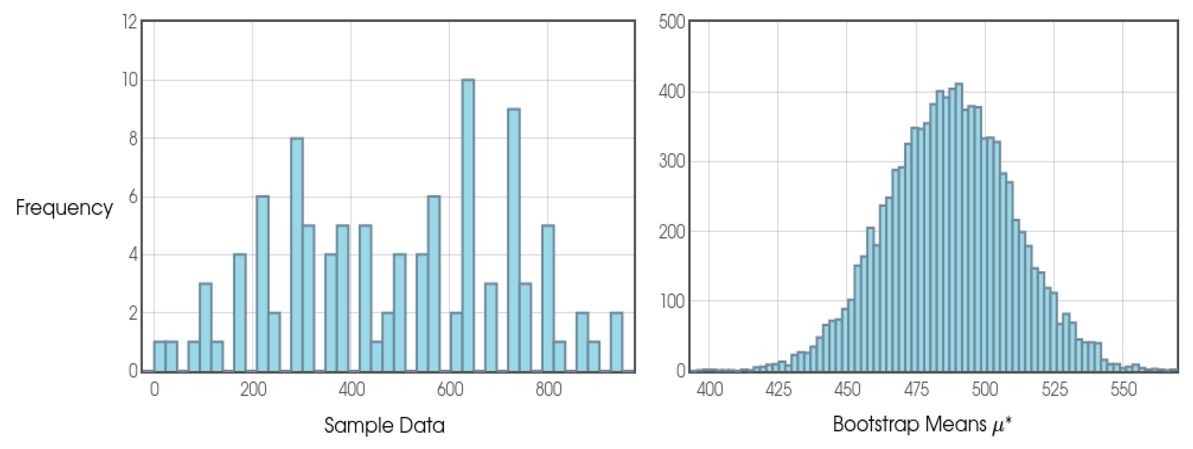
Table 44.
Analysis of the expected mean Profit and Loss scenario after 100 Future Values (FVs) considering the param-eters φ = 1.04 k = 33 and j = 3.
Table 44.
Analysis of the expected mean Profit and Loss scenario after 100 Future Values (FVs) considering the param-eters φ = 1.04 k = 33 and j = 3.
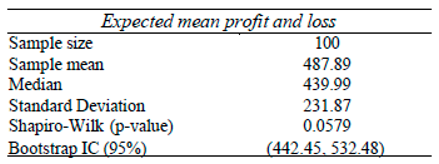
By analyzing the overall results of profit or loss in the 100 Future Values (FVs), we can see that when we apply the Bootstrap Confidence Interval considering a 95% level of reliability, we can expect the value of the true population mean to be between $442.45 and $532.48, i.e. indicating a range of expected profitability values for the bettor.
4.2.1.2. Bankroll Considering the Configuration φ = 1.04, k = 33 and j = 3
Figure 29.
Graphical analysis of the expected mean bankroll scenario after 100 Future Values (FVs) considering the parameters φ = 1.04 k = 33 and j = 3.
Figure 29.
Graphical analysis of the expected mean bankroll scenario after 100 Future Values (FVs) considering the parameters φ = 1.04 k = 33 and j = 3.
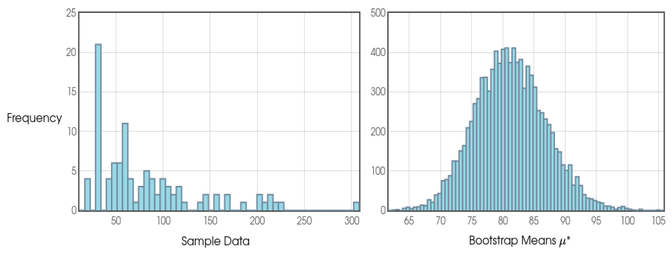
Table 45.
Analysis of the expected mean bankroll scenario after 100 Future Values (FVs) considering the parameters φ = 1.04 k = 33 and j = 3.
Table 45.
Analysis of the expected mean bankroll scenario after 100 Future Values (FVs) considering the parameters φ = 1.04 k = 33 and j = 3.
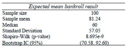
Again, when it comes to analyzing the bankroll, we see that the normal distribution is far from the expected distribution. Our interpretation of the results is that we are 95% confident that the true population mean lies somewhere between $70.58 and $92.60. Therefore, a bettor should expect to have something in this range of available value if each stake is $10.
4.2.1.3. ROI Considering the Configuration φ = 1.04, k = 33 and j = 3
Figure 30.
Graphical analysis of the expected mean ROI scenario after 100 Future Values (FVs) considering the parameters φ = 1.04 k = 33 and j = 3.
Figure 30.
Graphical analysis of the expected mean ROI scenario after 100 Future Values (FVs) considering the parameters φ = 1.04 k = 33 and j = 3.
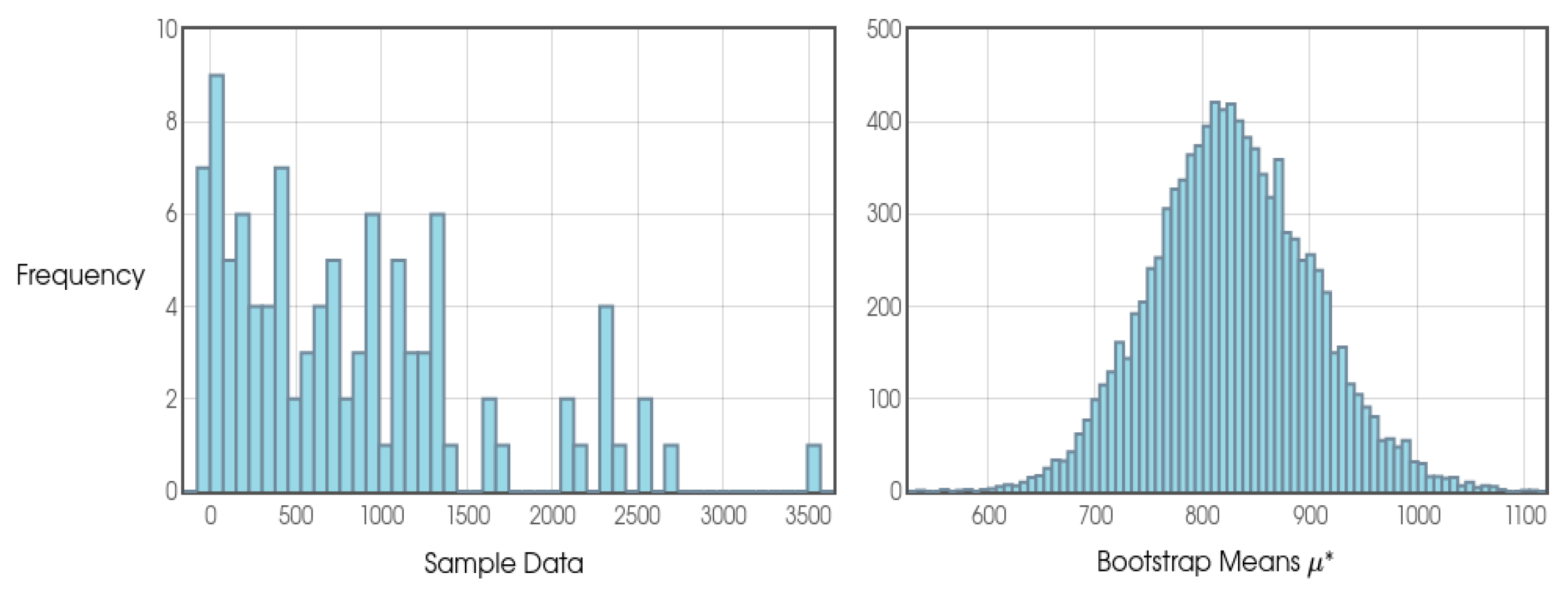
Table 46.
Analysis of the expected mean ROI with scenario after 100 Future Values (FVs) considering the parameters φ = 1.04 k = 33 and j = 3.
Table 46.
Analysis of the expected mean ROI with scenario after 100 Future Values (FVs) considering the parameters φ = 1.04 k = 33 and j = 3.
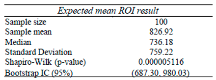
Regarding ROI we can say that we are 95% confident that the true population mean lies somewhere between 687.2955% and 980.0319% return on the bettor’s investiment.
4.2.1.4. 0/3 Considering the Configuration φ = 1.04, k = 33 and j = 3
As can be seen below, with regard to the number of small blocks containing 0 positive results, that is, with 0 successful small blocks, after analyzing 100 Intermediate Blocks (IBs) we are 95% confident that the true population mean lies somewhere between 29.36 and 30.85 Intermediate Blocks containing values equal to 0. It is as if we entered this game knowing that as n goes to infinity the values of 0 present in Intermediate Blocks (out of a total of 3 possible small blocks) will converge to approximately 30%.
Figure 31.
Graphical analysis of the small blocks scenario Jn = 0 expected mean after 100 Future Values (FVs) considering the parameters φ = 1.04 k = 33 and j = 3.
Figure 31.
Graphical analysis of the small blocks scenario Jn = 0 expected mean after 100 Future Values (FVs) considering the parameters φ = 1.04 k = 33 and j = 3.
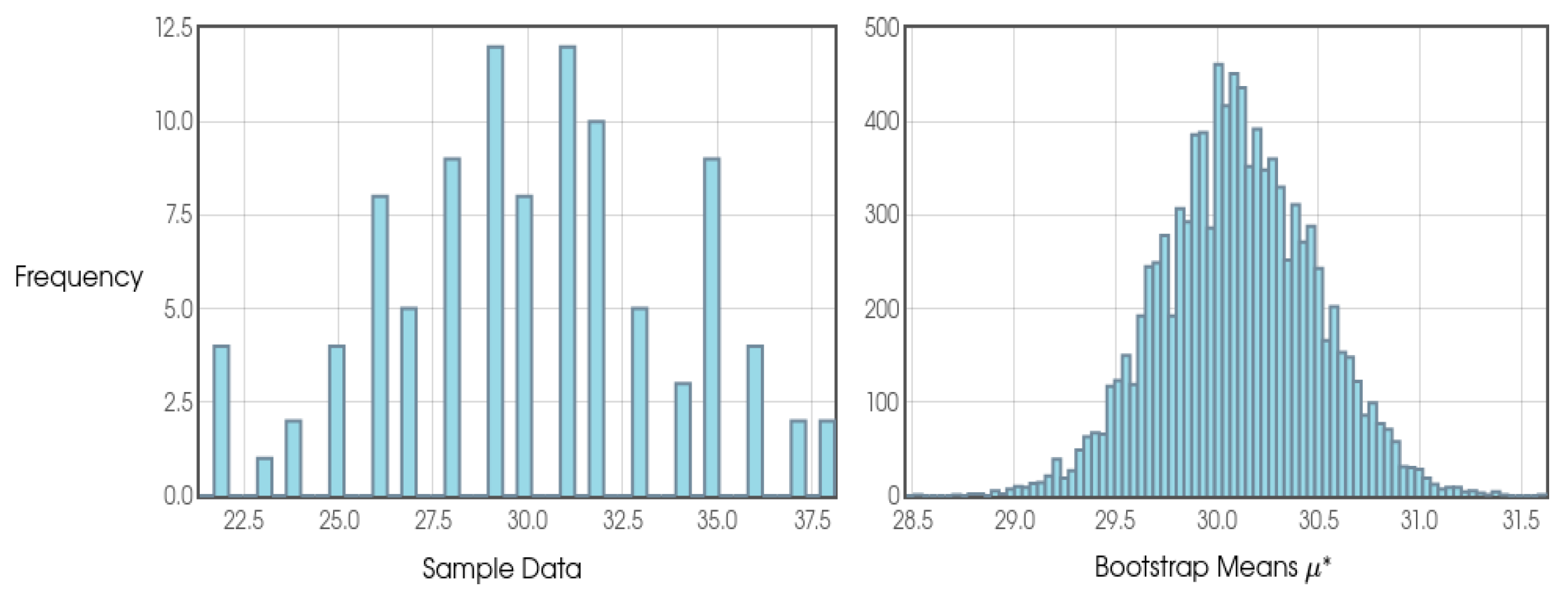
Table 47.
Analysis of the small blocks scenario Jn = 0 expected mean after 100 Future Values (FVs) considering the pa-rameters φ = 1.04 k = 33 and j = 3.
Table 47.
Analysis of the small blocks scenario Jn = 0 expected mean after 100 Future Values (FVs) considering the pa-rameters φ = 1.04 k = 33 and j = 3.
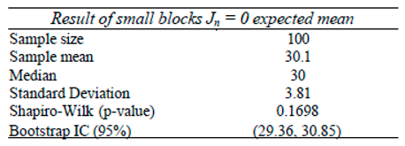
4.2.1.5. 1/3 Considering the Configuration φ = 1.04, k = 33 and j = 3
With regard to the number of small blocks containing 1 positive result, that is, with 1 small block of success, after analyzing 100 Intermediate Blocks (IB s) we are 95% confident that the true population mean lies somewhere between 45.80 and 47.56 Intermediate Blocks containing values equal to 1. It is as if we entered this game knowing that as n goes to infinity, the values of 1 small block of success (out of a total of 3 possible small blocks) present in Intermediate Blocks will converge to approximately 46%, for example.
Figure 32.
Graphical analysis of the small blocks scenario Jn = 1 expected mean after 100 Future Values (FVs) considering the parameters φ = 1.04 k = 33 and j = 3.
Figure 32.
Graphical analysis of the small blocks scenario Jn = 1 expected mean after 100 Future Values (FVs) considering the parameters φ = 1.04 k = 33 and j = 3.
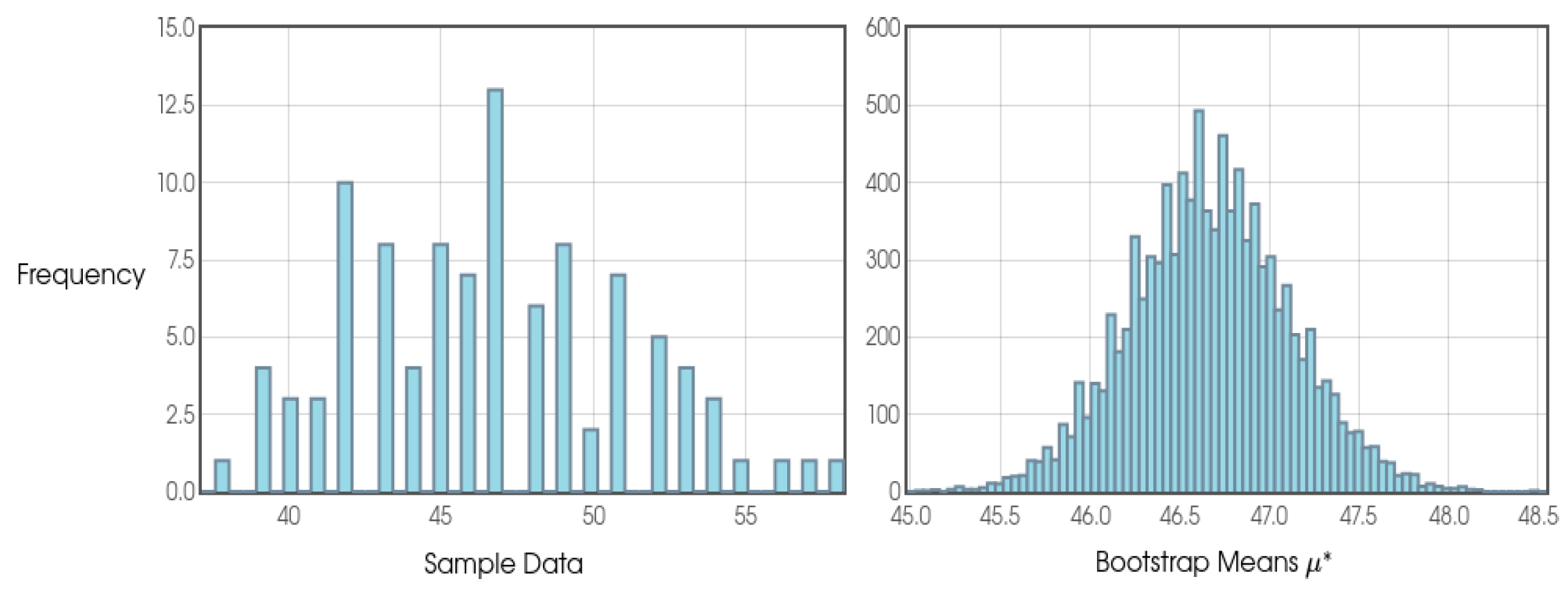
Table 48.
Analysis of the small blocks scenario Jn = 1 expected mean after 100 Future Values (FVs) considering the pa-rameters φ = 1.04 k = 33 and j = 3.
Table 48.
Analysis of the small blocks scenario Jn = 1 expected mean after 100 Future Values (FVs) considering the pa-rameters φ = 1.04 k = 33 and j = 3.
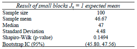
4.2.1.6. 2/3 Considering the Configuration φ = 1.04, k = 33 and j = 3
With regard to the number of small blocks containing 2 positive results, that is, with 2 small blocks of successes, after analyzing 100 Intermediate Blocks (IBs) we are 95% confident that the true population mean lies somewhere between 19.70 and 21.09 Intermediate Blocks containing values equal to 2. It is as if we entered this game knowing that as n goes to infinity, the values of the 2 small blocks of success (out of a total of 3 possible small blocks) present in each Intermediate Block will converge to approximately 20%, for example.
Figure 33.
Graphical analysis of the small blocks scenario Jn = 2 expected mean after 100 Future Values (FVs) considering the parameters φ = 1.04 k = 33 and j = 3.
Figure 33.
Graphical analysis of the small blocks scenario Jn = 2 expected mean after 100 Future Values (FVs) considering the parameters φ = 1.04 k = 33 and j = 3.
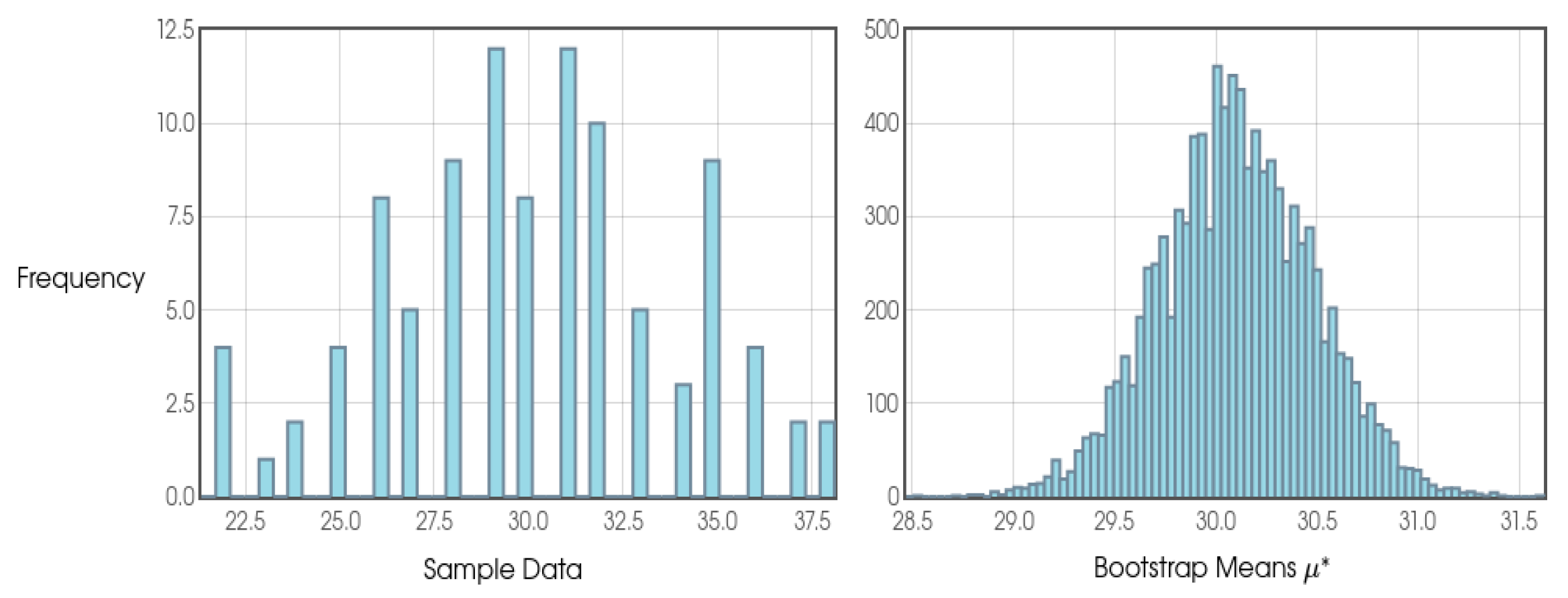
Table 49.
Analysis of the small blocks scenario Jn = 2 expected mean after 100 Future Values (FVs) considering the pa-rameters φ = 1.04 k = 33 and j = 3.
Table 49.
Analysis of the small blocks scenario Jn = 2 expected mean after 100 Future Values (FVs) considering the pa-rameters φ = 1.04 k = 33 and j = 3.
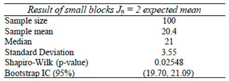
4.2.1.7. 3/3 Considering the Configuration φ = 1.04, k = 33 and j = 3
With regard to the number of small blocks containing 3 positive results, that is, with 3 small blocks of successes, after analyzing 100 Intermediate Blocks (IBs) we are 95% confident that the true population mean lies somewhere between 2.59 and 3.15 Intermediate Blocks containing values equal to 3. It is as if we entered this game knowing that as n goes to infinity, the values of the 3 small blocks of success (out of a total of 3 possible small blocks) present in each Intermediate Block will converge to approximately 3%, for example.
Figure 34.
Graphical analysis of the small blocks scenario Jn = 3 expected mean after 100 Future Values (FVs) considering the parameters φ = 1.04 k = 33 and j = 3.
Figure 34.
Graphical analysis of the small blocks scenario Jn = 3 expected mean after 100 Future Values (FVs) considering the parameters φ = 1.04 k = 33 and j = 3.
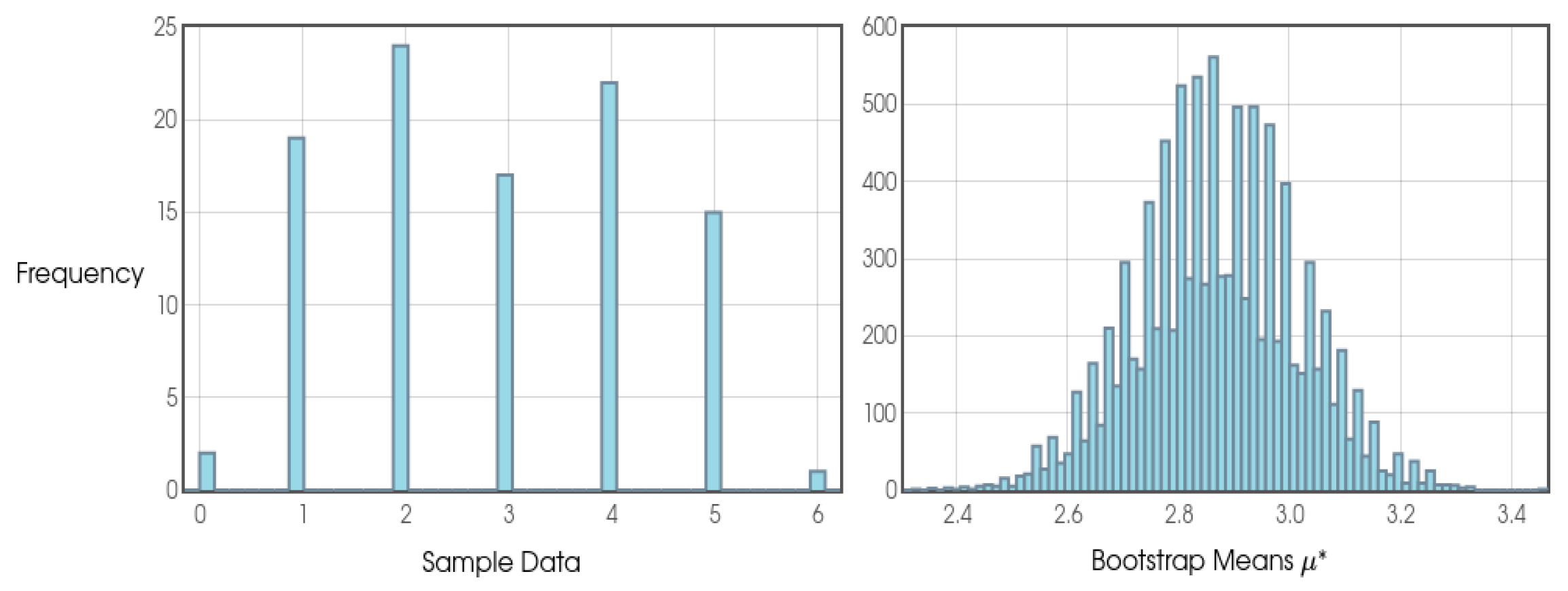
Table 50.
Analysis of the small blocks scenario Jn = 3 expected mean after 100 Future Values (FVs) considering the pa-rameters φ = 1.04 k = 33 and j = 3.
Table 50.
Analysis of the small blocks scenario Jn = 3 expected mean after 100 Future Values (FVs) considering the pa-rameters φ = 1.04 k = 33 and j = 3.
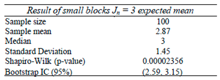
4.3. Some Reflections on Victoria
These potential profits that can be made by Victoria are justified for a number of reasons, including the understanding that winning and losing is part of the expected process according to probability theory itself, so what really matters is that we deliberately look for a set of strategies in which we have a positive mathematical expectation in the long term. In the case of Victoria, it is enough that the probabilities defined by the sportsbooks are equal to the probabilities defined by the individual, reflecting the “real” probabilities expected by the event.
Unlike the Kelly Criterion, there is no need, in principle, for the player to guarantee some percentage advantage over the house, even taking into account possible fees (vigorish), since the model already takes this scenario into account. In fact, if a bettor using the Victoria method wanted to take into account a percentage advantage over the house, we can logically expect much better results than would be obtained using Victoria in its pure essence. In this sense, we could also expect that those configurations defined as belonging to the 90%, 95%, 97%... categories could be strong candidates for always belonging to the 100% parameter category in each FV considered, meaning that the punter will be able to obtain an assured profitability within the approximately 4800 to 7000 games wagered on each Future Value (FV), reducing the mathematically necessary time and being more applicable to the real world.
Another point to bear in mind is that, as we saw earlier in the results section, Victoria doesn't require a strong bankroll, as the hierarchies of Small Blocks (jn), Intermediate Blocks (IBs) and Future Values (FVs) already create a natural barrier against the effect of volatility, which, with well-defined φ, j and k configurations, can provide a positive trend with long-term profits for the victorian bettor.
Furthermore, the application of compound interest or logarithmic growth present in Victoria's formulation is what allows a victorian bettor to have positive mathematical expectation against the house. We also say that in this case, the function η(Xt) the complementary action in the description of this function is the understanding of the behavior of randomness added to the mathematical formulation of Victoria itself and its designs of φ, j, and k containing compound interest (with the idea of reinvestment), for example.
Although it is sometimes considered obvious due to the knowledge acquired over the years with the development of statistics and computer science, it is necessary to make it clear and intelligible that the nature of the random number generator, be it PRNGs, QuasiRNGs, TRNGs, or QRNGs, doesn't matter to us either, except for the probability distribution observed behind each of them. It is the probability distribution that dictates the rules of the game.
Of course, in the case of PRNGs and QuasiRNGs, for example, there are additional issues arising from their deterministic nature, such as the size of the cycle (for those PRNGs considered non-periodic) and the case of the seeds, which can influence the level of entropy and other statistical qualities. However, what we must bear in mind is that, in principle, there are no statistically significant differences between a good PRNG and a QRNG.
If we know and master the basic properties of randomness given a probability distribution, we can have good control and obtain a “partial prediction of the future” and, among other things, we can reduce the number of possible combinations to achieve a certain result. This means that, in principle, if we take information security, for example, through a uniform probability distribution, we can have positive and negative surprises in the future, both with new security implementation measures and with the possible use of these measurable random structures for illicit purposes.
Today, we are not yet fully able to delve into randomness and its basic structuring in certain probability distributions, but that doesn't mean that it won't be possible in the coming years to expand the initial concept of the “predictable random component” even further, especially with the help of artificial intelligence and quantum technology.
4.3.1. Limitations
4.3.1.1. Data-Driven Decision Making
As in the field of time series analysis, Victoria's application will depend on the existence of a database containing a historical series of at least a few variables specific to the event that will occur. There is no other way to go but to make decisions based on data and statistics.
This method can take time to analyze the data and check whether the odds offered by the sportsbooks are consistent with the data in the historical series. We can therefore say the user must have the ability to carry out analysis in a similar way to what sportsbooks already do. And this is nothing new in the world of sports trading, since bettors who are part of the small slice of constantly profitable users, (usually between 1% and 5%) already do these analyses, as Sumpter (2020) pointed out when he demonstrated the logistic regression formula is one of the 10 main formulas that shape the world as we know it. Well, in the case of the world of sports trading, logistic regression is extremely useful for analyzing whether a particular sporting event has value or not according to the odds presented by the sportsbooks.
4.3.1.2. The Chaotic Nature of Sporting Events
Sporting events, by their very nature, are very chaotic, which can make it difficult to make a more accurate prediction in terms of odds, especially if the user places a bet on a live event, since events in progress can be more susceptible to imbalances in the odds both for and against the prospects expected by the user: betting market conditions can change, and new factors can emerge, affecting the accuracy of predictions. Therefore, when applying Victoria it is best to have already carried out an analysis and made an entry action before the event starts.
We need to bear in mind that when it comes to sporting events, there are countless variables that can sometimes have a significant influence and/or be difficult to quantify, such as: the weather variable (heat, cold, rain, snow...), terrain (altitude level), the time of the game and the way the visiting team travels (plane, bus...), emotional issues arising from each individual player, the atmosphere inside the stadium, such as chants from the fans, injuries to a player, taunts from the rival team, officiating errors, among other possible scenarios.
4.3.1.3. The Uncertainty Factor Will Remain Forever
It should also be clear and understandable that the very nature of probability does not provide us with an exact probability and/or a series of intervals from point a or b in which they will always be directed towards the expected values of the lower or upper limit. What Probability Theory does tell us is that there is a strong tendency for the results to converge to these expected probabilities p given a margin of error ± ε.
Even in terms of current bibliographical references, there is common agreement in references on the subject of Probability Theory that, although such expected results are an extremely small probability to the point that they basically don't exist and, if they occur, could take thousands and thousands, billions and billions of years, among other longer time scales, the uncertainty factor, sometimes also referred to as “random noise”, will persist in the face of our data, which could lead to an undesirable result occurring in the future.
4.3.1.4. Psychological Biases and Sortsbook Control Actions
As also discussed in the course of the study, psychological/emotional biases coupled with the actions of some sportsbooks, such as limiting the markets available for betting, limiting the amounts wagered, and even blocking consistently winning bettors, are possibilities that can prevent a strategy with positive mathematical expectations from lasting in the long term.
It is also known that there are few sportsbook groups that operate through a business model aimed exclusively at professional bettors, so although they are already used to dealing with players who are constant winners in the long term, the introduction of Victoria and victorian players could change this scenario and the uncertainties regarding the possible actions of these sportsbooks also tend to be uncertain.
4.3.1.5. A New Approach
Victoria is an innovative approach and will therefore require further complementary studies evaluating the different types of configurations as well as the overall results in terms of Future Values (FVs) from the perspective of convergence in probabilities.
Knowing these natural laws converted into probabilities and their respective distributions, we can say that past results don't guarantee future results either, but they do tend to show us a strong trend of what might happen. This is how sportsbooks and professional sports traders work, spending most of their lives living in the dice paradise, that is, through data and statistics.
4.4. Some Reflections on the Victoria-Nash Asymmetric Equilibrium (VNAE)
The Victoria-Nash Asymmetric Equilibrium (VNAE) expands game theory by modeling equilibria in asymmetric information and strategy scenarios. Unlike the traditional Nash equilibrium, where no player has a unilateral incentive to deviate, the VNAE allows agents to gain a sustainable long-term advantage by exploiting predictable patterns in randomness, represented by the function fv(Xt). Its application extends to stochastic, zero-sum, asymmetric, repeated and imperfect information games, and can be seen as an extension of Nash, Stackelberg and Bayesian equilibria.
Structural advantages, knowledge and experience added to the rational aspect of exploring patterns in true randomness to extract some value can be said to be a primary basis of the Victoria-Nash Asymmetric Equilibrium.
In VNAE, players have different capacities for identification, prediction and adaptation, making it possible to model scenarios in which some players better exploit the patterns in the randomness 'embedded' in the game and which is available to all players.
Unlike the Stackelberg equilibrium, the VNAE does not presuppose a fixed hierarchy, although it can reflect structural advantages in certain contexts, as can be seen in contexts such as social inequalities. Its main characteristic comes from a player's ability to identify and exploit hidden patterns in the true randomness given a probability distribution - uniform distribution being adopted as the standard in this study - making the function fv(Xt) not just an 'optimal strategy', but a fundamental basis for many types of games, which justifies in this study its being treated as a new basic function in game theory.
As we saw in section 2.10 “Is it possible to beat the house?” we see some examples of how throughout history scientists and people have beaten the house using partially predictable randomness as part of their optimal strategies. As we are dealing with the randomness factor given a probability distribution, we say that it is something timeless, so if there are no changes to the rules of the game, the same people who beat the house in the past will also beat it in the present and future. In this sense, even if we consider that the house adopts defensive actions such as limitations and blocking the accounts of victorian players, the tendency is that it will not converge to a Nash Equilibrium, since the fundamental and original structure of the game has been altered. Although this example is applied to the world of betting, scenario I, as seen in section 3.6.3, continues to stand out.
The Victoria-Nash Asymmetric Equilibrium (VNAE) reveals a new perspective in Decision Theory and Game Theory, where strategic asymmetry can be exploited to obtain sustainable advantages in different systems. Furthermore, this model provides a mathematical basis for explaining natural, economic and social inequalities, showing how small strategic advantages amplify over time, making it possible to model asymmetries in social interactions, business negotiations and geopolitical disputes, helping to understand and influence these phenomena.
In finance, the methodology can be applied to optimize decisions in risky markets, identifying strategies that maximize statistically favorable returns. In this sense, it can be an important tool for decision-making in financial trading and sports betting, for example. Similarly, in Artificial Intelligence, the concept can be used to develop adaptive agents that adjust their strategies in dynamic environments, exploiting statistical biases in a similar way to traders and automated decision systems.
In addition to economics and technology, the VNAE, as in Hubbell's (2001) approach, is applied to the natural sciences, modeling dynamic and stochastic processes in physics, explaining strategic advantages in natural selection and describing, in ecology, how competition between species shapes patterns of biodiversity and resource distribution.
The fv(Xt) function shows great flexibility when modeling natural, political, social and economic phenomena, but it can have some limitations. The model assumes that agents have rationality, access to information and the ability to manage it, which may not be realistic in all contexts. Furthermore, its application in areas such as biology and social sciences may require specific adaptations.
Another limitation involves the computational factor, as data storage and processing can be barriers for some players. In addition to statistical knowledge, it is necessary to manage randomness through some physical system such as suitable hardware or software. If poorly modeled, randomness and its results can introduce biases.
In fact, there are different interpretations of the partial prediction of true randomness, some might argue that hitting a random number at a certain point is a random event, impossible to predict. Nowadays, this is true. However, it should be clear and understandable here that the “Predictable Random Component” should be visualized and understood through convergence in probabilities (in more depth from various angles) and not exactly the prediction of certain specific points within the randomness of a uniform distribution, for example.
With the knowledge we have today, this more specific predictability is something of a limitation, but it doesn't mean that over the years, with advances in quantum technology and artificial intelligence, as well as advances in statistics itself, this won't be achievable either. But, in principle, the basis of the VNAE lies in the convergence of probabilities.
Despite some possible limitations inherent in the model, as well as those present in others, in general, the VNAE tends to be a robust model for explaining asymmetric advantages which both the author and the academic community are invited to discuss and put into practice in their respective experiments to disseminate new results by solving real problems.
5. Conclusions
In the context of sports betting and financial markets, the Victoria methodology demonstrates that, under certain strategic parameters, it is possible to obtain sustainable statistical advantages. The analysis of the convergence of positive FVs suggests that players or investors can manage risks more efficiently, reducing losses and maximizing gains. However, its application requires strict control over variables such as capital allocation, time series analysis and appropriate probabilistic modeling, ensuring that the theoretical benefits of the model are effectively translated into practical results.
Based on Victoria's formulation, applied in sports betting contexts, a new function η(Xt) called the “Predictable Random Component” was presented in the context of Decision Theory and Game Theory. It is a function that considers that through true randomness we can extract patterns, which are based on convergences in probabilities that, added to other complementary actions, whether through a mathematical operation, physics or any other cognitive action, can provide asymmetric advantages for one of the sides in a given game.
In this study, the following configurations were used φ = 1.02 k = 50 and j = 2 and φ = 1.04 k = 33 and j = 3 in the Monte Carlo simulation. Each standard stake was also assumed to be $10. At the end of the study, both configurations were shown to probably belong to the category of at least 94% or 95% positive FVs over a sequence of every 100 FVs. As this is a seminal study, we hope to obtain more data in this regard in the future through new practical studies.
As for the first configuration (φ = 1.02 k = 50 and j = 2), among the main results over 100 FVs we had $325.03 in average profit (between $296.89 and $361.66 in the Bootstrap Interval with 95% confidence). As for the expected bankroll to play the game, we had an average of $66.95 (between $57.19 and $77.31 in the Bootstrap Interval with 95% confidence). And we had an average ROI of 866.81% (between 693.43% and 1,054.09% in the Bootsrap Interval with 95% confidence). Considering that in this configuration we can expect an average of ± 6,500 games for each Future Value (FV), this gives us a positive mathematical expectation of approximately $0.05 cents for each betting ticket (k independent events).
As for the second configuration (φ = 1.04 k = 33 and j = 3), among the main results over 100 FVs we had $487.89 in average profit (between $442.45 and $532.48 in the Bootstrap Interval with 95% confidence). In addition, in terms of the expected bankroll to play the game, we had an average of $81.24 (between $70.58 and $92.60) in the Bootstrap Interval with 95% confidence). And, we had an average ROI of 826.92% (between 687.30% and 980.03% in the Bootstrap Interval with 95% confidence). Considering that in this configuration we can expect an average of ± 5,900 games for each Future Value (FV), this gives us a positive mathematical expectation of approximately $0.08269 cents for each betting ticket (k independent events).
According to the theorizing proposed in this study, both configurations tended to belong to what was presented in Part III of Teather of Dreams. Furthermore, a question that remains open in this study is the so-called “point of singularity” in which it is claimed that there may be optimal configurations of φ, j and k capable of always offering 100 positive FVs over groups of 100 FVs using only the Victoria formulation considering that the odds offered are considered “fair” without any margins of advantage for the bettor. If found in the future, this will certainly allow a much shorter period of time (number of independent k events) to mathematically ensure a positive result in a single FV.
Furthermore, as presented in Plays II and IV, it sounds like an interesting strategy to work by mixing the Victoria formulation with some possible margin for the player against the house, since it will take advantage of the positive mathematical expectation of the model, as well as reducing the number of games needed to mathematically eliminate all possible losses with some FV with a negative result.
As presented in Teather of Dreams in “Play V: Beacon Hill Park” and consequently in section 3.4, a theorem was presented as well as its respective proof demonstrating that as the number of games wagered increases, the gambler tends to mathematically eradicate all possible ways of having a negative result through the Law of Large Numbers and convergences in probability. In this case, what was presented in Play I and Play III could eliminate all possible forms of loss by increasing the number of small blocks (jn) reflected in the number of Intermediate Blocks (IBs) and even consider new designs beyond the standard originally proposed for amounts greater than 100 IBs in a FV.
Furthermore, this study proposed the concept of the Victoria-Nash Asymmetric Equilibrium (VNAE), an innovative approach that challenges the classical understanding of games dominated by randomness. Unlike the traditional Nash Equilibrium, the VNAE suggests that even in games with uniform distribution and dominant random factors at the base of the game, it is possible through the function η(Xt) or if you prefer, in this context, fv(Xt) to identify predictable patterns and exploit them in an asymmetric way, maintaining a continuous advantage over the opponent.
The relevance of this concept tends to extend beyond the field of sports betting and financial markets, with potential applications in areas such as social sciences (modeling geopolitical and business issues, social inequality, interpersonal relationships), cryptography, biology, medicine, artificial intelligence and dynamic systems, for example.
As a proof of the Victoria-Nash Asymmetric Equilibrium, Brouwer's fixed point theorem and Markov processes were used. Finally, although Victoria and VNAE offer a significant advance in the analysis of stochastic games and dynamic systems, their applications may require specific refinements depending on the context. Issues such as computational complexity, the need for robust data and assumptions about the rationality of agents must be taken into account. However, the contributions of these models point to a new paradigm in the modeling of randomness and strategy, offering promising mathematical tools for decision-making in stochastic environments. Furthermore, the author also concludes that only through data and Statistics can we 'beat' the house.
6. What Can We Expect Beyond Victoria and Victoria-Nash Asymmetric Equilibrium?
What should be clear and understandable both to my colleagues scientists, researchers as well as to readers in general is that this study is not about sports betting and the possibility of making profits in the medium and long run, as has been shown to be theoretically possible, but rather a deeper understanding of the behavior of true randomness given the tools available from the science of Statistics and Probability Theory.
Although at first it may seem counterintuitive, Victoria could open up new, similar approaches, focusing on the creation of new batteries of randomness tests that could complement the existing ones, and which could take into account the randomness generated by the principles of quantum physics. As discussed by Bessey (2002) and pointed out by Postman (1992), technologies can have a bias, an ideological tendency at their base. However, another point to bear in mind is that in the natural world much of the knowledge, techniques, and technologies are at our disposal, but intentions come from people.
In addition to the field of cybersecurity, impacts may be visible in other fields of science, from sociology to the economic and biological sciences, especially with regard to medicine, in which colleagues in these areas will know much better than I do how to shape the problems and results proposed and found here to their respective realities.
What defeats us as human beings is the scale and unpredictability of events. As soon as this barrier is overcome, part by part, by the scientific community over the next years, we will surely find ourselves at another level of evolution as homo sapiens and, with that, who knows, we may make great discoveries.
References
- Abellán Sánchez, C. (2018). Quantum random number generators for industrial applications.
- Accardi, L., & Boukas, A. (2007). The quantum black-scholes equation. arXiv preprint arXiv:0706.1300.
- Akerlof, G. A. (1978). The market for “lemons”: Quality uncertainty and the market mechanism. In Uncertainty in economics (pp. 235-251). Academic Press.
- Akter, R., & Ahmed, P. (2019). Some Real-Life Applications of Dynamical Systems. Iconic Research and Engineering Journals, 2(7), 1-15.
- Altmann, A. Hal Stern (2004) "On the probability of winning a football game" American Statistical Association August 1991, Vo1.45, No. 3,179-183.
- Amado, C., Nunes, C., Sardinha, A., & Ediçoes, S. P. E. (2019). Análise Estatıstica de Dados Financeiros.
- Anscombe, F. J., & Aumann, R. J. (1963). A definition of subjective probability. Annals of mathematical statistics, 34(1), 199-205.
- Amuji, H. O. , Onwuegbuchunam, D. E., Okechukwu, B. N., Okeke, K. O., & Okere, K. K. (2024) Application of Game Theory in the Nigerian Electoral System.
- Aragay, N., Pijuan, L., Cabestany, À., Ramos-Grille, I., Garrido, G., Vallès, V., & Jovell-Fernández, E. (2021).
- Current addiction in youth: Online sports betting. Frontiers in psychiatry, 11, 590554.
- Aslam, M., & Arif, O. H. (2024). Simulating chi-square data through algorithms in the presence of uncertainty.
- Infinite Study.
- Aumann, R. J. (1974). Subjectivity and correlation in randomized strategies. Journal of mathematical Economics, 1(1), 67-96.
- Aumann, R. J. , & Shapley, L. S. (1994). Long-term competition—a game-theoretic analysis. In Essays in Game Theory: In Honor of Michael Maschler (pp. 1-15). New York, NY: Springer New York.
- Aumann, R. J., Maschler, M., Stearns, R. E. (1995). Repeated games with incomplete information. MIT press. Aumann, R. J. (2024). Irrationality in game theory. In INTERACTIVE EPISTEMOLOGY (pp. 335-350).
- Avigliano, C. H. H. (2014). Towards deterministic preparation of single Rydberg atoms and applications to quantum information processing (Doctoral dissertation, Université Pierre et Marie Curie-Paris VI; Universidad de Concepción (Chili)).
- Baars, Bernard J. (1997). In the Theater of Consciousness: A rigorous scientific theory of consciousness. Journal of Consciousness Studies, 4(4), 292-309.
- Baeza-Yates, R. A. (1995). Teaching algorithms. ACM SIGACT News, 26(4), 51-59.
- Babaei, M., & Farhadi, M. (2011). Introduction to secure PRNGs. International Journal of Communications, Network and System Sciences, 4(10), 616.
- Baker, R. D., & McHale, I. G. (2013). Optimal betting under parameter uncertainty: Improving the Kelly criterion.
- Decision Analysis, 10(3), 189-199.
- Bagui, S., & Mehra, K. L. (2024). The Stirling Numbers of the Second Kind and Their Applications.
- Bhattacharjee, K., & Das, S. (2022). A search for good pseudo-random number generators: Survey and empirical studies. Computer Science Review, 45, 100471.
- Baldwin, R. R., Cantey, W. E., Maisel, H., & McDermott, J. P. (1956). The optimum strategy in blackjack. Journal of the American Statistical Association, 51(275), 429-439.
- Balková, Ľ., Bucci, M., De Luca, A., Hladký, J.,; Puzynina, S. (2016). Aperiodic pseudorandom number generators based on infinite words. Theoretical Computer Science 647, 85–100. [CrossRef]
- Banach, S. (1922). Sur les opérations dans les ensembles abstraits et leur application aux équations intégrales. Fundamenta mathematicae, 3(1), 133-181.
- Banerjee, A. V., & Duflo, E. (2011). Poor economics: A radical rethinking of the way to fight global poverty. Public Affairs.
- Baratta, P., Bel, J., Beauchamps, S. G., & Carbone, C. (2023). COVMOS: a new Monte Carlo approach for galaxy clustering analysis. Astronomy & Astrophysics, 673, A1.
- Barbosa, S. L. , Rezende, S. F. L., & Versiani, A. F. (2014). Relationships and knowledge in the firm internationalization process. Revista de Administração, 49(1), 129-140.
- Barnsley, M. F. (2014). Fractals everywhere. Academic press.
- Barron, E. N. (2024). Game theory: an introduction. John Wiley & Sons.
- Bartoš, F., Sarafoglou, A., Godmann, H. R., Sahrani, A., Leunk, D. K., Gui, P. Y., ... & Wagenmakers, E. J. (2023). Fair coins tend to land on the same side they started: Evidence from 350,757 flips. arXiv preprint arXiv:2310.04153.
- Bartlett, A. A. (1993). The Arithmetic of Growth: Methods of Calculation. Population and Environment, 14(4), 359–387. http://www.jstor.org/stable/.
- Bauer-Mengelberg, S. (1965). Kurt Gödel. On formally undecidable propositions of Principia mathematica and related systems I. English translation of 4183 by B. Meltzer. Oliver & Boyd, Edinburgh and London1962, pp. 37–72. The Journal of Symbolic Logic, 30(3), 359-362.
- Bayer, D., & Diaconis, P. (1992). Trailing the dovetail shuffle to its lair. The Annals of Applied Probability, 294-313. Becher, V., Figueira, S., & Picchi, R. (2007). Turing’s unpublished algorithm for normal numbers. Theoretical Computer Science, 377(1-3), 126-138.
- Becher, V. (2012, June). Turing’s normal numbers: towards randomness. In Conference on Computability in Europe (pp. 35-45). Berlin, Heidelberg: Springer Berlin Heidelberg.
- Belair, J. (2025). Causal Inference in Statistics: With Exercises, Practice Projects, and R Code Notebooks (Unedited Draft).
- Bellhouse, D. (2007). The problem of Waldegrave. Electronic Journal for the History of Probability and Statistics, 3(2), 1-12.
- Benter, W. (2008). Computer based horse race handicapping and wagering systems: a report. In Efficiency of racetrack betting markets (pp. 183-198).
- Beranek, M., & Buscher, U. (2024). Pricing decisions in a two-period closed-loop supply chain game under asymmetric information and uncertainty. Flexible Services and Manufacturing Journal, 36(4), 1450-1502.
- Bernoulli, J. (1713). Ars Conjectandi.
- Bessey, K. A. (2002). A neo-Luddite perspective on the use of calculators and computers in mathematics education.
- Idaho State University.
- Bonovas, S., & Piovani, D. (2023). Simpson’s paradox in clinical research: A cautionary tale. Journal of Clinical Medicine, 12(4), 1633.
- Booth, P., Chadburn, R., Haberman, S., James, D., Khorasanee, Z., Plumb, R. H., & Rickayzen, B. (2020). Modern actuarial theory and practice. CRC Press.
- Borel, É. , Les probabilités dénombrables et leurs applications arithmétiques. Rendiconti del Circolo Matematico di Palermo, vol. 27 (1909), no. 1, pp. 247–271.
- Bortolossi, H. Garbugio, G. Sartini, B. Uma Introdução à Teoria Econômica dos Jogos. 2017. Bonits, N. (1996). Managing intellectual capital strategically.
- Bouchaffra, D., Ykhlef, F., Faye, B., Azzag, H., & Lebbah, M. (2024). Game Theory Meets Statistical Mechanics in Deep Learning Design. arXiv preprint arXiv:2410.12264, arXiv:2410.12264.
- Boutsioukis, N. (2023). Comparative Analysis of Pseudorandom Number Generators: Mersenne Twister, Middle Square Method, and Linear Congruential Generator through Dieharder Tests. Middle Square Method, and Linear Congruential Generator through Dieharder Tests (January 15, 2023).
- Buchdahl, J. Fixed Odds Sports Betting: Statistical Forecasting and Risk Management. 2003.
- Buckle, M., Huang, C. S. (2018). The Efficiency of Sport Betting Markets: An Analysis Using Arbitrage Trading within Super Rugby. International Journal of Sport Finance, 13(3).
- Buhagiar, R. , Cortis, D., & Newall, P. W. (2018). Why do some soccer bettors lose more money than others?
- Journal of Behavioral and Experimental Finance, 18, 85-93.
- Black, F., Scholes, M., 1973. The pricing of options and corporate liabilities. Journal of Political Economy 81, 637– 659.
- Blando. F, Z. From Wald to Schnorr: von Mises’ definition of randomness in the aftermath of Ville’s theorem.
- Studies in History and Philosophy of Science, 106, pp. 196-207.
- Blitzstein J., Hwang J., 2014, Introduction to Probability. Chapman & Hall/CRC Texts in Statistical Science, CRC Press/Taylor & Francis Group, https://books.google.com/books?id=ZwSlMAEACAAJ.
- Blum, L., Blum, M. and Shub, M. (1986), “A Simple Unpredictable Pseudo-Random Number Generator,” SIAM Journal on Computing 15 (2), 364–383.
- Blum, L., & Blum, M. (2022). A theory of consciousness from a theoretical computer science perspective: Insights from the Conscious Turing Machine. Proceedings of the National Academy of Sciences, 119(21), e2115934119.
- Blum, L., & Blum, M. (2024). AI Consciousness is Inevitable: A Theoretical Computer Science Perspective. arXiv preprint arXiv:2403.17101.
- Blyth, C. R. (1972). On Simpson's paradox and the sure-thing principle. Journal of the American Statistical Association, 67(338), 364-366.
- Brouwer, L. E. J. (1911). Über abbildung von mannigfaltigkeiten. Mathematische annalen, 71(1), 97-115. Brouwer, Maria. (2016). The Positive Sum Game Paper presented at 16 th Schumpeter Society Conference.
- Montreal.
- Brown, N. M., Killen, C. J., & Schneider, A. M. (2022). Application of Game Theory to Orthopaedic Surgery. The Journal of the American Academy of Orthopaedic Surgeons, 30(4), 155–160. https://doi.org/10.5435/JAAOS-.
- Campani, C. A., & Menezes, P. B. (2004). Teorias da aleatoriedade. Revista de Informática teórica e Aplicada, 11(2), 75-98.
- Campolieti, G., & Makarov, R. N. (2018). Financial mathematics: a comprehensive treatment. Chapman and Hall/CRC.
- Cardano, G. (1965) The Book on Games of Chance, translated by Sydney Gould, in Cardano, The Gambling Scholar by Oystein Ore, Dover. New York.
- Casey, R. (2008). The MIT Blackjack Team and Motivation Theory. Annual Advances in Business Cases. Contreras, D. U., Senno, G., & Goyeneche, D. (2021). Fast and simple quantum state estimation. Journal of Physics.
- A: Mathematical and Theoretical, 54(8), 085302. [CrossRef]
- Copeland, A. H., & Erdös, P. (1946). Note on normal numbers.
- Cormen, T. H., Leiserson, C. E., Rivest, R. L., & Stein, C. (2022). Introduction to algorithms. MIT press. Costa, L. F. da (2023). Randomness: A Challenging Central Concept. [CrossRef]
- Cournot, A. A. (1838). Recherches sur les principes mathématiques de la théorie des richesses. L. Hachette.
- Cox, D. R. (1962). Renewal theory. Methuen & Co.
- Cunha Jr, A., Nasser, R., Sampaio, R., Lopes, H., & Breitman, K. (2014). Uncertainty quantification through the Monte Carlo method in a cloud computing setting. Computer Physics Communications, 185(5), 1355-1363.
- Cushing, D. , Stewart, D. I.: You need 27 tickets to guarantee a win on the UK National Lottery. ArXiv:2307.12430. Chaitin, G. J. (1969). On the length of programs for computing finite binary sequences: statistical considerations.
- Journal of the ACM (JACM), 16(1), 145-159.
- Chaitin, G. J. (1975). A theory of program size formally identical to information theory. Journal of the ACM (JACM), 22(3), 329-340.
- Chaparro, L. F. A Brief History of Randomness. 2020.
- Chvátal, V. , & Reed, B. (1992, October). Mick gets some (the odds are on his side)(satisfiability). In Proceedings., 33rd Annual Symposium on Foundations of Computer Science (pp. 620-627). IEEE Computer Society.
- Chen, N. E. (2022). A description of game theory. History, 2.
- Cheng, S. F., Reeves, D. M., Vorobeychik, Y., & Wellman, M. P. (2004). Notes on equilibria in symmetric games. Chopra, S., & Sodhi, M. S. (2004). Supply-chain breakdown. MIT Sloan management review, 46(1), 53-61.
- Chu, D., Wu, Y., & Swartz, T. B. (2018). Modified kelly criteria. Journal of Quantitative Analysis in Sports, 14(1), 1- 11.
- Church, A. (1940). On the concept of a random sequence. Bulletin of the American Mathematical Society, 46, 130– 135. 46.
- Churkin, A., Bialek, J., Pozo, D., Sauma, E., & Korgin, N. (2021). Review of cooperative game theory applications in power system expansion planning. Renewable and Sustainable Energy Reviews 145, 111056.
- Clausius, R. (1879). The mechanical theory of heat. Macmillan.
- Clotfelter, C. T., & Cook, P. J. (1993). The “gambler's fallacy” in lottery play. Management Science, 39(12), 1521- 1525.
- de Andrada, D. B. T. Q. (2021). The Bees-How Data Analytics Can Change the Way Value Is Perceived and Maximized (Master's thesis, Universidade NOVA de Lisboa (Portugal)).
- De Jouvenel, B. (2017). The art of conjecture. Routledge.
- Delgado-Bonal, A. (2019). Quantifying the randomness of the stock markets. Scientific reports, 9(1), 12761.
- Deng, Y., Fu, B., & Sun, C. (2018). Effects of urban planning in guiding urban growth: Evidence from Shenzhen, China. Cities, 83, 118-128.
- De Moivre, A. (1738). The Doctrine of Chances, Or, A Method of Calculating the Probabilites of Events in Play... author.
- Diaconis, P., Holmes, S., & Montgomery, R. (2007). Dynamical bias in the coin toss. SIAM review 49(2), 211–235.
- Diehl, P., Brandt, S.R., Kaiser, H. (2024). Example Mandelbrot Set and Julia Set. In: Parallel C++. Springer, Cham. [CrossRef]
- Dimand, R. W., & Dore, M. H. (1999). Cournot, Bertrand, and game theory: A further note. Atlantic Economic Journal, 27, 325-333.
- Dixon, M. and Coles S. (1997), "Modelling association football scores and inefficiencies in the football betting market", Applied Statistics Vo1.46,265-280.
- Doob, J. L. (1942). What is a stochastic process?. The American Mathematical Monthly, 49(10), 648-653. Douglass, K., Lamb, A., Lu, J., Ono, K., & Tenpas, W. (2024). Swimming in data. The Mathematical Intelligencer.
- 46(2), 145-155.
- Downey, R., Turing and randomness, The Turing Guide (Copeland, B. J., Bowen, J. P., Sprevak, M., and Wilson, R., editors), Oxford University Press, Oxford, 2017, pp. 427–436.
- Dutang, C., & Wuertz, D. (2009). A note on random number generation. Overview of Random Generation Algorithms, 2.
- Dmochowski, J. P. (2023). A statistical theory of optimal decision-making in sports betting. Plos one 18(6), e0287601. [CrossRef]
- Dreiseitl, S., & Ohno-Machado, L. (2002). Logistic regression and artificial neural network classification models: a methodology review. Journal of biomedical informatics, 35(5-6), 352-359.
- Efron, B., & Tibshirani, R. J. (1994). An introduction to the bootstrap. Chapman and Hall/CRC.
- Etuk, R., Xu, T., Abarbanel, B., Potenza, M. N., & Kraus, S. W. (2022). Sports betting around the world: A systematic review. Journal of Behavioral Addictions, 11(3), 689-715.
- Evans, M. J., & Rosenthal, J. S. (2004). Probability and statistics: The science of uncertainty. Macmillan.
- Fama, E. F. (1998). Market efficiency, long-term returns, and behavioral finance. Journal of financial economics, 49(3), 283-306.
- Favaloro, R. G. (1990). Computerized tabulation of cine coronary angiograms. Its implication for results of randomized trials. Circulation, 81(6), 1992-2003.
- Fernandez-Granda, C. 2017. Probability and Statistics for Data Science. New York University.
- Fisher, R. (1955). Statistical methods and scientific induction. Journal of the Royal Statistical Society Series B: Statistical Methodology, 17(1), 69-78.
- Fontaine, K. R., Redden, D. T., Wang, C., Westfall, A. O., & Allison, D. B. (2003). Years of life lost due to obesity.
- Jama, 289(2), 187-193.
- Fujiwara-Greve, T. (2015). Non-cooperative game theory. Tokio, Japón: Springer Japan.
- Furstenberg, H. (2014). Ergodic Theory and Fractal Geometry (Vol. 120). American Mathematical Society. French, J. A., Krauss, G. L., Biton, V., Squillacote, D., Yang, H., Laurenza, A.,... & King-Stephens, D. (2012).
- Adjunctive perampanel for refractory partial-onset seizures: randomized phase III study 304. Neurology, 79(6), 589-596.
- Friligkos, G., Papaioannou, E., & Kaklamanis, C. (2023). A framework for applying the Logistic Regression model to obtain predictive analytics for tennis matches.
- Galai, D., & Sade, O. (2006). The “ostrich effect” and the relationship between the liquidity and the yields of financial assets. The Journal of Business, 79(5), 2741-2759.
- Galliani, P. (2012). The dynamics of imperfect information (Doctoral dissertation, University of Amsterdam). Galton, F. 1890. “Dice for Statistical Experiments”. Nature 41:13–14.
- García-Pelayo, I., & García-Pelayo, G. (2003). La fabulosa historia de los Pelayos. Plaza & Janés Editores.
- Giannerini, S., & Rosa, R. (2004). Assessing chaos in time series: Statistical aspects and perspectives. Studies in Nonlinear Dynamics & Econometrics, 8(2).
- Gödel, K. (1940). The consistency of the axiom of choice and of the generalized continuum-hypothesis with the axioms of set theory (No. 3). Princeton University Press.
- Gökce Yüce, S., Yüce, A., Katırcı, H., Nogueira-López, A., & González-Hernández, J. (2022). Effects of sports betting motivations on sports betting addiction in a Turkish sample. International Journal of Mental Health and Addiction 20(5), 3022–3043.
- Golov, A. K., Razin, S. V., & Gavrilov, A. A. (2016). Single-cell genome-wide studies give new insight into nongenetic cell-to-cell variability in animals. Histochemistry and Cell Biology, 146, 239-254.
- Goufo, E. F. D., Ravichandran, C., & Birajdar, G. A. (2021). Self-similarity techniques for chaotic attractors with many scrolls using step series switching. Mathematical Modelling and Analysis, 26(4), 591-611.
- Guatelli, S. and Incerti, S. (2017). Monte Carlo simulations for medical physics: From fundamental physics to cancer treatment. Physica Medica, vol. 33, pp. 179–181.
- Guerra-Pujol, F. E. (2013). The parable of the prisoners. Available at SSRN 2281593.
- Grant, A., Oikonomidis, A., Bruce, A. C., & Johnson, J. E. (2018). New entry, strategic diversity and efficiency in soccer betting markets: the creation and suppression of arbritage opportunities. The European Journal of Finance, 24(18), 1799-1816.
- Greenwald, B. C., & Stiglitz, J. E. (1990). Asymmetric information and the new theory of the firm: Financial constraints and risk behavior.
- Griffin, C. (2012). Game Theory: Penn State Math 486 Lecture Notes, version 1.1. 1.
- Harris, B., Holden, J. T., & Fried, G. (Eds.). (2024). The business of sports betting. Human Kinetics.
- Harsanyi, J. C. (1967). Games with incomplete information played by “Bayesian” players, I–III Part I. The basic model. Management science, 14(3), 159-182.
- Harsanyi, J. C. (1968). Part II: Bayesian equilibrium points. Management Science, 14, 320-334. Heine, F. (2022). Online sports betting; the gateway to a betting addiction?
- Hensen, B., Bernien, H., Dréau, A. E., Reiserer, A., Kalb, N., Blok, M. S., ... & Hanson, R. (2015). Loophole-free Bell inequality violation using electron spins separated by 1.3 kilometres. Nature, 526(7575), 682-686.
- Herrero-Collantes, M. and Garcia-Escartin, J. C. “Quantum random number generators,” Rev. Mod. Phys. 89(1), 015004 (2017).
- Hewitt, J. H., & Karakuş, O. (2023). A machine learning approach for player and position adjusted expected goals in football (soccer). Franklin Open, 4, 100034.
- Hillier, B. (1997). The economics of asymmetric information. Bloomsbury Publishing.
- Hirotsu, N. and Wright, M. (2002) "Using a Markov process model of an associtation football match to determine the optimal timing of substitution and tactical decisions" Journal of Operational Research Society Vo1.53,88-96.
- Hofbauer, J., & Weibull, J. W. (1996). Evolutionary selection against dominated strategies. Journal of economic theory 71(2), 558–573.
- Huang, Xiangyuan. (2023). Consumer and Marketing Research Using the Monte Carlo Simulation. Advances in Economics, Management and Political Sciences. 32. 35-41. 10.54254/2754-1169/32/20231561.
- Hubáček, O. , Šourek, G., & Železný, F. (2019). Exploiting sports-betting market using machine learning.
- International Journal of Forecasting, 35(2), 783-796.
- Hubbell, S. P. (2001). The unified neutral theory of biodiversity and biogeography (MPB-32). Princeton University Press.
- Hyndman, R. J. (2018). Forecasting: principles and practice. Otexts.
- Isnard, P. (2021). Gestão do conhecimento em ambientes compartilhados: Definições, conceitos, inovações, tendências e perspectivas do novo modelo de negócios. Dialética.
- Jacot, B. P., & Mochkovitch, P. V. (2023). Kelly criterion and fractional Kelly strategy for non-mutually exclusive bets. Journal of Quantitative Analysis in Sports, 19(1), 37-42.
- Jensen, K. (2014). The Expected Value of an Advantage Blackjack player.
- Jia, W. (2023). Application of Game Theory in Different Auction Forms. Advances in Economics, Management and Political Sciences, 10, 180-184.
- Johnston, M. D., Edwards, C. M., Bodmer, W. F., Maini, P. K., & Chapman, S. J. (2007). Mathematical modeling of cell population dynamics in the colonic crypt and in colorectal cancer. Proceedings of the National Academy of Sciences 104(10), 4008–4013.
- Joyner, C. D. (2016). Black-Scholes Equation and Heat Equation.
- Kahneman, D., & Tversky, A. (1979). Prospect theory: An analysis of decision under risk. In Handbook of the fundamentals of financial decision making: Part I (pp. 99-127).
- Kar, D., Nguyen, T. H., Fang, F., Brown, M., Sinha, A., Tambe, M., & Jiang, A. X. (2017). Trends and applications in Stackelberg security games. Handbook of dynamic game theory, 1-47.
- Karlsson, N., Loewenstein, G., & Seppi, D. (2009). The ostrich effect: Selective attention to information. Journal of Risk and uncertainty, 38, 95-115.
- Karn, P., Sahani, S. K., & Sahani, K. (2024). Study and Analysis of Some Practical Life Uses and Applications of Exponential Function. Mikailalsys Journal of Advanced Engineering International 1(1), 43–56.
- Kelly, J. L. (1956). A new interpretation of information rate. the bell system technical journal, 35(4), 917-926.
- Killick, E., & Griffiths, M. D. (2021). Impact of sports betting advertising on gambling behavior: A systematic review. Addicta: the Turkish journal on addictions, 8(3), 201-214.
- Kim, P. (2023). Predicting the Outcome of Korean Professional Basketball Games and Applying Sports Betting Using Artificial Intelligence Algorithms. The Korean Journal of Physical Education, 62(5), 339-361.
- Kim, S. K. (2024). Kelly Criterion Extension: Advanced Gambling Strategy. Mathematics, 12(11), 1725.
- Kolmogorov, A. N. (1965). Three approaches to the definition of the concept “quantity of information”. Problemy peredachi informatsii, 1(1), 3-11.
- Kolmogorov, A. N. (1933). Grundbegriffe der Wahrscheinlichkeitsrechnung. Springer.
- Koopman, S. J., & Lit, R. (2015). A dynamic bivariate Poisson model for analysing and forecasting match results in the English Premier League. Journal of the Royal Statistical Society Series A: Statistics in Society, 178(1), 167-186.
- Kucharski, A. (2016). The perfect bet: how science and maths are taking the luck out of gambling. Profile Books. von Kügelgen, J., Gresele, L., & Schölkopf, B. (2021). Simpson's paradox in Covid-19 case fatality rates: a.
- mediation analysis of age-related causal effects. IEEE transactions on artificial intelligence, 2(1), 18-27.
- Khalil, H. A. E. E. (2012). Enhancing quality of life through strategic urban planning. Sustainable cities and society, 5, 77-86.
- Klein, B. H. (1991). The role of positive-sum games in economic growth. Journal of Evolutionary Economics, 1(3), 173-188.
- Kleiss, R. (2019) Monte Carlo: Techniques and Theory.
- Klemperer, P. (1999). Auction theory: A guide to the literature. Journal of economic surveys, 13(3), 227-286.
- Knill, O. (2019). Dynamical Systems. Harvard University.
- Kreps, D. M., & Wilson, R. (1982). Reputation and imperfect information. Journal of economic theory, 27(2), 253- 279.
- L’Ecuyer, P. History of uniform random number generation. WSC 2017 - Winter Simulation Conference, Dec 2017, Las Vegas, United States. Hal-01561551.
- Levenbach, H. (2017). Change & Chance Embraced: Achieving Agility with Demand Forecasting in the Supply Chain. CreateSpace.
- Levina, A., Mukhamedjanov, D., Bogaevskiy, D., Lyakhov, P., Valueva, M., & Kaplun, D. (2022). High performance parallel pseudorandom number generator on cellular automata. Symmetry, 14(9), 1869.
- Levitt, S. D. (2004). Why are gambling markets organised so differently from financial markets?. The Economic Journal, 114(495), 223-246.
- Lewis, M. (2004). Moneyball: The art of winning an unfair game. WW Norton & Company.
- Lo, A. W. (2004). The adaptive markets hypothesis: Market efficiency from an evolutionary perspective. Journal of Portfolio Management, Forthcoming.
- Lotka, A. J. (1925). Elements of physical biology. Williams & Wilkins.
- Luce, R. D., & Raiffa, H. (1957). Games and decisions: Introduction and critical survey. Courier Corporation. Ma, J. (2020). Estimating epidemic exponential growth rate and basic reproduction number. Infectious Disease.
- Modelling, 5, 129-141.
- MacInnes, J. (2022). Statistical Inference and Probability.
- Machicao, Jeaneth. (2017). Padrões e pseudo-aleatoriedade usando sistemas complexos.
- Mageed, I. A. , & Bhat, A. H. (2022). Generalized Z-Entropy (Gze) and fractal dimensions. Appl. math, 16(5), 829- 834.
- Maher, M. J. (1982). Modelling association football scores. Statistica Neerlandica, 36(3), 109-118.
- Makridakis, S., Spiliotis, E., & Assimakopoulos, V. (2018). Statistical and Machine Learning forecasting methods: Concerns and ways forward. PloS one, 13(3), e0194889.
- Mandelbrot, B. (1977). Fractals (p. 24). San Francisco: Freeman.
- Mariot, L., Picek, S., Jakobovic, D., & Leporati, A. (2021). Evolutionary algorithms for designing reversible cellular automata. Genetic Programming and Evolvable Machines 22, 429–461.
- Markov, A. A., & Schorr-Kon, J. J. (1962). Theory of algorithms (p. 1954). Jerusalem: Israel Program for Scientific Translations.
- Markowitz, H. (1952). Modern portfolio theory. Journal of Finance, 7(11), 77-91.
- Marsaglia, G. 1996. “DIEHARD: A Battery of Tests of Randomness”. http://www.stat.fsu.edu/pub/diehard. Martin-Löf, P. (1966). The definition of random sequences. Information and Control, 9, 602–619.
- Martins, G.B., & Papa, J. P. Opfsnn: A Novel Optimum-Path Forest Clustering Approach Based on Shared Near Neighbors for Collaborative Filtering Recommendation. Available at SSRN 4531711.
- Matej, U., Gustav, Š., Ondřej, H., & Filip, Ž. (2021). Optimal sports betting strategies in practice: an experimental review. IMA Journal of Management Mathematics, 32(4), 465-489.
- Matheson, V. (2021). An Overview of the Economics of Sports Gambling and an Introduction to the Symposium.
- Eastern economic journal, 47(1), 1–8. https://doi.org/10.1057/.
- Matsumoto, M., and Nishimura, T. (1998), “Mersenne Twister: a 623-dimensionally equidistributed uniform pseudo- random number generator,” ACM Transactions on Modeling and Computer Simulation 8 (1), 3–30.
- Mendoza, R. L. (2018). The Hare Question in Assurance Games. The American Economist, 63(1), 18-30.
- Mendling, J., Sanchez-Gonzalez, L., Garcia, F., & La Rosa, M. (2012). Thresholds for error probability measures of business process models. Journal of Systems and Software, 85(5), 1188-1197.
- Meng, C., Cai, M., Yang, Y., Wu, H., Li, Z., Ruan, Y., ... & Nori, F. (2024). Generation of true quantum random numbers with on-demand probability distributions via single-photon quantum walks. Optics Express, 32(11), 20207-20217.
- Mertens, J. F. (1990). Repeated games. In Game theory and applications (pp. 77-130). Academic Press.
- Merton, R. C. (1973). Theory of rational option pricing. The Bell Journal of economics and management science, 141-183.
- Mesquita, M. S., Atkinson, D. E., & Hodges, K. I. (2010). Characteristics and variability of storm tracks in the North Pacific, Bering Sea, and Alaska. Journal of Climate 23(2), 294–311.
- Metropolis, N., & Ulam, S. (1949). The monte carlo method. Journal of the American statistical association 44(247), 335–341.
- Michels, R., Ötting, M., & Karlis, D. (2023). Extending the Dixon and Coles model: an application to women's football data. arXiv preprint arXiv:2307.02139.
- Mihailescu, M. I. Nita, S. L. Publisher, Apress, 2021. ISBN, 1484273354, 9781484273357.
- Milgrom, P. R., & Weber, R. J. (1982). A theory of auctions and competitive bidding. Econometrica: Journal of the Econometric Society, 1089-1122.
- Moskowitz, T. J. (2021). Asset pricing and sports betting. The Journal of Finance, 76(6), 3153-3209. Moya, F. E. (2012). Statistical methodology for profitable sports gambling.
- Moysis, L., Kafetzis, I., Baptista, M. S., & Volos, C. (2022). Chaotification of one-dimensional maps based on remainder operator addition. Mathematics, 10(15), 2801.
- Moysis, L., Lawnik, M., Antoniades, I. P., Kafetzis, I., Baptista, M. S., & Volos, C. (2023). Chaotification of 1D maps by multiple remainder operator additions—application to B-spline curve encryption. Symmetry, 15(3), 726.
- Murphy, P. (1991). The limits of symmetry: A game theory approach to symmetric and asymmetric public relations.
- Journal of Public Relations Research, 3(1-4), 115-131.
- Myerson, R. B. (1983). Bayesian equilibrium and incentive-compatibility: An introduction (No. 548). discussion paper.
- McCain, R. A. (2008). Cooperative games and cooperative organizations. The Journal of Socio-Economics, 37(6), 2155-2167.
- McLaughlin, R. (2023). Forward Modelling and Simulation in Archaeology. Handbook of Archaeological Sciences, 2, 1241-1247.
- Naor, M., & Reingold, O. (1997, May). On the construction of pseudo-random permutations: Luby-Rackoff revisited. In Proceedings of the twenty-ninth annual ACM symposium on Theory of computing (pp. 189- 199).
- Naor, M., & Reingold, O. (2004). Number-theoretic constructions of efficient pseudo-random functions. Journal of the ACM (JACM), 51(2), 231-262.
- Narbaev, T., Hazır, Ö., & Agi, M. (2022). A review of the use of game theory in project management. Journal of management in engineering, 38(6), 03122002.
- Nash, J. Non-Cooperative Games. (1951). Annals of Mathematics, Vol. 54, September, pp. 286-295.
- Nash, J. (1953). Two-person cooperative games. Econometrica: Journal of the Econometric Society, 128-140. Nason, G. P. (2006). Stationary and non-stationary time series.
- Nicolelis, M. (2020). The true creator of everything: How the human brain shaped the universe as we know it. Yale University Press.
- Nisan, N. , and Wigderson, A. (1994), “Hardness vs randomness,” Journal of Computer and System Sciences 49 (2), 149 – 167.
- Norozpour, S., & Safaei, M. (2020, December). An overview on game theory and its application. In IOP Conference Series: Materials Science and Engineering (Vol. 993, No. 1, p. 012114). IOP Publishing.
- Nwafor, C. (2023). Perspective Chapter: Application of Monte Carlo Methods in Strategic Business Decisions.
- . [CrossRef]
- Ogundari, K., & Aromolaran, A. (2017). Nutrition and economic growth in sub-Saharan Africa: a causality test using panel data. International Journal of Development Issues, 16(2), 174-189.
- Osorio, L. M. (2011). Teoría de la decisión. Universidad Nacional de Colombia.
- Osborne, M. J. et al., An introduction to game theory. Oxford university press New York, 2004, vol. 3, no. 3. Packel, E. W. (2006). Mathematics of Games and Gambling (Vol. 28). MAA.
- Padányi, V., & Herendi, T. (2022). Generalized Middle-Square Method. In Annales Mathematicae et Informaticae.
- (Vol. 56, pp. 95-108).
- Panneton, F., P. L’Ecuyer, and M. Matsumoto. 2006. “Improved Long-Period Generators Based on Linear Recurrences Modulo 2”. ACM Transactions on Mathematical Software 32 (1): 1–16.
- Paunović, J. (2014). Options, Greeks, and risk management. The European Journal of Applied Economics, 11(1).
- Pearson, K. (1899). Genetic (reproductive) selection: Inheritance of fertility in man, and of fecundity in thoroughbred racehorses.
- Pereira, D. H. (2022). ESBSD: An Essay on the New Exponential Smoothing Methodology Applied to the Projection of the Population of Belo Horizonte.
- Pereira, D. H. (2022) Itamaracá: A novel simple way to generate Pseudo-random numbers, Cambridge Open Engage. [CrossRef]
- Petropoulos, F., Apiletti, D., Assimakopoulos, V., Babai, M. Z., Barrow, D. K., Taieb, S. B., ... & Ziel, F. (2022).
- Forecasting: theory and practice. International Journal of Forecasting, 38(3), 705-871.
- Pincus, S. M. (1991). Approximate entropy as a measure of system complexity. Proceedings of the national academy of sciences, 88(6), 2297-2301.
- Poundstone, W. (2010). Fortune's formula: The untold story of the scientific betting system that beat the casinos and Wall Street. Hill and Wang.
- Postman, N. (1992). Technopoly: The surrender of culture to technology. Vintage.
- Pfeifer, P. E. , Bodily, S. E., & Baucells, M. 2017. The Pelayo Family Plays Roulette: The Prequel.
- Rahimov, H. , Babaie, M., & Hassanabadi, H. (2011). Improving Middle Square Method RNG Using Chaotic Map.
- Applied Mathematics-a Journal of Chinese Universities Series B, 02, 482-486.
- Rajhans, Neela & Ahuja, B.B.. (2005). Monte-Carlo simulation for enhancing production rate in a company using multiple models of product. 86. 27-34.
- Ramesh, S., Mostofa, R., Bornstein, M., & Dobelman, J. (2019). Beating the House: Identifying Inefficiencies in Sports Betting Markets. arXiv preprint arXiv:1910.08858.
- Rathke, A. (2017). An examination of expected goals and shot efficiency in soccer. Journal of Human Sport and Exercise, 12(2), 514-529.
- Rényi, A. (1961). On measures of entropy and information. In Proceedings of the fourth Berkeley symposium on mathematical statistics and probability, volume 1: contributions to the theory of statistics (Vol. 4, pp. 547- 562). University of California Press.
- Riedel, M. R. (2024). Egorychev method and the evaluation of combinatorial sums. Internet source, published by the author.
- Ritzberger, K. (2002). Foundations of non-cooperative game theory. Oxford University Press.
- Rocha, J. B., Mascarenhas, S., & Prada, R. (2008). Game mechanics for cooperative games. ZON Digital Games 2008 72–80.
- Samuelson, P. A. (1971). The “fallacy” of maximizing the geometric mean in long sequences of investing or gambling. Proceedings of the National Academy of sciences, 68(10), 2493-2496.
- Samuelson, L. (1992). Dominated strategies and common knowledge. Games and Economic Behavior, 4(2), 284- 313.
- Sapolsky, R. M. (2023). Determined: Life without free will. Random House.
- Seif El-Nasr, M., Aghabeigi, B., Milam, D., Erfani, M., Lameman, B., Maygoli, H., & Mah, S. (2010, April).
- Understanding and evaluating cooperative games. In Proceedings of the SIGCHI conference on human factors in computing systems (pp. 253-262).
- Seshaiyer, P. , Mubayi, A., & MaClean, R. (2020). COVID-19 models, mathematics, and myths. SIAM News.
- Silverman, N. (2012). A hierarchical bayesian analysis of horse racing. The Journal of Prediction Markets, 6(3), 1- 13.
- Simons, J. (2023). James H. Simons, PhD: Using Mathematics to Make Money. Journal of Investment Consulting, 22(1), 4-9.
- Simpson, E. H. (1951). The interpretation of interaction in contingency tables. Journal of the Royal Statistical Society: Series B (Methodological), 13(2), 238-241.
- Solomonoff, R. J. (1964). A formal theory of inductive inference. Part I. Information and control, 7(1), 1-22. Sorin, S. (2023). Aumann and Game Theory. Revue économique, 74(4), 511-528.
- Sumpter, D. J. (2006). The principles of collective animal behaviour. Philosophical transactions of the royal society B: Biological Sciences, 361(1465), 5-22.
- Sumpter, D. (2017). Soccermatics: Mathematical Adventures in the Beautiful Game Pro-Edition. Bloomsbury Publishing.
- Sumpter, D. (2020). The ten equations that rule the world: and how you can use them too. Penguin UK.
- Sunar, B., Martin, W. J., & Stinson, D. R. (2006). A provably secure true random number generator with built-in tolerance to active attacks. IEEE Transactions on computers, 56(1), 109-119.
- Shahmoradi, S. , Abtahi, S. M., & Guimarães, P. (2023). Pedestrian street and its effect on economic sustainability of a historical Middle Eastern city: The case of Chaharbagh Abbasi in Isfahan, Iran. Geography and Sustainability, 4(3), 188-199.
- Shannon, C. E. (1948). A mathematical theory of communication. The Bell system technical journal, 27(3), 379-423.
- Sharifzadeh, Z. , Mirkooshesh, A. H., & Hosseini, M. M. (2022). The Role of Game Theory and Artificial Intelligence in International Relations. Journal of Positive School Psychology, 9764-9779.
- Sladic, N. , & Tabak, K. (2018) Why we multiply betting odds-an econometric and probabilistic approach.
- Slantchev, B. L. (2004). Game theory: repeated Games. Department of Political Science, University of California- San Diego, 1-19.
- Small, M., & Tse, C. K. (2012). Predicting the outcome of roulette. Chaos: an interdisciplinary journal of nonlinear science, 22(3).
- Smarandache, F. (1999). A unifying field in logics. neutrosophy: Neutrosophic probability, set and logic. Smarandache, F. (2014). Introduction to Neutrosophic Statistics. Craiova: Sitech & Education Publishing. Smith, J. M., & Price, G. R. (1973). The logic of animal conflict. Nature, 246(5427), 15-18.
- Smith, J. M. (1982). Evolution and the Theory of Games. In Did Darwin get it right? Essays on games, sex and evolution (pp. 202-215). Boston, MA: Springer US.
- Smith, A. F. (1984). Present position and potential developments: Some personal views bayesian statistics. Journal of the Royal Statistical Society Series A: Statistics in Society, 147(2), 245-257.
- Smith, A. , Lovelace, R., & Birkin, M. (2017). Population synthesis with quasirandom integer sampling. Journal of Artificial Societies and Social Simulation.
- Spearman, W. (2018, February). Beyond expected goals. In Proceedings of the 12th MIT sloan sports analytics conference (pp. 1-17).
- Spiegelhalter, D., Pearson, M., & Short, I. (2011). Visualizing uncertainty about the future. science 333(6048), 1393–1400.
- Stern, H. (2005). On the probability of winning a football game. In Anthology of Statistics in Sports (pp. 53-57).
- Society for Industrial and Applied Mathematics.
- Stevenson, W. J. (1981). Estatística aplicada à administração. In Estatistica aplicada a administracao (pp. 495-495). Stinson, D. R. (2005). Cryptography: theory and practice. Chapman and Hall/CRC.
- Strzalko, J., Grabski, J., Perlikowski, P., Stefanski, A., & Kapitaniak, T. (2009). Dynamics of gambling: origins of randomness in mechanical systems (Vol. 792). Springer Science & Business Media.
- Staňková, K., Brown, J. S., Dalton, W. S., & Gatenby, R. A. (2019). Optimizing cancer treatment using game theory: a review. JAMA oncology, 5(1), 96-103.
- Stojkovic, N., Grezova, K., Zlatanovska, B., Kocaleva, M., Stojanova, A., & Golubovski, R. (2018). Euler’s Number and Calculation of Compound Interest.
- Stömmer, R. (2023). Beating the average: how to generate profit by exploiting the inefficiencies of soccer betting.
- arXiv preprint arXiv:2303.16648.
- Stömmer, R. (2024). On the Lottery Problem: Tracing Stefan Mandel's Combinatorial Condensation. arXiv preprint arXiv:2408.06857.
- Talagrand, M. (1996). A new look at independence. The Annals of probability, 1-34.
- Taleb, N. N. (2016). Fooled by randomness: The hidden role of chance in life and in the markets. Editeurs divers USA.
- Tao, T. (2007, October). Structure and randomness in combinatorics. In 48th Annual IEEE Symposium on Foundations of Computer Science (FOCS'07) (pp. 3-15). IEEE.
- Teigen, K. H. (1983). Studies in subjective probability l: Prediction of random events. Scandinavian Journal of Psychology, 24(1), 13-25.
- Terwijn, S. A. (2016). The mathematical foundations of randomness. The Challenge of Chance: A Multidisciplinary Approach from Science and the Humanities, 49-66.
- Tinungki, G. M. (2018). The Application Law of Large Numbers That Predicts The Amount of Actual Loss in Insurance of Life. Journal of Physics: Conference Series. 979. 012088. [CrossRef]
- Turing, A. M. (1936). On computable numbers, with an application to the Entscheidungsproblem. J. of Math, 58(345-363), 5.
- Thaler, R. H. (1988). Anomalies: The winner's curse. Journal of economic perspectives, 2(1), 191-202. Thorp, E.O.: Beat the Dealer. Vintage Books Edition (1966).
- Thorp, E. O. (1998). The invention of the first wearable computer. In Digest of Papers. Second international symposium on wearable computers (Cat. No. 98EX215) (pp. 4-8). IEEE.
- Thorp, E. O. (2008). The Kelly criterion in blackjack sports betting, and the stock market. In Handbook of asset and liability management (pp. 385-428). North-Holland.
- Thorp, E.O. 1984. The Mathematics of Gambling. Lyle Stuart, Secaucus, NJ.
- Trevisan, L., Tulsiani, M., & Vadhan, S. (2009, July). Regularity, boosting, and efficiently simulating every high- entropy distribution. In 2009 24th Annual IEEE Conference on Computational Complexity (pp. 126-136). IEEE.
- Trotta, R., Bayes in the sky: Bayesian inference and model selection in cosmology, Contemp. Phys. , 49, 71 (2008). arXiv:0803.4089 [astro-ph]. [CrossRef]
- Tsallis, C. (1988). Possible generalization of Boltzmann-Gibbs statistics. Journal of statistical physics, 52, 479-487. Tucker, A. W. (1950). A two-person dilemma. Prisoner's Dilemma.
- Tulli, D., Abellan, C., & Amaya, W. (2019, July). Engineering High-Speed Quantum Random Number Generators.
- In 2019 21st International Conference on Transparent Optical Networks (ICTON) (pp. 1-1). IEEE.
- Tversky, A., & Kahneman, D. (1974). Judgment under Uncertainty: Heuristics and Biases: Biases in judgments reveal some heuristics of thinking under uncertainty. Science, 185(4157), 1124-1131.
- Wolfram, S. (1983). “Statistical mechanics of cellular automata.” Reviews of modern physics, 55(3), p.601. Wolfram, S. A. (2002). New Kind of Science, Wolfram Media, Inc. iSBN 1-579-955008-8.
- Youvan, D. C. (2024). Exploring Self-Similarity, Superposition, and Entanglement in Fractals: Bridging Classical and Quantum Dynamics.
- Widynski, B. “Squares: a fast counter-based RNG,”. arXiv:2004.06278, 2020. [CrossRef]
- Umami, I., Gautama, D. H., & Hatta, H. R. (2021). implementing the Expected Goal (xG) model to predict scores in soccer matches. International Journal of Informatics and Information Systems 4(1), 38–54.
- Uria, M., Solano, P., & Hermann-Avigliano, C. (2020). Deterministic generation of large Fock states. Physical Review Letters 125(9), 093603.
- Vadhan, S. P. (2012). Pseudorandomness. Foundations and Trends® in Theoretical Computer Science, 7(1–3) Walker, M., Schellink, T., & Anjoul, F. (2008). Explaining why people gamble. In In the pursuit of winning.
- Problem gambling theory, research and treatment (pp. 11-31). Boston, MA: Springer US.
- Warren, G. (2020). Active Investing as a Negative Sum Game: A Critical Review. Journal of Investment Management, Forthcoming.
- Wölfl, B., Te Rietmole, H., Salvioli, M., Kaznatcheev, A., Thuijsman, F., Brown, J. S., ... & Staňková, K. (2022). The contribution of evolutionary game theory to understanding and treating cancer. Dynamic Games and Applications 12(2), 313–342.
- Wu, M. E., Tsai, H. H., Tso, R., & Weng, C. Y. (2015, August). An adaptive Kelly betting strategy for finite repeated games. In International conference on genetic and evolutionary computing (pp. 39-46). Cham: Springer International Publishing.
- Vale, G. L., Williams, L. E., Schapiro, S. J., Lambeth, S. P., & Brosnan, S. F. (2019). Responses to economic games of cooperation and conflict in squirrel monkeys (Saimiri boliviensis). Animal Behavior and Cognition 6(1), 32.
- Van Koevering, K., & Kleinberg, J. (2024). How Random is Random? Evaluating the Randomness and Humaness of LLMs' Coin Flips. arXiv preprint arXiv:2406.00092.
- Vega, F. (2024). Note for the Riemann Hypothesis.
- Vega, F. (2022). Robin’s criterion on divisibility. The Ramanujan Journal, 59(3), 745-755.
- Viana, M., & Oliveira, K. (2014). Fundamentos da teoria ergódica. Rio de Janeiro: SBM, 90.
- Ville, J. (1939). Étude critique de la notion de collectif, Monographies des Probabilités, Calcul desProbabilités et ses Applications, Gauthier-Villars.
- Vizard, N. (2023). Betting Against Momentum. Available at SSRN 4542265.
- Volterra, V. (1926). Variazioni e fluttuazioni del numero d'individui in specie animali conviventi. Società anonima tipografica" Leonardo da Vinci".
- von Mises, R. (1919). Grundlagen der Wahrscheinlichkeitsrechnung. Mathematische Zeitschrift, 5, 52–99. von Neumann, J. (1928). Zur theorie der gesellschaftsspiele. Mathematische annalen, 100(1), 295-320.
- von Neumann, J., & Morgenstern, O. (1944). Theory of games and economic behavior: 60th anniversary commemorative edition. In Theory of games and economic behavior. Princeton university press.
- von Neumann, J. 1951. “Various techniques used in connection with random digits”. In The Monte Carlo Method, edited by A. S. Householder et al., Volume 12, 36–38. National Bureau of Standards, Applied Mathematics Series.
- Von Stackelberg, H. (1934). Market structure and equilibrium. Springer Science & Business Media.
- Vukovic, O. (2015). On the interconnectedness of Schrodinger and Black-Scholes equation. Journal of Applied Mathematics and Physics, 3(9), 1108-1113.
- Wald, A. (1936). Sur la notion de collectif dans la calcul des probabilités. Comptes Rendus des Seances de l’Académie des Sciences, 202, 180–183.
- Wang, X. , & Taniguchi, K. (2002). Does better nutrition cause economic growth? The efficiency cost of hunger revisited.
- Yancey, W. E. (2010). Expected number of random duplications within or between lists. JSM, 2010, 2938-46.
- Yates, K. (2023). How to expect the unexpected: the science of making predictions - and the art of knowing when not to. First US edition. New York, Basic Books.
- Youvan, D. C. (2024). Exploring Self-Similarity, Superposition, and Entanglement in Fractals: Bridging Classical and Quantum Dynamics.
- Yu, X., & Xie, X. (2013). On derivations of black-scholes Greek letters. Research Journal of Finance and Accounting, 4(6), 80-85.
- Yule, G. U. (1903). Notes on the theory of association of attributes in statistics. Biometrika, 2(2), 121-134.
Figure 1.
Convergence analysis for 10,000 fair coin tosses by MacInnes (2022).
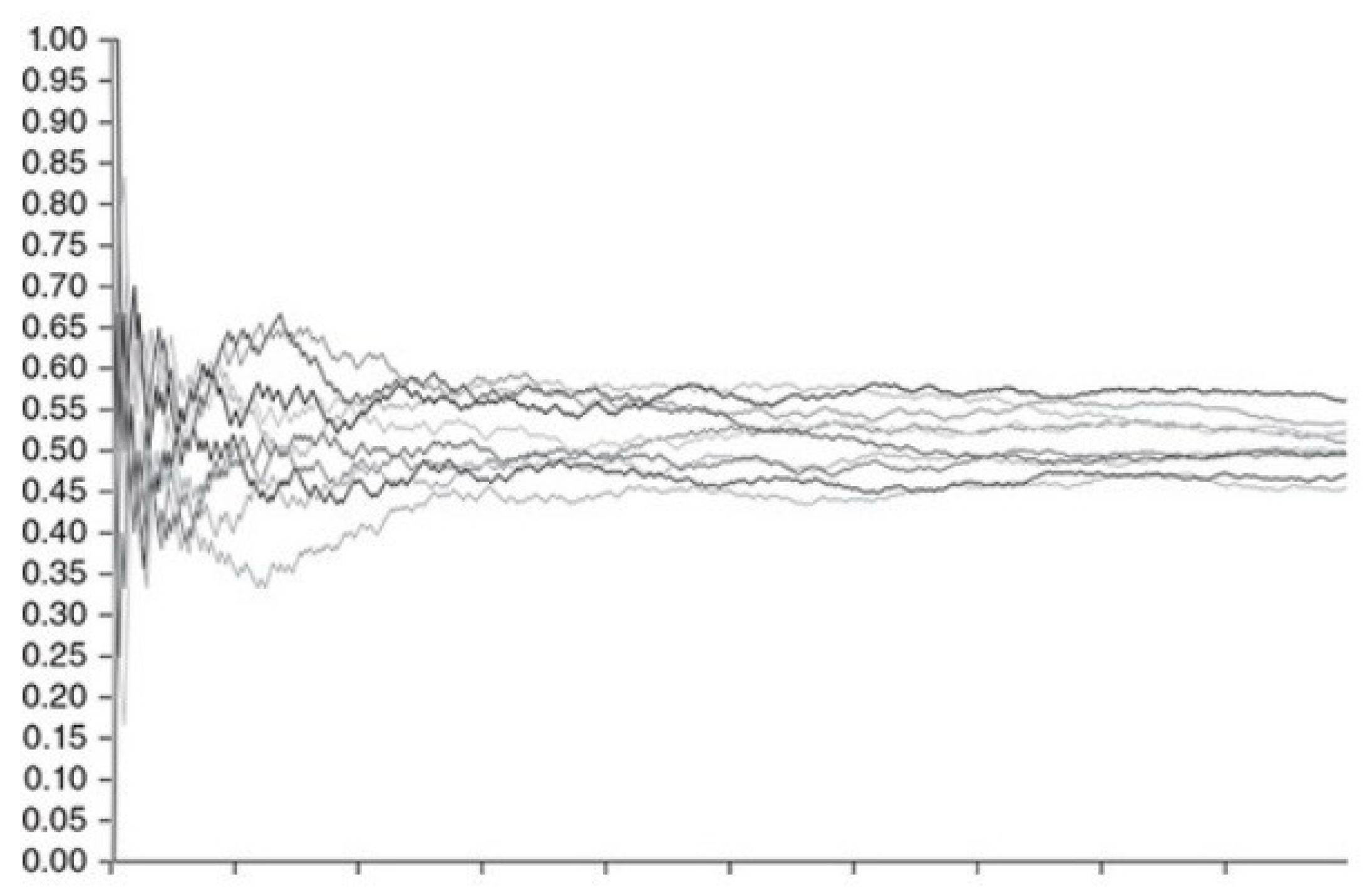
Disclaimer/Publisher’s Note: The statements, opinions and data contained in all publications are solely those of the individual author(s) and contributor(s) and not of MDPI and/or the editor(s). MDPI and/or the editor(s) disclaim responsibility for any injury to people or property resulting from any ideas, methods, instructions or products referred to in the content. |
© 2025 by the authors. Licensee MDPI, Basel, Switzerland. This article is an open access article distributed under the terms and conditions of the Creative Commons Attribution (CC BY) license (http://creativecommons.org/licenses/by/4.0/).
Copyright: This open access article is published under a Creative Commons CC BY 4.0 license, which permit the free download, distribution, and reuse, provided that the author and preprint are cited in any reuse.


