Submitted:
30 June 2025
Posted:
02 July 2025
You are already at the latest version
Abstract
The economics of the energy storage system is constrained by the wind and solar outputs and load demand, so the time scale and representativeness of the dataset are crucial for the optimisation of the system. In order to accurately extract typical operating condition data, this paper adopts the Parzen window estimation method, which is suitable for the characteristics of wind, PV and load data, and the method is able to accurately extracting the typical operating condition data. In this paper, in the process of wind power, photovoltaic and load data analysis and extraction of typical working conditions, the establishment of a reasonable typical time scale to select indicators, in accordance with the three evaluation indexes of the typical time length of 1-7 days to make a separate evaluation of the three indicators of wind power, the three indicators of the optimal typical length of 4 days; photovoltaic indicator 1 optimal typical length of 3 days, indicator 2 and indicator 3 optimal typical length of 2 days; The optimal typical length of time for all three indicators of customer load is 3 days. Then using the game theory combination assignment method, the most realistic typical time scale is 3 days.
Keywords:
energy storage systems
; Parzen window estimation method
; typical operating condition data
; typical time scales
; the game theory combination assignment method
1. Introduction
The problems of grid integration of wind power and solar power systems stem mainly from their intermittent and fluctuating nature. Fluctuations in wind speed and solar irradiance lead to instability in power generation, which poses a challenge to the stable supply of electricity to the grid. Energy storage technology provides a solution by storing energy during excess wind and solar generation and releasing it during peak demand or generation shortfalls, enhancing grid flexibility and reliability. However, the economics of energy storage systems are constrained by the output of wind energy, the output of solar energy and the load demand. The time scales and representativeness of the fundamental datasets made up of wind, solar and load more closely fit the actual scenarios, the size and operating strategy of the energy storage system is more reliable [1]. A control-oriented optimization framework for grid-tied wind-solar-battery hybrid systems has been developed, addressing renewable intermittency challenges through dynamic storage coordination algorithms that enhance energy dispatch precision and grid resilience [2]. Recent advancements in energy storage systems have been comprehensively categorized, with in-depth analyses of their real-world implementations and critical roles in enhancing grid stability through dynamic compensation mechanisms [3]. Research has indicated that a substantial decrease in energy storage costs can have a profound impact on the development of a highly reliable wind power system. This finding offers a crucial viewpoint for the exploration of energy storage economics [4]. The synergistic application of solar/wind energy and advanced water electrolysis methods in hydrogen generation has been extensively analyzed in technical literature, particularly regarding system configurations and efficiency benchmarks [5]. The transition toward decentralized energy systems prioritizes grid integration of solar and wind resources as sustainable alternatives to fossil-fuel plants, ensuring reliable electricity supply during demand surges while optimizing cost-efficiency for end-users through distributed generation architectures [6]. A dynamic optimization framework is introduced to assess how strategically deploying renewables and storage technologies affects grid reliability and cost structures across multiple time horizons [7]. The rapid deployment of grid-tied photovoltaic infrastructure introduces operational complexity to regional power networks, as solar output intermittency driven by meteorological variability poses significant challenges to energy management systems attempting to balance supply-demand equilibrium [8].
In this context, the Parzen window estimation method, due to its non-parametric nature, provides a more flexible solution.
A nonparametric framework has been developed for power system security evaluation, employing kernel-based density estimation to model probabilistic distributions of wind power profiles, generation patterns, and load fluctuations [9]. A novel two-stage thresholding method for image segmentation is proposed, integrating weighted Parzen window and linear programming for efficiency [10]. An architecture for multivariate probability density estimation via the Parzen window approach was proposed. It leverages Parzen window methodology to estimate multivariate probability densities, offering a structured framework for such estimations [11]. A two-phase methodology is introduced for region segmentation: initial seed point generation via kernel-based density estimation, followed by logarithmic clustering for boundary identification; iterative region expansion and contour refinement through probabilistic density modeling of spatial distributions [12]. The Parzen window estimation method is employed to extract features from historical data, deriving distributions of typical weekly wind power, solar power, and load. These distributions are compared with Weibull and Beta distributions. A multi-objective optimization framework, combined with evolutionary algorithms, enhances the sizing and allocation of hybrid wind-solar-storage systems to achieve better economic efficiency under dynamic energy market constraints [13]. A stochastic computational framework is developed for power flow uncertainty quantification, employing kernel-based nonparametric methods to derive probabilistic distributions of grid variables while explicitly modeling interdependencies among wind farms, demand profiles, and electric vehicle charging infrastructures [14]. A novel threshold selection framework for image segmentation is developed by integrating information-theoretic metrics with kernel density estimation, enabling adaptive boundary detection in complex visual datasets [15].
In the process of extracting typical data characteristics of wind power, photovoltaic, and load, known functions (such as normal distribution, Beta distribution, and Weibull distribution) fail to accurately describe the probability distribution. Moreover, some classical probability density functions are unimodal, while the probability density functions of wind power, photovoltaic, and load sample data are mostly multimodal, which directly affects the accuracy of the typical day data. The paper proposes a method using the Parzen window estimation method and a weighted average method to obtain typical data. As a non-parametric estimation method, the Parzen window estimation does not rely on the constraints of the overall probability distribution and does not overly depend on probability parameters, making the model robust. A review of wind speed and wind power prediction methods is presented, focusing on analyzing the characteristics and probability distributions of wind power data, along with the processing of such data by various prediction techniques[16]. A review of data preprocessing and mining methods applied to smart meter data profiling was conducted, offering novel insights for data processing in wind power and photovoltaic datasets[17]. A dimensionality-aware scene analysis framework is developed by integrating manifold learning techniques with adaptive density modeling, enabling robust identification of representative patterns in high-dimensional visual data[18]. An intelligent control framework for hybrid solar-wind energy systems is developed, integrating fuzzy inference mechanisms at critical operational nodes to dynamically optimize renewable resource utilization and maximize power conversion efficiency[19]. A description of the seasonal distribution characteristics of photovoltaic (PV) power generation fluctuations was presented, along with a method for predicting PV power generation uncertainty based on seasonal classification. This approach leverages seasonal patterns to enhance the accuracy of uncertainty predictions in PV power generation[20]. This study evaluates the performance of multiple machine learning algorithms in predicting energy output and power generation for integrated PV/wind systems, leveraging seven meteorological variables identified as critical determinants of renewable energy yield[21].
During the selection of typical time scales, different time scales can influence economic optimization, such as inaccurate energy reserve estimates, neglecting long-term trends, failing to consider multiple system operating scenarios, and declining reliability. Therefore, this paper establishes reasonable indicators for typical time scale selection and uses a game theory-based combination weighting method to obtain the most practical typical time scale.
This paper first establishes a Parzen window model and extracts typical data characteristics of wind power, photovoltaic, and user demand. Then, it develops evaluation indicators for time scale selection, and finally uses the game theory-based combination weighting method to determine the optimal time scale.
2. Parzen Window Estimation Method
The main methods for extracting typical data curves are parametric and non-parametric estimation methods. For the uncertainty characteristics of wind/photovoltaic, the Parzen window estimation method (non-parametric estimation method) will be more applicable.
The expression for the Parzen window estimation method is as follows[22]:
In (1), f(x) represents the probability density function; K(x) for the window function;h is the bandwidth (smoothing parameter);N is the total number of sample data;Xi for the given sample. Parzen Window functions commonly used in window estimation methods include Gaussian Functions, Triangle functions and Epanechniko function. Their expressions are respectively:
In (2), The value domain of x in the trigonometric and Epanechniko functions is 0-1, which needs to be normalised if used for wind speed/solar irradiance and user load estimation. and the three window functions have little effect on Parzen window estimation. A major influence on the Parzen window estimation method is the bandwidth h. The effect of different bandwidths on the results for wind speed, for example, is shown in Figure 1. The bandwidth h is in the interval of [0.01,10], and the bandwidth with the smallest mean square error is selected as the best bandwidth by matching the optimisation in steps of 0.01.
3. Extract Typical Data Features
3.1. Extraction of Typical Data Features for Wind Power
Extracting typical data features for wind power includes three steps: firstly, Wind power data pretreatment. Removing outliers, filling in missing values, and data smoothing to ensure the quality and reliability of the data used. Secondly, create a probability density curve. This is done through Parzen window estimation method and this method helps to establish the trend of power generation at different wind speeds. Thirdly, verify the theoretical output curve of the turbine. The established wind speed probability density curves need to be validated against the theoretical power curves of the turbines to assess the accuracy of the model and provide reference for subsequent work. Through this series of steps, the researcher can establish the typical data wind output power curve model, which is of significant value for optimising the design and operation of wind farms.
In this paper, a region in Inner Mongolia Autonomous Region, China, was selected to(N 39°61′、E 109°78′)The actual wind speed data of a weather station from 1 January 2020 to 31 December 2020 were analysed with a sampling interval of fifteen minutes as shown in Figure 2.
(1) Wind power data pretreatment
The wind speed range probability plot is shown in Figure 3. Based on the above data characteristics Goldwind AW82/1500 wind turbine is selected and its parameters are shown in Table 1. As shown in Figure 4, Goldwind AW82/1500 wind turbine can be used for 92.08 % of the total number of working hours, of which 22.92 % of the total number of working hours are in full state.
The expression of the Goldwind AW82/1500 wind turbine is:
In (3), v、vr、vcut-in and vcut-out represent the actual wind speed, rated wind speed, cut-in wind speed and cut-out wind speed of the wind turbine, respectively. Pr Indicates rated power. The relationship between the data is shown in Figure 5, and the red line is the theoretical output power curve of the wind turbine.
Taking the typical data time selection of 24 hours as an example, the modeling process of the Parzen window estimation method for the typical power curve extraction for the minutes 0:00-0:15 is as follows:
(1) According to the IEC61400-12-1 standard [23], valid wind speed data from available samples were counted from 0:00 to 0:15 every day.
(2) Use Bin's method for interval delineation to calculate the probability density of each interval using an integer multiple of 0.5 m/s as the center point.
(3) Summarize all probability densities to create a Parzen window probability distribution curve.
The optimal Weibull probability density distribution curve [24] was obtained using the method described in reference [25]. Figure 6 shows the probability distributions of wind speeds from 0:00 to 0:15 minutes obtained by different methods. In this time period, the optimal bandwidth is 0.3209 and the optimal shape and scale parameters in the Weibull probability distribution function are 2.1066 and 8.7573, respectively.
In order to compare the closeness of the Parzen probability , Weibull probability curves to the wind speed probability, respectively, the following Root Mean Squared Error (RMSE) formula can be used:
In (4), n is the total number of data points, y 1, i is the ith Standard value, y 2, i is the ith value to be compared.
The root mean square error was calculated to be 0.001879 for Parzen probability and wind speed probability and 0.005260 for Weibull probability and wind speed probability. In Figure 6 the Weibull probability distribution differs from the probability histogram, especially at wind speeds between 10 m/s-15 m/s. The Parzen window estimation method is more in line with the true distribution of the data and has a higher degree of accuracy, which provides an initial validation of the reliability of the Parzen probability distribution.
3.2. Extracting Typical Data Characteristics of PV
In this paper, the actual solar irradiance data from a meteorological station in a region of Inner Mongolia Autonomous Region, China (N 39°61′, E 109°78′) from January 1, 2020 to December 31, 2020 are selected for analysis with a sampling interval of fifteen minutes. As shown in Figure 7, the solar irradiance observed at the weather station throughout the year is demonstrated.
As shown in Figure 8, 45.91 % of the total annual data observed by the weather stations had solar irradiance equal to 0, 4.19 % had solar irradiance greater than 1000 W/m2. Solar irradiance greater than 0 and less than 200 W/m2 accounted for 19.22 % of the total. Solar irradiance in the range of 200 W/m2 – 1000 W/m2 accounted for 30.68 % of the total. The annual average solar irradiance in the data observed at the meteorological stations was 237.07 W/m2. But when selecting PV panels, it is not necessary to consider the period of time when the solar irradiance is 0. If this situation is not taken into account, the annual average solar irradiance is 529.07 W/m2.
In a photovoltaic power plant, the theoretical expression between solar irradiance and the output power of photovoltaic power generation is:
In (5), PPV is the output power of the photovoltaic plant (in W),I is the solar irradiance (in W/m2),A is the area of the photovoltaic panel (in m2),ηPV For the photovoltaic panel conversion efficiency, the current domestic mainstream photovoltaic panel conversion efficiency between 15 %-40 %, the photovoltaic panel conversion efficiency selection of 30 %.
The annual solar irradiance is converted into the output power of the PV plant per unit area, and its distribution is shown in Figure 8. The PV panel model CY-TJ 250 is selected and its parameters are shown in Table 2. According to the above data features CY-TJ 250, without counting the moments when the output power is 0, the distribution of the PV panel output power is shown in Figure 9, the PV panel full working hours accounted for 7.75 % of the total number of hours, and the output power is less than 100W hours accounted for 51.60 % of the total number of hours, which further verifies the scientific nature of the selected PV panel model.
Taking the typical data time selection of 24 hours as an example, the typical power curve is extracted for the minutes 10:00-10:15, and the modeling process of the Parzen window estimation method is as follows:
(1) Normalize the data and consider the solar irradiance exceeding 1000 W/m2 as 1000 W/m2.
(2) Use Bin's method to divide the intervals, and use 0.1 W/m2 as an integer multiple of 0.1 W/m2 as the center point, and calculate the probability density of each interval.
(3) Summarize all the probability densities to build the Parzen window probability distribution curve.
The best Beta probability density distribution curve was obtained using the method described in reference [26]. Figure 10 shows the probability distribution of solar irradiance for the 10:00-10:15 minutes obtained by different methods. The optimal bandwidth is 0.0273 for this time period.
When examining the probability distribution characteristics of PV data, Beta distribution curves are often used to model the knowledge accumulation of the data. As shown in Figure 10, the shape parameter of the Beta distribution determines the type of distribution it can represent, and for complex PV data distributions, it is still not possible to accurately capture all the peaks, resulting in its inability to fully reflect the overall distribution trend.
In contrast to the Beta distribution, the Parzen window method provides a nonparametric means of estimating probability densities that makes no assumptions about the form of the distribution of the data. A more flexible density estimate is constructed by accumulating weights in the vicinity of sample points through a sliding window. In Figure 10, the root-mean-square error of Parzen probability and wind speed probability is calculated to be 0.020376, and the root-mean-square error of Weibull probability and wind speed probability is 0.039799, and the Parzen probability distribution is more effective in fitting the PV data.This method is not limited by the shape of a particular distribution, and thus can better accommodate the phenomenon of multiple peaks in the data, exhibiting a smaller overall error than the Beta distribution.
In summary, although the Beta probability distribution is widely used in various types of data analysis due to its computational simplicity and solid theoretical foundation, the Parzen window method clearly provides a more reasonable and effective probability density estimation for photovoltaic data with complex distributional characteristics.
3.3. Extract Typical Data Features of User Requirements
In this paper, the actual customer load data from January 1, 2020 to December 31, 2020 in a region of Inner Mongolia Autonomous Region of China (N 39°61′, E 109°78′) is selected for analysis, with a sampling interval of fifteen minutes, as shown in Figure 11.
Taking the typical data time selection of 24 hours as an example, typical power curves were extracted for the minutes 10:00-10:15, and the modeling procedure for the Parzen window estimation method was as follows:
(1) Normalize the data;
(2) Use Bin's method to partition the intervals, using an integer multiple of 0.1 MW as the center point, and calculate the probability density of each interval.
(3) Summarize all probability densities to create a Parzen window probability distribution curve.
Figure 12 shows the probability distribution profile of the customer load demand from 00:00 to 00:15 minutes obtained using the Parzen window estimation method. The optimal bandwidth is 0.02 during this time period.
4. Typical Time Scale Selection
In the process of analyzing wind power data, photovoltaic power generation data and customer load data and extracting typical working conditions, the selection of typical time length is a decisive factor. It directly affects the type of wind, photovoltaic, load variation characteristics and operating conditions that we are able to identify.
As shown in Figure 13, the typical time lengths were selected as 1 day, 4 days and 7 days, and using the typical operating condition curves obtained for wind power output. Because the cube of wind speed is proportional to the wind power output, resulting in large differences in the wind power output curves obtained for different typical time lengths, which demonstrates the importance of the typical time length selection.
As shown in Figure 14, typical time lengths of 1 day, 4 days and 7 days were selected and the typical operating conditions curves of the obtained photovoltaic outputs were utilized, from which it can be seen that there are large differences in the peak areas of the two typical operating conditions curves (with typical time lengths of 1 day and 7 days) in the interval from 0 to 24 hours. And in the interval from 24 to 48 hours, the two typical operating conditions curves (with typical time lengths of 4 days and 7 days), there is a large difference in the peak region, which also proves the importance of the selection of the typical time length.
As shown in Figure 15, the typical time lengths of 1 day, 4 days and 7 days were selected and the typical operating conditions curves of the obtained photovoltaic outputs were utilized, from which it can be seen that there are differences in the peak areas of the three typical operating conditions curves in the interval from 0 to 24 hours. In particular, there are large differences in the peaks between the operating conditions curves when the typical time length is 1 day and the curves for the other two days. In the interval from 72 to 96 hours, both the peak region and the peak-to-valley region of the two typical operating condition curves (with typical time lengths of 4 and 7 days) differed considerably. This also demonstrates the importance of the typical length of time chosen.
4.1. Extract Typical Data Features of User Requirements
The purpose of creating statistical indicators is to quantify the difference between a typical day relative to the raw data in the aggregate and across time periods. In particular, the deviation of the total load power for the year represents the relative error of the total load power on a typical day, calculated by weighting, to the total load power of the original data, as follows [27]:
In (6), Cd Indicates the sum of typical data selected;Cyear Indicates one year of total data;year Equals 365;d Indicates the number of days selected. The smaller the deviation of the resource throughout the year, the more accurate the data selected for the typical time.
Pearson Correlation Coefficient describes well the correlation of 2 sets of data, let there exist 2 arrays of X、Y,When r>0, then the positive correlation between the 2 sets of data is stronger, and when r<0, then the negative correlation between the 2 sets of data is stronger.
In (7), m is the number of elements in the array. The average of the absolute values of the correlation coefficients between the typical time data and all the data is used as indicator 2, which is calculated as follows:
The larger the indicator 2, the stronger the correlation between the typical time data and the original data, and the better the selection of typical data. The data bias represents the relative error of the data for the same time period over all typical days as compared to the data for the same time period of the historical data, and indicator 3 is the average of the deviations of the data over all time periods, as follows:
In (9), D and D0 are the set of all dates for typical and original data, respectively; Pi,t is the data value of date d at moment t. The smaller the indicator 3, the better the selection of typical data.
Strictly in accordance with the above three evaluation indexes to make a separate evaluation of the typical time length of 1-7 days, the results are shown in Table 3. The optimal typical length of time for all three indicators of wind power is 4 days; the optimal typical length of time for photovoltaic indicator 1 is 3 days, and the optimal typical length of time for indicators 2 and 3 is 2 days; the optimal typical length of time for all three indicators of customer load is 3 days. In order to select the optimal typical time length, need to develop a harmonized weighting scheme.
4.2. Evaluation Methodology
Ordinal Relationship Method [28] (ORA) is a subjective assignment method, with the advantages of small amount of calculation, without the need to construct judgment matrix, and its general steps are as follows:
(1) Determine the ordinal relationship of the indicators; based on importance and expert recommendations, establish the ranking order among the three indicators.
(2) The expression of the judgment of the degree of importance between the two neighboring indexes is:
In (10): k takes values of 2 and 3, X represents the value of the evaluation indicator, and Rk denotes the importance between the k-th evaluation indicator and the k-1-th evaluation indicator.
(3) The weight coefficient of the k-th evaluation indicator is:
The weight coefficient of the k-1-th evaluation indicator is:
Based on the above process, the subjective weights of the indicators are shown in Table 4. Because in the source-load-storage system the generation side (source) is wind and solar energy, and the load side (load) is the customer load, the load share is 0.5; the share of wind and solar energy is 80 % + 20 %[29], so the share of wind energy is 0.4 and the share of solar energy is 0.1.
Entropy Weight Method is an objective assignment method [30] with the following general steps:
(1) The data Xm×n are quantized with the expression:
In (14), zij is the standardized value of the j-th evaluation indicator in the i-th evaluation scheme.
(2) The weight of the j-th evaluation indicator in the i-th evaluation program is:
(3) The entropy value of the j-th evaluation indicator is:
(4) The weight of the j-th evaluation indicator is:
Based on the above process, the objective weights of the indicators are shown in Table 5.
The two sides of the game are the subjective weight W1 obtained by ORA and the objective weight W2 obtained by Entropy Weight Method, whose expressions are[31]:
The combination weight expression is:
In (20), λ is the linear combination coefficient. With the sum of the minimum deviations between the combined weights and the individual weights as the objective function, the optimal linear combination coefficient is solved, and its constraint condition expression is:
In (21): λ1 and λ2 are both greater than or equal to 0, and their sum equals 1. From the principle of differentiation, the model is also required to satisfy the first-order derivative condition, which is expressed as:
Normalizing λ yields the optimal linear combination coefficients, which are expressed as:
The expression for the optimal combination of weights for the evaluation indicators is:
In summary, the optimal linear scaling factors are found to be 0.3854 and 0.6146 respectively. The final combination weights are obtained by calculation as shown in Table 6.
It was obtained that the typical time length choice of 3 days best characterized the original data and had the best overall correlation with the original data. The typical data feature extraction method is strictly implemented to obtain the typical operating condition curves of wind power, PV, and customer loads as shown in Figure 16.
From the figure, it can be seen that the average wind power generation is 0.67 MW. At this power level, the wind speed is 8.48 m/s, which is only 0.23 m/s higher than the actual annual average wind speed, with an error of 2.7 %. This indirectly demonstrates the feasibility of selecting typical wind power data. Ignoring the moments when the power generation is 0, the average photovoltaic power generation is 74.05 W/m². At this power level, the solar irradiance is 246.83 W/m², which is only 9.76 W/m² higher than the actual annual average solar irradiance, with an error of 3.94 %. This indirectly demonstrates the feasibility of selecting typical photovoltaic data. The average user load power is 64.83 MW, which is only 2.24 MW higher than the actual annual average electricity load, with an error of 3.45 %. This indirectly demonstrates the feasibility of selecting typical user load data.
5. Conclusions
This paper analyzes the uncertainty of wind power generation, solar power generation, and user load variations. Through comparative analysis, when dealing with the uncertainty of wind power generation and user load under typical operating conditions, the Parzen window estimation method (a non-parametric estimation method) is more consistent with the true distribution of the data and offers higher accuracy during the process of extracting probability distribution curves. Since the output curves differ significantly when the typical time lengths are set to 1 day, 4 days, and 7 days, the best indicator weight is finally calculated, and it is determined that the typical operating condition curve most closely aligns with the actual situation when the typical time scale is 3 days.
Institutional Review Board Statement
Not applicable. Our study did not involve human or animal subjects.
Informed Consent Statement
Not applicable. Our study did not include any individual person’s data, images, or videos. Data available on request from the authors.
Data Availability Statement
Not applicable. This manuscript does not report data generation or analysis.
Conflicts of Interest
All the authors certify that they have no affiliations with or involvement in any organization or entity with any financial interest or nonfinancial interest in the subject matter or materials discussed in this manuscript
Author Contributions
All authors reviewed the manuscript.
Funding
The research work presented in this paper is financially supported by the National Natural Science Foundation of China (Grant 52465008), the Natural Science Foundation of Inner Mongolia (Grant 2024QN05042). The authors also acknowledge support from the Basic Scientific Research Fund Project of Universities Directly Under the Jurisdiction of the Inner Mongolia Autonomous Region through grants 2024QNJS075 and 2024QNJS012.
Acknowledgments
not applicable.
References
- UAN Tiejiang, CHE Yong, SUN Yiqian, et al. Optimized proportion of energy storage capacity in wind-storage system based on timing simulation and GA algorithm . High Voltage Engineering,2017 43 (7 ) : 2122-2130.
- Zhu R, Zhao AL, Wang GC, Xia X, Yang Y. An Energy Storage Performance Improvement Model for Grid-Connected Wind-Solar Hybrid Energy Storage System. Computational Intelligence and Neuroscience. 2020;2020(1):8887227. [CrossRef]
- Ding Z, Bu W, Xu R, et al. Application of Energy Storage Technology in Photovoltaic Power Generation System[C]//8th International Conference on Management and Computer Science (ICMCS 2018). Atlantis Press, 2018: 463-466.
- Tong F, Yuan M, Lewis NS, Davis SJ, Caldeira K. Effects of deep reductions in energy storage costs on highly reliable wind and solar electricity systems. Iscience. 2020 Sep 25;23(9). [CrossRef]
- Nasser M, Megahed TF, Ookawara S, Hassan H. A review of water electrolysis–based systems for hydrogen production using hybrid/solar/wind energy systems. Environmental Science and Pollution Research. 2022 Dec;29(58):86994-7018. [CrossRef]
- Ahmed M M R, Mirsaeidi S, Koondhar M A, et al. Mitigating Uncertainty Problems of Renewable Energy Resources Through Efficient Integration of Hybrid Solar PV/Wind Systems Into Power Networks[J]. IEEE Access, 2024, 12: 30311-30328. [CrossRef]
- Lamadrid AJ. Optimal use of energy storage systems with renewable energy sources. International Journal of Electrical Power & Energy Systems. 2015 Oct 1;71:101-11. [CrossRef]
- Wang F, Zhen Z, Mi Z, Sun H, Su S, Yang G. Solar irradiance feature extraction and support vector machines based weather status pattern recognition model for short-term photovoltaic power forecasting. Energy and Buildings. 2015 Jan 1;86:427-38. [CrossRef]
- Ul Hassan R, Yan J, Liu Y. Security risk assessment of wind integrated power system using Parzen window density estimation. Electrical Engineering. 2022 Aug;104(4):1997-2008.
- Xiong F, Zhang Z, Ling Y, Zhang J. Image thresholding segmentation based on weighted Parzen-window and linear programming techniques. Scientific Reports. 2022 Aug 10;12(1):13635. [CrossRef]
- Stanković D, Draganić A, Lekić N, Ioana C, Orović I. An architecture for Parzen-based multivariate probability density estimation. In2024 32nd Telecommunications Forum (TELFOR) 2024 Nov 26 (pp. 1-4). IEEE.
- de Souza Rebouças E, De Medeiros FN, Marques RC, Chagas JV, Guimarães MT, Santos LO, Medeiros AG, Peixoto SA. Level set approach based on Parzen Window and floor of log for edge computing object segmentation in digital images. Applied Soft Computing. 2021 Jul 1;105:107273. [CrossRef]
- Yu Q, Gao S, Sun G, Qin R. Optimization of wind and solar energy storage system capacity configuration based on the Parzen window estimation method. Journal of Renewable and Sustainable Energy. 2023 Nov 1;15(6). [CrossRef]
- Rouhani M, Mohammadi M, Kargarian A. Parzen window density estimator-based probabilistic power flow with correlated uncertainties. IEEE Transactions on Sustainable Energy. 2016 Mar 15;7(3):1170-81. [CrossRef]
- Xiong F, Zhang J, Ling Y, Zhang Z. A novel image thresholding method combining entropy with Parzen window estimation. The Computer Journal. 2022 Aug;65(8):2231-44. [CrossRef]
- Wang Y, Zou R, Liu F, Zhang L, Liu Q. A review of wind speed and wind power forecasting with deep neural networks. Applied energy. 2021 Dec 15;304:117766. [CrossRef]
- Dahunsi FM, Olawumi AE, Ale DT, Sarumi OA. A systematic review of data pre-processing methods and unsupervised mining methods used in profiling smart meter data. AIMS Electronics and Electrical Engineering. 2021;5(4):284-314. [CrossRef]
- Wang X, Zhong F, Xu Y, et al. Extraction and Joint Method of PV–Load Typical Scenes Considering Temporal and Spatial Distribution Characteristics[J]. Energies, 2023, 16(18): 6458. [CrossRef]
- Balakishan P, Chidambaram IA, Manikandan M. Smart fuzzy control based hybrid PV-wind energy generation system. Materials Today: Proceedings. 2023 Jan 1;80:2929-36. [CrossRef]
- Shi M, Yin R, Wang Y, Li D, Han Y, Yin W. Photovoltaic power interval forecasting method based on kernel density estimation algorithm. InIOP Conference Series: Earth and Environmental Science 2020 Dec 1 (Vol. 615, No. 1, p. 012062). IOP Publishing.
- Qadir Z, Khan SI, Khalaji E, Munawar HS, Al-Turjman F, Mahmud MP, Kouzani AZ, Le K. Predicting the energy output of hybrid PV–wind renewable energy system using feature selection technique for smart grids. Energy Reports. 2021 Nov 1;7:8465-75. [CrossRef]
- Hassan, R.U.; Yan, J.; Liu, Y. Security risk assessment of wind integrated power system using Parzen window density estimation. Electrical Engineering. 2022, 104, 1–12. [CrossRef]
- IEC 61400-12-1-2017, Wind turbines Generator Systems-Part 12-1: Power performance measurements of electricity producing wind turbines[S].
- A.K. Azad, et al., Analysis of wind energy conversion system using Weibull distribution, Procedia Eng. 90 (2014) 725–732. [CrossRef]
- Chen Haisheng, Li Hong, Xu Yujie, et al. Research Progress of Energy Storage Technologies in China in 2022[J]. Energy Storage Science and Technology (in Chinese), 2023, 12(05): 1516-1552.
- JANI V, ABDI H. Optimal allocation of energy storage systems considering wind power uncertainty[J]. Journal of Energy Storage, 2018, 20: 244-253. [CrossRef]
- Tang Junxi, Cao Huazhen, Gao Chong, et al. A User Load Curve Analysis Method Based on Time Series Data Mining[J]. Power System Protection and Control (in Chinese), 2021, 49(05): 140-148.
- Fang Guohua, Ye Xiaojing, Yao Huaizhu, et al. Evaluation of Rural River Ecological Status Based on Fuzzy Matter-element Method[J]. China Rural Water and Hydropower (in Chinese), 2022(4): 80-84.
- Qihui Yu, Shengyu Gao, Guoxin Sun et al. Optimization of wind and solar energy storage system capacity configuration based on the Parzen window estimation method. Journal of Renewable and Sustainable Energy.2023,15(6):064103. [CrossRef]
- Zhao Shuqiang, Tang Shanfa. Comprehensive Evaluation of Power Transmission Network Planning Schemes Based on Improved Analytic Hierarchy Process, CRITIC Method and Technique for Order Preference by Similarity to an Ideal Solution[J]. Electric Power Automation Equipment (in Chinese), 2019, 39(3): 143-148, 162.
- LI Hao,GAO Liang,LI Peigen.Topology optimization of structures under multiple loading cases with a new compliance-volume product[J].Engineering Optimization,2014,46(6):725-744.
Figure 1.
Probability density curves for different bandwidths.
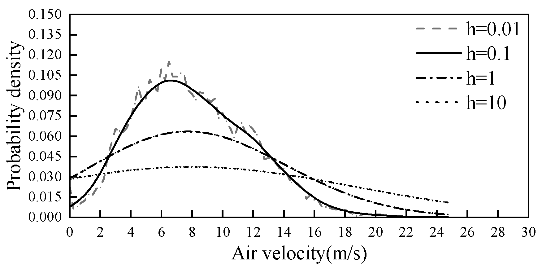
Figure 2.
Real-time wind speed at wind farms.
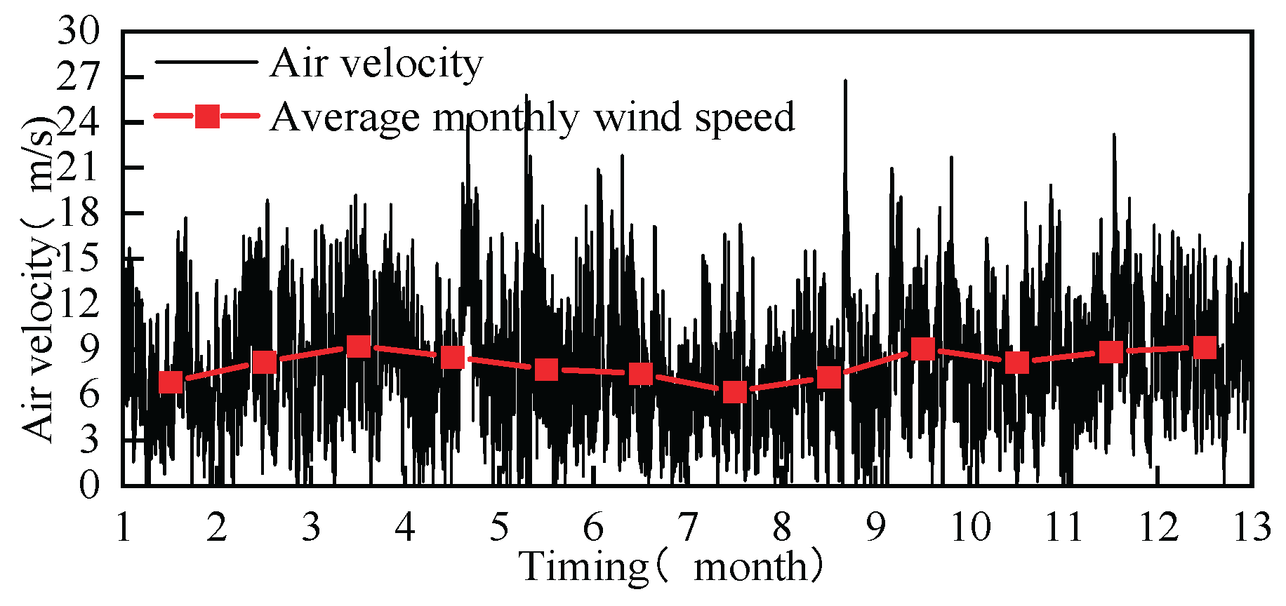
Figure 3.
Probability chart of wind speed rang.
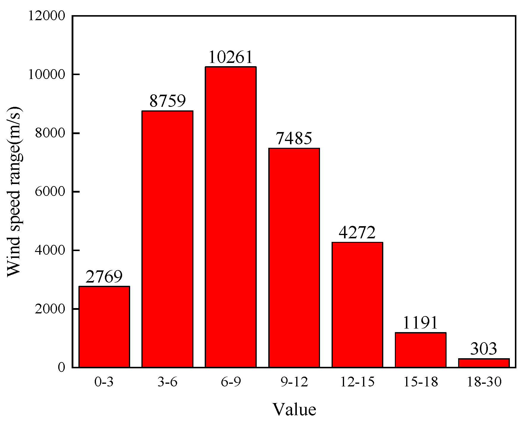
Figure 4.
Probability plot of operating range Goldwind AW82/1500 wind turbine.
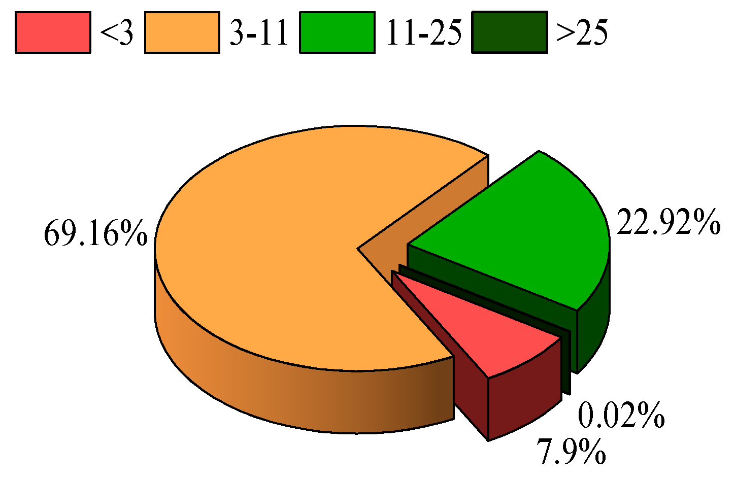
Figure 5.
Wind turbine output power curve.
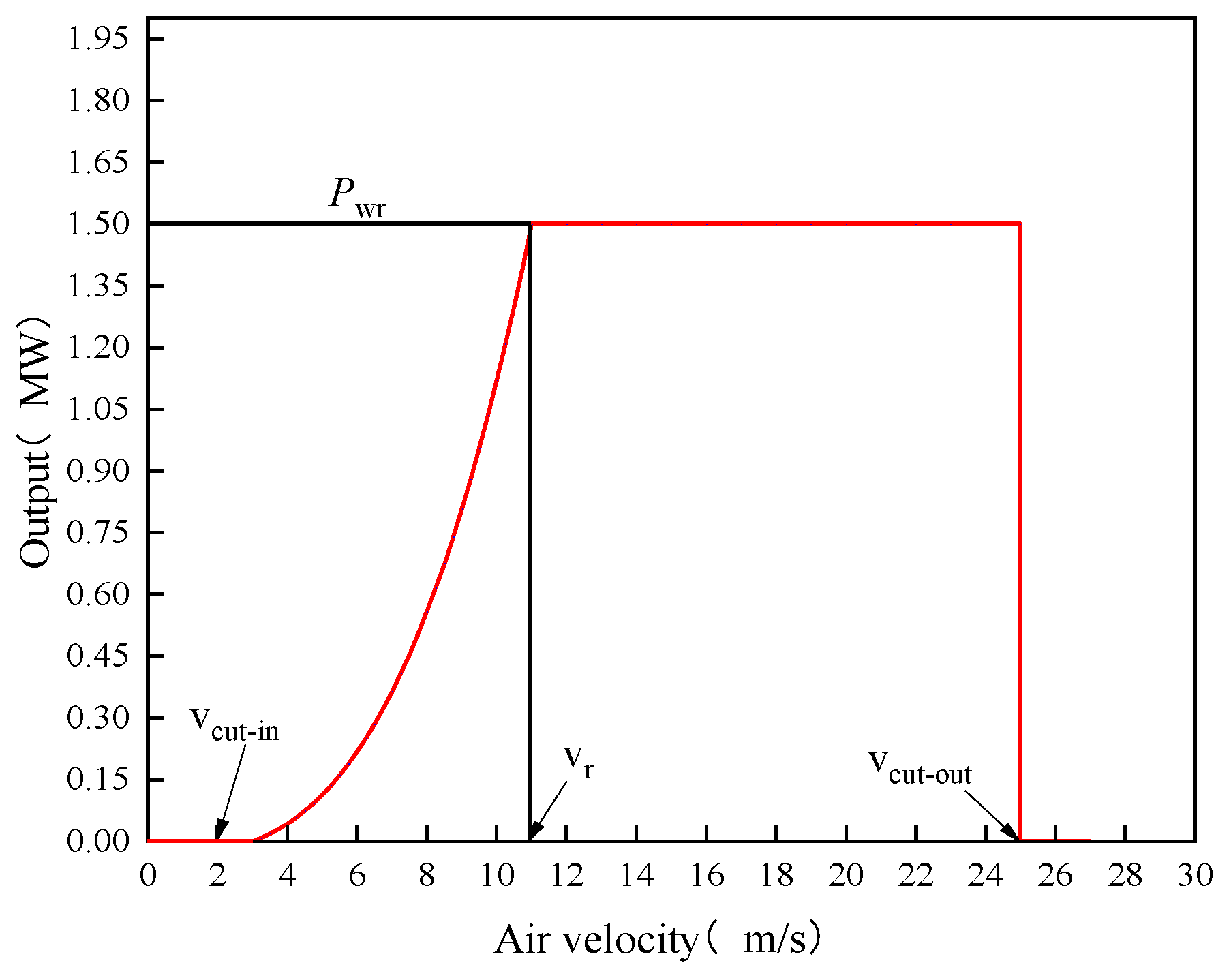
Figure 6.
Probability plot of wind speed distribution (00:00-00:15).
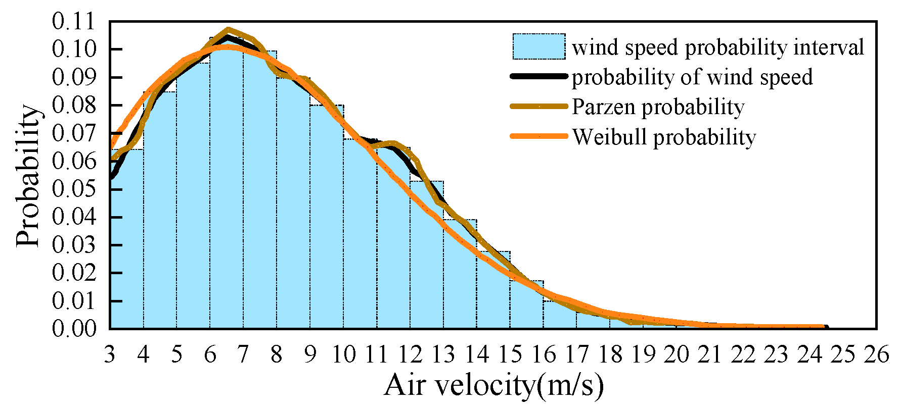
Figure 7.
Real-time solar energy of photovoltaic power plants.
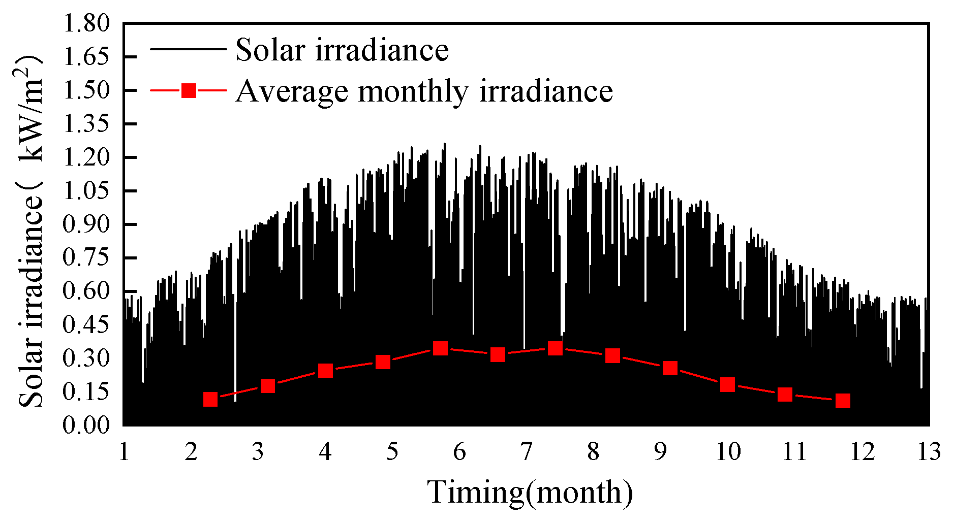
Figure 8.
Probability plot of wind speed ranges.
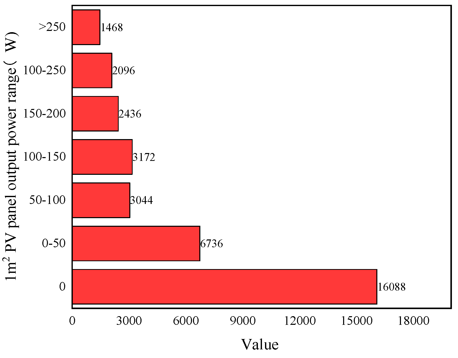
Figure 9.
Probability plot of the working interval of CY-TJ 250.
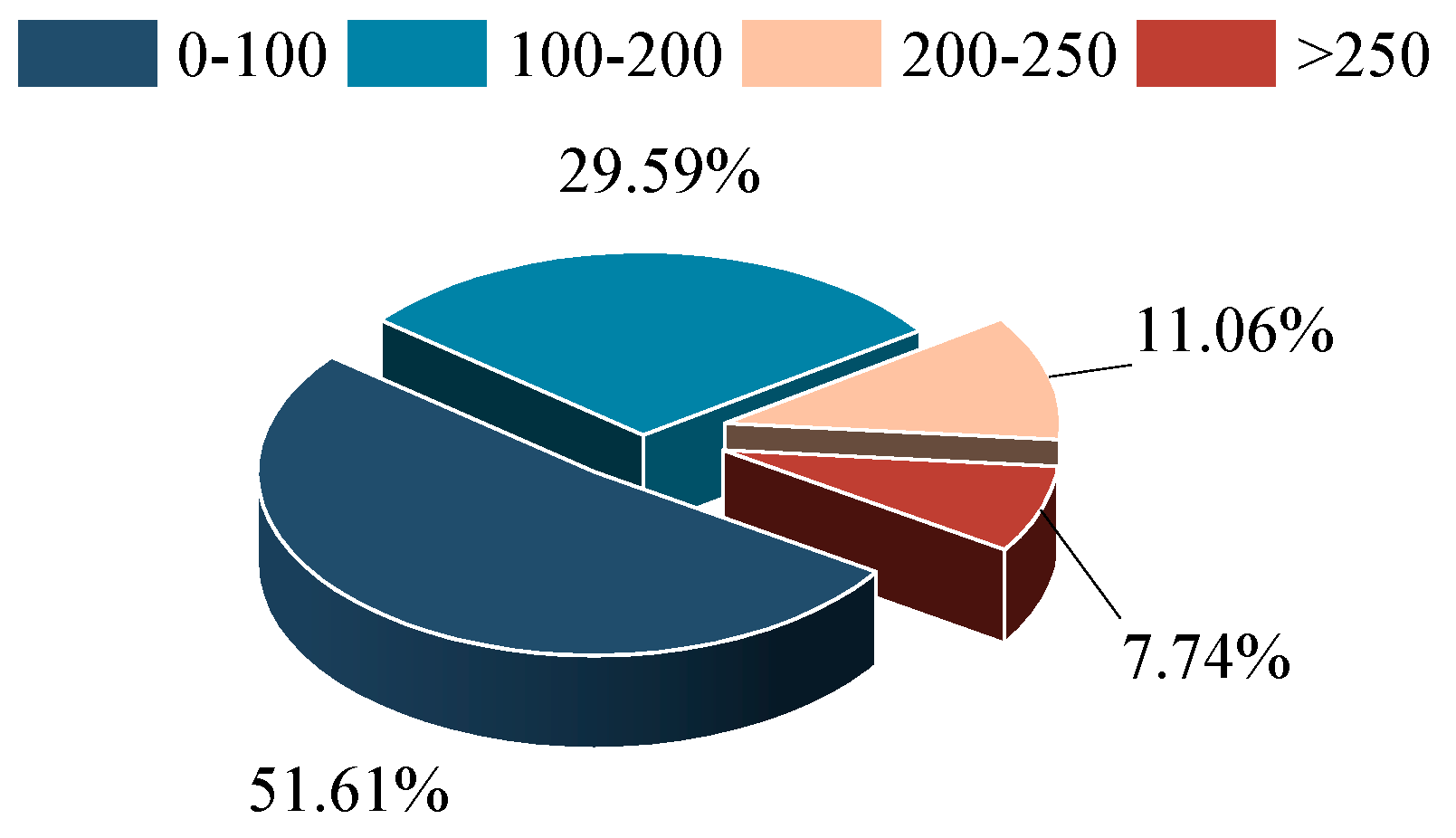
Figure 10.
Standardized solar irradiance distribution probability chart(10:00-10:15).
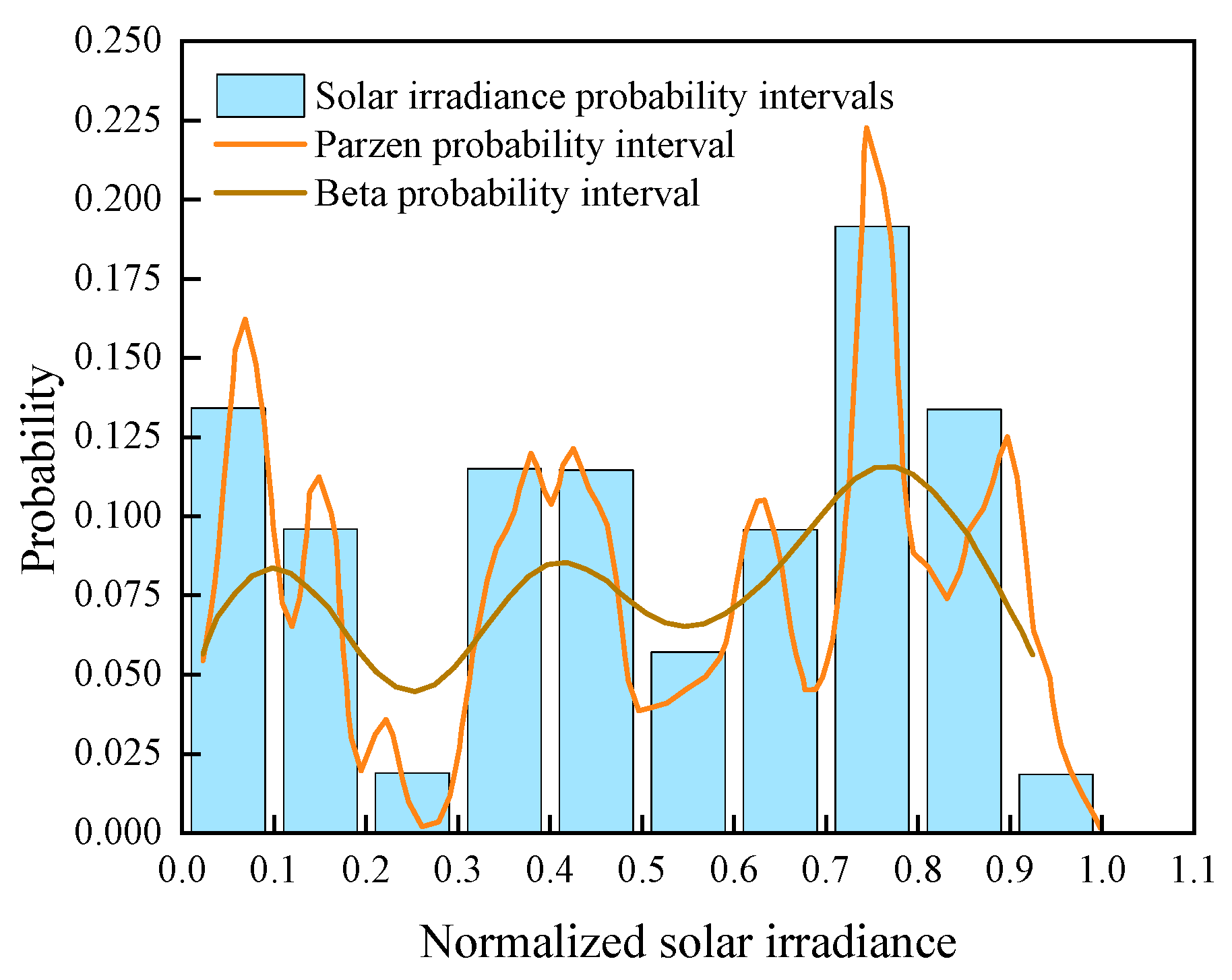
Figure 11.
Real-time load demand.
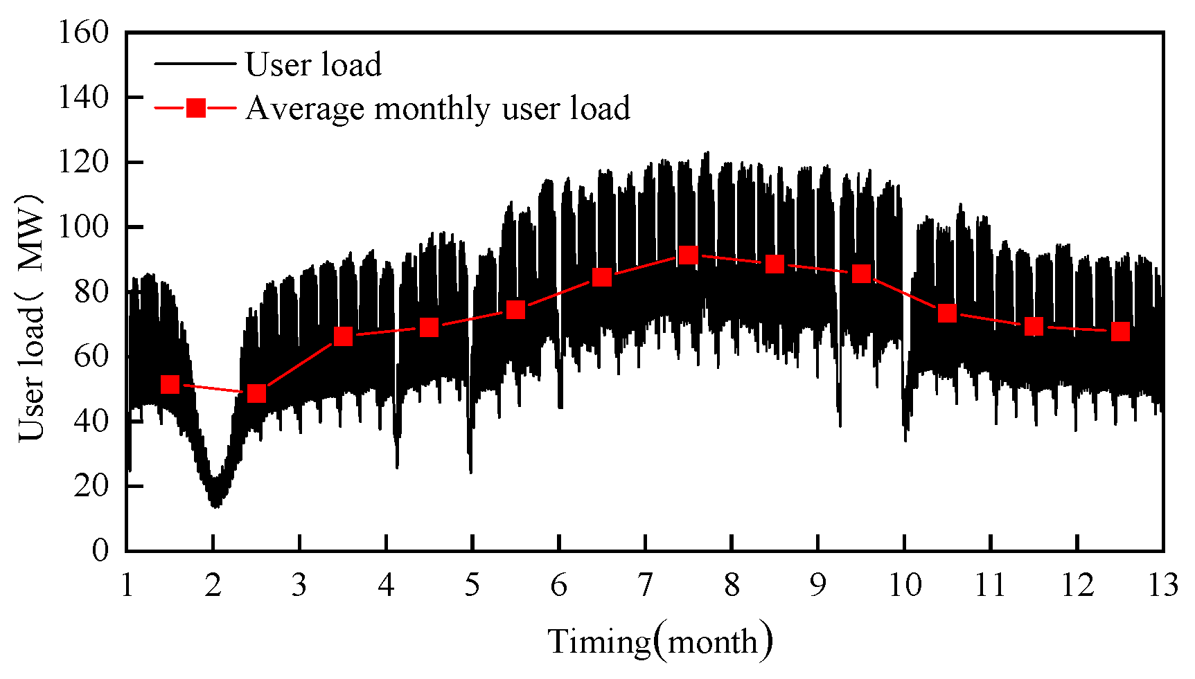
Figure 12.
Probability distribution plot of customer load demand (00:00-00:15).
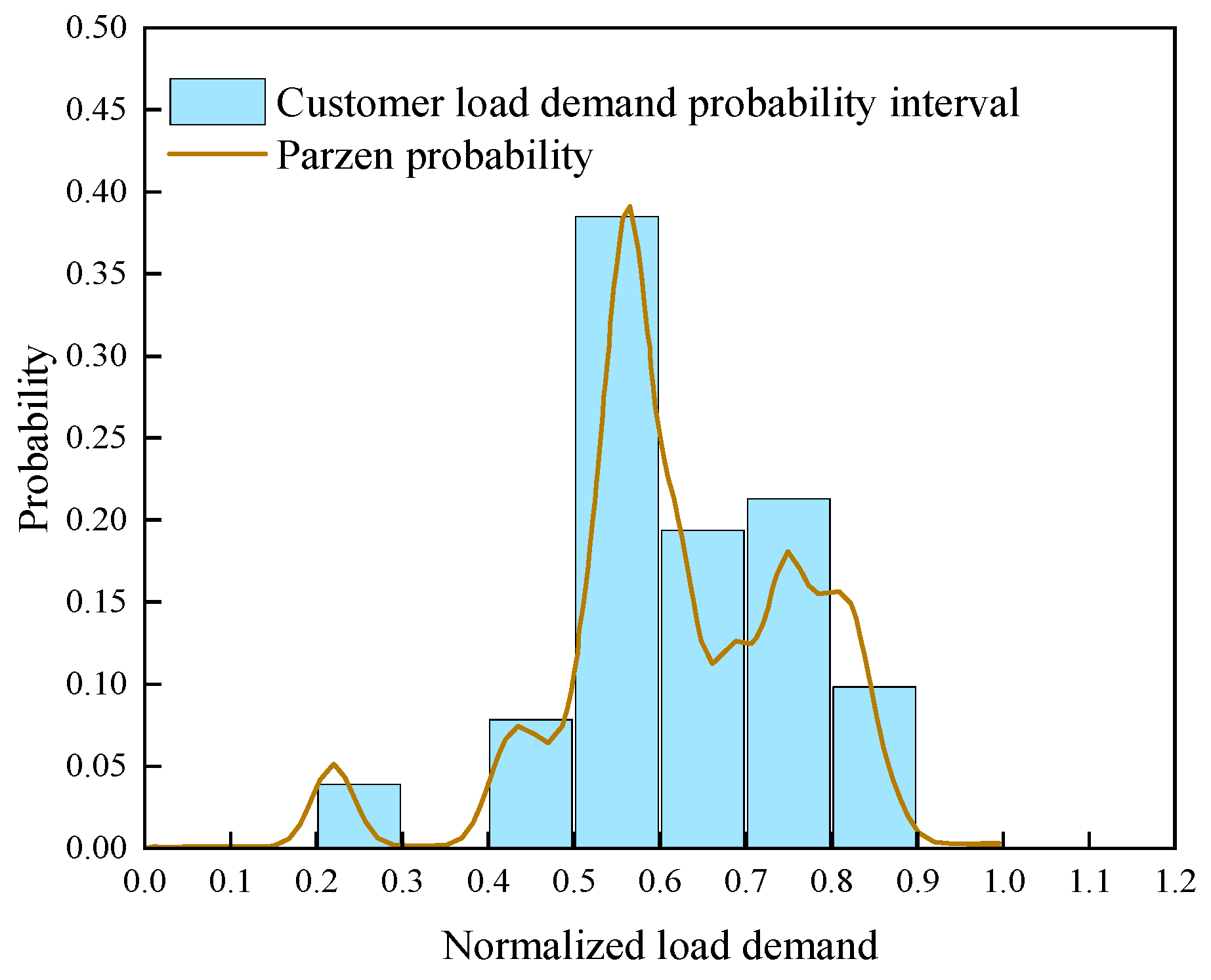
Figure 13.
Comparison of typical time scales for wind power.
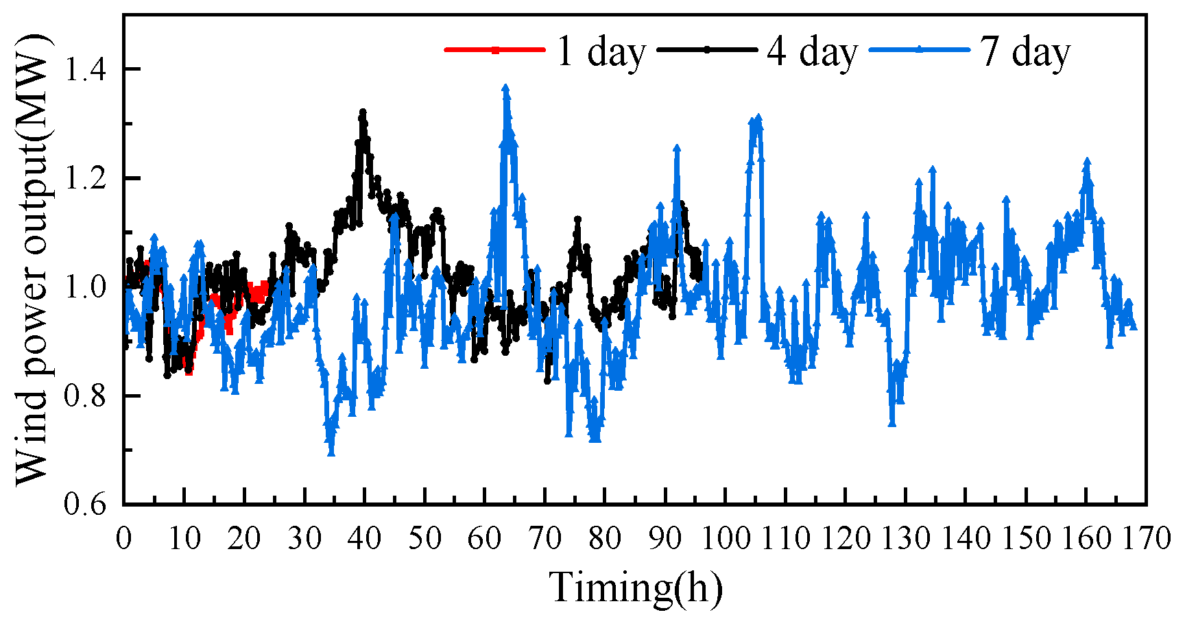
Figure 14.
Comparison of typical time scales for photovoltaic.
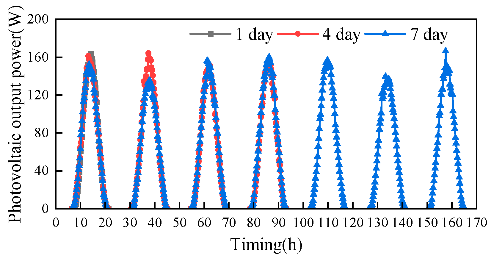
Figure 15.
Comparison of typical time scales of load.
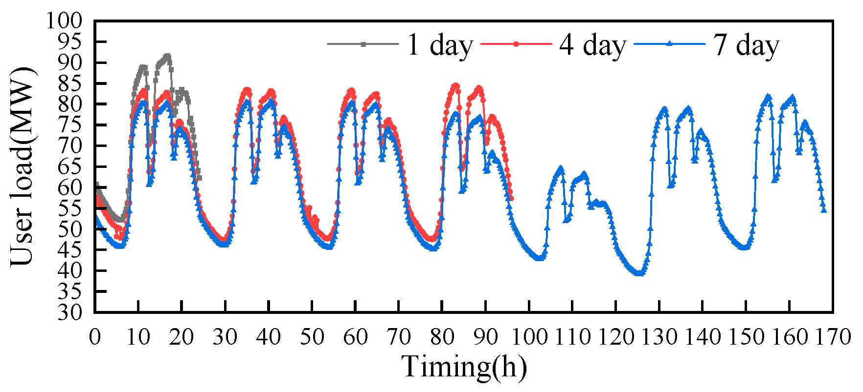
Figure 16.
Typical time power curve.
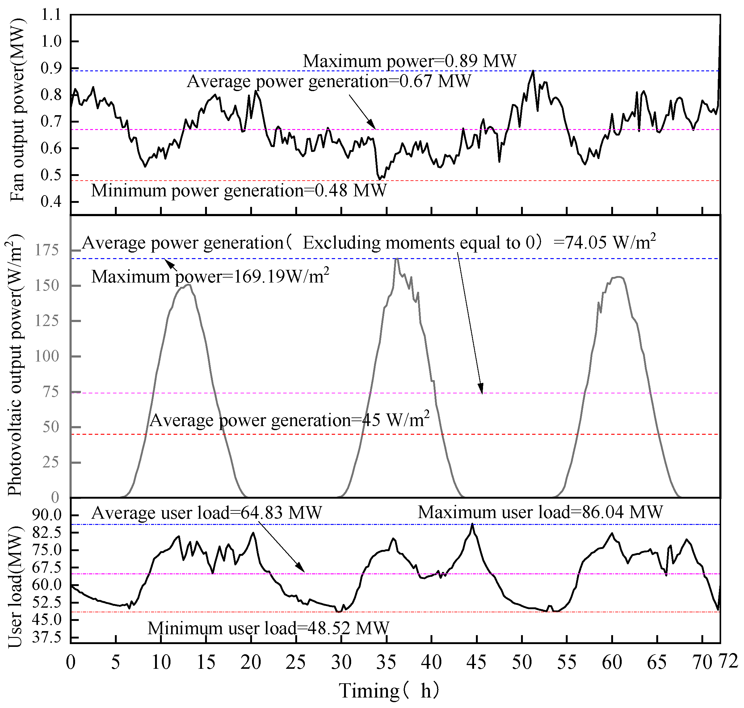

Table 1.
AW82/1500 wind turbine.
| Parametes | Rating (MW) |
Cut-in wind speed (m/s) |
Rated wind speed (m/s) |
Cut out air speed (m/s) | Blade length (m) |
| Value | 1.5 | 3 | 11 | 25 | 34 |
Table 2.
CY-TJ 250 photovoltaic panel.
| Parameters | Rating (W) |
Conversion efficiency(%) | Theoretical temperature(K) | Best angle (°) |
| Value | 250 | 25 | 296 | 30 |
Table 3.
Results of selection indicators for different typical time lengths.
| Name | 1 | 2 | 3 | 4 | 5 | 6 | 7 | |
| Wind energy | ΔC1 | 0.0112 | 0.0094 | 0.0087 | 0.0083 | 0.0089 | 0.0086 | 0.0090 |
| ΔC2 | 0.9643 | 0.9766 | 0.9853 | 0.9925 | 0.9923 | 0.9923 | 0.9919 | |
| ΔC3 | 0.0471 | 0.032 | 0.0217 | 0.0136 | 0.0138 | 0.0149 | 0.0139 | |
| Photovoltaic | ΔC1 | 0.0141 | 0.0125 | 0.0109 | 0.0126 | 0.0137 | 0.0153 | 0.0168 |
| ΔC2 | 0.9835 | 0.9885 | 0.9839 | 0.9803 | 0.9699 | 0.9626 | 0.9516 | |
| ΔC3 | 0.0394 | 0.0241 | 0.0267 | 0.0343 | 0.0413 | 0.0457 | 0.0460 | |
| Burden | ΔC1 | 0.0182 | 0.0116 | 0.0076 | 0.0151 | 0.0188 | 0.0209 | 0.0264 |
| ΔC2 | 0.9634 | 0.9747 | 0.9822 | 0.9746 | 0.9725 | 0.9535 | 0.9486 | |
| ΔC3 | 0.3423 | 0.2513 | 0.0125 | 0.0241 | 0.0417 | 0.0523 | 0.0619 | |
Table 4.
Results of selection indicators for different typical time lengths.
| Norm | Wind power | Photovoltaic | User load | ||||||
| ΔC1 | ΔC2 | ΔC3 | ΔC1 | ΔC2 | ΔC3 | ΔC1 | ΔC2 | ΔC3 | |
| Value | 0.1333 | 0.1334 | 0.1333 | 0.0333 | 0.0334 | 0.0333 | 0.1667 | 0.1667 | 0.1666 |
Table 5.
Results of selection indicators for different typical time lengths.
| Norm | Wind power | Photovoltaic | User load | ||||||
| ΔC1 | ΔC2 | ΔC3 | ΔC1 | ΔC2 | ΔC3 | ΔC1 | ΔC2 | ΔC3 | |
| Value | 0.1465 | 0.1759 | 0.0976 | 0.0428 | 0.0514 | 0.0105 | 0.1769 | 0.1801 | 0.1183 |
Table 6.
Results of selection indicators for different typical time lengths.
| Norm | Wind power | Photovoltaic | User load | ||||||
| ΔC1 | ΔC2 | ΔC3 | ΔC1 | ΔC2 | ΔC3 | ΔC1 | ΔC2 | ΔC3 | |
| Value | 0.1414 | 0.1595 | 0.1114 | 0.0391 | 0.0445 | 0.0193 | 0.173 | 0.1749 | 0.1369 |
Disclaimer/Publisher’s Note: The statements, opinions and data contained in all publications are solely those of the individual author(s) and contributor(s) and not of MDPI and/or the editor(s). MDPI and/or the editor(s) disclaim responsibility for any injury to people or property resulting from any ideas, methods, instructions or products referred to in the content. |
© 2025 by the authors. Licensee MDPI, Basel, Switzerland. This article is an open access article distributed under the terms and conditions of the Creative Commons Attribution (CC BY) license (https://creativecommons.org/licenses/by/4.0/).
Copyright: This open access article is published under a Creative Commons CC BY 4.0 license, which permit the free download, distribution, and reuse, provided that the author and preprint are cited in any reuse.


