Submitted:
30 June 2025
Posted:
01 July 2025
You are already at the latest version
Abstract
The electric Level 4 connected automated vehicles (CAVs) are now allowed in several cities around the world to demonstrate their automation capability in shared mobility robotaxi and microtransit services in geofenced areas. Private and public sector stake-holders need predictions of their adoption without regulatory constraints for personal mobility and use in shared mobility services. In anticipation of the future presence of CAVs in transportation vehicle fleets, governments are planning necessary regulatory and infrastructure changes. Accompanied with the need for forecasts is the acknowledgement that CAV adoption decisions must be made under uncertain states of technology and infrastructure readiness. This paper presents a Bayesian predictive modelling framework for electric Level 4 CAV adoption in the 2030-2035 application context. The inputs to the Bayesian model are obtained from effectiveness estimates of CAV applications that are processed with the Montecarlo method to accounts for uncertainties in these estimates. Scenarios of CAV adoption in the 2030-2035 period are analyzed using the Bayesian model, including the quantification of the value of new information obtainable from demonstration studies intended to reduce uncertainties in technology and infrastructure readiness. The results show that in the 2030-2035 application context, the CAVs are likely to be adopted, provided that the trajectory of progress in technology and infrastructure readiness continues, and potential adopters are offered opportunities to learn about Level 4 CAV technological capabilities in real life service environment. The findings of this research can be used by private and public sector interest groups.
Keywords:
electric connected automated vehicle
; Level 4 automated vehicle
; CAV adoption
; Bayesian model
; ride hailing
; robotaxi
; microtransit
1. Introduction
Automation in driving continues to attract research, development, and demonstration activities around the world. Substantial investments have already been made by the private as well as the public sector and more are needed to further advance the technology and related infrastructure readiness for adopting electric Level 4 connected and automated vehicles (CAV) without regulatory constraints. The Society of Automotive Engineers (SAE) International has defined five levels of automation noted below [1].
Level 1: Driver Assistance
Level 2: Partial Driving Automation
Level 3: Conditional Driving Automation
Level 4: High Driving Automation
Level 5: Full Driving Automation
Some new model vehicles with automation Levels 1 to 2 are already in the market. At presence, the availability of Level 3 automated vehicles in the market is very scarce and regulatory approvals are needed for their use. Level 4 CAVs are now allowed in several cities around the world to demonstrate their capability to operate in shared mobility ride hailing robotaxi service in geofenced areas. Also, demonstrations of slow speed Level 4 shuttles in microtransit service are underway with similar constraints. In these services, a safety technician is either onboard or monitors operations remotely [2,3]. Public road and highway authorities have initiated the process of accommodating automated vehicles, but so far there is a lack of uniformity in infrastructure changes and regulations.
The adoption of Level 4 CAV is of research interest in this paper. It features “high driving automation; the sustained and operational design domain (ODD)-specific performance by an advanced driving system (ADS) of the entire dynamic driving task (DDT) and DDT fallback without any expectation that a user will need to intervene” [1].
Looking ahead, Level 4 CAVs, have the potential to become mass market transportation solutions for personal mobility and robotaxis for shared mobility [4,5]. Likewise, the growing use of larger Level 4 shared mobility vehicles in microtransit demonstration service is an indicator of their future potential [6,7,8,9].
At an advanced level of development and when fully supported by necessary infrastructure, electric Level 4 CAVs have the potential to offer benefits to private owners, shared mobility commercial service investors (i.e., robotaxi fleet owners), and public agencies as well as private sector investors interested in their use in microtransit service. For this reason, the potential purchasers and deployers of Level 4 CAVs continue to be keen on learning about timing estimates for their implementation [9]. Although insights on this complex subject are provided by published literature, there is a need for a new predictive modelling framework that can treat uncertainties in technology and infrastructure readiness in forecasting electric Level 4 CAV adoption [9].
This paper presents research on a predictive model for electric Level 4 CAV adoption for the 2030-2035 market context. Specifically, the research is intended to meet the following objectives:
- (1)
- Predicting the effectiveness of electric Level 4 CAVs under uncertain states of technology and infrastructure readiness, in three applications, namely (a) private mobility, (b) robotaxi shared mobility, and (c) shared mobility microtransit service.
- (2)
- Treating uncertainties in effectiveness estimates using the Montecarlo method and producing two probability-weighted expected effectiveness estimates for each CAV application, one corresponding to relatively low level of technology and infrastructure readiness, and another corresponding to a higher level of readiness. These are needed as inputs to the Bayesian predictive model.
- (3)
- Formulation and implementation of the Bayesian model for predicting the probability of CAV adoption in 2030-2035 application scenarios of technology and infrastructure readiness states, including the quantification of the value of new information obtainable from demonstration studies intended to reduce uncertainties in the readiness states.
- (4)
- Obtaining insights from the predictive model results on conditions under which CAVs are likely to be adopted in the 2030-2035 period.
Although a Level 4 CAV is of interest in the industry as a freight vehicle, this application is beyond the scope of research reported in this paper.
Following this introduction, the methodological framework and its components are described. The functions of technology in their respective applications are explained. Next, the multi-criteria effectiveness method is applied to Level 4 CAV services and the Montecarlo method is used to account for uncertainties in effectiveness estimates. These results become inputs to the Bayesian predictive model. The theoretical foundation of the Bayesian model is explained, and applications are illustrated. The discussion section covers methods and results. Finally, conclusions are presented.
2. Methodological Framework
Attempts have been made in the past to study factors for defining timing estimates for CAV implementation in various service contexts. These studies were reported by public agencies or societies [9,10], independent researchers [11,12,13], consultants [14,15,16,17,18], and financial and related institutions [19,20,21,22,23,24,25]. A review of past studies suggests observations of interest to this research:
- Several interest groups are keen on learning about CAV adoption forecasts. These include: vehicle manufacturers and marketers, public sector infrastructure owners and operators, private sector transportation companies, financial institutions and investors, consulting firms, researchers, and consumer groups.
- Factors that could be used to forecast decisions on CAV adoption for various applications include technological capabilities, infrastructure for supporting CAV use, government regulations, differences between CAV and non-CAV travel characteristics, trends in general consumer acceptance of automation in driving, technology costs, and investor sentiments.
- With no substantive CAV market in place today, a methodological framework for forecasting must rely entirely on informed subjective estimates of CAV application effectiveness.
- Treating uncertainty in all inputs to a predictive model is necessary. Like-wise, all parts of the Bayesian model support decision-making under uncertainty.
Given current interest in forecasting many facets of CAV applications, a modelling framework shown in Figure 1 is defined and used in this research. Here, a brief overview of the framework and its components is noted, and theoretical and methodological details are provided in the following sections of the paper.
The first two boxes in Figure 1, labelled as “inputs”, define necessary information on technology and service context, characterize uncertain states of technology and infrastructure readiness, define effectiveness criteria, and use of the Montecarlo simulation method to obtain probability-weighted expected effectiveness estimates that are required by the Bayesian predictive model. The third box shows parts of the Bayesian model. Taken together, these provide answers to questions on conditions under which CAV adoption will become likely and the role of new information obtainable from demonstrations in reducing uncertainty in CAV adoption for three applications, namely private mobility, shared mobility robotaxi, and shared mobility microtransit service.
The methodological framework development was guided by the following requirements:
- Working with effectiveness criteria that can be quantified largely in non-monetary terms (e.g., user satisfaction, technology malfunction).
- Due to uncertainties in technology and infrastructure readiness and user acceptance of CAVs (i.e., for personal mobility, as a shared mobility vehicle), the method should be able to work with a range of criteria achievement levels.
- Use of a widely used method to account for uncertainties in criteria achievement levels and to produce probability-weighted expected effectiveness outputs required as inputs to the Bayesian predictive model.
-
Need for a predictive model with the following necessary capabilities:
- (a)
- Application of probabilities to uncertain states of technology and infrastructure readiness.
- (b)
- Enabling a role for new information on uncertain variables, obtainable from demonstrations.
- (c)
- Updating probabilities of uncertain states of technology and infrastructure readiness using the new information.
- (d)
- Producing answers to the value of new information in reducing uncertainties and enhancing the basis for CAV deployment decision for services defined above.
3. Overview of Level 4 CAV Technology and Infrastructure
The Level 4 CAV’s high driving automation capability is noted in the introductory section of the paper [1]. Communication technologies and equipped traffic control methods will be needed for supporting connected vehicle applications. Although an automated vehicle can function using traffic signals that are not digitized, but digital infrastructure can improve efficiency and safety. An automated vehicle can operate using existing infrastructure with the use of cameras and sensors to interpret control setting, digitally enhanced systems such as those used for vehicle-to-everything (V2X) can be used for real-time information exchange.
Transportation agencies are advancing V2X communications, which enable direct communications between devices. The dedicated short-range communications (DSRC), cellular (4G/5G), and potentially satellite networks have relevant roles to paly for CAV operation [26,27,28,29].
For technology and supporting infrastructure to be considered at an advanced stage of development, significant CAV technology advances as well as extensive supporting technology implementation in the road traffic network will be needed. Some forecasters go beyond these requirements by suggesting the integration of mobile devices carried by pedestrian and bicyclists into the V2X ecosystem [26].
Public and private sector investments in automation in driving research, development and demonstration (RD&D) have not yet advanced the state of technology to the extent that deployment of Level 4 CAV can be planned with certainty of only positive effects and avoiding negative impacts.
For the foreseeable future, it is necessary for technology regulators and investment decision-makers to work with uncertain states of technology and infrastructure readiness. In the following sections of the paper, in the 2030-2035 service context, forecasts of positive as well as negative attributes of the Level 4 CAV technology are described for two uncertain states: relatively low readiness of technology and infrastructure & relatively high readiness of technology and infrastructure.
4. 2030-2035 Service Context
4.1. Private Mobility Vehicle
This vehicle will be owned and maintained by the owner. The batteries can be charged at several locations (i.e., at the residence of the owner, at work location, at a commercial fast charging station, etc.) [30]. These vehicles will be used for all travel purposes in the city, on intercity routes and on rural roads. Availability of communication service will enable the use of automation as well as connected features of the technology. The presence of a human driver in the driver’s seat strengthens the safety attribute of the Level 4 CAV private mobility vehicle.
4.2. Robotaxi
Following regulatory approvals, fleets of electric Level 4 CAVs can be deployed in ride-hailing robotaxi service without geofence limitation. Passengers can request a CAV using an App. The robotaxi system, also known as shared automated vehicle (SAV) system, consists of vehicles, stations for parking, battery charging, and among other functions, devices to monitor and control CAV fleet. As a commercial business, these systems are expected to become economically feasibility [31].
Even in their current state of development, shared automated vehicle applications are planned around the world [32]. Robotaxis operate in well-defined geofenced areas in several cities around the world without a safety driver in the vehicle (but in a control center). The technology has advanced to the extent that it makes it unnecessary to have a human safety driver in the vehicle. Instead, a remote-control center is used for surveillance and emergency correction of the driving functions. These specially designed centers are connected with robotaxis, using a combination of wireless communication technologies, for real-time support and guidance in situations that exceed their automation capabilities.
The communication technologies used include cellular networks (4G/5G), V2X communication, and potentially satellite communication for locations with limited cellular coverage. Human operators in the control center monitor service operations and resolve potential issues. The communication system enables them to provide navigation assistance, re-route the vehicle, or manage unexpected conditions. The knowledge that the remote human operator can assist the CAV contributes to user trust in the system.
4.3. Microtransit Service
Microtransit, as a shared mobility system, is experiencing rapid growth. It is defined as “Privately or publicly operated, technology-enabled transit services that typically use multi passenger/pooled shuttles or vans to provide on-demand or fixed schedule services with either dynamic or fixed routing”[33,34]. Many public transit service gaps are addressed by microtransit, including the first/last mile connectivity that enables travelers to complete the origin-to-destination trip [35].
In 2030-2035, the right-sized electric Level 4 CAV will be able to provide a cost-effective on-demand microtransit service without a safety driver in the vehicle. Avoiding the driver’s cost greatly enhances the cost-effectiveness of the service. Research shows that the driver cost for an accessible battery electric non-automated minibus with 19 seats accounts for 43% of vehicle cost [35]. Although the Level 4 CAV-based microtransit system is monitored by a control center, its cost does not adversely affect the feasibility of the service [33]. For information on the communication technologies that enable the CAV fleet to connect with the control center and the role of the human operator in the control center, please see the above robotaxi section.
5. Level 4 CAV Technology and Infrastructure Attributes
5.1. Positive Attributes (2030-2035 Service Context)
Following necessary public sector regulatory approvals, Level 4 CAV deployments can be planned. As noted earlier, in this research, the following are of interest: personal mobility, robotaxi service, and CAV-based microtransit service. Details of these applications are presented in Section 4 of the paper. Here the attributes of technology and associated infrastructure are described. These, in essence, serve as effectiveness criteria of CAV deployments and are key variables that influence trust in and acceptance of CAVs.
The following four positive effects of electric CAV applications are commonly described in the literature:
- Human factors-related collisions avoided (safety benefit).
- User satisfaction (as owner of the personal passenger vehicle, user of the robotaxi service, user of the CAV-based microtransit service).
- Socio-economic benefits (other than safety benefits).
- Environmental benefits.
The main rationale for favorable public policies regarding automation in driving is to reduce traffic accidents caused by human errors [27,28,38]. The CAVs can potentially avoid collisions due to a combination of advanced sensors, algorithms, and communication with vehicles and infrastructure [39]. According to a UK source, human errors account for 88% of all road collisions, making CAVs a potentially transformative safety technology [40].
User satisfaction with Level 4 CAVs is a multifaceted attribute. Survey of consumers show that they like the availability of automation features (14). But their acceptance is unlikely without trying its technological capabilities using a demonstration vehicle. Potential owners can benefit from greater levels of safety (covered above). Convenience features add to the user satisfaction, including the ease of operation for parking, merging, and other maneuvers. Numerous publications have covered the subjects of user acceptance and trust models [41,42,43,44]. These studies found the main variables to be the same as the ones defined here as positive attributes and avoiding the negative attributes described in the following section.
Traveler acceptance of the robotaxi service remotely monitored by a control centre is subject to uncertainty. Likewise, accepting a microtransit shuttle vehicle monitored by a remote-control centre may be viewed differently than travelling in a slow-speed demonstration shuttle with a technician in the vehicle. Therefore, user/traveler acceptance of Level 4 CAV cannot be assumed with certainty.
More than sixty factors of expectation, experience, acceptance of automation in public transportation were identified by review articles [42,43,44]. Frequently cited desirable service factors include seat availability, comfort, being on-time, schedules, fares, road safety, onboard safety and security, and cyber security. Traveller personal factors also known to influence their acceptance (e.g., socio-demographics, travel habits, personality).
Interviews of demonstration shuttle vehicle users s carried out before and after travel, in general, did not show major concerns. Models developed suggest acceptance of automated shuttles in the future, subject to absence of technical issues and a clearer explanation of legal responsibilities in case of an accident [42,43,44].
The CAVs offer recognized socio-economic benefits, including increased safety (covered above). Specifically, some socio-economic benefits noted by survey respondents are improved mobility for those who are unable to drive due to age, disability, or other reasons, enhanced accessibility for underserved populations, and affordable shared mobility. [28,45].
Electric CAVs offer environmental benefits when used for personal mobility and in shared mobility services [32]. To maximize environmental benefits, large-scale market penetration of electric CAVs as well as availability of battery charging infrastructure are necessary. Towards this end, increased public and private sector efforts are needed to secure public and consumer trust [46].
5.2. Negative Attributes (2030-2035 Service Context)
The following four negative effects of electric Level 4 CAV applications are commonly described in the literature:
- Technology unreliability.
- Effect on other road users.
- Hacking and data security.
- Cost differential (i.e., extra cost of automation).
Although in the 2030-2035 service context, the Level 4 CAV technology and supporting infrastructure are expected to be more advanced than now, these may still be in need for further development (i.e., these may not be considered as “mature”). Surveys of potential adopters and technology experts suggest that at the present state of development, technology unreliability is a concern. Further advances will be necessary before the Level 4 CAV will be ready to avoid collisions in edge cases and therefore serve the market without regulatory conditions. In this context, potential users consider occupants’ safety and legal liability in case of an accident as issues that should be addressed [41,47].
The need to improve the reliability of sensors in the Levels 4 CAV has been noted in the literature. Therefore, continued R&D efforts are needed so that these become fully ready for widespread deployments in all environments. At their present state of development, these can operate safely in specific and well-defined conditions in geofenced areas without a safety driver onboard. But for future increased scope of operations, technology advances and supporting infrastructure readiness are necessary [32,48].
Crash data for CAV Levels 3-5 show that as automated vehicle usage increases, crashes increase as well, and technology malfunction may be one of the causes [49]. Survey results suggest that public concern about technology unreliability increases with the automation level [46]. Studies of the American Automobile Association (AAA) Foundation for Traffic Safety show that the public as well as technology experts recognize the importance of the safety attribute of CAVs and they are concerned about technology malfunction [50,51]. Other surveys found similar safety concerns [32].
The effect of CAV operation on other users of the road needs designer attention. Given that multiple accidents have occurred between automated vehicles and pedestrians, this concern is not without evidence [32]. Recognizing the importance of minimizing adverse effect of CAV operation on vulnerable road users, R&D efforts continue to address challenges in their interaction. Specifically, efforts are reported to improve technology (e.g., algorithms, training, dataset) for enhanced accuracy in all types of interactions [52].
Cybersecurity and data privacy will continue to be challenges in future years due to the reason that the Level 4 CAV features a large attack surface which makes it vulnerable to cyberattacks. Although the connectivity attribute of the CAV system offers safety and convenience benefits, without safeguards, it becomes a vulnerability that can be exploited by hackers [53,54,55].
The cost difference between a CAV and a vehicle without connected and automated technologies in 2030-2035 application period is another attribute of interest in this research. The consumer survey results suggest concerns with purchase and on-going maintenance costs of the Level 4 CAV [50]. A forecasting study suggests that automation will add 20% to the cost of a vehicle [56]. Although the cost differential between electric CAVs and conventional technology vehicles will improve in favor of CAVs, it is not likely to be zero. The price difference is expected to considerably decrease over time due to the following reasons: technology advancements, increased competition, and mass production. In the case of shared mobility services, all costs (i.e., purchase, operations, maintenance and management costs) are expected to drop due to higher vehicle utilization, increased ridership, wider operating areas, and service optimization [32].
6. Uncertain States and Decision-Making Under Uncertainty
A decision to adopt Level 4 CAV will be made by a decision-maker or decision-makers under uncertainty. It is assumed that the decision to adopt the CAV for individual mobility will be made by the owner. The decision to adopt the CAV for robotaxi service will be a corporate decision. Likewise, the decision to adopt the CAV shuttle for microtransit service will be made by the fleet procurement manager on behalf of the organization. The variables for modelling the decision-making problem are shown in Table 1. It is understood that government regulations will allow the sale and use of CAVs for the licensed service. Although regulations may permit demonstration services in limited conditions as is the case now, these permits do not imply commitment to allowing full-scale deployments without further technology and supporting infrastructure improvements.
Many technology and infrastructure attributes can be assessed to infer the state of readiness for Level 4 CAV adoption. Key attributes are safety and reliability of technology (including occupant safety and security, safety of other road users), favorable record of cybersecurity and safeguarding data, successful human-machine interfaces as required for Level 4 CAV operation (including verification that in the case of shared mobility services, the remote control staff can indeed resolve issues), consumer acceptance of cost of automation in driving, resolution of legal responsibility in case of accident, and favorable record of operating permits granted by regulatory authorities without geofencing and other constraints.
The state of technology and infrastructure readiness in the 20230-2035 CAV implementation period cannot be predicted with certainty. There are many key actors who play RD&D and permitting roles according to their objective function. These include vehicle producers and providers, infrastructure owners and operators, private transportation companies, financial institutions and investors, consulting and strategy firms, researchers, public officials and politicians, and consumers [9].
Technological forecasting studies such as the one reported in this paper must work with relevant influencing factors for which objective data may not be available. Therefore, reliance is placed on subjective estimates. In this research, despite efforts in sourcing objective data/estimates, it is necessary to rely on informed subjective information regarding the following variables: trajectory of technological capabilities, government regulations, shifting travel behavior, perception of benefits obtainable from CAVs as compared with non-automated vehicles, general consumer trends, technology costs, and investor sentiment [9].
The impacts/consequences/effects of a combination of an adoption decision A and a state of technology and infrastructure readiness state S (i.e., A&S) are quantified in relative value (utility) metrics [57]. As explained in the following section of the paper, there are well established theoretical and practical reasons for using utility metrics in this study of CAV adoption for applications noted in Table 1.
7. Quantifying the Effectiveness of CAV Application in Meeting Owner/User Criteria
7.1. Utility (Relative Value) Theory
In Section 5.1 and Section 5.2, eight attributes of Level 4 CAV application are discussed. Since these characterize the effects of adopting the CAV (e.g., collisions avoided, user satisfaction, technology malfunction incidents), these serve as effectiveness criteria. Although some criteria can be quantified in their respective units (e.g., accidents avoided, number of technology malefaction incidents), other will require relative value units (e.g., user satisfaction, many and diverse nature of socio-economic benefits). Also, market values do not exist for most effects. For these reasons, these effects cannot be quantified in monetary units or in units of any other criterion. Well-recognized methods are available for researching this type of socio-technical problem. Following the study of manuals and application examples, the multi-criteria analysis method in association with utility metric was adopted to quantify the effectiveness of Level 4 CAV applications for personal mobility, shared robotaxi service and shared mobility microtransit service [38,57].
The effectiveness of a CAV application can be expressed as:
where
e is effectiveness of Level 4 CAV application.
Cri achievement level, by the CAV, of a criterion i, i = 1,2, …, q.
e(Cri) is the utility of achieving Cri (e.g., collisions avoided).
i(Cri) is the probability that Cri will be achieved by the CAV application (e.g., robotaxi).
The methodology permits the consideration of differential effects (e.g., safety of various vulnerable users of the road). In such a case, the hth level of criterion g, Crgh, which can occur due to CAV operation, can be expressed as:
Crgh = the hth level of criterion g (e.g. safety), weighted for all affected groups
where
= k1Crg1 + k2Crg2 + k3Crg3 + ….. + ksCrvg
Crgv = the level of achievement of criterion g for group v (e.g., safety for group v – pedestrians, etc.)
kv= a weight, reflecting the importance of the impact group v with respect to criterion Crg, and can be determined from the societal (community’s) preference expressed as ranks such that v = 1.0.
The scale for measuring positive criterion achievement is 0 to 100 and for negative criterion, 0 to -100 is used. The criterion achievement values (called effectiveness values) are based on potential technology improvements (i.e., past or current observations cannot be used). It is a very challenging but essential task to assign values for various levels of criteria achievement (e.g., utils for avoiding collisions). Commonly available statistics, user surveys or opinions of experts are used as guides for this purpose.
The quantification of criterion achievement levels follows the axioms of the utility theory [57]. As noted above, the utility value is a relative measure of the degree to which each criterion is achieved by a CAV application. Since positive and negative scales are used in this research, the utility theory permits the addition of values measured on positive and negative value scales.
Due to lack of objective information on Level 4 CAV technology and supporting infrastructure in the 2030-2035 application context, single values of criterion achievement cannot be assigned with certainty. Therefore, the following methodological steps are applied to account for uncertainty.
The effectiveness values are estimated as ranges, the higher the degree of uncertainty, the wider are the estimates.
- The Montecarlo method, described in the following section, is applied to calculate the probability-weighted expected value of criterion achievement.
- Next, the expected value of criterion achievement level obtained from Montecarlo simulation can be transformed, if warranted.
The process of transforming the expected criterion achievement level obtained from the Montecarlo method into utility units (utils) is illustrated in Figure 2. Three types of utility functions are shown that can be used for scale transformation purposes: a non-linear function that exhibits diminishing marginal value, a linear transformation function with an intercept, and another linear function without an intercept.
For the non-linear case:
where
e(Cri) = H[Cri (Cri measured on the original value scale)]z for z<1 and i= 1,2, …,q
e(Cri) = the utility measure, in transformed units, for criterion Cri.
H and z are constants.
For the case of linear transformation with an intercept:
where
e(Cri) = miCri + bi for i = 1,2, …, q
mi = slope of the transformation curve for Cri
bi = vertical axis intercept (if applicable, a threshold step can be applied).
The origin of the scale can be set in any desirable way. For the example evaluations presented in this paper, 0 ≤ e(Cri) ≤100.0.
Although in explaining the theory, and as illustrated in Figure 2, three utility functions are noted, due to lack of experience with electric Level 4 CAV applications, only linear transformation without intercept is used. However, for future use of the methodology, it is useful to note that the utility functions can be derived from stated preference or revealed preference surveys of consumers/interest groups. If sufficient data become available to estimate the non-linear utility function, it may exhibit the property of diminishing marginal utility.
The expected effectiveness of an electric Level 4 CAV application j in 2030-2035 is obtained as:
where
ej = ∑ i=1 to q [wi.(eCri)]
ej = expected effectiveness of CAV application j, weighted for all impact/interest groups
wi = weight assigned to criterion i
The expected effectiveness method is applied to three electric Level 4 CAV applications: personal mobility vehicle, shared mobility robotaxi service, and share mobility microtransit service. Details of input information, intermediate computations, and results are reported in Sections 7.3 to 7.5.
7.2. Montecarlo Method to Treat Uncertainties
The Montecarlo method uses random numbers to sample probability distribution functions for computing expected value and standard deviation. In this research, instead of using the middle values of the range of uncertain effectiveness estimates, these are analyzed using the scientific Montecarlo simulation method. The use of this theoretically sound and well recognized scientific method was suggested by the US DOT for the IntelliDrive benefit-cost analysis [58]. An introduction to simulation and Monte Carlo methods can be read in Rubinstein and Kroese [59] and Evans et al. describe characteristics of probability distribution functions and their suitability for various applications [60]. The Montecarlo method is suitable for use in this research due to its ability to work with a range of values of uncertain variables (i.e., minimum and maximum values), application of probabilities sampled from specified distributions, and if applicable, treating peaking of values.
A rectangular (also called uniform) probability distribution function and a triangular probability distribution function are well suited for the analysis of stochastic effectiveness variables and are therefore used in this research (Figure 3 and Figure 4). The Montecarlo method draws samples from their cumulative probability distribution functions using random numbers.
The continuous uniform probability distribution function is characterized by two values: the minimum value α and the maximum value β. This distribution is used to represent a higher uncertainty regarding the phenomenon under study by treating all values of the random variable as equally probable. In scientific terms, this probability distribution is the maximum entropy probability function for a stochastic variable denoted as X [59].
The statistical characteristics of the continuous uniform probability distribution function are noted below.
Probability density function: P(X) = 1/(β-α) for X ϵ |α,β| and 0 otherwise
Mean: ½(α+β)
Median: ½(α+β)
Mode: any value in (α,β)
The continuous triangular probability distribution function is defined by the minimum value α, the maximum value β, and the peak (i.e. the mode or most likely) value λ. This probability distribution function has been widely applied in real-life problem-solving conditions under uncertainty due to its ability to treat the minimum and maximum values, and the most frequent outcome (i.e., the mode). These values can be assigned without knowing the difficult to obtain mean and the standard deviation of the values of the variable of interest. By assigning definite lower and upper limits, the analyst can bypass the assumed extreme values. Further, this function enables the treatment of skewed probability distributions [59].
The main statistics of the triangular probability density function are noted below.
for α ≤ X ≤λ and
P(X)=2(X-α)/[(β-α)(λ-α)]
2(β-X)/[(β-α)(β-λ)] for λ≤X≤β
Also, P(X) = 0 for X<α and X>β
Where λϵ|α,β|is the mode
The mean is 1/3[(α+β+λ)]
7.3. Computation of Criteria-Weighted Effectiveness
7.3.1. Effectiveness Criteria Weights
In Section 7.1., the theorical foundation of the effectiveness method is described. Here, components of Equation 5 are developed. The criteria weights suggested for use in this research are shown in Table 2. Safety and security criteria are assigned higher importance than other criteria. These weights reflect surveys of potential users of electric Level 4 CAVs. Examples of notable surveys were carried out by the Foundation for Traffic Safety of the American Automobile Association (AAA) [51] and the McKinsey & Company [32,61]. The raw weights on a 0-10 scale are normalized for use in Equation 5.
7.3.2. Private Vehicle Effectiveness
In accordance with the methodology, the criteria effectiveness values are assigned on a 0 to 100 scale for Cr1 to Cr4 and on a 0 to -100 for criteria Cr 5 to Cr 8 (Table 3). The values reflect conditions under the low state of technology and infrastructure readiness scenario S1. The basis for subjectively assigned values is a pessimistic view of technological projections for the 2030-2035 period. Literature cited in Section 3, Section 4, Section 5 and Section 6 provided sufficient information for the relative effectiveness values. As previously noted, the effectiveness values (+ve & −ve) are estimated as a range of values due to estimation under uncertainty.
In columns 3 and 4 of Table 3, the expected effectiveness values and St. deviations results of the Montecarlo method are shown. The results obtained with the use of uniform probability distribution function in general reflect higher uncertainty as compared to the triangular probability distribution function. In the last column of Table 3, the weighted effectiveness values are based on uniform probability distribution results and normalized weights shown in Table 2. In accordance with the axioms of the utility theory, the utility values can be added. The -9.1 utils is the answer obtained for Equation 5. The negative sign indicates that if the uncertain state S1 (i.e., low state of technology and infrastructure readiness) becomes true, the Level 4 CAV use as a private vehicle is not favorable.
Table 4 presents the inputs and results for Level 4 CAV for the scenario of higher state of technology and infrastructure readiness (i.e., S2). That is, if S2 becomes true, the likely effectiveness values and the final weighted effectiveness results of Equation 5 will be as shown in Table 5. As expected, in comparison with the lower state of technology and infrastructure readiness, under higher state of technology and infrastructure readiness, the CAV use as a private vehicle is favorable.
7.3.3. Ride-Hailing Robotaxi Effectiveness
Table 5 and Table 6 provide inputs and results for the Level 4 CAV used for ride-hailing robotaxi service. Under both S1 and S2 states, the ride hailing robotaxi is slightly more effective than the private mobility vehicle. Although the CAV used for ride-hailing robotaxi service is technologically like the CAV used as a private vehicle, there are minor differences in effectiveness values. The private vehicle owner is likely to experience a somewhat higher satisfaction than a robotaxi user. The robotaxis are monitored by professional staff and in comparison, the human driver in the private mobility vehicle may not always be fully alert in case a corrective action is needed that the automated system may not be able to handle. Another difference is regarding the cost of automation. Due to fleet discounts the robotaxis are likely to be better off than a private vehicle.
7.3.4. Microtransit Vehicle Effectiveness
The effectiveness values for the Level 4 CAV used for microtransit service under S1 and S2 states are presented in Table 7 and Table 8. Under S1, user satisfaction is higher for robotaxi than for microtransit, but microtransit has higher overall effectiveness value than for robotaxi. Under S2, user satisfaction is higher for robotaxi than for microtransit, but microtransit has higher scores than robotaxi for hacking and automation cost. On the balance, the weighed effectiveness score is higher for the CAV in microtransit service than for the CAV used as a robotaxi. The differences arise due to closer monitoring of microtransit CAV operation and management than robotaxis, and microtransit CAVs receive a higher fleet discount and incur lower operation and management costs.
8. Bayesian Model: Theory
The technological forecaster needs methods that can identify high payoff paths under uncertainty. The Bayesian model is widely accepted due to its capability to work with uncertain states of nature and estimates of gains that are expected to result from action-state combinations. In this research, the uncertain states of technology and infrastructure readiness are S1 & S2 in the 2030-2035 application context and potential actions are adoption decisions on CAV applications. The weighted effectiveness results (i.e., effectiveness of CAV adoption under S1 & under S2) presented in Table 3, Table 4, Table 5, Table 6, Table 7 and Table 8 become inputs to this method.
Within the field of statistical methods for decision-making under uncertainty, the Bayesian analysis offers the required capability to model technological forecasting problems. It allows the forecaster to use prior probabilities for the occurrence of uncertain states of nature and offers the ability to update probabilities using new information obtainable from learning methods (i.e., demonstration studies). In the Bayesian method, as explained below, probabilities have important roles in risk analysis.
Considerable efforts have been underway by stakeholders from research institutes, industry, and government to provide the latest information to the public on CAV’s capabilities as well as their limitations. Technical forums provide information and examine the impact of information on consumer understanding of automation in driving. User surveys carried out before and after the use of a demonstration service are useful to gauge change in potential adopter views and confidence.
Given the importance that potential adopters attach to the “need to test it personally”, demonstration of technology is assumed for all analyses. At the time of the demonstration activity, questions on technology, infrastructure, and regulations can be answered. As explained later, the Bayesian model can quantify the change in perceived gain of CAV adoption due to availability of new information obtainable from learning about technology and infrastructure readiness during demonstrations and related question & answer sessions.
Selected example applications of the Bayesian decision theory to model forecasting problems can be read in references [62,63,64,65,66]. These papers show that logical answers were obtained that could not be obtained with other known methods. If a forecast is to be made or a highly desirable course of action is to be identified under uncertainty and it is possible to learn from new information to modify probabilities of the uncertain future conditions, the Bayesian theory is best suited to analyze the problem.
8.1. Prior Analysis
For modelling the CAV adoption decision under uncertainty, the decision maker is to be known. Table 1 provides this information, and it is repeated here for ease of reference. In the case of Level 4 CAV ownership, the decision maker is the individual consumer. For the robotaxi fleet, the decision maker is the corporation. In the case of microtransit vehicle fleet, the decision-maker is the public transit agency. On the other hand, in the case of a privately owned system, the investor is the decision maker.
To add to the previous descriptions, variables of the CAV adoption decision model are defined below:
- Alternatives: A1 adopt CAV; A2 do not adopt CAV.
- The condition under which adoption decision will be made is characterized by the following uncertain states of technology and infrastructure readiness: S1 low state of technology and infrastructure readiness; S2 higher state of readiness.
- The impact (consequence) of each A&S combination is quantified by the expected weighted effectiveness values presented Table 3, Table 4, Table 5, Table 6, Table 7 and Table 8. In Bayesian analyses, these are termed as Gain G of CAV adoption. Depending upon the specific A&S combination, the G can be negative or positive.
- The uncertain states are assigned probabilities of occurrence. These probabilities are called prior probabilities. The term prior is used because the decision maker has the option to ask for a demonstration study and the new information can be used for revising prior probabilities into posterior probabilities.
In the prior analysis, the prior probabilities are applied to gain G for the applicable A&S combination to calculate probability-weighted expected gain. For the adoption of a selected CAV (i.e., private automobile or robotaxi or microtransit vehicle),
where
EXP(Gi) = the expected gain for alternative ; = 1 or 2. For example, for the private car, A1 represents adoption decision and A2 is used for no adoption.
= the gain of alternative , under uncertain technology and infrastructure readiness state ; = 1, 2
Pj = probability of state of nature Sj (i.e., technology and infrastructure readiness state).
Figure 5 shows the prior analysis part of the Bayesian model.
8.2. Posterior Analysis
The demanding technological forecasting task requires knowledge extraction from available sources as well as the option to initiate new information acquisition activity for use in converting prior probabilities to posterior probabilities. In the decision theory terminology, these initiatives are called learning experiments. In this research the term learning activity (L) is used. At the time of initiating an L about uncertain states of technology and infrastructure readiness, the outcomes are unknown and therefore probabilities are applied to their occurrence. Given two unknown states S1 and S2, the results obtainable for L are r1 (that corresponds to S1) and r2 (that corresponds to S2). The option of not initiating a learning activity is L0 and therefore r0 is the outcome.
The reliability of resulting information about the occurrence of uncertain states (i.e., S1 and S2) is another variable that is needed for revising the probabilities. The revised probabilities are termed posterior probabilities, and their application is known as posterior analysis. In statistical terms, the conditional probability P(r|S,L) enables conversion of prior probabilities to posterior probabilities of technology and infrastructure readiness states.
Equation 13 defined in the prior analysis section enables the analyst to compute the expected gain Gij of an alternative Ai, using prior probabilities Pj of uncertain states Sj. The resulting expected gain G is the answer obtained from the prior analysis part of the Bayesian method. Since the prior probability-based analysis does not include a role for new information intended for revising probabilities, the posterior analysis is the next logical step.
Raiffa and Schlaifer [67] defined the theoretical basis of posterior analysis, pre-posterior analysis and the value of new information obtained from a learning activity L. Figure 6 shows the sequence of decision-making under uncertainty in the posterior analysis case. The G(L,r,A,S) represents gains for all L,r,A,S combinations.
The Bayesian analysis requires the following probability distribution functions.
- Using the prior analysis as a base, the prior probability P’(S) for each S is required before observing the outcome r of the new information acquisition activity L.
- A conditional measure P(r|S,L) is to be assigned, which represents the probability that the result r will be observed if the learning activity L is carried out, and S is the true state. That is, the analyst should define the reliability of the information outcome r of L in predicting the true state S.
- The marginal measure P(r|e) is computed as shown next:P(r|L) = ΣP’(S) P(r|S,L)
- The posterior probability P”(S|r,L) can now be calculated using the Bayes Theorem:P”(S|r,L)=[P(r|S,L)P’(S)]/(P(r|L)
This equation reflects the Bayesian philosophy that an L can be characterized by a conditional probability P(r|S,L) (a reliability indicator), used for computing posterior probabilities. The Bayes Theorem (Equation 15) defines the relationship between the prior and posterior probabilities.
The decision trees for comparing the prior and posterior analyses are shown in Figure 5 and Figure 6. In the posterior analysis, the decision variables are L and A, and random variables are r and S. It is solved by moving from right to left. The value of a sequence of actions is represented by the gain G (L,r,A,S). The prior branch is solved using Equation 13. The equations for solving the posterior branch and comparison of results of both branches are presented in the following section. To compare L with L0, decision trees shown in Figure 5 and Figure 6 are analyzed. A comparison of results of posterior and prior branches leads to the quantification of the value of the new information (i.e., the value of pre-posterior information).
8.3. Pre-Posterior Analysis
The pre-posterior analysis is intended to quantify increase in gain obtainable from the learning activity L. This materializes due to risk reduction in the choice of the Level 4 CAV adoption. The following are the pre-posterior analysis steps. The starting point is the prior probability P’(S). For the L, the conditional probabilities P(r|S,L) are defined. The marginal probabilities P(r|L) for L are computed using Equation 14. For the null learning option L0, the marginal probability is P(r0|L0) = 1.0). The posterior probability P”(S|r, L) is computed for each combination of S and r (Equation 15). For each combination of L,r,A,S, its gain is found: G (L,r,A,S).
The expected gain for each alternative A in the posterior branch is as follows:
G*(A,r,L) = ∑S P”(S|r,L) G(L,r,A,S)
However, for the prior branch, where no new information is acquired,
G*(A,r0,L0) = ∑s P’(S) G(L0,r0,A,S)
For each (L,r) combination, the optimal alternative is determined, and its associated gain is noted:
G*(r, L) = MaxA G*(A,r,L)
For the information acquisition activity L, the expected gain can be computed:
G*(L) = ∑ r P(r|L) G*(r, L)
8.4. Value of New Information
The Bayesian decision theory enables the quantification of how much G can be improved (by reducing uncertainty) with new information before obtaining it. It is a unique decision-aid that enables the identification of conditions under which to initiate the new information acquisition activity L.
The computational steps are noted next and illustrated in Figure 7.
(1) From the posterior branch, for L and each r, find MaxAG*(A,r,L). Call it Ar.
(2) For L0 in the prior branch, find MaxG*(A). Call it A’.
(3) For each r, find (Ar-A’)
This is Vt(L,r), the terminal value for the (L,r) combination.
The subscript t represents terminal values.
(4) The expected value of new information is computed as follows.
Vt*(L)=∑r[P(r|L)(Ar-A’)]=∑rP(r|L)Vt(L,r)
The superscript * represents expected (i.e., probability-weighted) value.
Examples of Vt*(L) application are presented in the following sections. For brevity, thes are shown as Vt*.
9. Application of the Bayesian Model
The methodological framework illustrated in Figure 1 shows the process for preparing inputs to the Bayesian model and the steps for model implementation. Details of the Bayesian model are presented in Section 8.1, Section 8.2, Section 8.3 and Section 8.4. Within the Bayesian model, prior probabilities, conditional probabilities, and the gain information are the inputs. The outputs are the value of new information, the preferred adoption option and the corresponding expected gain value.
In populating the gains information, the results of the weighted effectiveness computations for the A&S combinations presented in Table 3, Table 4, Table 5, Table 6, Table 7 and Table 8 are used. For example, for the Level 4 CAV used for private mobility, the following G(A1,S1) = -9.1 utils is used and the contrary decision is assigned zero gain (i.e., G(A2,S1) = 0 utils). Under S2, G(A1,S2)= 14.1 utils and G(A2,S2)= 0 utils.
An important consideration in assigning zero gain for A2 (i.e., do not adopt) decision is that no positive or negative effect will result from not adopting the CAV for personal mobility. This philosophical argument is also applied to robotaxi and microtransit cases.The counter argument that under low technology and infrastructure readiness state S1, a positive gain (i.e., G(A2,S1) = 9.2 utils)) will occur as the opportunity value if the Level 4 CAV is not adopted, is difficult to justify and therefore is not pursued.
The Bayesian model is used to analyze scenarios for CAV adoption in 2030-2035 period to define conditions under which the CAV adoption will be likely. Also, it is of interest to define conditions under which the value of new information is positive (i.e., (i.e., when Vt* is > 0). A positive Vt* plays a role in reducing uncertainties and improves expected gain for the adopted Level 4 CAV.
An illustration of the effect of new information (i.e., r2 with conditional probability of P(r2|S2,L) = 0.7) on changes from prior to posterior probabilities can be observed in Figure 8. For example, starting from a rather low prior probability of P’(S2) = 0.4, in association with the high reliability of favorable new information (i.e., r2), the posterior probability rises to 0.609. This observation is useful in reviewing the results of analyses presented below.
For each Level 4 CAV application under study, the Bayesian model was run using the gain values described earlier. Two types of scenarios were analyzed. First, the prior probabilities were changed while keeping the conditional probability P(r2|S2,L) constant at a high level of 0.7. As noted previously, the conditional probability reflects the reliability of the new information acquisition activity L. Eleven scenarios were run with different prior probabilities of S1 and S2. The P’(S2) was changed from 0.05 to 0.9. Table 9, Table 10 and Table 11 present results. In the second type of scenario, the effect of changes in conditional probability P(r2|S2,L) were studied while the prior probability was constant. The results are presented in a later section of the paper.
9.1. Private Auto
The results of eleven scenarios of Bayesian model prediction of CAV adoption for private mobility are presented in Table 9. The first column shows prior probabilities. For S2, these were varied from 0.05 to 0.90. The second and third columns show conditional probabilities. These were held constant to distill the effect of changes in prior and posterior probabilities. Columns 5 and 6 show gain values for A&S combinations (i.e., G(A,S)). Column 7 presents the value of new information Vt* and column 8 shows the preferred adoption option and the corresponding expected value E(A). In the final column, results are interpreted.
The value of new information Vt* is positive from P”(S2|r2,L) 0.5 to 0.778. During this range of probabilities for technology and infrastructure readiness S2 state, new information plays a role in reducing uncertainties and therefore improves the expected gain of adoption of A1. The CAV adoption (i.e., A1) becomes the choice starting from P”(S2|r2,L) = 0.607 and its expected gain continues to rise from here to the last scenario.
9.2. Robotaxi
The Bayesian model results for the Robotaxi CAV are presented in Table 10 using the Table 9 format. The results differ somewhat from those for the private mobility CAV. The Vt* becomes positive sooner, starting with posterior probability P”(S2|r2,L)= 0.368 and becomes zero at P”(S2|r2,L)=0.778 and follow-up scenarios. This result implies that there is a role for new information to reduce uncertainties earlier than for private auto and therefore helps CAV adoption. The CAV adoption option is favorable starting from P”(S2|r2,L=0.609 and the expected gain continues to rise with increased probability of its adoption.
9.3. Microtransit
The Bayesian model results for the Level 4 CAV used for microtransit service are presented in Table 11 using the formats of Table 9 and Table 10. The results differ somewhat from those for the private auto and robotaxi CAVs. The value of new information becomes positive at posterior probability of 0.368 and becomes zero from posterior probability of 0.778 to the last scenario. In scenarios where the value of new information is positive, it is contributing to risk reduction. Starting from posterior probability of 0.609, based on favorable new information, CAV adoption in microtransit service becomes the preferred alternative. The expected gain continues to increase from posterior probability of 0.609 to the end of scenarios at posterior probability of 0.955.
9.4. Effect of Posterior Probabilities on Expected Gain of CAV Adoption
As noted above, Level 4 CAV will be adopted for all applications starting from posterior probability P”(S2|r2,L) of 0.609 and remains the preferred option in all remaining scenarios (Figure 9). The combined expected gain of adopting CAV plus the value of new information increases with increasing posterior probability. In relative terms, the microtransit has the highest gain value, followed by the robotaxi and the private mobility automobile has the lowest gain. These results are logical due to the ranks observed from the weighted effectiveness values (Table 3, Table 4, Table 5, Table 6, Table 7 and Table 8).
9.5. Role of New Information Obtained from Learning Activity
In technological forecasting, in general, there is always a need for updating information on uncertain variables. This is the case with the Bayesian predictive model. The decision maker can use new information on sources of uncertainty and use the results for more informed decision-making. In this study, the expected value of new information increases the expected gain of adopting a CAV for each intended application.
Figure 10 illustrates the role of new information shown in Table 9, Table 10 and Table 11. The expected Vt* for each CAV application was computed for scenarios with altered prior probabilities but conditional probabilities were held constant (i.e., the reliability of the learning activity was held constant). Since prior probabilities were altered, the computed posterior probabilities changed. In the figure, the Vt* are shown for various posterior probabilities P”(S2|r2,L).
Several observations can be drawn from Figure 10. For the very low probabilities of technology and infrastructure readiness state S2, there is no need for new information. The same is the case for high probabilities of S2. In these scenarios there is no role for new information to reduce uncertainty and improve expected gain. However, for several scenarios shown in the figure, new information can reduce uncertainty and therefore adds value to the expected gain.
For the scenarios illustrated, all CAV applications benefit from risk reduction (i.e., these have positive value of new information). In relative terms, the private mobility CAV benefits the most from risk reduction and in relative terms, the shared mobility applications have generally comparable Vt* values.
9.5 Effect of Reliability of New Information
On the assumption that in 2030-2035, S2 (i.e., the high state of technology and infrastructure readiness state) will become true, the corresponding outcome r2 of an information acquisition activity L should be able to indicate the same, based on the following indicators:
- Technology developers, infrastructure providers, and regulators are on track for improving safety and reliability of technology and service. Also, detailed information is available on Level 4 CAV technology capabilities and limitations.
- Plans are underway to improve cybersecurity and safeguarding data.
- The potential owner of the Level 4 CAV for private mobility can personally test its automation functions, including the call for human intervention, if needed.
- The potential users of shared mobility Level 4 CAVs intended for robotaxi and microtransit services are offered the opportunity to verify that the remote-control staff can indeed resolve issues.
- By 2030-2035, the automation costs will improve in favor of Level 4 CAV ownership, maintenance, and operations.
- Detailed information is available regarding legal responsibilities in case of an accident.
If the learning activity L has high potential to provide comprehensive and reliable information regarding the future state S2 in terms of the above indicators, it can be considered to have a high conditional probability P(r2|S2,L). As noted earlier, this probability definition is read as follows: ”given that S2 will become true in the future, what is the probability that the outcome r2 of L will indicate the same”.
At the time of initiating new information acquisition activity, it is uncertain what the outcome will be. That is, obtaining result r1 or r2 will be uncertain and therefore probabilities should be assigned to each. As noted previously, r1 corresponds to state S1 (low technology and infrastructure readiness) and r2 corresponds to S2 (relatively higher readiness). If L has high reliability, the analyst can assign a high conditional probability P(r2|S2,L). If L has limited scope in terms of providing information on the above noted indicators, a low conditional probability can be assigned.
To test the effect of reliability of answers obtainable from the learning activity L, Table 12 presents five scenarios. Column 1 shows that the conditional probability (that characterizes reliability of L) varies from 0.5 to 0.9. Contents of column 2 show that prior probabilities are held constant so that change in value of new information Vt* due to change in conditional probability can be observed. Column 3 shows calculated posterior probabilities of S2 that correspond to r2 outcome of L. The last three columns show computed value of new information for the three applications of the Level 4 CAV.
The results show that at conditional probability of 0.5, Vt* is zero for all applications (i.e., there is no role for new information obtained from a low reliability L, in reducing risk). This is also the case for conditional probability of 0.6, but only for Microtransit. Another observation is that the value of new information increases with increased conditional probability. In relative terms, the private mobility CAV benefits the most from risk reduction and microtransit has the lowest need for risk reduction obtainable in the form of value of new information. These results are illustrated in Figure 11.
10. Discussion
The research reported here has benefitted from numerous technological forecasting and behavioral user trust and acceptance studies. These provided the basis for quantifying the effectiveness of electric Level 4 CAV as a personal mobility vehicle and in shared mobility robotaxi and microtransit services. The analytical and statistical natures of methods included in the methodological framework have enabled the use of informed subjective estimates of future values of stochastic variables. This approach is in line with observations of other researchers who reported factors for use in studies on timing estimates for automated vehicle implementation.
The results of the multicriteria effectiveness and Montecarlo methods are well suited as inputs to the Bayesian predictive model used for identifying conditions favorable to Level 4 CAV adoption for personal use and in shared mobility applications in 2030-2035 period. The two types of scenarios tested, namely changes in posterior probabilities of technology and infrastructure readiness states, and the conditional probabilities (that characterize the reliability of new information in reducing uncertainties), provided sufficient information to answer questions on CAV adoption decisions under uncertainty. The results are logical.
The expected gain of adopting the Level 4 CAV (in all application cases) increases with increased prior probability P’(S2), corresponding posterior probability P”(S2|r2,L), and improved reliability of new information (i.e., increase in conditional probability P(r|S,L)). For improved robustness of Level 4 CAV adoption results, higher conditional probabilities are desirable.
Based on the assumption of a reliable new information acquisition activity (i.e., real life demonstration with conditional probability P(r|S,L = 0.7), the posterior probability P”(S2|r2,L) of approximately 0.61 is the adoption threshold for all CAV applications (i.e., for personal mobility and shared mobility). These results are logical, given that the expected effectiveness of Level 4 CAVs under S2 are positive and much higher than under S1. (See Table 3, Table 4, Table 5, Table 6, Table 7 and Table 8). Also, these results imply favorable conditions for Level 4 CAV adoption.
In relative terms, the microtransit application has the highest gain , followed by robotaxi, and the lowest expected gain is for private mobility CAV. Due to the nature of variables included in the expected effectiveness/gain formula, the gain can be regarded as a proxy for user and societal benefits.
In general, the need for new information to reduce uncertainties, revealed by Vt*, is higher for personal mobility Level 4 CAV adoption than for applications in shared mobility services. The robotaxi service is likely to require a higher level of trust from its potential adopters than microtransit service.
11. Conclusions
Automation in driving has progressed well. The electric Level 4 connected automated vehicles (CAVs) are now allowed to operate in geofenced areas in several cities around the world as robotaxis and in microtransit demonstration services. Private and public sector interest groups are keen on knowing the timing estimate for CAV use without regulatory constraints. Research reported in this paper contributes information on the likelihood of Level 4 CAV adoption for personal mobility and in shared mobility robotaxi and microtransit services in the 2030-2035 service context.
The methodological framework and its constituent methods are well suited for treating the uncertainties in predicting effectiveness of CAV applications and modelling adoption decision under uncertain states of technology and infrastructure readiness. The Bayesian model also enables the quantification of uncertainty reduction in CAV adoption decision with demonstration studies.
In the 2030-2035 application context, the CAVs are likely to be adopted, provided that the trajectory of progress in technology and infrastructure readiness continues and potential adopters including travelers are offered ample learning opportunities, based on high reliability demonstrations in real life conditions. The threshold level probability of adoption improves significantly with the availability of high reliability demonstration results to reduce uncertainties in adoption decisions.
In relative terms, higher user and societal gains are obtainable from shared mobility applications than from CAV use for personal mobility. The need for new information to reduce uncertainties in adopting the CAV for personal mobility is higher than CAV applications in shared mobility services. The robotaxi service is likely to require higher trust of potential users than the microtransit service.
These results are consistent with potential adopters’ “need to test it personally”. These highlight the importance of shared mobility service demonstrations and the availability of demonstration vehicles that potential buyers can test for gaining trust in technology.
The products of this research can be used by private and public sector interest groups to enhance technology and infrastructure readiness for Level 4 CAV applications, including the design and implementation of demonstration studies. Another contribution of this research is the methodological framework which offers flexibility to users to input their own values of variables sourced from technological and infrastructure readiness forecasts and obtain answers on the likelihood of CAV adoption. Their experience in using the methods illustrated in this paper is likely to contribute knowledge in the technological forecasting field.
Data Availability Statement
Data are included in this paper.
Acknowledgments
This research was supported by the Natural Sciences and Engineering Research Council of Canada (NSERC).
Conflict of Interest
The author declares no conflict of interest.
References
- SAE International. (R) Taxonomy and Definitions for Terms Related to Driving Automation Systems for On-Road Motor Vehicles. J3016™. APR2021. Published in USA and Switzerland. 2021.
- Nelson, P. The Six Levels of Autonomous Driving, Explained. J.D. Power. (Feb. 14, 2025). (viewed on June 8, 2025).
- Electric Autonomy Canada. B.C. bans level 3 and above road autonomy. https://electric autonomy.ca. (April 18, 2024) (viewed on June 8, 2025).
- McKinsey & Company. What is self-driving? (March 5, 2025) (viewed on June 8, 2025).
- Hope, G. Self-Driving Taxi Set for Mass Production Unveiled. IOT World Today. (April 22, 2025).
- US Department of Transportation. Automated Vehicles: Low Speed Shuttles. ITS Deployment Evaluation. Washington, D.C. (Nd).
- Lavauzelle, C.; Jacobsoone, P. Autonomous vehicles for public transportation: the growing interest of local authorities and mobility operators in Renault Group's approach. Press Release. Renault Group. renaultgroup.media@renault.com. 15 May 2024. (Viewed on June 8, 2025).
- James, A. (January 2025). Tech Insider: Street CAV. ADAS & Autonomous Vehicle International. Pages 4-6.
- National Academies of Sciences, Engineering and Medicine. Realistic Timing Estimates for Automated Vehicle Implementation. Washington, DC: The National Academies Press.
- Society of Actuaries (Mudge & Kornhauser). Automated Vehicle Systems Outlook, 2021. Update. (June 2021).
- Wolfe Research. Autonomous Vehicles: Science Fiction About to Become Reality. September 8, 2021.
- Victoria Transport Policy Institute (Todd Litman). Autonomous Vehicle Implementation Predictions: Implications for Transport Planning. 2021.
- Lavasani, M. Potential Implications of Automated Vehicle Technologies on Travel Behavior and System Modelling. Florida International University. PhD Thesis: May 2017.
- McKinsey Center for Future Mobility. Autonomous driving’s future: Convenient and connected. January 2023.
- McKinsey & Company. Automotive Revolution – Perspectives Towards 2030. January 2016.
- McKinsey & Company. Private Autonomous Vehicles: The Other Side of the Robo-Taxi Story. November 2020.
- Boston Consulting Group (BCG). The Reimagined Car – Shared, Autonomous, and Electric. December 2017.
- CITI GPS. Car of the Future v4.0. January 2020.
- Future Agenda, Open Foresight (Jones and Bishop). The Future of Autonomous Vehicles 2020.
- S&P Global Ratings. The Road Ahead for Autonomous Vehicles. May 2018.
- Frost & Sullivan. Global Autonomous Driving Market Outlook, 2018. March 2018.
- ARK Invest (Tasha Keeney). Mobility-As-A-Service: Why Self-Driving Cars Could Change Everything. October 2017.
- ReThinkX. Rethinking Transportation 2020–2030: The Disruption of Transportation and the Collapse of the Internal-Combustion Vehicle and Oil Industries. May 2017.
- Strategy Analytics (Roger Lanctot). Accelerating the Future. The Economic Impact of the Emerging Passenger Economy. June 2017.
- Morgan Stanley. Autonomous Cars: Self-Driving the New Auto Industry Paradigm. November 2013.
- Toth, C., P:erry, F., Keshmiri, A. Connected and Autonomous Vehicle Readiness Action Plan. WSP. Tennessee Department of Transportation Report #RES2023-29. (March 2025).
- Transport Canada. Canada’s Safety Framework for Connected and Automated Vehicles 2.0. Ottawa. (TP15562E). 2024.
- US Department of Transportation(DOT). Preparing for the Future of Transportation. Automated Vehicles. Washington DC. https//www.transportation.gov/av. Oct. 2018.
- National Academies of Sciences, Engineering, and Medicine. 2024. Connected and Autonomous Vehicle Technology: Determining the Impact on State DOT Maintenance Programs. Washington, DC: The National Academies Press. [CrossRef]
- Feng, J., Khan, A.M. 2023. Accelerating urban road transportation electrification: planning, technology, economic and implementation factors in converting gas stations into fast charging stations. Energy Systems Journal. Springer Nature 2024. [CrossRef]
- Khan, Ata M. Economic Factors. Chapter 16 in Shared Mobility and Automated Vehicles, Responding to socio-technical changes and pandemics. Edited by Ata M. Khan and Susan A, Shaheen. Institution of Engineering and Technology (IET), U.K. 2022.
- McKinsey & Company. Getting on board with shared autonomous mobility. Automotive and Assembly Practice. Boston, Frankfurt, Munich, Houston, Dallas, Zurich. January 2025.
- Khan, A.M. Planning and Economic Feasibility of Electric-Connected Automated Microtransit First/Last Mile Service Under Uncertainty. Future Transp. 2025, 5, 19. [CrossRef]
- Shaheen, S.A.; Cohn, A.P. Navigating seismic shifts in transportation. Chapter 2 in Shared mobility and automated vehicles: Responding to social-technical changes and pandemics. Edited by Ata M. Khan and Susan A. Shaheen. The Institution of Engineering and Technology. UK, 2022.
- Khan, A.M.; Ren, T. The new mobility era: Leveraging digital technologies for more equitable, efficient and effective public transportation. IRPP Insight, April 2024, No. 52. Montreal.
- Descant, S. Automated Connected Electric Shared (ACES) (USA). Interest in introducing and advancing AV technology. Government Technology. October 18, 2023.
- Federal Ministry of Transport (Germany); Hanseatic City of Hamburg. By 2030, there could be up to 10,000 autonomous shuttles on Hamburg's roads. Press Release. Hamburg, October 23rd, 2023. Available online: https://www.moia.io/en.
- Khan, A.M.; Bacchus, A.; Erwin, S. Policy challenges of increasing automation in driving, IATSS Research 35 (2012) 79-89, ELSEVIER.
- Canadian Automobile Association (CAA). AVs could help prevent up to 90% of traffic collisions. Web viewed on June 8, 2025.
- Gov.UK. Centre for Connected and Autonomous Vehicles (UK). Automated Vehicles Act implementation programme. Guidance. A programme for the safe deployment of automated vehicles and implementing the Automated Vehicles Act 2024. 26 February 2025.
- Rezaei, A., Cao, M., Liu, Q., De Vos, J. Review Article, Synthesising the Existing Literature on the Market Acceptance of Autonomous Vehicles and the External Underlying Factors. Hindawi Journal of Advanced Transportation Volume 2023, Article ID 6065060, 16 pages. [CrossRef]
- Post, J.M.M.; Ünal, A.B.; Veldstra, J.L.; de Waard, D.; Linda Steg, L. Acceptability of connected automated vehicles: Attributes, perceived behavioural control, and perceived adoption norm. Transportation Research Part F: Traffic Psychology and Behaviour. Volume 102, April 2024, Pages 411-423. [CrossRef]
- Alqahtani, T. Recent Trends in the Public Acceptance of Autonomous Vehicles: A Review. Vehicles 2025, 7, 45. [CrossRef]
- Naiseh, M.; Clark, J.; Akarsu, T.; Hanoch, Y.; Brito, M.; Wald, M.; Wenster, T.; Shukla, P. 2024. Trust, risk perception, and intention to use autonomous vehicles: an interdiscipli-nary bibliometric review. AI & SOCIETY, Volume 40, Issue 2. Pages 1091 – 1111. [CrossRef]
- Transport Canada. Understanding connected and automated vehicles. Ottawa. July 18, 2019.
- Kim, W., Kelley-Baker, T. Users’ Trust in and Concerns about Automated Driving Systems (Research Brief). Washington D.C.: American Automobile Association (AAA) Foundation for Traffic Safety. 2021.
- New York State Energy Research and Development Authority (NYSERDA) and New York State Department of Transportation (NYSDOT). Self-Driving Electric Vehicles for Smart and Sustainable Mobility: Evaluation and Feasibility Study for Educational and Medical Campuses. NYSERDA Report Number 21-16, 2021. Prepared by A.W. Sadek, C. Qiao, A. Bartlett, J. Sapphire, E.C. Colvin, M. Leydecker, and D.C. Duchscherer. nyserda.ny.gov/publications. Available online: https://rosap.ntl.bts.gov/view/dot/57047 (accessed on 2 February 2025).
- Alemayehu, H.; Sargolzaei, A. Testing and Verification of Connected and Autonomous Vehicles: A Review. Electronics 2025, 14, 600. [Google Scholar] [CrossRef]
- Callon, K. NHTSA Autonomous vehicle crash data – automated driving systems, SAE Levels 3-5. Transportation Interim Committee, Legislative Services Division. . National Highway Transportation Safety Administration (NHTSA), Washington, D.C., July 10, 2024.
- Kim, M. K., Park, J. H., Oh, J., Lee, W. S., & Chung, D. Identifying and prioritizing the benefits and concerns of connected and autonomous vehicles: A comparison of individual and expert perceptions. Research in Transportation Business & Management, 32, 100438. [CrossRef]
- Kim, W.; Kelley-Baker, T.; Sener, I.; Zmud, J.; Graham, M.; Kolek, S. Users’ Understanding of Automated Vehicles and Perception to Improve Traffic Safety –Results from a National Survey (Research Brief). Washington, D.C.: AAA Foundation for Traffic Safety. American Automobile Association (AAA. 2019b.
- Reyes-Muñoz, A.; Guerrero-Ibáñez, J. Vulnerable Road Users and Connected Autonomous Vehicles Interaction: A Survey. Sensors 2022, 22, 4614. [Google Scholar] [CrossRef] [PubMed]
- Sadaf, M.; Iqbal, Z.; Javed, A.R.; Saba, I.; Krichen, M.; Majeed, S.; Raza, A. Connected and Automated Vehicles: Infrastructure, Applications, Security, Critical Challenges, and Future Aspects. Technologies 2023, 11, 117. [Google Scholar] [CrossRef]
- Khan, S.K.; Shiwakoti, N.; Stasinopoulos, P.; Chen, Y.; Warren, M. Cybersecurity framework for connected and automated vehicles: A modelling perspective. Transport Policy 162 (2025) 47–64. [CrossRef]
- BAE System. Security challenges for connected and autonomous vehicles, understand the technology and security issues associated with autonomous driving. Whie Paper. Global Headquarters, Surrey, Research Park, Guildford, UK. 2025.
- Bosch, P.M.; Becker, F.; Henrik, B.; Axhausen, K.W. Cost-based analysis of autonomous mobility services. Transport Policy 64 (2018) 76–91. [CrossRef]
- Communities and Local Government. Multi-criteria analysis: a manual. Department for Communities and Local Government, London, UK. Jan. 2009.
- US Department of Transportation. US DOT Research and Innovative Technology Administration (RITA). Intellidrive Benefit-Cost Analysis. Produced by Volpe National Transportation Systems Center, August 27, 2010.
- Rubinstein, R.Y.; Kroese, D.P., Simulation and the Monte Carlo Method. Wiley. 2016.
- Evans, M.; Hastings, N.; Peacock, B. Triangular distribution, in: Statistical Distributions, 3rd ed, Chapter 40, 187-188.2000. New York: Wiley.
- McKinsey & Company. McKinsey Mobility Consumer Pulse, Media Presentation. June 2024.
- Hutchinson, B.G. Structuring urban transportation planning decisions: The use of statistical decision theory. Environ. Plan. 1969, 1, 209–220. [Google Scholar] [CrossRef]
- Khan, A.M. Risk analysis of intelligent transportation system investments. IET Intell. Transp. Syst. 2009, 3, 245–268. [Google Scholar] [CrossRef]
- Khan, A.M. Bayesian predictive travel time methodology for advanced traveller information system. J. Adv. Transp. 2012, 46, 67–79. [Google Scholar] [CrossRef]
- Khan, A.M. Modelling telecommuting decisions in diverse socio-economic environments. J. Inst. Transp. Eng. 2015, 7, 57–79. [Google Scholar]
- Claxton, K.; Neumann, P.J.; Araki, S.; Weinstein, M.C. Bayesian value-of-information analysis. An application to a policy model of Alzheimer’s disease. Int. J. Technol. Assess. Health Care 2001, 17, 38–55. [Google Scholar] [CrossRef] [PubMed]
- Raiffa, H.; Schlaifer, R. Applied Statistical Decision Theory; The MIT Press: Boston, MA, USA, 1961&1968;Wiley: New York, NY, USA, 2000; 384p, ISBN 978-0-471-38349-9.
Figure 1.
Methodological framework.
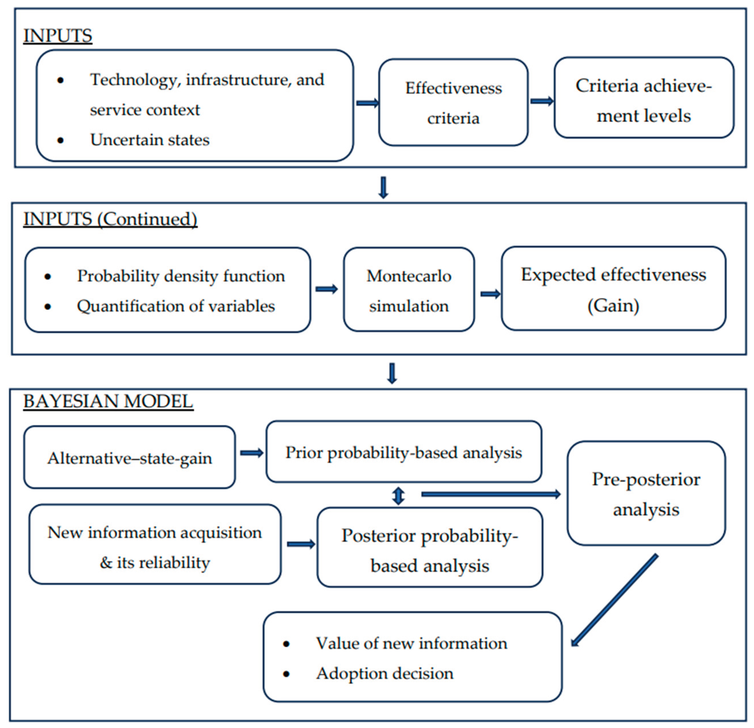
Figure 2.
Transformation of criteria achievement levels (Adapted from Reference 38).
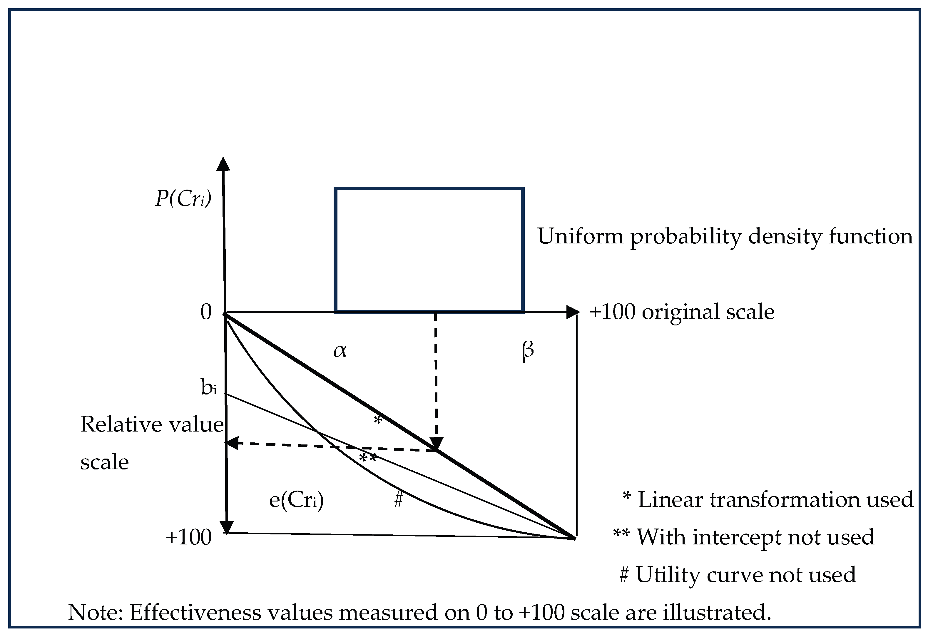
Figure 3.
Uniform probability distribution function.
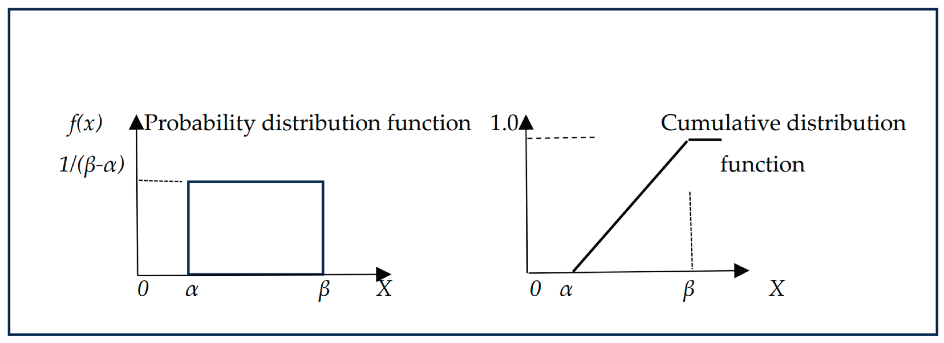
Figure 4.
Triangular probability distribution function.
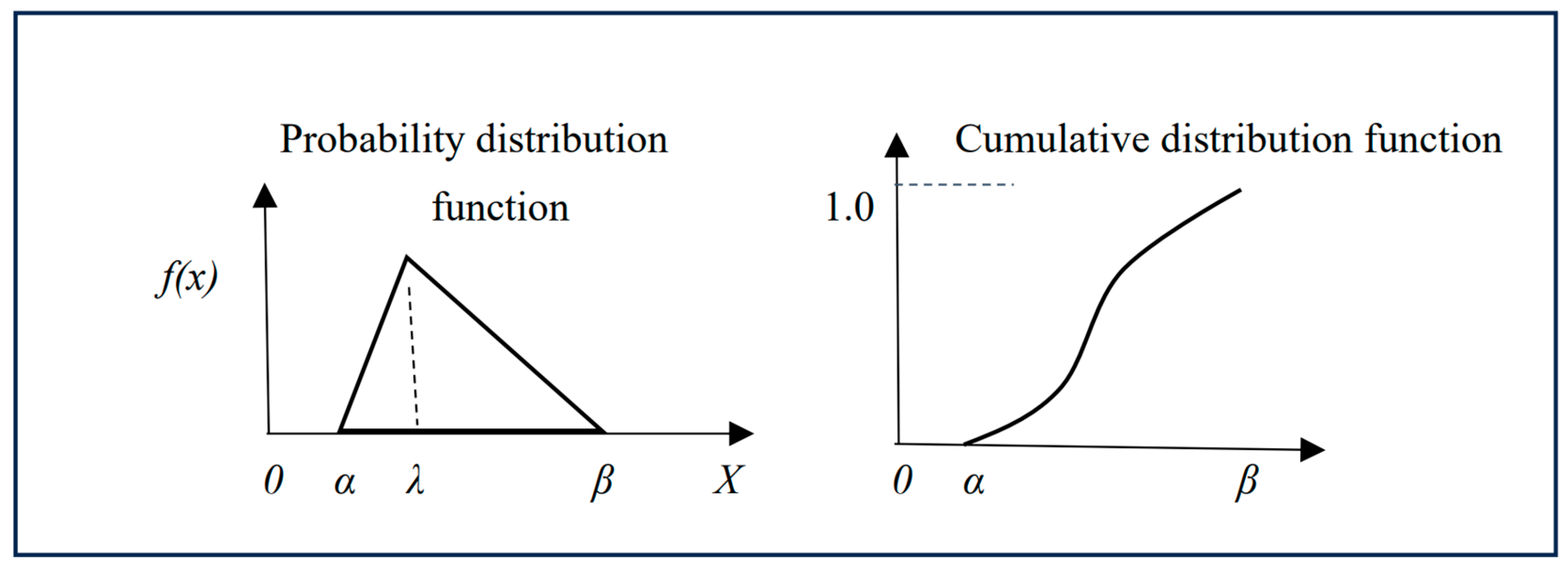
Figure 5.
Analysis based on prior probabilities.
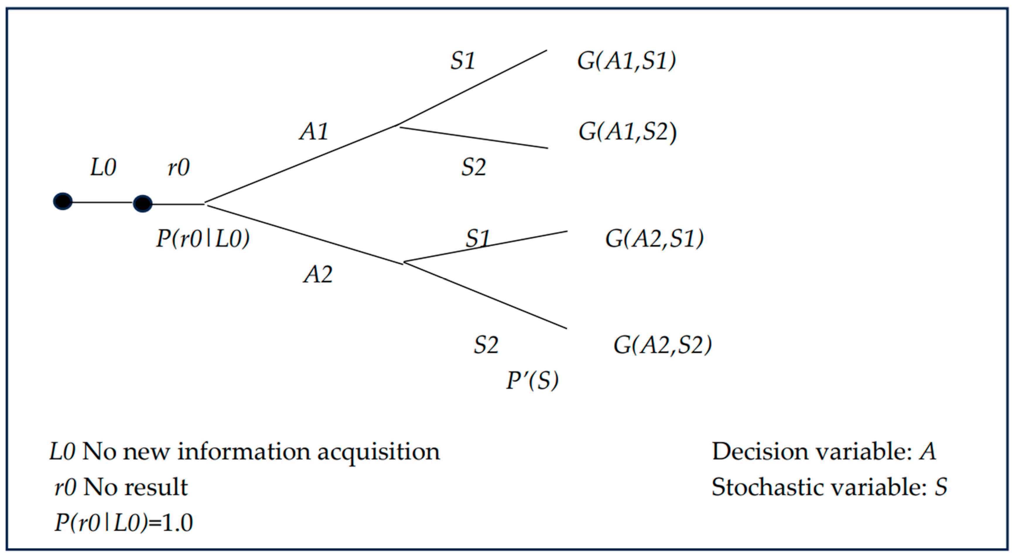
Figure 6.
Analysis based on posterior probabilities.
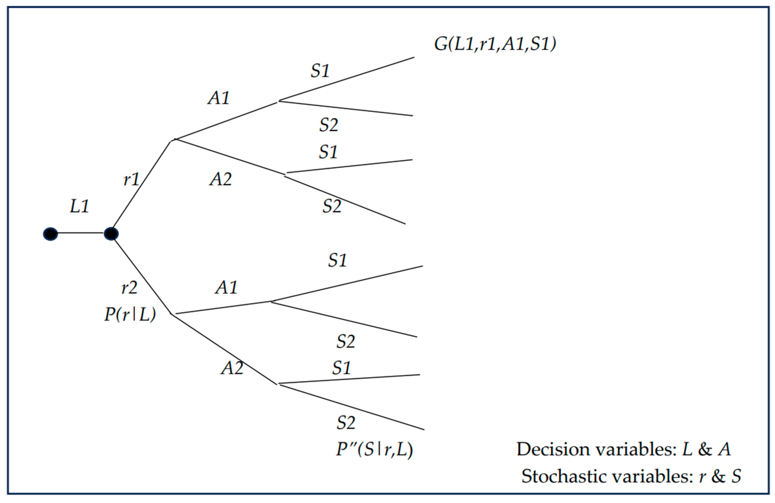
Figure 7.
Value of new information.
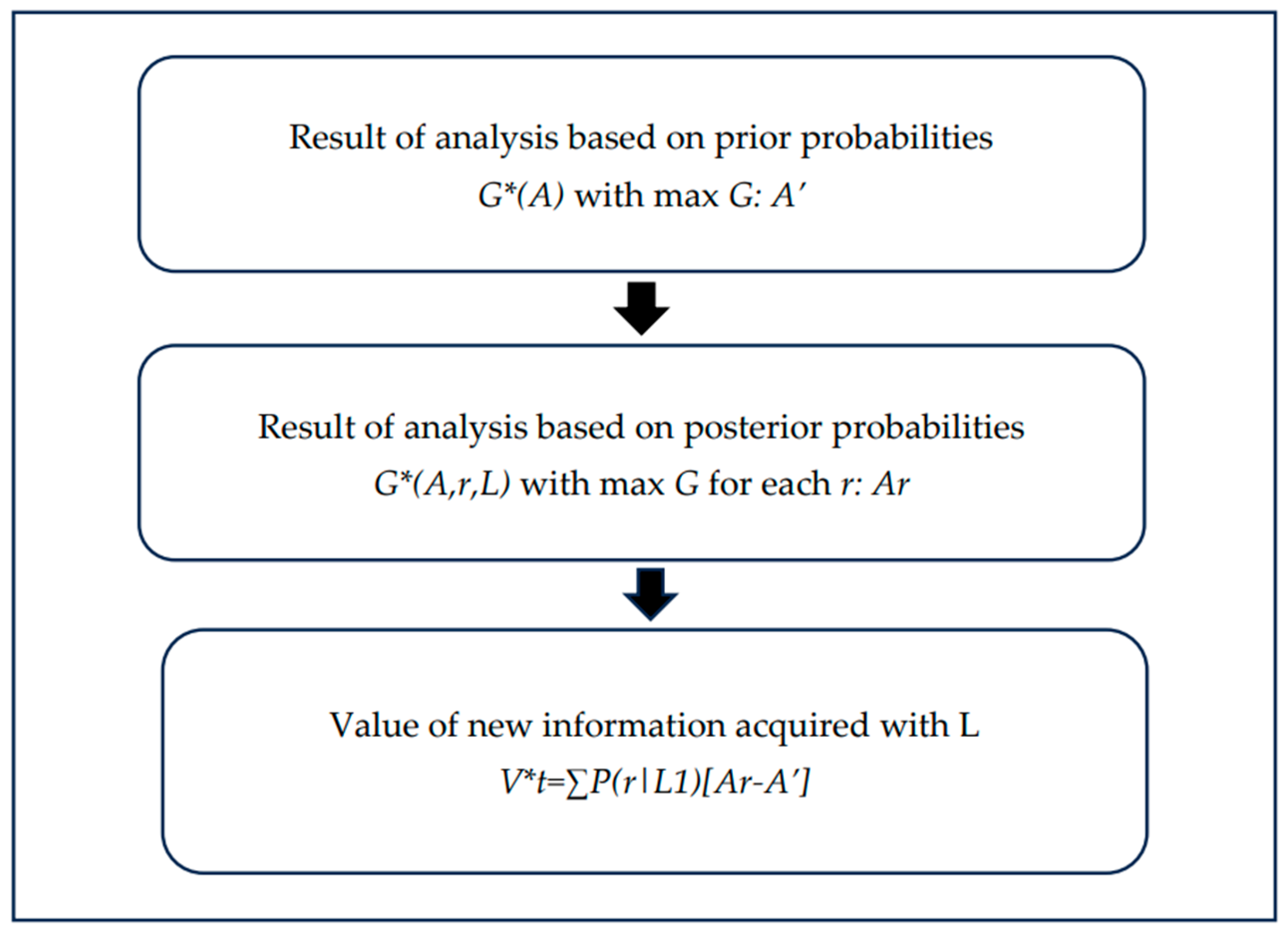
Figure 8.
The effect of favorable result new information on posterior probabilities.
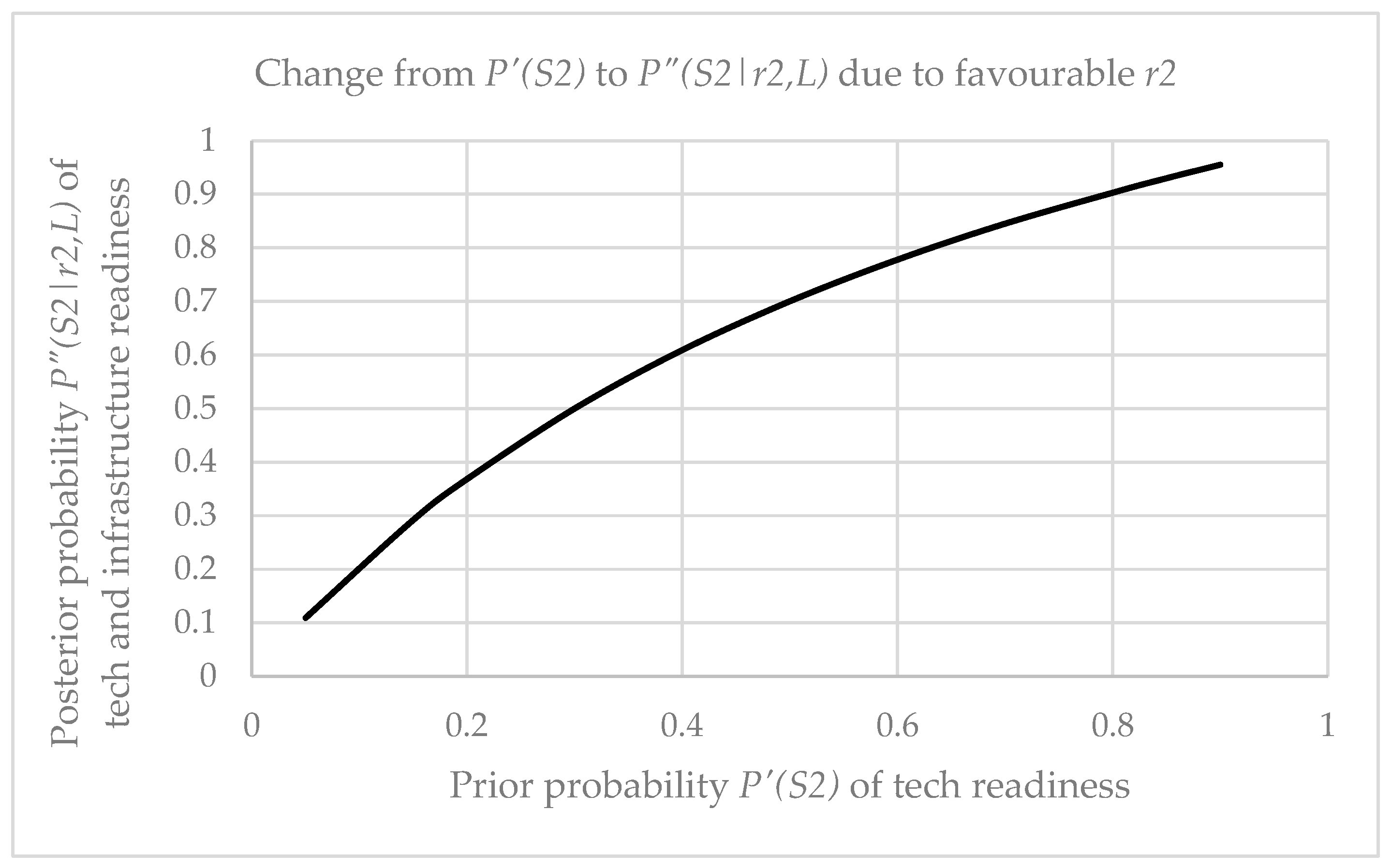
Figure 9.
Expected value of adopting CAV (includes value of new information) .
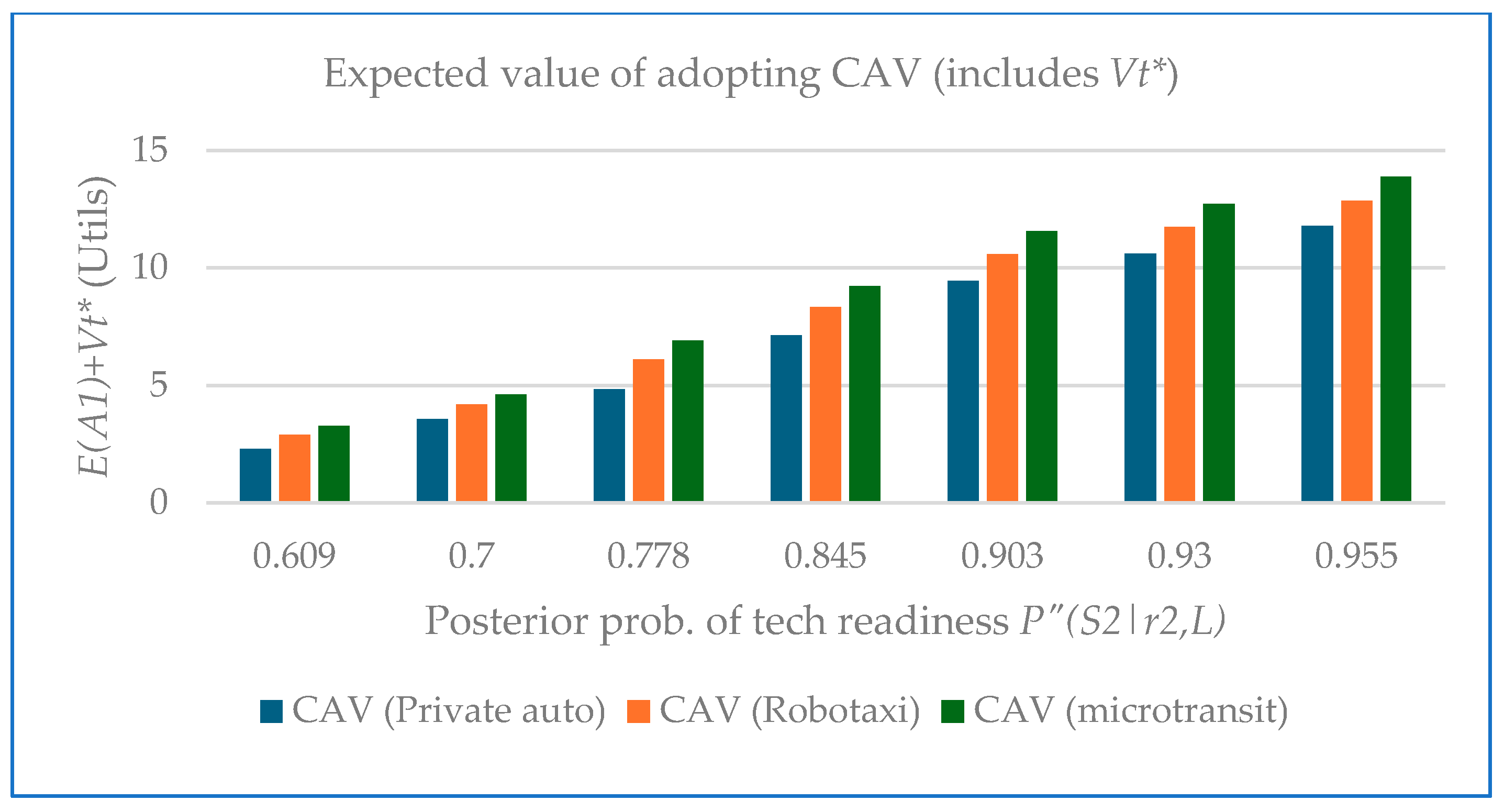
Figure 10.
Role of new information.
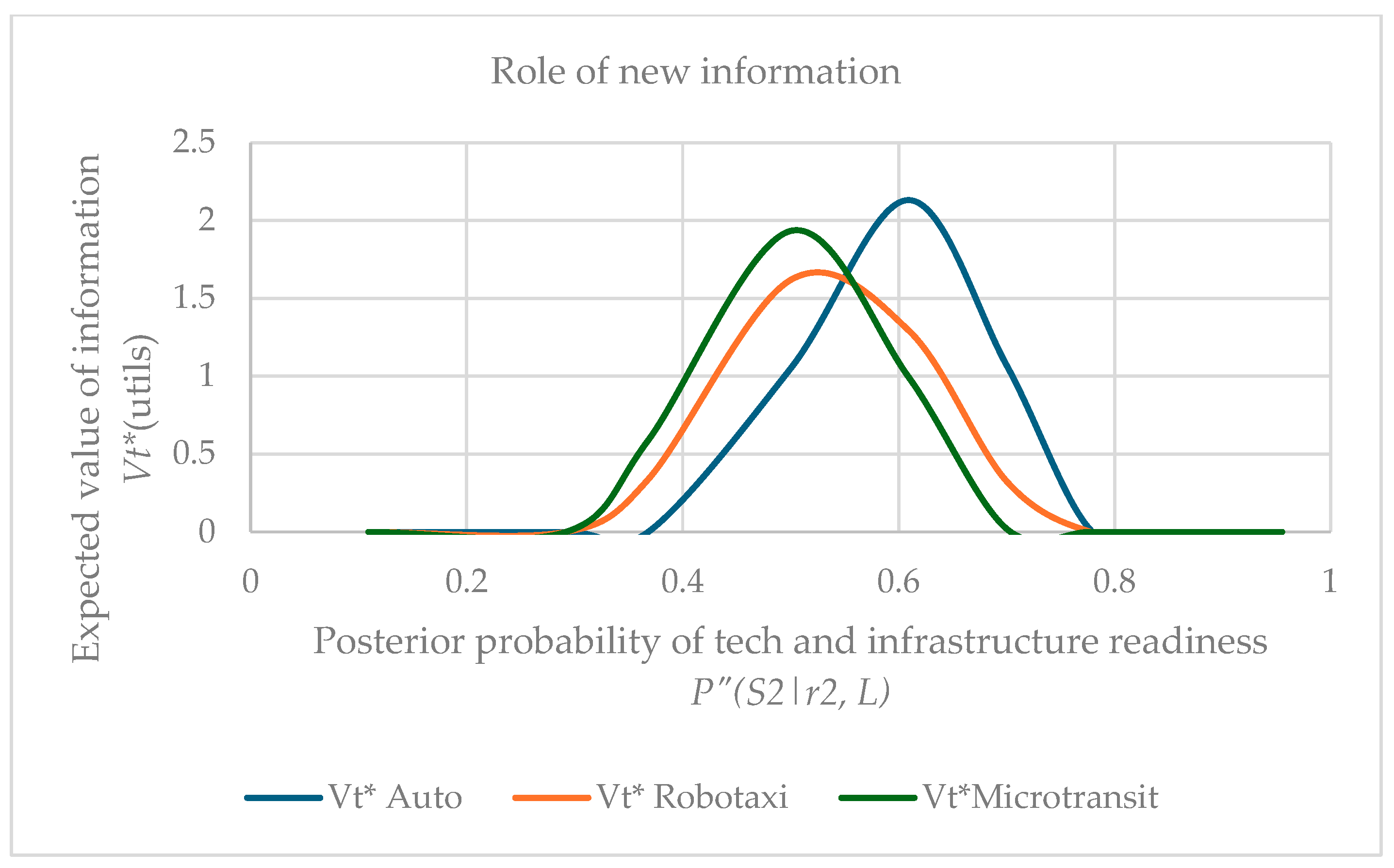
Figure 11.
Effect of reliability of new information on value of new information.
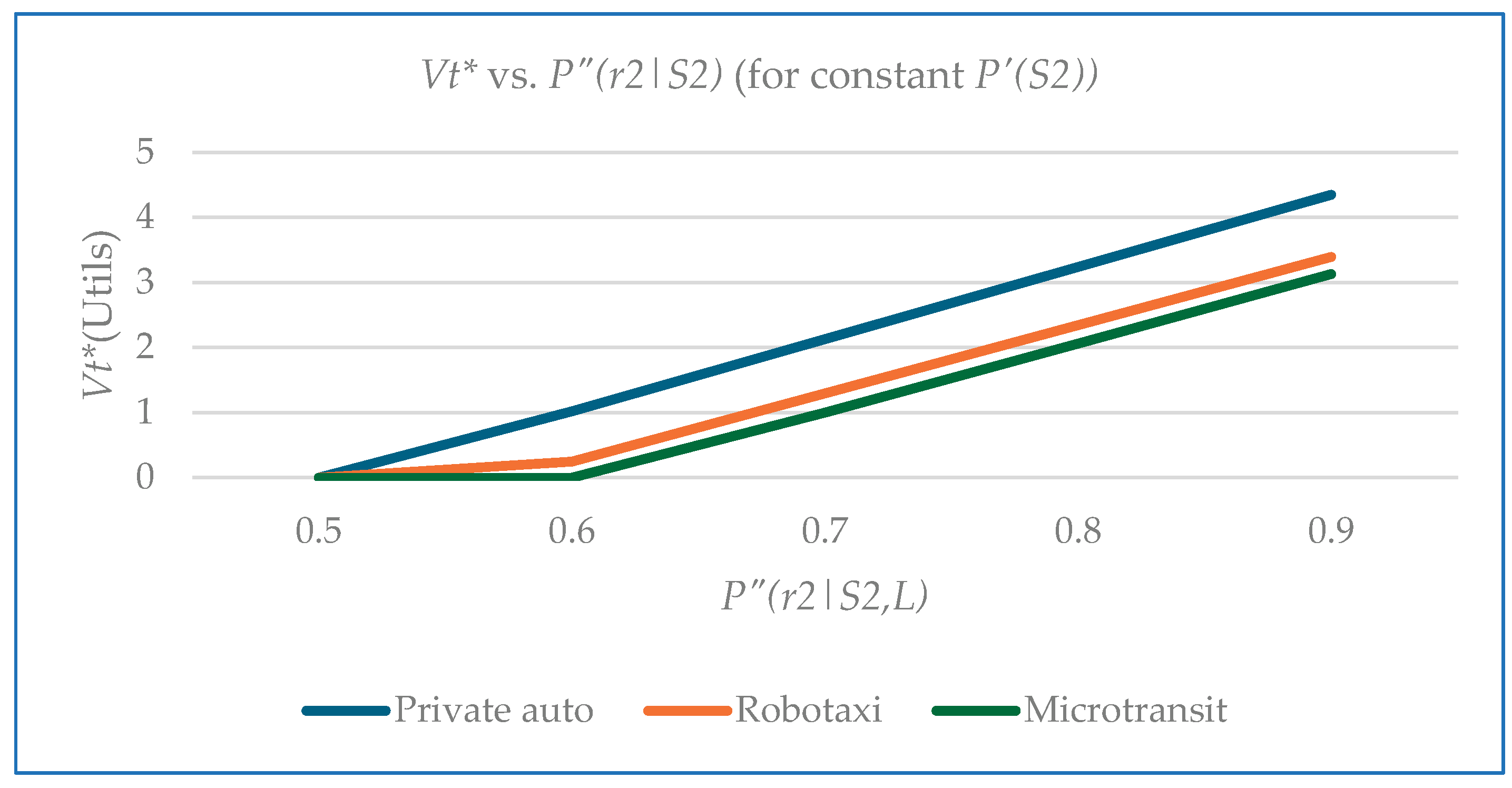

Table 1.
Variables for modelling the decision-making problem.
| Use cases (2030-2035 market context) | Decisions | Decision-makers | Uncertain States | Impacts (effects) |
| Personal passenger vehicle use |
A1: Purchase CAV A2: Do not purchase CAV |
Individual consumer |
S1: Uncertain. Low state of technology and infrastructure readiness S2: Uncertain, but higher state of technology & infrastructure readiness |
Multi-attribute utility of A-S combinations. |
| Robotaxi service |
A1: Invest in CAV fleet, infrastructure, operation & management system. A2: Do not. |
Corporate decision |
S1: Uncertain. Low state of technology & infrastructure readiness. Developing market potential. S2: Uncertain, but higher state of technology and infrastructure readiness. Promising market potential. |
Multi-attribute utility of A-S combinations. |
| CAV-based microtransit service |
A1: Invest in CAV fleet, infrastructure, operation & management system. A2: Do not. |
Public transit management decision. Corporate decision for private sector service. |
S1: Uncertain. Low state of technology & infrastructure readiness. Developing market potential. S2: Uncertain, but higher state of technology and infrastructure readiness. Promising market potential |
Multi-attribute utility of A-S combinations. |
Table 2.
Effectiveness criteria and criteria Weights.
| Criteria | Criteria weight | Normalized weight |
| Human factors-related collisions avoided User satisfaction Cr3 Socio-economic benefits Cr4 Environment Cr5 Tech unreliability Cr6 Effect on road users Cr7 Hacking, data security Cr8 Cost differential |
10 3 2 2 4 6 4 3 34 |
0.29 0.09 0.06 0.06 0.12 0.18 0.12 0.09 ~1.00 |
Table 3.
Effectiveness under S1: Level 4 CAV as a private vehicle (utils).
| Criteria |
S1 Effectiveness (-100 to +100 scale) |
S1 Expected effectiveness & St. Dev. based on triangular probability distribution |
S1 Expected effectiveness & St. Dev. based on uniform probability distribution |
S1 Weighted effectiveness (based on uniform probability distribution results and normalized weights) |
|
Cr1 Collisions avoided Cr2 User satisfaction Cr3 Socio-economic benefits Cr4 Environment Cr5 Tech unreliability Cr6 Effect on road users Cr7 Hacking, data security Cr8 Cost differential |
25 to 40 30 to 45 15 to 30 20 to 40 -25 to -50 -35 to -65 -25 to -50 -60 to -90 |
32.7 & 4.5 37.5 & 3.4 22.5 & 3.4 30.0 & 5.5 -50.5 & 6.2 -44.3 & 7.0 -38.3 & 5.7 -76.0 & 5.4 |
33.1&4.6 37.6 &4.7 22.6 &4.2 30.0 &7.1 -39.2&7.4 -50.4&9.0 -39.2&7.4 -75.4&9.2 |
9.6 3.4 1.4 1.8 -4.7 -9.1 -4.7 -6.8 -9.1 |
Table 4.
Effectiveness under S2: Level 4 CAV as a private vehicle (utils).
| Criteria |
S2 Effectiveness (-100 to +100 scale) |
S2 Expected effectiveness & St. Deviation based on triangular probability distribution |
S2 Expected effectiveness & St. Deviation based uniform probability distribution |
S2 Weighted effectiveness (based on uniform probability distribution results and normalized weights) |
|
Cr1 Collisions avoided Cr2 User satisfaction Cr3 Socio-economic benefits Cr4 Environment Cr5 Tech unreliability Cr6 Effect on road users Cr7 Hacking, data security Cr8 Cost differential |
40 to 70 30 to 45 20 to 40 20 to 40 0 to -25 0 to -30 0 to -20 -10 to -40 |
55.1 & 6.3 37.8 & 3.3 30.0 & 5.5 30.0 & 5.5 -12.3 & 5.1 -15.2 & 6.9 -10.7 & 4.6 -26.3 & 6.8 |
55.2 &9.8 37.8 &4.6 30.0 &7.1 30.0 &7.1 -12.6 &7.4 -15.6 &9.8 -10.8&6.9 -25.1&8.1 |
16.0 3.4 1.8 1.8 -2.5 -2.8 -1.3 -2.3 14.1 |
Table 5.
Effectiveness under S1: Level 4 CAV as a ride-hailing robotaxi (utils)
| Criteria |
S1 Effectiveness (-100 to +100 scale) |
S1 Expected effectiveness & St. Dev. based on triangular probability distribution |
S1 Expected effectiveness & St. Dev. based on uniform probability distribution |
S1 Weighted effectiveness (based on uniform probability distribution results and normalized weights |
|
Cr1 Collisions avoided Cr2 User satisfaction Cr3 Socio-economic benefits Cr4 Environment Cr5 Tech unreliability Cr6 Effect on road users Cr7 Hacking, data security Cr8 Cost differential |
25 to 40 25 to 45 15 to 30 20 to 40 -25 to -50 -30 to -60 -25 to -50 -50 to -80 |
32.7 & 4.5 37.5 & 4.5 22.6 & 3.1 30.0 & 5.5 -38.3 & 5.7 -44.3 & 7.0 -38.3 & 5.7 -65.3 & 7.5 |
33.1&4.6 33.3 &4.6 22.8 &4.2 30.0 &7.1 -39.2&7.4 -43.3&9.6 -39.2&7.4 -66.7&9.8 |
9.6 3.0 1.4 1.8 -4.7 -7.8 -4.7 -6.0 -7.4 |
Table 6.
Effectiveness under S2: Level 4 (CAV as a ride hailing robotaxi (utils).
| Criteria |
S2 Effectiveness (-100 to +100 scale) |
S2 Expected effectiveness & St. Deviation based on triangular probability distribution |
S2 Expected effectiveness & St. Deviation based uniform probability distribution |
S2 Weighted effectiveness (based on uniform probability distribution results and normalized weights) |
|
Cr1 Collisions avoided Cr2 User satisfaction Cr3 Socio-economic benefits Cr4 Environment Cr5 Tech unreliability Cr6 Effect on road users Cr7 Hacking, data security Cr8 Cost differential |
40 to 70 30 to 45 20 to 40 20 to 40 0 to -25 0 to -30 0 to -30 -10 to -30 |
55.1 & 6.3 37.2 & 3.1 30.0 & 5.5 30.0 & 5.5 -12.2 & 5.1 -15.2 & 6.9 -15.0 & 6.8 -20.9 & 4.0 |
55.2 &9.8 37.7 &4.1 30.0 &7.1 30.0 &7.1 -12.7 &7.1 -15.6 &9.8 -15.0&8.6 -20.4&5.9 |
16.0 3.4 1.8 1.8 -1.5 -2.8 -1.8 -1.8 15.1 |
Table 7.
Effectiveness under S1: Level 4 CAV used as a Microtransit Vehicle (utils).
| Criteria |
S1 Effectiveness (-100 to +100 scale) |
S1 Expected effectiveness & St. Dev. based on triangular probability distribution |
S1 Expected effectiveness & St. Dev. based on uniform probability distribution |
S1 Weighted effectiveness (based on uniform probability distribution results and normalized weights) |
|
Cr1 Collisions avoided Cr2 User satisfaction Cr3 Socio-economic benefits Cr4 Environment Cr5 Tech unreliability Cr6 Effect on road users Cr7 Hacking, data security Cr8 Cost differential |
25 to 40 25 to 40 20 to 40 20 to 40 -25 to -50 -30 to -60 -25 to -50 -50 to -80 |
32.7 & 4.5 32.7 & 4.5 30.0 & 5.5 30.0 & 5.5 -38.3 & 5.7 -44.3 & 7.0 -38.3 & 5.7 -65.3 & 7.5 |
33.1&4.6 33.3 &4.6 30.0 &7.1 30.0 &7.1 -39.2&7.4 -43.3&9.6 -39.2&7.4 -66.7&9.8 |
9.6 3.0 1.8 1.8 -4.7 -7.8 -4.7 -6.0 -7.0 |
Table 8.
Effectiveness Under S2: Level 4 CAV as a Microtransit Vehicle (utils).
| Criteria |
S2 Effectiveness (-100 to +100 scale) |
S2 Expected effectiveness & St. Deviation based on triangular probability distribution |
S2 Expected effectiveness & St. Deviation based uniform probability distribution |
S2 Weighted effectiveness (based on uniform probability distribution results and normalized weights) |
|
Cr1 Collisions avoided Cr2 User satisfaction Cr3 Socio-economic benefits Cr4 Environment Cr5 Tech unreliability Cr6 Effect on road users Cr7 Hacking, data security Cr8 Cost differential |
40 to 70 25 to 40 20 to 40 20 to 40 0 to -17.5 0 to -30 0 to -20 0 to -30 |
55.1 & 6.3 32.7 & 4.5 30.0 & 5.5 30.0 & 5.5 -8.6 & 4.5 -15.2 & 6.9 -10.7 & 4.6 -14.9 & 5.8 |
55.2 &9.8 33.3 &4.6 30.0 &7.1 30.0 &7.1 -8.3 &6.4 -15.6 &9.8 -10.8&6.9 -14.4 &9.4 |
16.0 3.0 1.8 1.8 -1.0 -2.8 -1.3 -1.3 16.2 |
Table 9.
Bayesian prediction of private auto CAV adoption (A1 adopt, A2 do not adopt).
| Prior prob. P’(S1) & P’(S2) |
Conditional prob. P(r1|S1)&P(r2|S1) | Selected conditional prob. P(r1|S2)& P(r2|S2) | Selected Posterior prob. P”(S1|r2,L)& P”(S2|r2,L) |
Gain (utils) G(A1,S1) &G(A2,S1) |
Gain (utils) G(A1,S2) &G(A2,S2) | Value of new information Vt*(utils) | Choice of A & E(A) (utils) | Interpretation of Results |
| 0.95& 0.05 to 0.80&0.20 |
0.7&0.30 | 0.3&0.70 | 0.891&0.109 To 0.632&0.368 |
-9.1&0 | 14.1&0 | 0 | A2& 0 | CAV will not be adopted. New information will not change the choice. |
| 0.70&0.30 | 0.7&0.30 | 0.3&0.70 | 0.500&0.500 | -9.1&0 | 14.1&0 | 1.05 | A2& 0 | CAV will not be adopted. But new information can reduce risk. |
| 0.60&0.40 | 0.7&0.30 | 0.3&0.70 | 0.391&0.609 | -9.1&0 | 14.1&0 | 2.13 | A1& 0.18 | CAV will be adopted, subject to new information for risk reduction. |
| 0.50&0.50 | 0.7&0.30 | 0.3&0.70 | 0.300&0.700 | -9.1&0 | 14.1&0 | 1.07 | A1& 2.50 | CAV will be adopted, subject to new information for risk reduction. |
| 0.40&0.60 | 0.7&0.30 | 0.3&0.70 | 0.222&0.778 | -9.1&0 | 14.1&0 | 0.01 | A1& 4.82 | CAV will be adopted, subject to new information for risk reduction. |
| 0.30&0.70 | 0.7&0.30 | 0.3&0.70 | 0.155&0.845 | -9.1&0 | 14.1&0 | 0 | A1& 7.14 | CAV will be adopted. No need for new information. |
| 0.20&0.80 | 0.7&0.30 | 0.3&0.70 | 0.097&0.903 | -9.1&0 | 14.1&0 | 0 | A1& 9.46 | CAV will be adopted. No need for new information. |
| 0.15&0.85 | 0.7&0.30 | 0.3&0.70 | 0.070&0.930 | -9.1&0 | 14.1&0 | 0 | A1& 10.62 | CAV will be adopted. No need for new information. |
| 0.10&0.90 | 0.7&0.30 | 0.3&0.70 | 0.045&0.955 | -.9.1&0 | 14.1&0 | 0 | A1& 11.78 | CAV will be adopted. No need for new information. |
Table 10.
Bayesian prediction of robotaxi CAV adoption (A1 adopt, A2 do not adopt).
| Prior prob. P’(S1) & P’(S2) |
Conditional prob. P(r1|S1)&P(r2|S1) | Selected conditional prob. P(r1|S2)& P(r2|S2) | Selected Posterior prob. P”(S1|r2,L)& P”(S2|r2,L) |
Gain (utils) G(A1,S1) &G(A2,S1) | Gain (utils) G(A1,S2) &G(A2,S2) | Value of new information Vt*(utils) | Choice of A & E(A) (utils) | Interpretation of Results |
| 0.95& 0.05 to 0.85&0.15 |
0.7&0.30 | 0.3&0.70 | 0.891&0.109 to 0.708&0.292 |
-7.4&0 | 15.1&0 | 0 to 0 |
A2& 0 | CAV will not be adopted. New information will not change the choice. |
| 0.80&0.20 | 0.70&0.30 | 0.3&0.70 | 0.632&0.368 | -7.4&0 | 15.1&0 | 0.338 | A2&0 | CAV will not be adopted. But new information can reduce risk. |
| 0.70&0.30 | 0.7&0.30 | 0.3&0.70 | 0.500&0.500 | -7.4&0 | 15.1&0 | 1.617 | A2& 0 | CAV will not be adopted. But new information can reduce risk. |
| 0.60&0.40 | 0.7&0.30 | 0.3&0.70 | 0.391&0.609 | -7.4&0 | 15.1&0 | 1.296 | A1& 2.896 | CAV will be adopted, subject to new information for risk reduction. |
| 0.50&0.50 | 0.7&0.30 | 0.3&0.70 | 0.300&0.700 | -7.4&0 | 15.1&0 | 0.325 | A1&3.85 | CAV will be adopted, subject to new information for risk reduction. |
| 0.40&0.60 | 0.7&0.30 | 0.3&0.70 | 0.222&0.778 | -7.4&0 | 15.1&0 | 0 | A1& 6.1 | CAV will be adopted. No need for new information. |
| 0.30&0.70 | 0.7&0.30 | 0.3&0.70 | 0.155&0.845 | -7.4&0 | 15.1&0 | 0 | A1& 8.35 | CAV will be adopted. No need for new information. |
| 0.20&0.80 | 0.7&0.30 | 0.3&0.70 | 0.097&0.903 | -7.4&0 | 15.1&0 | 0 | A1& 10.6 | CAV will be adopted. No need for new information. |
| 0.15&0.85 | 0.7&0.30 | 0.3&0.70 | 0.070&0.930 | -7.4&0 | 15.1&0 | 0 | A1& 11.725 | CAV will be adopted. No need for new information. |
| 0.10&0.90 | 0.7&0.30 | 0.3&0.70 | 0.045&0.955 | -7.4&0 | 15.1&0 | 0 | A1&12.85 | CAV will be adopted. No need for new information. |
Table 11.
Bayesian prediction of microtransit CAV adoption (A1 adopt, A2 do not adopt).
| Prior prob. P’(S1) & P’(S2) |
Conditional prob. P(r1|S1)& P(r2|S1) | Conditional prob. P(r1|S2)& P(r2|S2) | Selected Posterior prob. P”(S1|r2,L)& P”(S2|r2,L) |
Gain (utils) G(A1,S1) &G(A2,S1) | Gain (utils) G(A1,S2) &G(A2,S2) | Value of new information Vt*(utils) | Choice of A & E(A) (utils) | Interpretation of Results |
| 0.95& 0.05 to 0.85&0.15 |
0.7&0.30 | 0.3&0.70 | 0.891&0.109 to 0.708&0.292 |
-7.0&0 | 16.2&0 | 0 to 0 |
A2& 0 | CAV will not be adopted. New information will not change the choice. |
| 0.80&0.20 | 0.70&0.30 | 0.3&0.70 | 0.632&0.368 | -7.0&0 | 16.2&0 | 0.588 | A2&0 | CAV will not be adopted. But new information can reduce risk. |
| 0.70&0.30 | 0.7&0.30 | 0.3&0.70 | 0.500&0.500 | -7.0&0 | 16.2&0 | 1.932 | A2& 0 | CAV will not be adopted. But new information can reduce risk. |
| 0.60&0.40 | 0.7&0.30 | 0.3&0.70 | 0.391&0.609 | -7.0&0 | 16.2&0 | 0.996 | A1& 2.28 | CAV will be adopted, subject to new information for risk reduction. |
| 0.50&0.50 | 0.7&0.30 | 0.3&0.70 | 0.300&0.700 | -7.0&0 | 16.2&0 | 0.02 | A1& 4.60 | CAV will be adopted, subject to new information for risk reduction. |
| 0.40&0.60 | 0.7&0.30 | 0.3&0.70 | 0.222&0.778 | -7.0&0 | 16.2&0 | 0 | A1& 6.92 | CAV will be adopted. No need for new information. |
| 0.30&0.70 | 0.7&0.30 | 0.3&0.70 | 0.155&0.845 | -7.0&0 | 16.2&0 | 0 | A1& 9.24 | CAV will be adopted. No need for new information. |
| 0.20&0.80 | 0.7&0.30 | 0.3&0.70 | 0.097&0.903 | -7.0&0 | 16.2&0 | 0 | A1& 11.56 | CAV will be adopted. No need for new information. |
| 0.15&0.85 | 0.7&0.30 | 0.3&0.70 | 0.070&0.930 | -7.0&0 | 16.2&0 | 0 | A1& 12.72 | CAV will be adopted. No need for new information. |
| 0.10&0.90 | 0.7&0.30 | 0.3&0.70 | 0.045&0.955 | -7.0&0 | 16.2&0 | 0 | A1&13.88 | CAV will be adopted. No need for new information. |
Table 12.
Effect of conditional probabilities on Vt*.
| P(r2|S2,L) | P’(S1)&P’(S2) | P”(S2|r2,L) | Private auto Vt* | Robotaxi Vt* | Microtransit Vt* |
| 0.5 | 0.6&0.4 | 0.40 | 0 | 0 | 0 |
| 0.6 | 0.6&0.4 | 0.50 | 1.02 | 0.248 | 0 |
| 0.7 | 0.6&0.4 | 0.609 | 2.13 | 1.296 | 1 |
| 0.8 | 0.6&0.4 | 0.727 | 3.24 | 2.344 | 2.06 |
| 0.9 | 0.6&0.4 | 0.857 | 4.35 | 3.392 | 3.13 |
Disclaimer/Publisher’s Note: The statements, opinions and data contained in all publications are solely those of the individual author(s) and contributor(s) and not of MDPI and/or the editor(s). MDPI and/or the editor(s) disclaim responsibility for any injury to people or property resulting from any ideas, methods, instructions or products referred to in the content. |
© 2025 by the authors. Licensee MDPI, Basel, Switzerland. This article is an open access article distributed under the terms and conditions of the Creative Commons Attribution (CC BY) license (http://creativecommons.org/licenses/by/4.0/).
Copyright: This open access article is published under a Creative Commons CC BY 4.0 license, which permit the free download, distribution, and reuse, provided that the author and preprint are cited in any reuse.


