
Submitted:
30 June 2025
Posted:
01 July 2025
You are already at the latest version
Abstract
In the prairie provinces of Western Canada, including Saskatchewan, many farms lack access to potable, healthy water and rely on dugouts for their water supply. Dugouts are artificial ponds or reservoirs that collect and store water, often from rain or snowmelt, for agricultural and livestock use. Dugouts contain, in some cases, high sulfate con-taminants that impact livestock watering. To clean these kinds of waters, a full factorial design study with eleven experiments was carried out to evaluate and optimize key nanofiltration membrane operating conditions, such as Trans-Membrane Pressure (TMP), Crossflow Velocity (CVF), and magnesium sulfate (MgSO4) concentration, fo-cusing on their impact on rejection rates and permeate flux. With optimal conditions of a TMP of 9 bar and a CFV of 0.65 m/s, the nanofiltration (NF90) membrane achieved a sulfate rejection of 90% and a permeate flux of 127 LMH, with CFV identified as the most significant factor influencing the operation of the membrane at all concentrations. Analysis of Variance (ANOVA) confirmed the statistical significance of the polynomial regression models, with a 95% confidence interval (CI). The membrane's rejection data and flux regression models yield a strong fit to the data, with a correlation coefficient exceeding 99%. Using the experimental dataset, two machine learning algorithms— Decision Tree (DT) and Random Forest (RF) — were employed to predict the permeate flux. The RF model demonstrated excellent predictive performance across all data sets, achieving a root mean square error (RMSE) of 3.98 and a coefficient of determination (R²) of 0.99. These findings highlight the potential of machine learning for predicting effec-tive sulphated water treatment.
Keywords:
Full Factorial
; Dugouts
; Nanofiltration 90 polymeric membrane
; Sulfated water
; Modelling
; Random Forest
; Decision Tree
1. Introduction
There is a plentiful surface and groundwater supply in western Canada, but much of it contains high dissolved solutes. According to recent data published by the Saskatchewan Ministry of Agriculture, over 52% of the 712 ground and surface water samples tested in 2018 and 2019 had sulfate concentrations above 1000 mg/L [1]. According to the Nutrient Requirements of Beef Cattle (NRC) [2]. Based on the available data, water provided to cattle on high-forage diets should not have sulphate levels higher than 2500 mg/L. Water consumption by cattle starts to decrease when sulfate levels exceed 2000 mg/L [3,4] and declines further at higher concentrations [5]. For 7 days, high sulfate levels in water have reduced feed intake and lowered body weight gain [4,5]. One study found that when sulphate levels in water exceeded 3000 mg/L, cattle significantly reduced their water intake. This effect was more pronounced with magnesium sulfate than with sodium sulfate. As the concentration of magnesium sulfate increased, average daily water consumption dropped from about 40.1 L per day to just 12.8 L at 4500 mg/L sulfate. In contrast, the reduction with sodium sulfate was less severe [6].
Similarly, Morris et al. [7] found out that magnesium sulfate has a more substantial laxative impact than sodium sulfate. The latter is less completely absorbed, significantly impacting the osmolality of the intestinal contents. Two studies have highlighted that consuming large amounts of magnesium sulfate can lead to various health issues, such as diarrhea, dehydration, catharsis, and alterations in the levels of methemoglobin and sulfhemoglobin in both humans and animals, in addition to gastric discomfort, and a laxative effect [8,9]. Darbi et al. [10] studied sulfated waters, choosing magnesium sulfate over calcium sulfate because the latter is slightly soluble in water at high concentrations and can form a cloudy or turbid solution. This high-turbidity or cloudy solution can lead to scaling when using a resin in ion-exchange or membrane filtration, and negatively impact its performance. According to Nariyan et al. [11], elevated levels of sulfate in discharged water can raise the salinity of the receiving water body, such as a lake. The World Health Organization (WHO) recommends a maximum sulfate concentration of 500 mg/L in drinking water, but concentrations in the prairies often exceed the guidelines.
Different primary water treatment systems that remove sulfate from water include chemical precipitation, biological sulfate reduction, ion exchange, and evaporation [12]. Still, these are not fit for dugouts because of their high cost. Membrane technologies have become crucial in environmental protection, particularly for reducing pollution and enabling the treatment of sulfated water. Nanofiltration (NF) and reverse osmosis (RO) membranes are widely used in water and wastewater treatment, as they produce high-quality water [13]. NF membranes offer several advantages over ultrafiltration (UF) and RO membranes. For example, they can operate at lower pressures than RO membranes while still achieving higher rejection of multivalent salts and other molecular compounds than UF [14].
Although there are a few publications on sulfate removal from surface water, several studies have focused on sulfate removal from wastewater. Reis et al. [15] investigated the treatment of sulfuric acid plant wastewater using NF membranes. Their research studied the impact of key operational parameters, including feed pH, applied pressure, and permeate recovery rate. They used an NF90 membrane and real wastewater from a sulfuric acid production facility. Under optimal conditions, a pH of 2 and an applied pressure of 10 bar, the NF90 membrane achieved a sulfate rejection rate of 94%. In a recent study published by Jadhav et al. [16], sulphate removal from water using NF was examined. They utilized NF270 and NF90 membranes to eliminate various contaminants, including fluoride, arsenic, sulfate, and nitrate, from ultra-pure water mixed with these contaminants. They found that both membranes were highly effective in separating sulfate, with the NF90 membrane achieving a rejection rate of 95%.
In comparison, the NF270 membrane had a rejection rate of approximately 90%, irrespective of the operating conditions. Krieg et al. [17] evaluated the sulfate rejection capabilities of the NF90 membrane and compared it with the NF70 membrane using both single sulfate salts and binary sulfate salt mixtures. The results indicated that both membranes were similarly effective in rejecting sulfate, achieving over 90% rejection.
Machine Learning (ML) based modeling is among the most widely used and effective options. ML can be utilized to design, analyze, and predict the performance of membrane technologies, reducing the need for expensive and time-intensive experimental research and pilot studies [18,19]. ML has been increasingly utilized in membrane-based water treatment in recent years, particularly for predicting the permeate flux [20]. Among ML models, artificial neural networks (ANNs) are the most widely used in membrane-based water treatment. Our research group applied ANN to model flux decline in oily wastewater, achieving impressive accuracy with a Mean Squared Error (MSE) of 0.004 and a correlation coefficient (R) of 0.99, reflecting an excellent match between predicted and actual results [21]. We also used ANN predictions for produced water treatment, which were highly accurate, achieving a coefficient of determination R² of 99% and an MSE of 0.07 [22]. In another study, Schmitt et al. [23] demonstrated that ANN provided accurate predictions of membrane fouling, with a satisfactory performance marked by an R² of 85%.
This study aims to determine the best operating conditions for the NF90 membrane to maximize sulfate rejection and permeate flux. A factorial design approach was used, followed by statistical Analysis Of Variance (ANOVA) to identify the optimal levels for each influencing parameter. Two machine learning models, DT and RF, were developed to create a framework for predicting system behaviour under various conditions. These models were also applied to forecast the decline in flux over time.
2. Methodology of the Experimental
2.1. General Procedure
Filtration experiments were conducted using a system purchased from Sterlitech Corp. (Auburn, WA, USA). A simple diagram of the setup is shown in Figure 1. The feed solution is stored in a 5-gallon (18.9 L) stainless-steel tank. The feed solution is pumped into a membrane cell with an effective membrane area of 42 cm² (6.5 in²), using a Hydra cell C pump, and an Emerson Controller to maintain a given speed. Several valves, provided by Swagelok Co. (Saskatoon, Canada), ensure safety and monitor the pressure and flow. Pressure sensors (0 to 69 bar), with an accuracy of ±0.3% %, are placed on both sides of the membrane cell, and their readings are displayed digitally.
The rejection solution is sent through a brine or concentration control valve to a Dwyer (Michigan City, IN, USA) digital flow meter (0 to 6.8 L/min), with an accuracy of ±1% %. The rejected flow is returned to the feed tank to maintain a constant concentration. The filtered permeate is collected in a beaker on a Mettler Toledo (Mississauga, ON, Canada) MS4002S mass balance (up to 4,200 g), with a standard deviation of 0.01g for repeated measurements. This mass balance is connected to a computer that automatically records and displays the weights.
The permeate weight is automatically recorded every 15 seconds in intervals through a USB connection to a computer. All experiments were carried out for approximately 1.5 hours each. The feed pressure and crossflow were controlled separately using bypass and brine control valves and a variable frequency drive (VFD). The bypass valve was closed while the brine or concentration valve was open, and the pump circulated the feed before the tests began. The filtration system was cleaned with deionized (DI) water, and a sample was taken to measure the electrical conductivity (EC), which needed to be between 0.1 and 5 µS/cm to minimize errors. Each membrane was soaked overnight in Deionized water (DI) before being installed in the filtration cell. The parameters and units used in the measurements are presented in Table 1.
2.2. Materials and Equipment
The commercial membrane, NF90, used in this study (Table 2) was purchased from Sterlitech Corp., after a comprehensive literature survey. Magnesium sulfate (≥99%) was purchased from Sigma-Aldrich and used as received for the feed preparation. Ultrapure deionized (DI) water, with very low organic content and minimal microorganisms, was produced using a reverse osmosis unit and a UV water purification system from Millipore Sigma (Oakville, ON, Canada). Pure DI water with a conductivity of 0.01 (µS/cm) was used to prepare the solutions at the desired concentrations of MgSO4 and for cleaning the filtration system before and after the treatment process. A Hanna (Laval, Quebec) device (HI 4522) was used to measure the EC of aqueous solutions (feed and permeate), while a Horiba F-55 benchtop meter (Burlington, ON, Canada) was used to measure the pH. For each experiment, a tank volume of 18.9 litres of MgSO4 solution was prepared by dissolving specific amounts of the salt into 1.5 litres of DI water, blending for 2-3 minutes, and repeating the process until the required total volume was obtained. The feed was measured before each run, and permeate was measured across various parameters.
At least duplicate samples were taken for each analysis, and the average values were used for data analysis. The membrane sulphate rejection performance was determined using the following Equation (1):
Cf and Cp represent the sulfate content in the feed and permeate, respectively, measured in mg/L. J represents the permeate flux (L/m² h) or (LMH) of a membrane by using Equation (2):
where V is the volume of permeate in (L), A is the membrane area (m²), and Δt is the time interval (h). The factorial design was utilized to analyze the responses through a quadratic polynomial regression model, Equation (3), which fits and optimizes the experimental data:
In this Equation, Yk represents the predicted response, where (k=1), Y1 is used as the membrane permeate flux. The variables (xi=1,2,3) correspond to the selected factors, where x1 is TMP, x2 is CFV, and x3 is MgSO4 concentration. While b0 is the constant coefficient, Se is the statistical error residual, and bi, bij, and bii represent the different types of regression coefficients (linear, interactional, and quadratic), respectively.
3. Experimental Design Based on Full Factorial and Modeling
The initial step in designing a robust study is determining the relationships between the parameters that influence the membrane operation. The rejection rate was the most critical parameter in optimizing membrane design. Rejection rates and permeate flux are influenced by several factors, including fouling, which depends on variables such as initial MgSO4 concentration [24,25,26], CFV [27,28], and TMP [29,30]. This study employed a full factorial design to address the complexity and numerous variables involved, thereby reducing the number of experiments required while maintaining statistical validity. This approach saves significant time, labor, and financial resources compared to exhaustive experimental studies. Additionally, machine learning (ML) was used to assess the model's accuracy and predictions against experimental data. Dansawad et al. [19] noted that RF and DT are less commonly applied in this area, highlighting a need for their application.
3.1. Full Factorial
Minitab 21 (State College, PA, USA ), a comprehensive software for data analysis and process improvement, was applied to analyze, visualize, and predict experimental data, enabling the development of a quadratic regression model to estimate response values. Specifically, a 2K full factorial approach was used in this study to evaluate the effects of three main independent variables: TMP, CFV, and concentration of MgSO4 on membrane performance. Other factors, such as pH and temperature (25±1°C), were kept constant throughout the experiments. These variables were selected due to their frequent mention in the literature as crucial for optimizing membrane processes. Each independent variable was tested at three levels: low (-1), middle (0), and high (+1), as shown in Table 3, allowing for a comprehensive analysis of how operating conditions interact. A total of 11 experimental runs were conducted to create a quadratic regression model, which included eight runs and three center points. Center points at different experiment stages were included to check for stability and potential curvature in the data [31]. The experiments were conducted randomly to reduce possible biases or errors in the results [32], and the ranges are established based on theory, equipment capabilities, and cost considerations. Table 3 details the coded levels for each independent variable used in the study.
3.2. Machine Learning Algorithms
Two machine learning algorithms, Decision Trees (DT) and Random Forest (RF), were selected based on their proven effectiveness and consistent use in predicting data, as well as their application in improving membrane separation performance for water treatment in various research studies. This selection was informed by extensive literature highlighting the predictive success of these models, ensuring a robust modelling approach. DT operates by recursively partitioning the data into subsets based on feature values to maximize the homogeneity of each subset to the target variable, ultimately creating a tree-like structure of decision nodes. RF is an ensemble technique that enhances predictive accuracy by training multiple Decision Trees on random subsets of both data and features. This approach reduces overfitting and increases model robustness. The total dataset comprises approximately 4000 data points, which were split into training and testing sets, with 80% allocated for training and 20% for testing. This allows the models to learn from the training data while preserving a portion for unbiased performance evaluation on unseen data. This partitioning allowed for the assessment of each model's predictive capabilities for specific features, providing valuable insights into how they utilize the dataset's unique characteristics for accurate water treatment predictions.
3.3. Model Evaluation
The model performance was evaluated using two key metrics: the root mean square error (RMSE) and the coefficient of determination (R²). The formula for R² is presented in Equation (4).
In this Equation, RSS represents the Residual Sum of Squares, and TSS is the Total Sum of Squares. While is the mean of the experimental flux values, is the predicted flux, and Fluxi is the actual measured flux.
Conversely, RMSE quantifies the average deviation between predicted and actual values, providing an interpretable measure of model accuracy in the same units as the target variable. Calculated as the square root of the mean squared differences between predictions and actual outcomes, RMSE is presented in Equation (7). The lower RMSE suggests a more accurate model. Together, these metrics comprehensively evaluate the predictive accuracy of each model.
4. Results and Discussion
4.1. Rejection
In each experimental run, a rejection test was carried out. Experimental Run 5 demonstrated the best results, achieving a sulphate rejection of 96% at a concentration of 2000 ng/L. The rejection rate is lower in experimental run 9. It can be observed from Table 5 that the results are based on the variation in CFV. However, there were two outcomes with moderate rejection. This challenge is due to fouling, which reduces membrane efficiency, lowers filtration rates, and increases production and operating costs. The NF90 membrane demonstrates consistently high sulfate rejection rates, remaining above 90% with a (CFV of 0.25 m/s regardless of concentration and TMP. These results are consistent with previous studies at lower concentrations [16]. However, with a CFV of 0.65 m/s, rejection rates are moderate at low TMP but improve as TMP increases [10]. This suggests that TMP is a crucial parameter utilized in NF applications. Table 6 compares feed and permeate characteristics, particularly highlighting changes in electrical conductivity and showing the rejection rates for various runs, shown in Figure 2. The data match a quadratic equation much better than a linear one and have a maximum conductivity of approximately 5020 µs/cm, as presented in the supplementary material section (Figure S1), which illustrates the relationship between salt concentration and conductivity.
4.2. Flux
Figure 3 highlights the progression of flux over time for each experiment in the study. It shows an initial sharp decline at the early stage of the flux of the filtration process, while it later stabilizes before reaching a plateau. In experimental run 11, the recorded flux was the highest, while the lowest flux occurred in run 4. This pattern happens due to the influence of concentration and TMP, where increased TMP and decreased concentration result in a higher flux. Higher operating pressure increases the filtration driving force, thereby boosting water flow through the membrane; however, this effect can be limited by fouling and concentration polarization [16].
Figure 4A,B represent the Pareto chart, ranking the absolute values of standardized effects according to their impact based on T-values. The critical T-value at 95% (CI) is 4.30 for membrane rejection rate and permeate flux. Factors and interactions that surpass the reference line in an analysis are statistically significant, indicating their strong influence on the response variable.
The order of influence for the rejection rate is B > A > AB > C > ABC, and for permeate flux, it is B > A > ABC > AC > C > BC, respectively. Where A, B, and C correspond to TMP, CFV, and the concentration of MgSO₄, respectively.
The interaction plot in Figure 5A,B reveals the effects and response of TMP, CFV, and concentration on rejection rate and permeate flux. When the lines (blue and green) are not flat, the response changes depending on how the factors interact with each other. The graph with the steepest slope shows the most substantial effect and interaction between the factors, as attached in the supplementary materials in Figure S2A,B.
The top graph in Figure 5A illustrates the interaction between TMP and CFV, which highlights that the highest rejection rate occurs at a TMP of 9 bar and a CFV of 0.25 m/s, suggesting sufficient interaction time between the membrane surface charge and the charge of molecules of the solution. TFC membranes typically carry a negative charge at neutral pH [33]. However, low flux occurs as CFV decreases; sulfate salt moves quickly through the membrane pores, accumulating on the surface and leading to fouling.
The graph at the bottom left shows the interaction between TMP and concentration, highlighting the relationship. The NF90 membrane, characterized by its tight pore size (MWCO), experiences fouling primarily through complete pore blockage as salt concentration increases. Applying high TMP initially boosts flux, but the rejection rate decreases over time due to the fouling mechanism [34].
The final graph, Figure 5A, illustrates the interaction between CFV and concentration, showing that as the concentration increases, the sulfate rejection decreases. This suggests that higher concentrations reduce the membrane efficiency. In other words, the surface tension is reduced at low concentration, allowing the solute to penetrate more easily. As concentration increases, surface tension rises for negative surfaces [35], which helps resist pore blocking and leads to a decrease in the rejection rate.
Figure 5B illustrates the interaction between TMP and CFV, and a slight increase in flux is observed as both TMP and CFV increase. Generally, a high TMP leads to higher flux due to its linear relationship, but it can enhance concentration polarization. Therefore, it may restrict the flux [36,37]. The other graph, located at the bottom left, illustrates the interaction between TMP and concentration. When both TMP and concentration are high, permeate flux tends to decrease. However, at 9 bars of TMP, a low concentration of MgSO4 leads to an increase in flux. This suggests that TMP can have a dual effect on flux, depending on the concentration levels. The last factor affecting the permeate flux is the interaction between the concentration and CFV, as shown in the bottom right graph. On one hand, changes in concentration do not significantly impact the flux.
On the other hand, as CFV increases, so does the turbulence, which helps remove the cake layer that forms at lower CFV values, thereby increasing the permeate flux [37]. Additionally, low TMP limits the driving force necessary for effective separation. Increasing the TMP can maximize the rejection rate [10].
An ANOVA statistical analysis was used to evaluate the influence and contribution of various process parameters on rejection rate and permeate flux, identifying the factors with the most significant impact.
4.3. An Analysis Of Variance (ANOVA)
ANOVA was used to analyze the significance of experimental factors by calculating key statistical values, including the Sum of Squares (SS), Degrees of Freedom (DF), Mean Square (MS), and the F-value. A P-value below 0.05 meant the results were significant (more than a 95% Confidence Level). The critical factors were ranked based on the highest F-value. The coefficients were calculated using multiple regression, and the model's accuracy was evaluated through R² and tests assessing how well the model fits the data.
Table 7 and Table 8 show that the interaction between TMP*CFV notably improved sulfate rejection, emphasizing their combined effect on enhancing membrane performance. In contrast, the Pareto plot showed that TMP*CFV was insignificant for flux. This is because their individual effects are so strong that their combined impact does not add significantly to the existing variability. Likewise, the interactions between TMP*Conc and/or CFV*Conc were not significant, but the three-way interaction TMP*CFV*Conc was essential and highly significant.
R² for the rejection rate and flux models were 100% and 99.97%, respectively. R² adjusted values were 99.98% and 99.86%, showing that both models effectively predicted over 99% of the experimental data, which is desirable [38]. At 95% (CI), the regression models for the rejection rate and permeate flux are represented by polynomial equations (8) and (9), respectively. Since the design incorporated a center point, it allowed for testing the curvature in the response. As curvature was found to be significant with a P-value below 0.05, a center point (Ct Pt) term was included in the two equations for their estimation [31].
Rejection (%) = 115.74 – 0.966 TMP – 127.06 CFV + 0.006345 Conc + 11.563 TMP*CFV- 0.001114 TMP*Conc – 0.01978 CFV*Conc + + 0.002656 TMP*CFV*Conc – 10.562 Ct Pt
Flux (LMH) = -151.13 + 30.559 TMP + 366.9 CVF + 0.05536 Conc - 39.44 TMP*CFV - 0.007820 TMP*Conc - 0.09553 CFV*Conc + 0.012781 TMP*CVF*Conc-7.138 Ct Pt
The rejection of the cube plot in Figure 6A shows two patterns at low CFV: it can be higher when the TMP is at 9 bars within a range of (96 to 90.7%), decreasing by 5.3%. It can be slightly lower when the TMP decreases to 5 bars, from 91.9% to 90.2%, a decrease of 1.7%. This trend occurs due to the increase in concentration. A reduction in TMP to 5 bars led to a decline in sulfate rejection, and it was observed that low TMP combined with high CFV did not produce effective rejection results. At 9 bars, the sulfate rejection remained relatively constant because the increase in CFV created more turbulence at the membrane surface, reducing concentration polarization and significantly preventing the formation of a cake layer.
The cube plot for flux in Figure 6B shows the CFV response variable. The flux improves as TMP and CFV increase together. Higher CFV values help reduce membrane fouling, thereby enhancing the permeation flux through the membrane and ultimately resulting in lower rejection [39]. However, the rejection and flux were linked, with better results appearing when both CFV and TMP were increased to 0.65 m/s and 9 bars. Due to the increase in concentration, the results dropped from 127 to 122.3 LMH.
4.4. Response Optimization Model
The model response optimization aimed to maximize the membrane rejection rate and flux by adjusting TMP and CFV within their respective ranges, as shown in Table 9. Two optimal solutions were identified, with rejection rates of approximately 90% and 88%, and permeate fluxes of 127 LMH and 122.3 LMH, respectively (Table 10), corresponding to composite desirability scores of 0.93 and 0.87, respectively.
The composite desirability function enables the determination of the optimal operating conditions, thereby increasing the rejection rate and flux. However, some conditions could give a good result for one goal but not for others. The usual function for each response ranges from zero to 1. The values near 1 are more desirable, while zero means it is less desirable. The desirability scale in this study ranged from 1 to 0.8 and is considered an excellent performance [40].
Individual desirability (di) can be calculated based on the goal of each response (Yi) (e.g., flux and rejection), whether it is to maximize or minimize the targeted specific value. In this study, the optimization function is used to maximize the value as follows in Equation (10).
(Yi) resulted value, where (i-th=1, 2,…), and L and U represent lower and upper values, while (r) is the weight of the response.
Next, the composite desirability (D) is calculated with Equation (11).
where d1, d2 represent individual desirability of the flux and rejection, while w1, w2 represent the importance values of the experiments, such as a CFV and TMP.
The first and the second solutions had similar operation conditions, 9 bar for TMP and 0.65 m/s for CFV, but at different concentrations. Based on the results, the first and the second can be selected according to the high permeate flux. During summertime, hot, dry, and evaporation conditions push livestock (cattle) to consume more water. The flux decreases by 3.7%, while the rejection rate decreases by approximately 2%. This reduction is due to a doubling of the 2000 mg/l concentration. The findings align with studies that reported increased permeate flux with higher feed flow rates or Crossflow Velocities [21,41]. Conversely, a lower CFV allows for more prolonged membrane solution interactions, enhancing rejection but potentially causing fouling and decreased flux.
The best operating conditions were selected based on two results: a rejection rate of 90% and a permeate flux of 127 LMH. The optimization plot (Figure 7) facilitated the identification of ideal variable configurations within specified parameter limits, allowing for an easier evaluation of how different factors influenced the predicted results.
This interactive plot made assessing the variable's effects on the expected outcomes easier. For this experiment, the preferred conditions were set at 9 bar and 0.65 m/s, achieving a composite desirability of 0.93 (for a concentration of 2000 mg/L). The best option will depend on the concentration of salt in the dugout. Note that in all cases with an average 90 % rejection, the treated water has a concentration less than the recommended value of 500 mg/L, proving that the studied membrane is an adequate solution for MgSO4 concentration reduction from 2000 or 4000 mg/L to drinkable levels.
4.5. Validation of Predicted Results with Experimental Data Using Machine Learning
Using Python (version 3.12.7) programming, the parameters TMP, CFV, Concentration MgSO4, and Time were set as input values, while the real data was the output set to obtain predictions of flux values. Figure 8A,B illustrates the predicted versus actual values regression analysis. The red dashed lines indicate perfect agreement between predicted and experimental values. The results demonstrate a strong correlation between the expected and actual data, indicating that the models possess high predictive accuracy. The Decision Trees (DT) and Random Forest (RF) models demonstrated strong prediction capabilities. However, the RF model shows slightly higher accuracy than the DT model, achieving a similar R² of 0.991 versus 0.990, but a lower error RMSE of 3.98 versus 4.25, respectively.
In both models, the predicted and actual permeate fluxes show strong agreement with minimal errors during the steady-state phase of filtration, indicating process stabilization. Figure 9A,B shows that minor errors are observed at the early stages due to dynamic adjustments in flow properties and membrane behavior.
However, in the RF model, fouling at later stages causes changes in TMP and CFV, resulting in slight discrepancies in flux predictions. The comparison between the two models revealed an error difference of 0.27 (RSME), indicating the accuracy of the prediction. The resulting regression models demonstrated excellent goodness of fit, achieving a 99% accuracy.
5. Conclusions
To protect livestock and human health, this research aims to reduce high sulphate concentrations to the recommended limit of 500 mg/L, ensuring that the water meets safety standards at the point of use. Our work and findings differ from those of other published studies, as we dealt with much higher concentrations up to 4,000 mg/L while achieving comparable rejection results. The advantage of the NF90 membrane is its ability to effectively remove magnesium sulfate at all concentrations to levels below the Saskatchewan Ministry of Agriculture's recommendation, Saskatchewan Research Council (SRC) and WHO guidelines when operated at a CFV of 0.65 m/s and high pressures up to 9 bar. Moreover, at low TMP, the impact of CFV on rejection is minimal because the driving force required for ion transport is insufficient to achieve significant separation. This highlights how sensitive membrane performance is to specific setups to balance flow and rejection efficiency. The parameters studied included the TMP (5-9 bar), CFV (0.25-0.65 m/s), and MgSO4 concentrations (2,000-4,000 mg/L). The factorial method showed that CFV had the most significant influence on controlling the rejection rate and permeate flux. A full factorial design experiment analyzed with ANOVA at a 95% (CI) produced two highly accurate regression models, achieving R² of 100% for sulfate rejection and 99.98% for permeate flux—the two-way interaction between TMP*CFV enhanced sulfate rejection, highlighting their strong combined influence on membrane performance. The three-way interaction between TMP*CFV*Conc had a significant impact on sulfate rejection and membrane flux, surpassing the effects of the two-way interactions between TMP*Conc concentration and/or CFV*Conc, which were not statistically significant at a 95% (CI). The RF model performed slightly better than the DT model. In general, the DT and RF-based experimental design are highly cost-effective methods for predicting and improving the performance of membrane filtration systems used for treating sulphated waters.
Supplementary Materials
The following supporting information can be downloaded at the website of this paper posted on Preprints.org, Figure S1: Relationship between concentration and conductivity. Figure S2 (A & B): Main effect plots for rejection and flux. Table S1: Average reading data of MgSO4 concentration and the conductivity at 25 °C.
Author Contributions
J.A.M.: writing—original draft, writing—review and editing, data curation, investigation, methodology, and conceptualization; S.S.: writing—review and editing, investigation.; A.H.: formal analysis, review, editing, validation, supervision, funding, laboratory equipment, and chemicals; All authors have read and agreed to the published version of the manuscript
Funding
The Natural Sciences and Engineering Research Council of Canada (NSERC) supported this work with a Discovery Grant (RGPIN-2024-05070).
Institutional Review Board Statement
Not applicable.
Informed Consent Statement
Not applicable.
Data Availability Statement
All data are presented in the article.
Acknowledgments
The authors have reviewed and edited the output and take full responsibility for the content of this publication.
Conflicts of Interest
The authors declare no conflicts of interest.
Abbreviations
The following abbreviations are used in this manuscript:
| ANOVA | Analysis Of Variance |
| ANN | Artificial neural networks |
| CFV | Crossflow Velocity |
| R2 | Coefficient of determination |
| CI | Confidence interval |
| DT | Decision Tree |
| DI | Deionized water |
| EC | Electric conductivity |
| ML | Machine Learning |
| NF | Nanofiltration |
| NRC | Nutrient Requirements of Beef Cattle |
| RO | Reverse Osmosis |
| RF | Random Forest |
| RMSE | Root mean square error |
| SRC | Saskatchewan Research Council |
| TMP | Trans-Membrane Pressure |
| UF | Ultrafiltration |
| VFD | Variable frequency diver |
| WHO | World Health Organization |
References
- Penner, G.B., Johnson, J.A., Sutherland, B.D., Clark, L.P., Elford, C.J.: Effects of drinking water sulfate concentrations on feed and water intake, growth, and serum mineral concentrations in growing beef heifers1. Appl. Anim. Sci. 36, 201–207 (2020). [CrossRef]
- NRC: Nutrient Requirements of Beef Cattle. Seventh Revised Edition: Update 2000. National Academy of Sciences. (2000).
- Harper, G.S., King, T.J., Hill, B.D., Harper, C.M.L., Hunter, R.A.: Effect of coal mine pit water on the productivity of cattle. II. Effect of increasing concentrations of pit water on feed intake and health. Aust. J. Agric. Res. 48, 155–164 (1997). [CrossRef]
- Weeth, H.J., Hunter, J.E.: Drinking of sulfate-water by cattle. J. Anim. Sci. 32, 277–281 (1971). [CrossRef]
- Embry, L.B., Hoelscher, M.A., Wahlstrom, R.C., Carlson, C.W.: Salinity and Livestock Water Quality. South Dakota State University Bulletins. 5–8 (1959).
- Grout, A.S., Veira, D.M., Weary, D.M., Von Keyserlingk, M.A.G., Fraser, D.: Differential effects of sodium and magnesium sulfate on water consumption by beef cattle. J. Anim. Sci. 84, 1252–1258 (2006). [CrossRef]
- Morris, M.E., Leroy, S., Sutton, S.C.: Absorption of magnesium from orally administered magnesium sulfate in man. Clin. Toxicol. 25, 371–382 (1987). [CrossRef]
- Cocchetto, D.M., Levy, G.: Absorption of orally administered sodium sulfate in humans. J. Pharm. Sci. 70, 331–333 (1981). [CrossRef]
- Paterson, D.W., Wahlstrom, R.C., Libal, G.W., Olson, O.E.: Effects of sulfate in water on swine reproduction and young pig performance. J. Anim. Sci. 49, 664–667 (1979). [CrossRef]
- Darbi, A., Viraraghavan, T., Jin, Y.C., Braul, L., Corkal, D.: Sulfate removal from water. Water Qual. Res. J. 38, 169–182 (2003). [CrossRef]
- Nariyan, E., Wolkersdorfer, C., Sillanpää, M.: Sulfate removal from acid mine water from the deepest active European mine by precipitation and various electrocoagulation configurations. J. Environ. Manage. 227, 162–171 (2018). [CrossRef]
- Bolton & Menk Inc, and Barr Engineering Company: Analyzing Alternatives for Sulfate Treatment in Municipal Wastewater, Minnesota Pollution Control Agency (2018).
- Barredo-Damas, S., Alcaina-Miranda, M.I., Iborra-Clar, M.I., Bes-Piá, A., Mendoza-Roca, J.A., Iborra-Clar, A.: Study of the UF process as pretreatment of NF membranes for textile wastewater reuse. Desalination. 200, 745–747 (2006). [CrossRef]
- Lau, W.J., Ismail, A.F.: Polymeric nanofiltration membranes for textile dye wastewater treatment: Preparation, performance evaluation, transport modelling, and fouling control- a review.Desalination. 245, 321–348 (2009). [CrossRef]
- Reis, B.G., Araújo, A.L.B., Vieira, C.C., Amaral, M.C.S., Ferraz, H.C.: Assessing potential of nanofiltration for sulfuric acid plant effluent reclamation: Operational and economic aspects. Sep. Purif. Technol. 222, 369–380 (2019). [CrossRef]
- Jadhav, S. V., Marathe, K. V., Rathod, V.K.: A pilot scale concurrent removal of fluoride, arsenic, sulfate and nitrate by using nanofiltration: Competing ion interaction and modelling approach. J. Water Process Eng. 13, 153–167 (2016). [CrossRef]
- Krieg, H.M., Modise, S.J., Keizer, K., Neomagus, H.W.J.P.: Salt rejection in nanofiltration for single and binary salt mixtures in view of sulphate removal. Desalination. 171, 205–215 (2005). [CrossRef]
- Khademi, A.: Improvement of Operational Performance of Submerged Membrane Photocatalytic Ultrafiltration for Industrial Oily Wastewater Treatment using AL / ML Technique and Statistical Optimization Methodology. Master's Thesis , École de Technologie Supérieure, Montreal, Canada (2023).
- Dansawad, P., Li, Y., Li, Y., Zhang, J., You, S., Li, W., Yi, S.: Machine learning toward improving the performance of membrane-based wastewater treatment: A review. Adv. Membr. 3, 100072 (2023). [CrossRef]
- Quezada, C., Estay, H., Cassano, A., Troncoso, E., Ruby-Figueroa, R.: Prediction of permeate flux in ultrafiltration processes: A review of modeling approaches. Membranes (Basel). 11, (2021). [CrossRef]
- Zoubeik, M., Echakouri, M., Henni, A., Salama, A.: Taguchi Optimization of Operating Conditions of a Microfiltration Alumina Ceramic Membrane and Artificial Neural-Network Modeling. J. Environ. Eng. 148, (2022). [CrossRef]
- Echakouri, M., Henni, A., Salama, A.: A Novel Modeling Optimization Approach for a Seven-channel Titania Ceramic Membrane in an Oily Wastewater Filtration System Based on Experimentation, Full Factorial Design, and Machine Learning A Novel Modeling Optimization Approach for a Seven-Channel. Membranes (Basel) 14 (9), 199 (2024).
- Schmitt, F., Banu, R., Yeom, I.T., Do, K.U.: Development of artificial neural networks to predict membrane fouling in an anoxic-aerobic membrane bioreactor treating domestic wastewater. Biochem. Eng. J. 133, 47–58 (2018). [CrossRef]
- Al Mehrate, J., Shaban, S., Henni, A.: A Review of Sulfate Removal from Water Using Polymeric Membranes. Membranes (Basel). 15 (1), 17, (2025). [CrossRef]
- Saskatchewan Ministry of Agriculture: livestock and water quality. https://www.saskatchewan.ca/business/agriculture-natural-resources-and-industry/agribusiness-farmers-and-ranchers/livestock/livestock-and-water-quality/livestock-water-quality.
- Megan Van Emon: Water quality for livestock. Ext. Beef Cattle Spec. Montana State Univ. 6–7 (2018).
- Zoubeik, M., Salama, A., Henni, A.: Investigation of Oily Wastewater Filtration Using Polymeric Membranes: Experimental Verification of the Multicontinuum Modeling Approach. Ind. Eng. Chem. Res. 57, 11452–11464 (2018). [CrossRef]
- Santafé-Moros, A., Gozálvez-Zafrilla, J.M., Sousa, M.R.S., Lora-García, J., López-Pérez, M.F.: Operating conditions optimization via the Taguchi method to remove colloidal substances from recycled paper and cardboard production wastewater. Membranes (Basel). 10, 1–23 (2020). [CrossRef]
- The Dow Chemical Company: FILMTEC Membranes. Basics of RO and NF: Element Performance. 2–3 (2008).
- Sterlitech Corporation: Crossflow Filtration Handbook. 21 (2018).
- García-Manrique, P., Matos, M., Gutiérrez, G., Estupiñán, O.R., Blanco-López, M.C., Pazos, C.: Using Factorial Experimental Design to Prepare Size-Tuned Nanovesicles. Ind. Eng. Chem. Res. 55, 9164–9175 (2016). [CrossRef]
- Gao, Y., Zhang, Y., Dudek, M., Qin, J., Oye, G., Osterhus, S.W.: A multivariate study of backpulsing for membrane fouling mitigation in produced water treatment. J. Environ. Chem. Eng. 9 (2), 10483 (2021). [CrossRef]
- Maeda, Y.: Fouling of Reverse Osmosis (RO) and Nanofiltration (NF) Membranes by Low Molecular Weight Organic Compounds (LMWOCs), Part 1: Fundamentals and Mechanism. Membranes (Basel). 14, 1–83 (2024). [CrossRef]
- Echakouri, M., Salama, A., Henni, A.: Experimental and Computational Fluid Dynamics Investigation of the Deterioration of the Rejection Capacity of the Membranes Used in the Filtration of Oily Water Systems. ACS ES T Water. 1, 728–744 (2021). [CrossRef]
- Wen, J., Shi, K., Sun, Q., Sun, Z., Gu, H.: Measurement for surface tension of aqueous inorganic salt. Front. Energy Res. 6, 1–7 (2018). [CrossRef]
- Zoubeik, M., Salama, A., Henni, A.: Table Optimization of Operating Conditions for a Superwetting Ultrafiltration ZrO2 Ceramic Membrane. J. Environ. Eng. 146, (2020). [CrossRef]
- Hesampour, M., Krzyzaniak, A., Nyström, M.: The influence of different factors on the stability and ultrafiltration of emulsified oil in water. J. Memb. Sci. 325, 199–208 (2008). [CrossRef]
- Kordkandi, S.A., Forouzesh, M.: Application of full factorial design for methylene blue dye removal using heat-activated persulfate oxidation. J. Taiwan Inst. Chem. Eng. 45, 2597–2604 (2014). [CrossRef]
- Barredo-Damas, S., Alcaina-Miranda, M.I., Bes-Piá, A., Iborra-Clar, M.I., Iborra-Clar, A., Mendoza-Roca, J.A.: Ceramic membrane behavior in textile wastewater ultrafiltration. Desalination. 250, 623–628 (2010). [CrossRef]
- Marinković, V.: Some Applications of a Novel Desirability Function in Simultaneous Optimization of Multiple Responses. FME Trans. 49, 534–548 (2021). [CrossRef]
- Mameri, N., Halet, F., Drouiche, M., Grib, H., Lounici, H., Belhocine, D., Pauss, A., Piron, D.: Treatment of olive mill washing water by ultrafiltration. Can. J. Chem. Eng. 78, 590–595 (2000). [CrossRef]
Figure 1.
Polymeric membrane process flow diagram.
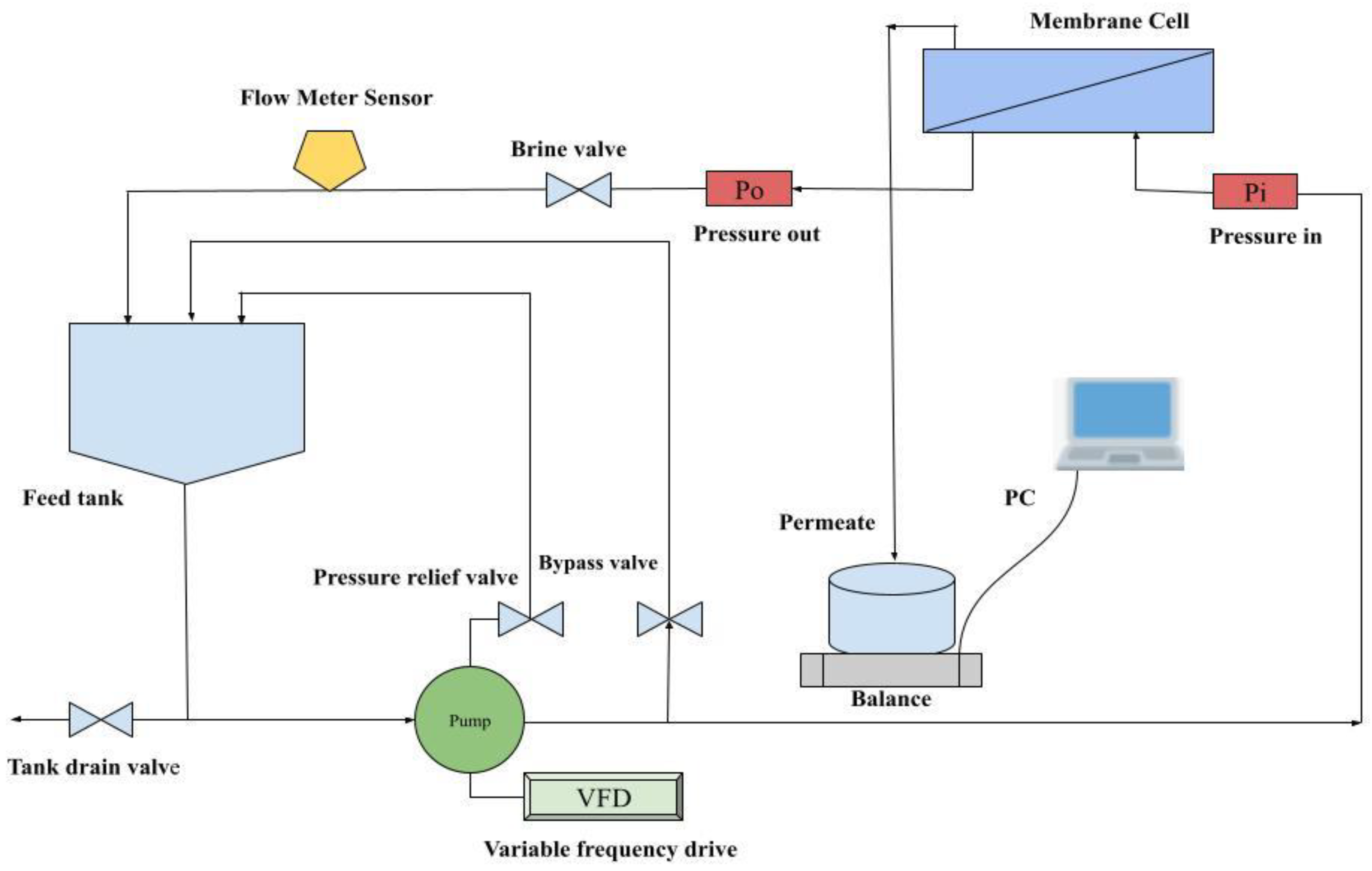
Figure 2.
Rejection rates of MgSO4 in different runs.
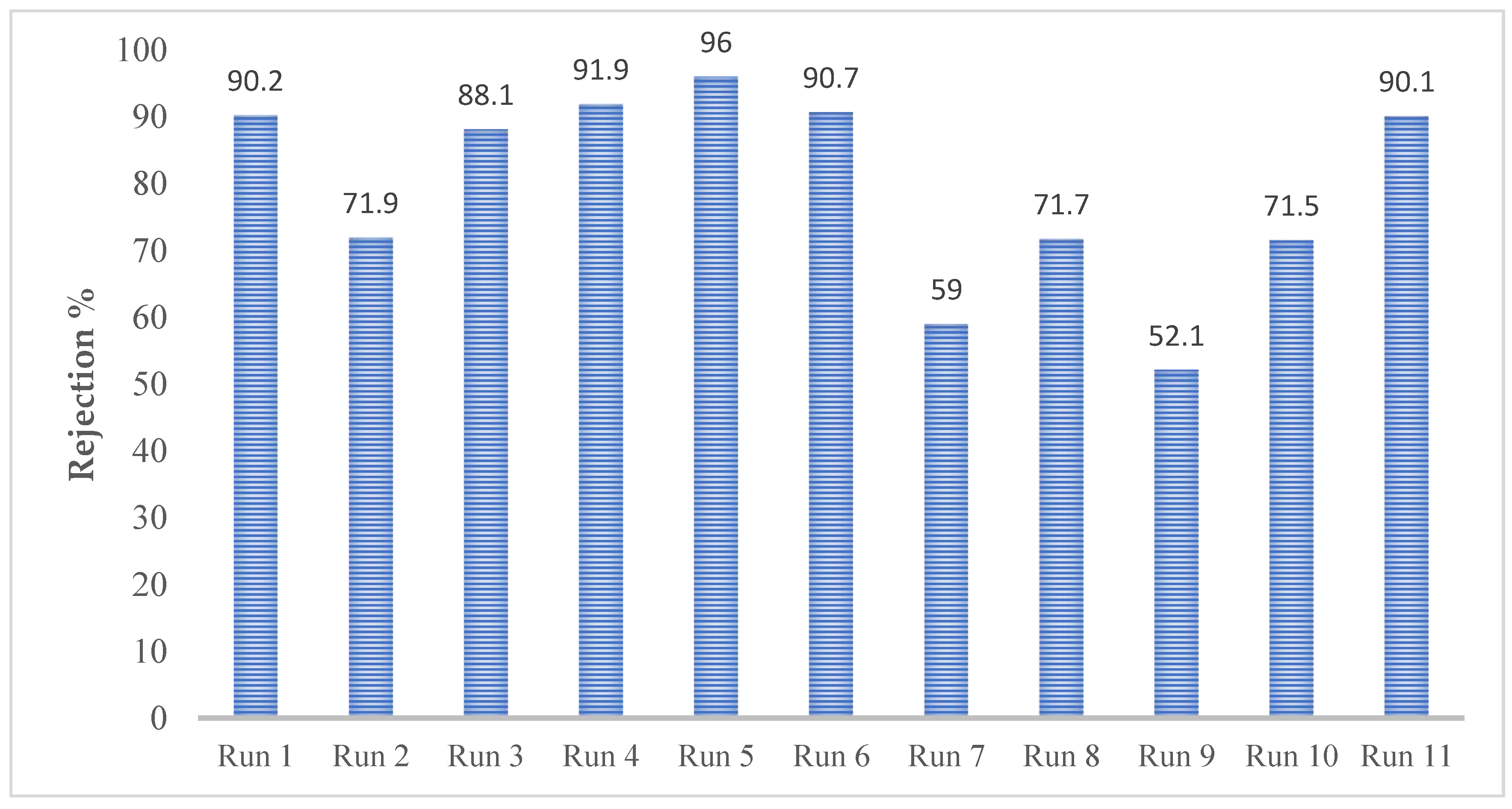
Figure 3.
Decline in permeate flux as a function of time for the eleven runs.
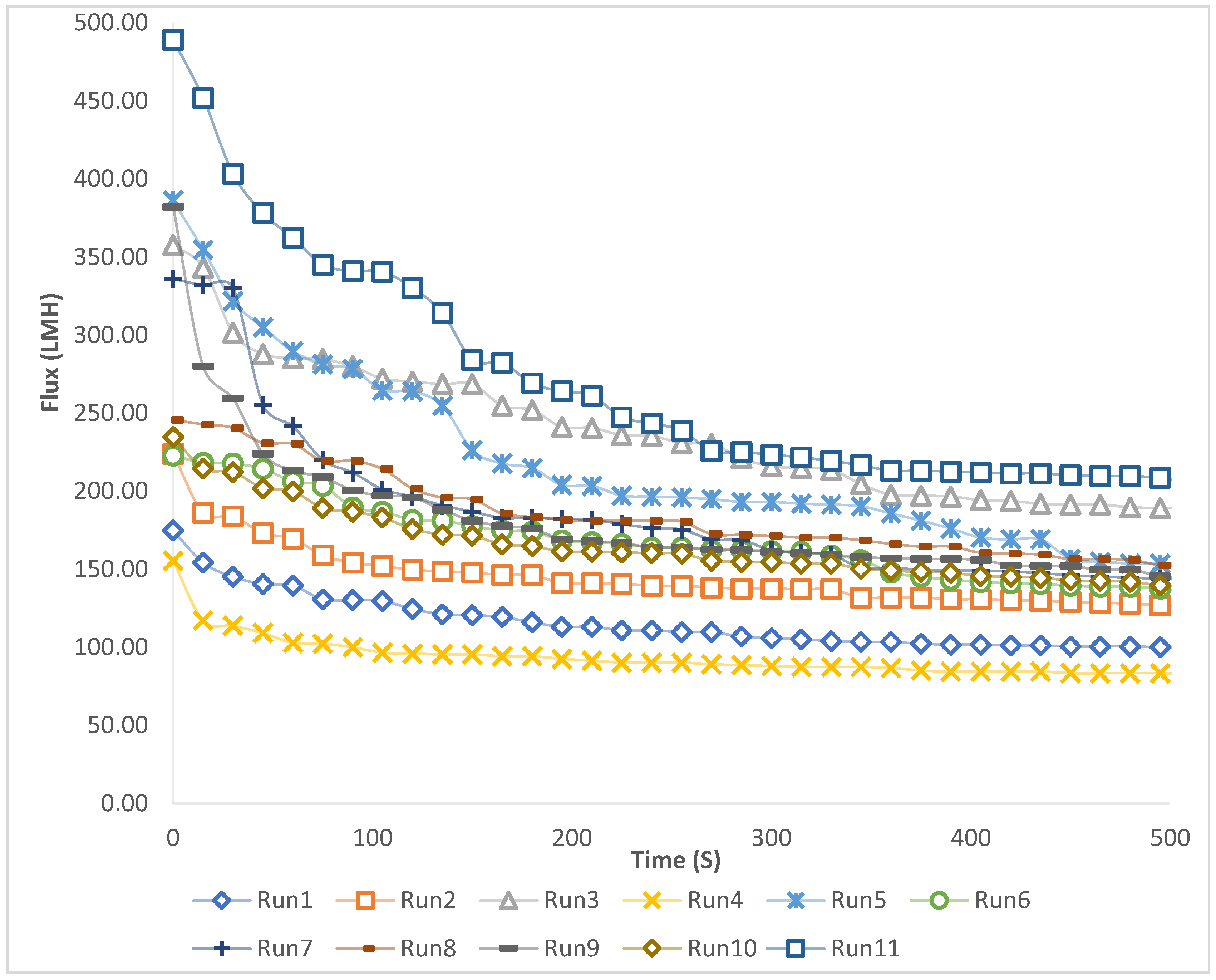
Figure 4.
(A,B) Standardized effects of variables on membrane rejection rate and permeate flux.
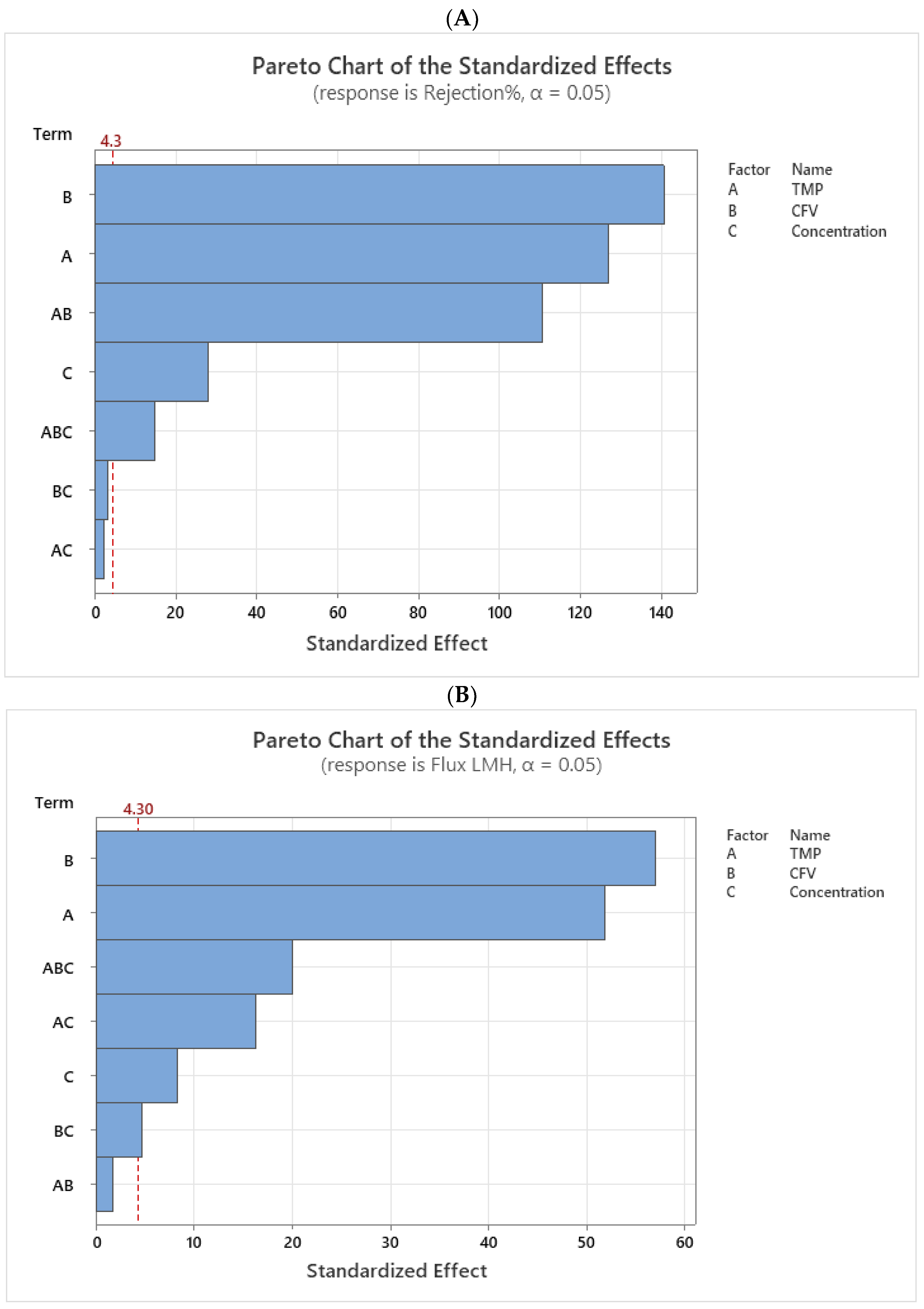
Figure 5.
(A). Illustration of the interaction plot for the rejection rate. (B). Illustration of the interaction plot for the flux.
Figure 5.
(A). Illustration of the interaction plot for the rejection rate. (B). Illustration of the interaction plot for the flux.
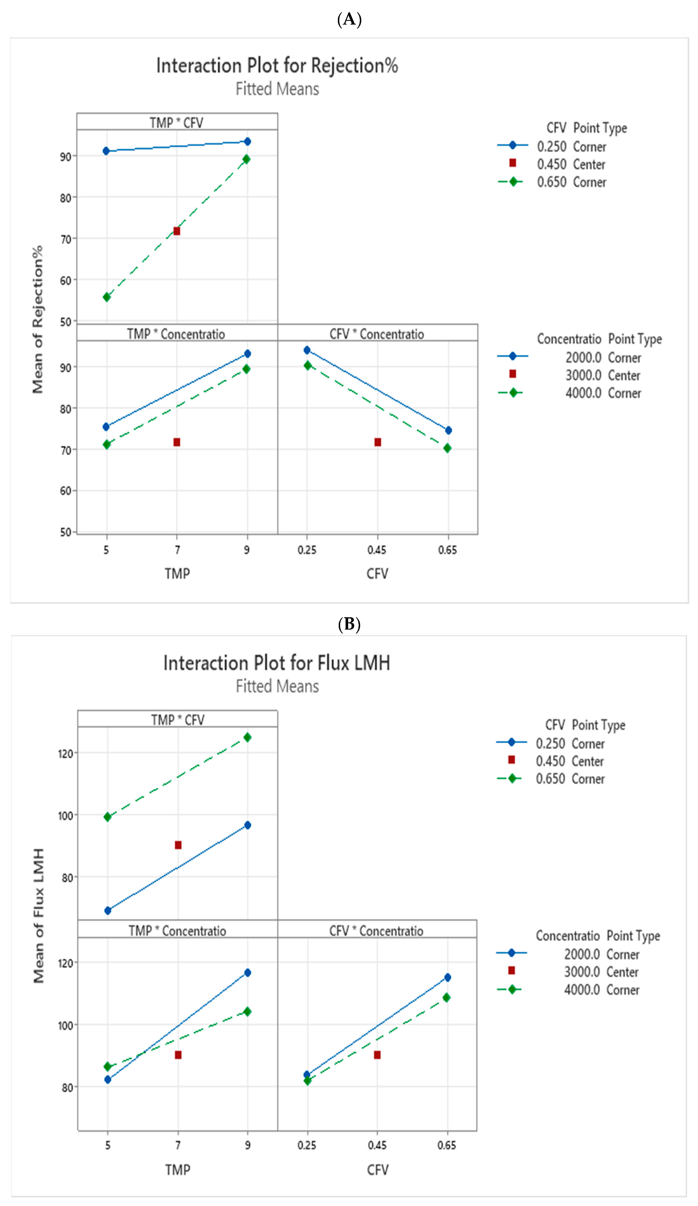
Figure 6.
Cube for: (A) Rejection in % and (B) Flux in LMH.
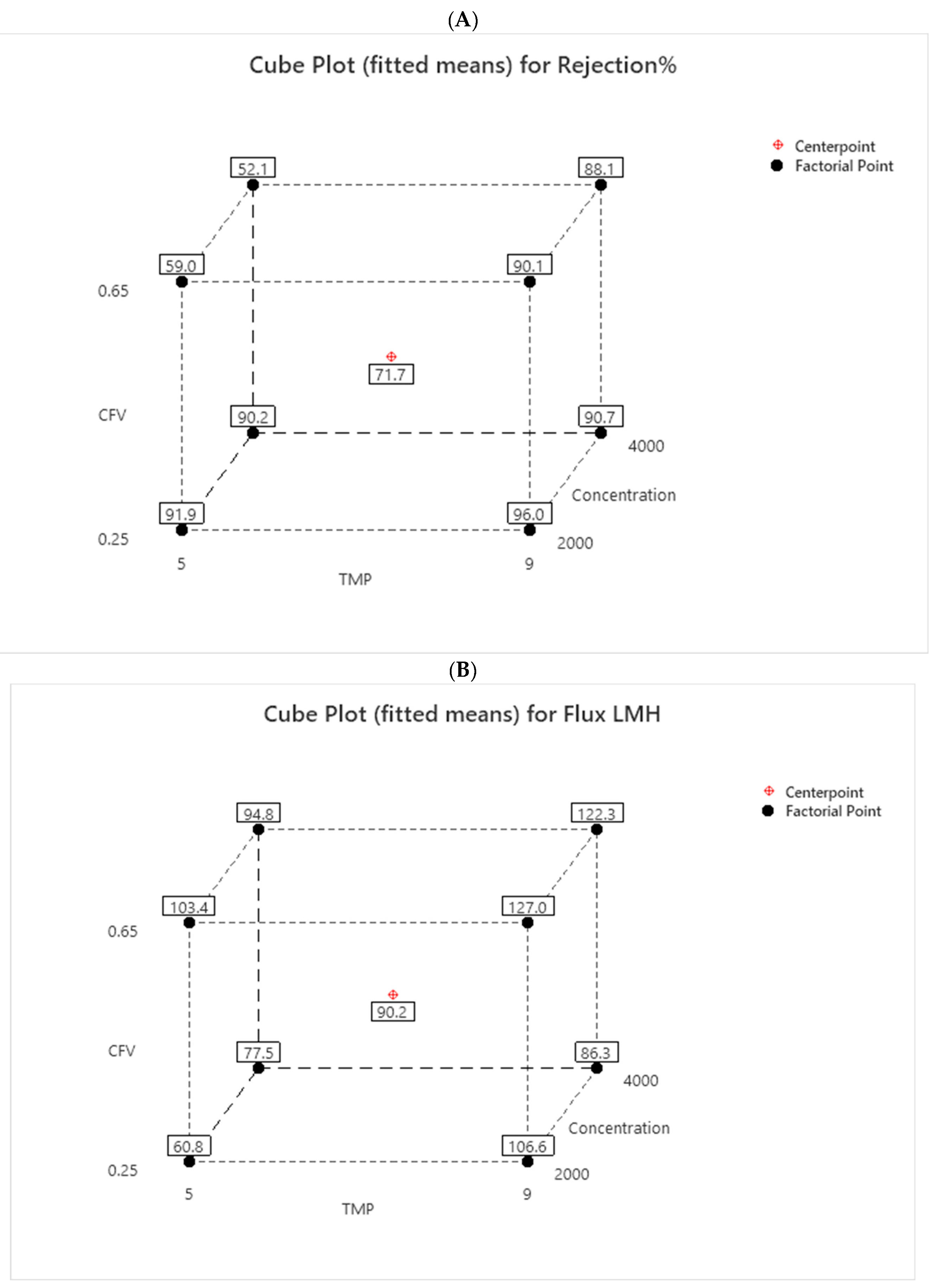
Figure 7.
The response optimizer model generates optimization plots (parameters and composite desirability values).
Figure 7.
The response optimizer model generates optimization plots (parameters and composite desirability values).
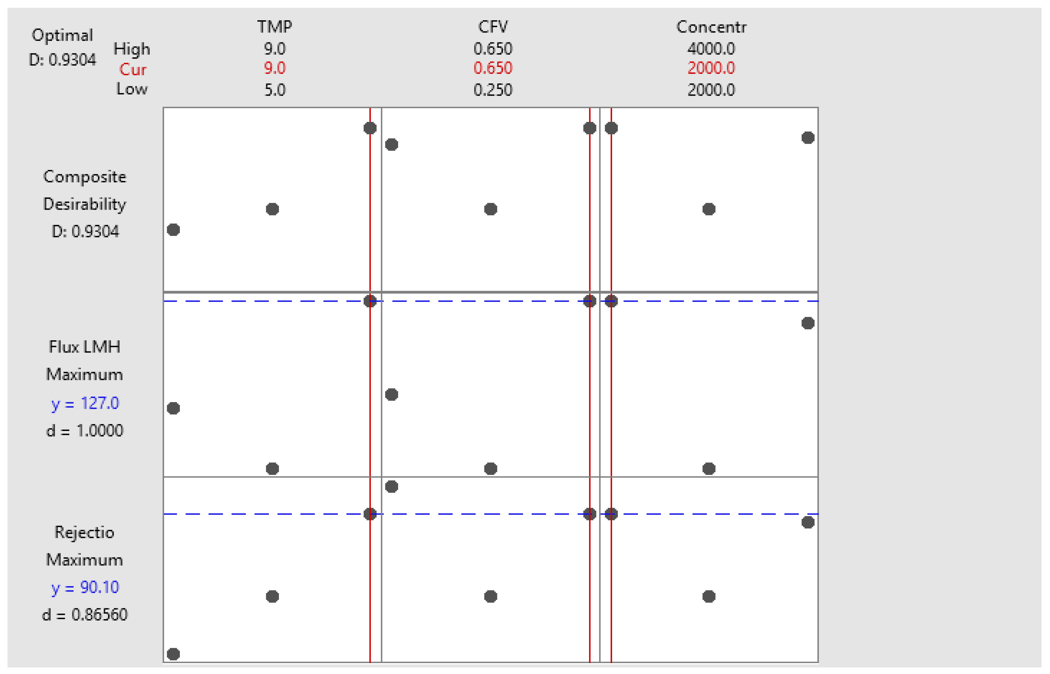
Figure 8.
Perfect prediction vs. actual permeate flux correlation response for (A) DT and (B) RF.
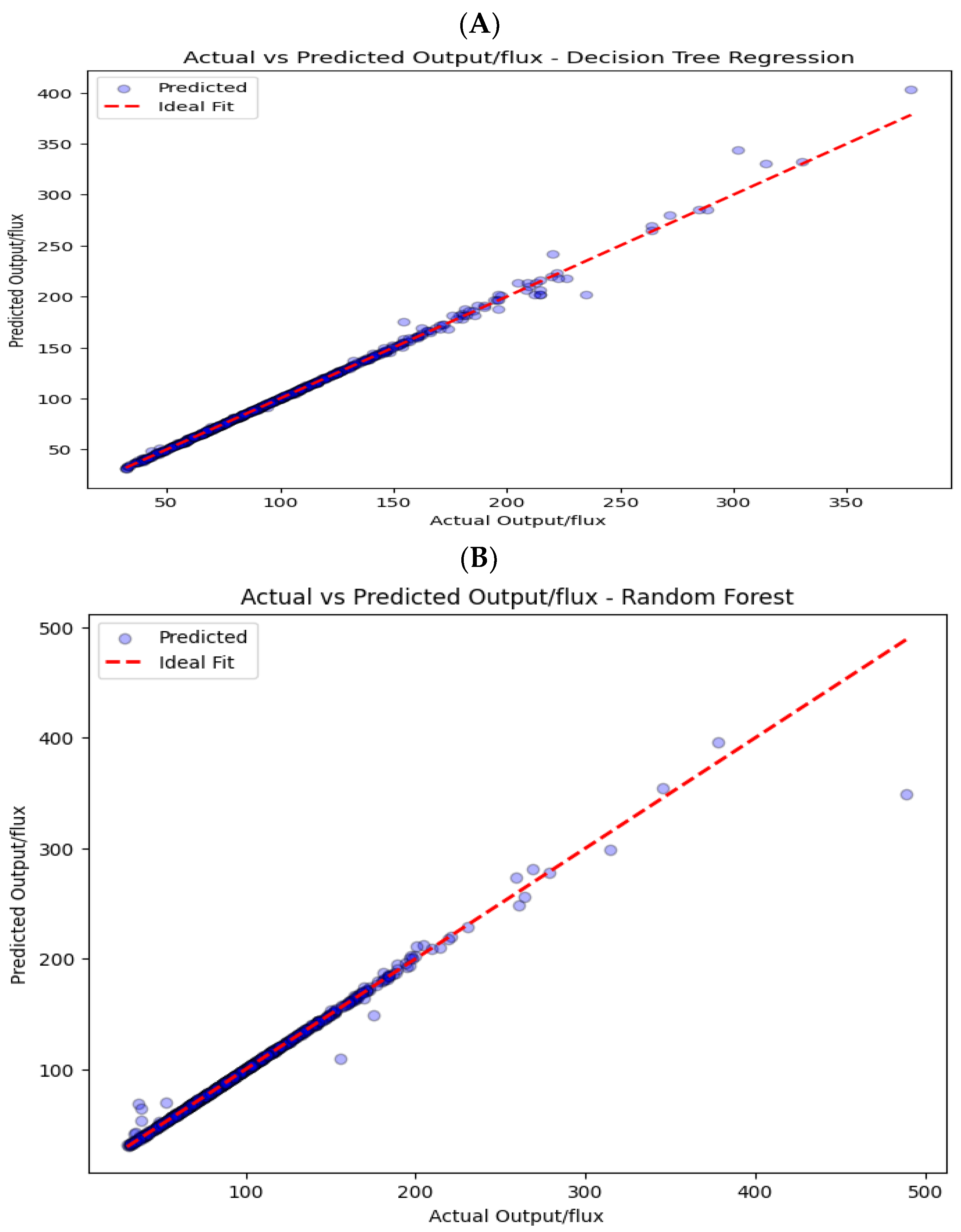
Figure 9.
Illustration of actual versus predicted flux values for: (A) DT model and (B) RF model.
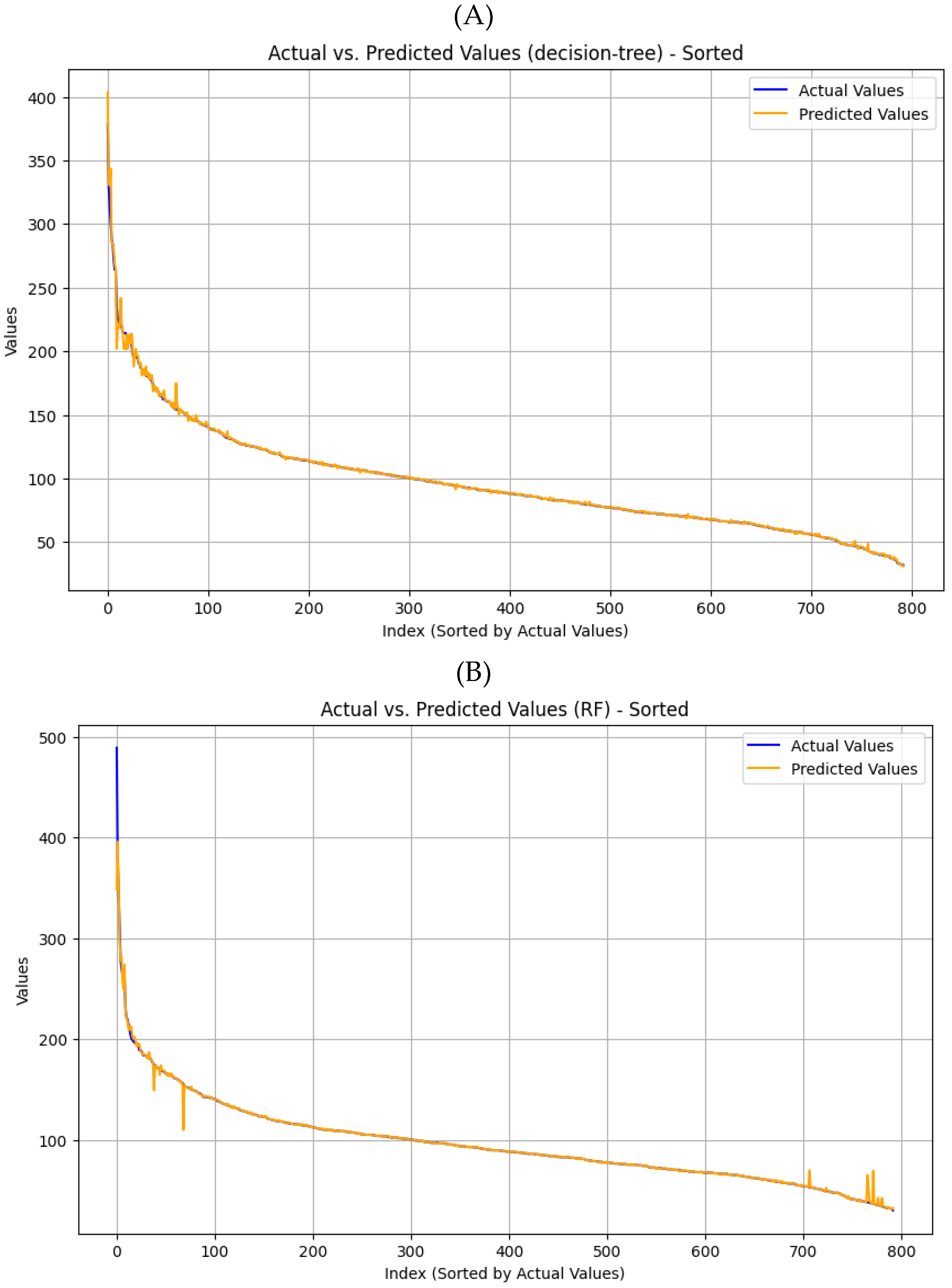

Table 1.
List of parameters used with units and standard deviations (SD).
| Parameter | Unit | SD |
|---|---|---|
| TMP | bar | ±0.2 |
| CFV | m/s | ±0.02 |
| EC | µS/cm | ±25 |
| MgSO4 | mg/L | ±20 |
| pH | - | ±0.2 |
Table 2.
Membrane features and characterization.
| Brand of membrane | NF90 |
|---|---|
| Manufacturing | Dow-FilmTec, USA |
| Weight Cut-Off (MWCO) | 200-400 |
| Polymer materials | TFC- polyamide |
| pH range (25 oC) | 2-11 |
| Temperature max | 40 oC |
| Module | Flat sheet |
Table 3.
Independent variables and their levels.
| Variables | Code design | Low (- 1) | Middle (0) | High (+1) |
|---|---|---|---|---|
| TMP (bar) | A | 5 | 7 | 9 |
| CFV (m/s) | B | 0.25 | 0.45 | 0.65 |
| MgSO4 concentration (mg/L) | C | 2,000 | 3,000 | 4,000 |
Table 4.
Coded variables and their corresponding levels.
| Std Order | Run Order | TMP (bar) | CFV (m/s) | Concentration (mg/L) |
|---|---|---|---|---|
| 5 | 1 | -1 | -1 | +1 |
| 10 | 2 | 0 | 0 | 0 |
| 8 | 3 | +1 | +1 | +1 |
| 1 | 4 | -1 | -1 | -1 |
| 2 | 5 | +1 | -1 | -1 |
| 6 | 6 | +1 | -1 | +1 |
| 3 | 7 | -1 | +1 | -1 |
| 11 | 8 | 0 | 0 | 0 |
| 7 | 9 | -1 | +1 | +1 |
| 9 | 10 | 0 | 0 | 0 |
| 4 | 11 | +1 | +1 | -1 |
Table 5.
Full factorial design variables and their experimental results for rejection and flux.
| Std Order | Run Order | TMP (bar) | CFV (m/s) | Concentration (mg/L) | Rejection (%) | Flux (LMH) |
| 5 | 1 | 5 | 0.25 | 4,067 | 90.2 | 77.5 |
| 10 | 2 | 7 | 0.45 | 3,054 | 71.9 | 89.6 |
| 8 | 3 | 9 | 0.65 | 4,046 | 88.1 | 122.3 |
| 1 | 4 | 5 | 0.25 | 2,048 | 91.9 | 60.8 |
| 2 | 5 | 9 | 0.25 | 2,035 | 96.0 | 106.6 |
| 6 | 6 | 9 | 0.25 | 4,057 | 90.7 | 86.3 |
| 3 | 7 | 5 | 0.65 | 2,055 | 59.0 | 103.4 |
| 11 | 8 | 7 | 0.45 | 3,071 | 71.7 | 91.0 |
| 7 | 9 | 5 | 0.65 | 4,062 | 52.1 | 94.8 |
| 9 | 10 | 7 | 0.45 | 3,076 | 71.5 | 90.0 |
| 4 | 11 | 9 | 0.65 | 2,052 | 90.1 | 127 |
Table 6.
Rejection rates for all experimental runs.
| Run # | Conductivity µS/cm | Rejection% | |
|---|---|---|---|
| Feed (µS/cm) | Permeate (µS/cm) | ||
| Run 1 | 4221 | 413 | 90.2 |
| Run 2 | 3367 | 946 | 71.9 |
| Run 3 | 4201 | 498 | 88.1 |
| Run 4 | 2400 | 193 | 91.9 |
| Run 5 | 2398 | 95 | 96.0 |
| Run 6 | 4210 | 389 | 90.7 |
| Run 7 | 2408 | 985 | 59.0 |
| Run 8 | 3372 | 953 | 71.7 |
| Run 9 | 4218 | 2017 | 52.1 |
| Run 10 | 3378 | 962 | 71.5 |
| Run 11 | 2403 | 236 | 90.1 |
Table 7.
ANOVA for rejection rate.
| Source | DF | SS | MS | F-Value | P-Value |
|---|---|---|---|---|---|
| Model | 8 | 2205.64 | 275.70 | 6893 | 0.000 |
| Linear | 3 | 1464.24 | 488.08 | 12202 | 0.000 |
| TMP | 1 | 642.61 | 642.61 | 16065 | 0.000 |
| CFV | 1 | 790.03 | 790.03 | 19751 | 0.000 |
| Concentration | 1 | 31.60 | 31.60 | 790 | 0.001 |
| 2-Way Interactions | 3 | 488.94 | 162.98 | 4074 | 0.000 |
| TMP*CFV | 1 | 488.28 | 488.28 | 12207 | 0.000 |
| TMP*Concentration | 1 | 0.21 | 0.211 | 5.28 | 0.148* |
| CFV*Concentration | 1 | 0.45 | 0.451 | 11.28 | 0.078* |
| 3-Way Interactions | 1 | 9.03 | 9.03 | 225.78 | 0.004 |
| TMP*CFV*Concentration | 1 | 9.03 | 9.03 | 225.78 | 0.004 |
| Curvature | 1 | 243.42 | 243.42 | 6085 | 0.000 |
| Error | 2 | 0.08 | 0.040 | ||
| Total | 10 | 2206 |
* Not statistically significant at a 95% confidence level.
Table 8.
ANOVA for permeate flux.
| Source | DF | SS | MS | F-Value | P-Value |
|---|---|---|---|---|---|
| Model | 8 | 3593 | 449.18 | 863.81 | 0.001 |
| Linear | 3 | 3123 | 1041 | 2002 | 0.000 |
| TMP | 1 | 1396 | 1396 | 2686 | 0.000 |
| CFV | 1 | 1691 | 1691 | 3251 | 0.000 |
| Concentration | 1 | 35.70 | 35.70 | 68.66 | 0.014 |
| 2-Way- Interactions | 3 | 150.24 | 50.08 | 96.31 | 0.010 |
| TMP*CFV | 1 | 1.53 | 1.53 | 2.94 | 0.228* |
| TMP*Concentration | 1 | 136.95 | 136.95 | 263.37 | 0.004 |
| CFV*Concentration | 1 | 11.76 | 11.76 | 22.62 | 0.041 |
| 3-Way- Interactions | 1 | 209.10 | 209.10 | 402.12 | 0.002 |
| TMP*CFV*Concentration | 1 | 209.10 | 209.10 | 402.12 | 0.002 |
| Curvature | 1 | 111.15 | 111.15 | 213.75 | 0.005 |
| Error | 2 | 1.04 | 0.52 | ||
| Total | 10 | 3594 |
* Not statistically significant at a 95% confidence level.
Table 9.
Influence of variables on the predicted response.
| Response | Goal | Lower | Target | Upper | Weight | Importance |
|---|---|---|---|---|---|---|
| Flux LMH | Maximum | 60.8 | 127 | 127 | 1 | 2 |
| Rejection% | Maximum | 52.1 | 96 | 96 | 1 | 2 |
Table 10.
Composite desirability by operating conditions.
| Solution | TMP | CFV | Concentration | Flux (LMH) Fit |
Rejection (%) Fit |
Composite Desirability |
|---|---|---|---|---|---|---|
| 1 | 9 | 0.65 | 2000 | 127.0 | 90.1 | 0.93 |
| 2 | 9 | 0.65 | 4000 | 122.3 | 88.1 | 0.87 |
Disclaimer/Publisher’s Note: The statements, opinions and data contained in all publications are solely those of the individual author(s) and contributor(s) and not of MDPI and/or the editor(s). MDPI and/or the editor(s) disclaim responsibility for any injury to people or property resulting from any ideas, methods, instructions or products referred to in the content. |
© 2025 by the authors. Licensee MDPI, Basel, Switzerland. This article is an open access article distributed under the terms and conditions of the Creative Commons Attribution (CC BY) license (http://creativecommons.org/licenses/by/4.0/).
Copyright: This open access article is published under a Creative Commons CC BY 4.0 license, which permit the free download, distribution, and reuse, provided that the author and preprint are cited in any reuse.


