
Submitted:
30 June 2025
Posted:
30 June 2025
You are already at the latest version
Abstract
Anomalous and normal diffusion processes are characterized by the time evolution of the mean square displacement of a diffusing molecule σ2(t). When σ2(t) is a power function of time, the process is described by fractional subdiffusion, fractional superdiffusion or normal diffusion equation. However, for other forms of σ2(t), the diffusion equations are often not defined. We show that to describe diffusion characterized by σ2(t), the g-subdiffusion equation with the fractional Caputo derivative with respect to a function g can be used. Choosing an appropriate function g we obtain the Green’s function for this equation, which generates the assumed σ2(t). A method for solving such an equation, based on the Laplace transform with respect to the function g, is also described.
Keywords:
g–subdiffusion
; fractional caputo derivative with respect to another function
; anomalous diffusion
; fractional calculus
1. Introduction
Anomalous diffusion models are often based on the assumption of constant parameters, which means that the structure of the medium remains constant over time. A frequently used model to derive the normal and anomalous diffusion equations is the continuous time random walk (CTRW) model [1,2,3,4,5]. Within this model, random walk of a single molecule is considered. The process is described by the probability density (Green’s function) of finding the molecule at point x at time t, being the initial position of the molecule. In a one-dimensional unbounded homogeneous system (such a system is considered in this paper) the mean square displacement (MSD) of a molecule is calculated as
The relation
is often used to define the type of diffusion. For we have subdiffusion, then
is the subdiffusion coefficient measured in the units of . Subdiffusion occurs in a system in which the movement of diffusing molecules is very hindered, as occurs in gels, porous media, and bacterial biofilms [2,6,7,8,9,10]. For we have normal diffusion with . When we have superdiffusion (facilitated diffusion), the examples are diffusion in turbulent media and in random velocity fields [11,12,13,14], cell migration in some biological processes [15], movement of endogeneous intracellular particles in some pathogens [16], and mussels movement [17]. However, the CTRW model gives . The superdiffusion model, based on the g-subdiffusion equation, which provides is shown in Refs. [18,19]. The relation (2) is complemented by the following relation defining ultraslow diffusion (slow subdiffusion)
where v is a slowly varying function that satisfies the condition when for any . In practice, v is a combination of logarithmic functions. Ultraslow diffusion is an extremely slow process, qualitatively different from ordinary subdiffusion. This process has been observed in diffusion of water in aqueous sucrose glasses [20] and languages dynamics [21]. Superdiffusion is usually described by an equation with a fractional derivative with respect to the spatial variable, while subdiffusion is described by an equation with a fractional derivative with respect to time. Ultraslow diffusion is described by integro–differential equations with integral operators which are not usually identified as fractional time derivatives [22,23,24,25,26,27,28].
Differential equations mentioned above with constant parameters are used to describe diffusion in a medium which properties does not change with time. However, diffusion parameters depend on the interaction of diffusing molecules with the environment and on a structure of the medium, both can change over time. The single molecule tracking method allows for the experimental determination of . We mention that there have been used other power functions with respect to time, experimentally measurable, from which subdiffusion parameters can be determined. An example of this is the time evolution of the so-called thickness of the membrane layer [8]. Processes with a time-varying diffusion exponent have been observed in bacterial motion on small beads in a freely suspended soap film [29], in transport of colloidal particles between two parallel plates [30], microspheres in a living eukaryotic cell [31], endogenous lipid granules in living yeast cells [32], and in the diffusion of passive molecules in the active bath with moving particles [33,34]. According to the Stokes-Einstein formula, , the change of the temperature T of a liquid generates the change in the diffusion coefficient. It was found that the diffusion coefficient of chloride ions in concrete shows a dependence on time [35,36]. Other examples are which is caused by the aging process of a complex system in which anomalous diffusion occurs [37] and , where a and b are constant parameters [38]. Experimental study provided that the diffusion model with power-law well describes water diffusion in brain tissues [39,40]. The function can have a more complicated form, e.g. it may contain an oscillatory component. Such a dependency can occur, for example, in diffusion of antibiotics in bacterial biofilms. Bacteria activate various defense mechanisms against the action of antibiotics [41,42]. One such mechanism is the thickening of the biofilm, which significantly impedes diffusion of the antibiotic and reduces the diffusion coefficient. Slowing down diffusion of the antibiotic reduces the risk of the antibiotic having an effective effect on the bacteria. This process can cause a relaxation of the defense mechanisms of bacteria and increase diffusion of the antibiotic. Bacteria, feeling a greater threat, intensify their defense mechanisms again, and so on. The subdiffusion coefficient of the antibiotic in the biofilm may then undergo periodic changes. Diffusion coefficients that oscillate with time, reflecting complex memory or frictional effects in the system, have been considered in some fractional diffusion models [43].
When the diffusion parameters are not constant, various equations have been used to describe the diffusion processes such as subdiffusion equations with a fractional time derivative of the order depending on time (and on a spatial variable) [44,45,46,47,48,49,50,51,52,53,54,55], and the equation with a linear combination of fractional time derivatives of different orders [56].
If the function has a complicated form, the question arises as to what equation describes the subdiffusion process and whether there are methods for solving such an equation. We will show that by using the g-subdiffusion equation with an appropriately chosen function g one can describe the diffusion process defined by a time-increasing function . The Green’s function for this equation generates the assumed function . The g-subdiffusion equation contains the Caputo derivative with respect to the function g [57,58]. This equation can be solved using the Laplace transform with respect to the function g (the g-Laplace transform).
2. G-Subdiffusion Equation
The CTRW model provides the following ordinary subdiffusion equation
where , the Caputo fractional derivative is defined for as
. Formally, the normal diffusion equation
can be treated as a special case of the subdiffusion equation for . We mention that Eq. (5) can be transformed to its equivalent form with the fractional Riemann–Liouville time derivative of the order [2,3,4,7],
The g–subdiffusion equation can be interpreted as a modified form of Eq. (5). The modification consists of changing the time variable t to a function , , where is given in units of time and meets the conditions , , and . The g–subdiffusion equation is [57,58]
where the g-Caputo fractional derivative of the order with respect to the function g is defined for as [59]
When , the g-Caputo fractional derivative takes the form of the ordinary Caputo derivative. The Green’s function is a solution to a subdiffusion equation for the initial conditions , where is the delta–Dirac function. In an unbounded region the boundary conditions are assumed to be .
The g–subdiffusion equation can be solved by means of the g–Laplace transform method. The g-Laplace transform is defined as [60,61]
The g–Laplace transform is related to the ordinary Laplace transform ,
Eq. (11) provides the relation
The above formula is helpful in calculating the inverse g–Laplace transform if the inverse ordinary Laplace transform is known. For example, since , , and , , we get [62,63]
and
. The function is a special case of the Wright function and the H-Fox function.
The calculations for solving Eq. (8) by means of the g–Laplace transform method are similar to those for solving Eq. (5) using the ordinary Laplace transform. Due to the relation [60,61]
where , the g–Laplace transform of Eq. (8) reads
The g–Laplace transform of Green’s function, that is the following solution to Eq. (16) for the boundary conditions , is
3. Time Evolution of as a Function Defining the Diffusion Process
As mentioned in Sec. Section 1, the function is usually used as a definition of the type of diffusion. The function is experimentally measurable. The single particle tracking method is used when a random walk of a single molecule is observed [64,65,66,67]. The function can also be determined in another way, e.g. by studying the release of a substance from one vessel to another through a thin membrane. At the initial moment, the vessel A contains a homogeneous solution of the diffusing substance with an initial concentration , the subdiffusion parameters in the vessel are and , and the vessel B contains a pure solvent. When the membrane allows free passage from the vessel A to B, and the molecule return passage is practically impossible, then the total amount of the substance N in the vessel B evolves in time as , where [68]. Combining these equations with Eqs. (2) and (3) we get . Another method is to measure the temporal evolution of the thickness of near-membrane layer . It is defined as the distance from the membrane to the point, where the substance concentration drops k times with respect to the membrane surface in the vessel B. We get , where is controlled by , , and k, see [8].
In the case where evolves in time according to Eq. (2), the equations describing the diffusion process are known. However, as mentioned in Sec. Section 1, more complicated forms of are possible for which the equation describing the process may not be known. Based on our considerations in Sec. Section 2, we conclude that such a process can be described by the g-subdiffusion equation Eq. (8), in which
see Eq. (19). The Green’s function is given by Eq. (18). When the molecules diffuse independently of each other, the concentration C of the diffusing molecules can be calculated using the formula
Then, the g-subdiffusion equation is also satisfied by the function .
As an example, we consider four cases of the function , two of which contain an oscillating component.
- Forwe have
- Whenwe get
- Whenthere is
- Forwe get
In the above equations it is assumed that , , and .
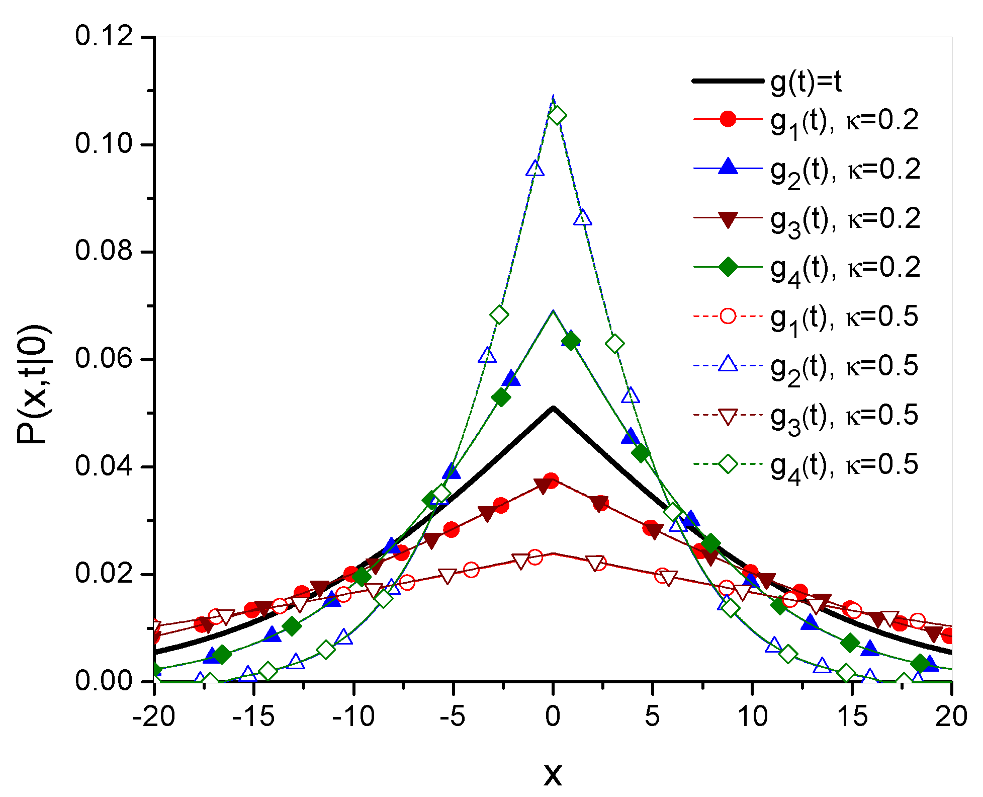
The time evolutions of the mean square displacement of diffusing particle are given in Figs. Figure 1 and Figure 2. Figs. Figure 3 and Figure 4 show the Green’s function plots for times and , respectively. The plots of the functions are compared with the functions obtained for ordinary subdiffusion with constant parameters and , for which and , that are marked with a thick solid line without symbols. All plots are made for the function , , defined by Eqs. (23), (25), (27), and (29), respectively; the numbering of other functions is consistent with the numbering of the function . The plots are made for , , , , , and , the values of all parameters are given in arbitrarily chosen units. In each case two values of , namely and , are considered. Comparing and with and , respectively, in Fig. Figure 2 we see how the oscillatory effect changes . The effect, involved in the functions and , is visible for relatively short times. This fact can also be seen by analyzing the plots of Green’s functions. In Fig. Figure 3, for , the plots of the functions generated by and differ from each other, and the same applies to the functions generated by and . These differences almost disappear in Fig. Figure 4 for .
4. Final Remarks
We have used the g-subdiffusion equation to describe diffusion process defined by the function . This equation contains the time fractional Caputo derivative with respect to an increasing function . As , the g-subdiffusion equation becomes the ordinary subdiffusion equation. The function given by Eq. (20) provides an equation describing the process characterized by a time-increasing function that can be determined experimentally. The presented model confirms the usefulness of the g-subdiffusion equation in modeling anomalous diffusion processes.
The function is criticized as not defining the type of diffusion unambiguously. As shown in Ref. [69], the appropriate combination of superdiffusion and subdiffusion effects provides the relation , but such a process cannot be interpreted as normal diffusion. However, is an important characteristic of the diffusion process. In our considerations, we use this function as defining the diffusion process, without defining the type of diffusion based on Eq. (2).
For diffusion processes defined by Eq. (2), the diffusion equations are derived from the stochastic CTRW model. The g-subdiffusion equation also has its stochastic interpretation [58]. It can be derived from the modified CTRW model. The interpretation of this equation is based on the assumption that the time variable t is replaced by a time-increasing function with the additional assumptions and . If the function has the same properties, then, together with the parameters and , the function defines . Then, the process can be described by the g-subdiffusion equation. The parameters and are determined from additional considerations. For example, the drug transport in a system containing densely packed gel beads is described by the g-subdiffusion equation, which is confirmed by empirical studies [68]. However, in the initial time interval, this process is well described by the ordinary subdiffusion equation Eq. (5), for which the parameters can be determined.
Author Contributions
Conceptualization and methodology, T.K., A.D.; formal analysis, T.K., A.D., K.L.; writing—original draft preparation, T.K., A.D.; writing—review and editing, T.K., A.D., K.L. All authors have read and agreed to the published version of the manuscript.
Funding
This research received no external funding.
Institutional Review Board Statement
Not applicable.
Data Availability Statement
The original contributions presented in this study are included in the article. Further inquiries can be directed to the corresponding author.
Conflicts of Interest
The authors declare no conflicts of interest.
References
- Montroll, E.W.; Weiss, G.H. Random walks on lattices II. J. Math. Phys. 1965, 167. [Google Scholar] [CrossRef]
- Metzler, R.; Klafter, J. The random walk’s guide to anomalous diffusion: a fractional dynamics approach. Phys. Rep. 2000, 339, 1–77. [Google Scholar] [CrossRef]
- Compte, A. Stochastic foundations of fractional dynamics. Phys. Rev. E 1996, 53, 4191–4193. [Google Scholar] [CrossRef] [PubMed]
- Klafter, J.; Sokolov, I.M. First step in random walks. From tools to applications. Oxford UP, New York, 2011. [CrossRef]
- Barkai, E.; Metzler, R.; Klafter, J. From continuous time random walks to the fractional Fokker-Planck equation. Phys. Rev. E 2000, 61, 132–138. [Google Scholar] [CrossRef]
- Bouchaud, J.P.; Georgies, A. Anomalous diffusion in disordered media: statistical mechanisms, models and physical applications. Phys. Rep. 1990, 195, 127–293. [Google Scholar] [CrossRef]
- Metzler, R.; Klafter, J. The restaurant at the end of the random walk: recent developments in the description of anomalous transport by fractional dynamics. J. Phys. A 2004, 37, R161–R208. [Google Scholar] [CrossRef]
- Kosztołowicz, T.; Dworecki, K.; Mrówczyński, S. How to measure subdiffusion parameters. Phys. Rev. Lett. 2005, 94, 170602. [Google Scholar] [CrossRef]
- Kosztołowicz, T.; Metzler, R. Diffusion of antibiotics through a biofilm in the presence of diffusion and absorption barriers. Phys. Rev. E bf 2020, 102, 032408. [Google Scholar] [CrossRef]
- Kosztołowicz, T.; Metzler, R.; Wa̧sik, S.; Arabski, M. Modelling experimentally measured of ciprofloxacin antibiotic diffusion in Pseudomonas aeruginosa biofilm formed in artificial sputum medium. PLoS One 2020, 15(12), e0243003. [Google Scholar] [CrossRef]
- Redner, S. Superdiffusive transport due to random velocity fields. Physica D: Nonlin. Phenom. 1989, 38, 287. [Google Scholar] [CrossRef]
- Zumofen, G.; Klafter, J.; Blumen, A. Enhanced diffusion in random velocity fields. Phys. Rev. A 1990, 42, 4601. [Google Scholar] [CrossRef] [PubMed]
- Bouchaud,J. P.; Georges, A.; Koplik, J.; Provata, A.; Redner, S. Superdiffusion in random velocity fields. Phys. Rev. Lett. 1990, 64, 2503. [Google Scholar] [CrossRef] [PubMed]
- Compte, A.; Cáceres, M. O. Fractional dynamics in random velocity fields. Phys. Rev. Lett. 1998, 81, 3140. [Google Scholar] [CrossRef]
- Dieterich, P.; Klages, R.; Preuss, R.; Schwab, A. Anomalous dynamics of cell migration. Proc. Natl. Acad. Sci. USA 2008, 105, 459. [Google Scholar] [CrossRef]
- Reverey, J. F.; Jeon, J. H.; Bao, H.; Leippe, M.; Metzler, R.; Selhuber–Unkel, C. Superdiffusion dominates intracellular particle motion in the supercrowded cytoplasm of pathogenic Acanthamoeba castellanii. Sci. Rep. 2015, 5, 11690. [Google Scholar] [CrossRef]
- de Jager, M.; Weissing, F. J.; Herman, P. M. J.; Nolet, B. A.; van de Koppel, J. Lévy walks evolve through interaction between movement and environmental complexity. Science 2011, 332, 1551. [Google Scholar] [CrossRef]
- Kosztołowicz, T. Subdiffusion equation with fractional Caputo time derivative with respect to another function in modeling transition from ordinary subdiffusion to superdiffusion. Phys. Rev. E 2023, 107, 064103. [Google Scholar] [CrossRef]
- Kosztołowicz, T. Subdiffusion Equation with Fractional Caputo Time Derivative with Respect to Another Function in Modeling Superdiffusion. Entropy 2025, 27, 48. [Google Scholar] [CrossRef]
- Zorbist, B.; Soonsin, V.; Luo, B.P.; Krieger, U.K.; Marcolli, C.; Peter, T.; Koop, T. Ultra-slow water diffusion in aqueous sucrose glasses. Phys. Chem. Chem. Phys. 2011, 13, 3514. [Google Scholar]
- Watanabe, H. Empirical observations of ultraslow diffusion driven by the fractional dynamics in languages, Phys. Rev. E 2018, 98, 012308. [Google Scholar]
- Chechkin, A.V.; Klafter, J.; Sokolov, I.M. Fractional Fokker-Planck equation for ultraslow kinetics. Europhys. Lett. 2003, 63, 326. [Google Scholar] [CrossRef]
- Chechkin, A.V.; Kantz, H.; Metzler, R. Ageing effects in ultraslow continuous time random walks. Eur. Phys. J. B 2017, 90, 205. [Google Scholar] [CrossRef]
- Denisov, S.I.; Kantz, H. Continuous-time random walk with a superheavy-tailed distribution of waiting times. Phys. Rev. E 2011, 83, 041132. [Google Scholar] [CrossRef] [PubMed]
- Denisov, S.I.; Yuste, S.B.; Bystrik, Yu.S.; Kantz, H.; Lindenberg, K. Asymptotic solutions of decoupled continuous-time random walks with superheavy-tailed waiting time and heavy-tailed jump length distributions. Phys. Rev. E 2011, 84, 061143. [Google Scholar] [CrossRef]
- Kosztołowicz, T. Subdiffusive random walk in a membrane system. J. Stat. Mech. P 2015, 10021. [Google Scholar] [CrossRef]
- Sanders, L.P.; Lomholt, M.A.; Lizana, L.; Fogelmark, K.; Metzler, R.; Abjörnsson, T. Severe slowing-down and universality of the dynamics in disordered interacting many-body systems: ageing and ultraslow diffusion. New J. Phys. 2014, 16, 113050. [Google Scholar] [CrossRef]
- Bodrova, A.S.; Chechkin, A.V.; Cherstvy, A.G. and Metzler, R. Ultraslow scaled Brownian motion. New J. Phys. 2015, 17, 063038. [Google Scholar] [CrossRef]
- Wu, X. L.; Libchaber, A. Particle diffusion in a quasi-two-dimensional bacterial bath. Phys. Rev. Lett. 2000, 84, 3017. [Google Scholar] [CrossRef]
- Chakrabarty, A.; Konya, A.; Wang, F.; Selinger, J. V.; Sun, K.; Wei, Q. H. Brownian motion of boomerang colloidal particles. Phys. Rev. Lett. 2013, 111, 160603. [Google Scholar] [CrossRef]
- Caspi, A.; Granek, R.; Elbaum, M. Enhanced diffusion in active intracellular transport. Phys. Rev. Lett. 2002, 85, 011916. [Google Scholar] [CrossRef]
- Jeon, J. H.; Tejedor, V.; Burov, S.; Barkai, E.; Selhuber-Unkel, C.; Berg-Sørensen, K.; Oddershede, L.; Metzler, R. In vivo anomalous diffusion and Weak ergodicity breaking of lipid granules. Phys. Rev. Lett. 2011, 106, 048103. [Google Scholar] [CrossRef] [PubMed]
- Miño, G.; Mallouk, T. E.; Darnige, T.; Hoyos, M.; Dauchet, J.; Dunstan, J.; Soto, R.; Wang, Y.; Rousselet, A.; Clement, E. Enhanced diffusion due to active swimmers at a solid surface. Phys. Rev. Lett. 2011, 106, 048102. [Google Scholar] [CrossRef] [PubMed]
- Bechinger, C.; Di Leonardo, R.; Löwen, H.; Reichhard, C.; Volpe, G.; Volpe, G. Active particles in complex and crowded environments. Rev. Mod. Phys. 2016, 88, 045006. [Google Scholar] [CrossRef]
- Ma, J.; Yang, Q.; Wang, X.; Peng, X.; Qin, F. Review of Prediction Models for Chloride Ion Concentration in Concrete Structures. Buildings 2025, 15, 149. [Google Scholar] [CrossRef]
- Luping, T; Nilsson, L. O. Chloride diffusivity in high strength concrete at different ages. Nord. Concr. Res. 1992, 11, 162–171. [Google Scholar]
- Lomholt, M. A.; Lizana, L.; Metzler, R.; Ambjornsson, T. Microscopic origin of the logarithmic time evolution of aging processes in complex systems. Phys. Rev. Lett. 2013, 110, 208301. [Google Scholar] [CrossRef]
- Cherstvy, A. G.; Safdari, H.; Metzler, R. Anomalous diffusion, nonergodicity, and ageing for exponentially and logarithmically time-dependent diffusivity: striking differences for massive versus massless particles. J. Phys. D: Appl. Phys. 2021, 54, 195401. [Google Scholar] [CrossRef]
- Novikov, D. S.; Fieremans, E.; Jespersen, S. N.; Kiselev, V. G. Quantifying brain microstructure with diffusion MRI: theory and parameter estimation NMR. Biomed, 3998; 32. [Google Scholar]
- Lee, H-H. ; Papaioannou, A.; Kim, S-L.; Novikov D. S.; Fieremans, E. Probing axonal swelling with time dependent diffusion MRI Commun. Biol. 2020, 3, 354.
- Anderson, G.G.; O’Toole, G.A. Bacterial Biofilms. Current Topics in Microbiology and Immunology 2008, 322, p–85. [Google Scholar] [CrossRef]
- Mah, T.F.C.; O’Toole, G.A. Mechanisms of biofilm resistance to antimicrobial agents. Trends Microbiol. 2001, 9, 34–39. [Google Scholar] [CrossRef]
- Bao, J. D. Time-Dependent Fractional Diffusion and Friction Functions for Anomalous Diffusion. Front. Phys. 5671; :61. [Google Scholar] [CrossRef]
- Sun, H. G.; Chen, W.; Chen, Y. Variable-order fractional differential operators in anomalous diffusion modeling. Physica A 2009, 388, 4586. [Google Scholar] [CrossRef]
- Sun, H. G.; Chen, W.; Sheng, H.; Chen, Y. On mean square displacement behaviors of anomalous diffusions with variable and random orders. Phys. Lett. A 2010, 374, 906. [Google Scholar] [CrossRef]
- Sun, H. G.; Chen, W.; Li, C.; Chen, Y. Finite difference schemes for variable-order time fractional diffusion equation. Int. J. Bifurcat. Chaos 2012, 22, 1250085. [Google Scholar] [CrossRef]
- Chen, W.; Zhang, J.; Zhang, J. A variable-order time-fractional derivative model for chloride ions sub-diffusion in concrete structure. Fract. Calc. Appl. Analys. 2013, 16, 76–92. [Google Scholar] [CrossRef]
- Sun, H. G.; Chang, A.; Zhang, Y.; Chen, W. A review on variable-order fractional differential equations: Mathematical foundations, physical models, and its applications. Frac. Calc. Appl. Anal. 2019, 22, 27. [Google Scholar] [CrossRef]
- Yang, Z.; Zheng, X.; Wang, H. A variably distributed-order time-fractional diffusion equation: Analysis and approximation. Comput. Methods Appl. Mech. Engrg. 2020, 367, 113118. [Google Scholar] [CrossRef]
- Liang, Y.; Wang, S.; Chen, W.; Zhou, Z.; Magin, R. L. A survey of models of ultraslow diffusion in heterogeneous materials. Appl. Mech. Rev. 2019, 71, 040802. [Google Scholar] [CrossRef]
- Roth, P.; Sokolov, I. M. Inhomogeneous parametric scaling and variable-order fractional diffusion equations. Phys Rev. E 2020, 102, 012133. [Google Scholar] [CrossRef]
- Awad, E.; Sandev, T.; Metzler, R.; Chechkin, A. Closed-form multi-dimensional solutions and asymptotic behaviors for subdiffusive processes with crossovers: I. Retarding case. Chaos Solit. Fract. 2021, 152, 111357. [Google Scholar] [CrossRef]
- Awad, E.; Metzler, R. Crossover dynamics from superdiffusion to subdiffusion: Models and solutions. Frac. Calc. Appl. Anal. 2020, 23, 55. [Google Scholar] [CrossRef]
- Patnaik, S.; Hollkamp, S.; Semperlotti, J. P. Applications of variable-order fractional operators: a review. Proc. R. Soc. A 2020, 476, 20190498. [Google Scholar] [CrossRef] [PubMed]
- Fedotov, S.; Han, D. Asymptotic behavior of the solution of the space dependent variable order fractional diffusion equation: ultraslow anomalous aggregation. Phys. Rev. Lett. 2009, 123, 050602. [Google Scholar] [CrossRef] [PubMed]
- Bazhlekova, E. Completely monotone multinomial Mittag–Leffler type functions and diffusion equations with multiple time-derivative. Frac. Calc. Appl. Analys. 2021, 24, 88. [Google Scholar] [CrossRef]
- Kosztołowicz, T.; Dutkiewicz, A. Subdiffusion equation with Caputo fractional derivative with respect to another function. Phys. Rev. E 2021, 104, 014118. [Google Scholar] [CrossRef]
- Kosztołowicz, T.; Dutkiewicz, A. Stochastic interpretation of g-subdiffusion process. Phys. Rev. E 2021, 104, L042101. [Google Scholar] [CrossRef]
- Almeida, R. A Caputo fractional derivative of a function with respect to another function. Commun. Nonlinear Sci. Numer. Simulat. 2017, 44, 460–481. [Google Scholar] [CrossRef]
- Jarad, F.; Abdeljawad, T. Generalized fractional derivatives and Laplace transform. Discrete And Continuous Dynamical Systems Series S 2020, 13, 709–722. [Google Scholar] [CrossRef]
- Jarad, F.; Abdeljawad, T.; Rashid, S.; Hammouch, Z. More properties of the proportional fractional integrals and derivatives of a function with respect to another function. Adv. Differ. Equ. 2020, 303. [Google Scholar] [CrossRef]
- Kosztołowicz, T. From the solutions of diffusion equation to the solutions of subdiffusive one. J. Phys. A: Math. Gen. 2004, 37, 10779–10789. [Google Scholar] [CrossRef]
- Fahad, H.M.; Rehman, M.; Fernandez, A. On Laplace transforms with respect to functions and their applications to fractional differential equations. Math Meth. Appl Sci. 2021, 1–20. [Google Scholar] [CrossRef]
- Weiss, M. Resampling single-particle tracking data eliminates localization errors and reveals proper diffusion anomalies. Phys. Rev. E 2019, 100, 042125. [Google Scholar] [CrossRef] [PubMed]
- Michalet, X.; Berglund A., J. Optimal diffusion coefficient estimation in single-particle tracking. Phys. Rev. E 2012, 85, 061916. [Google Scholar] [CrossRef] [PubMed]
- Kepten, E.; Bronshtein, I.; Garini, Y. Improved estimation of anomalous diffusion exponents in single-particle tracking experiments. Phys. Rev. E 2013, 87, 052713. [Google Scholar] [CrossRef] [PubMed]
- Bailey, M. L. P.; Yan, H.; Surovtsev, I.; Williams J., F.; King M., C.; Mochrie S. G., J. Covariance distributions in single particle tracking. Phys. Rev. E 2021, 103, 032405. [Google Scholar] [CrossRef]
- Kosztołowicz, T.; Dutkiewicz, A.; Lewandowska, K. D.; Wa̧sik, S.; Arabski, M. Subdiffusion equation with Caputo fractional derivative with respect to another function in modelling diffusion in a complex system consisting of matrix and channels. Phys. Rev. E 2022, 106, 044138. [Google Scholar] [CrossRef]
- Dybiec, B.; Gudowska–Nowak, E. Discriminating between normal and anomalous random walks. Phys. Rev. E 2009, 80, 061122. [Google Scholar] [CrossRef]
Figure 1.
Time evolution of the MSD for the cases described in the legend.
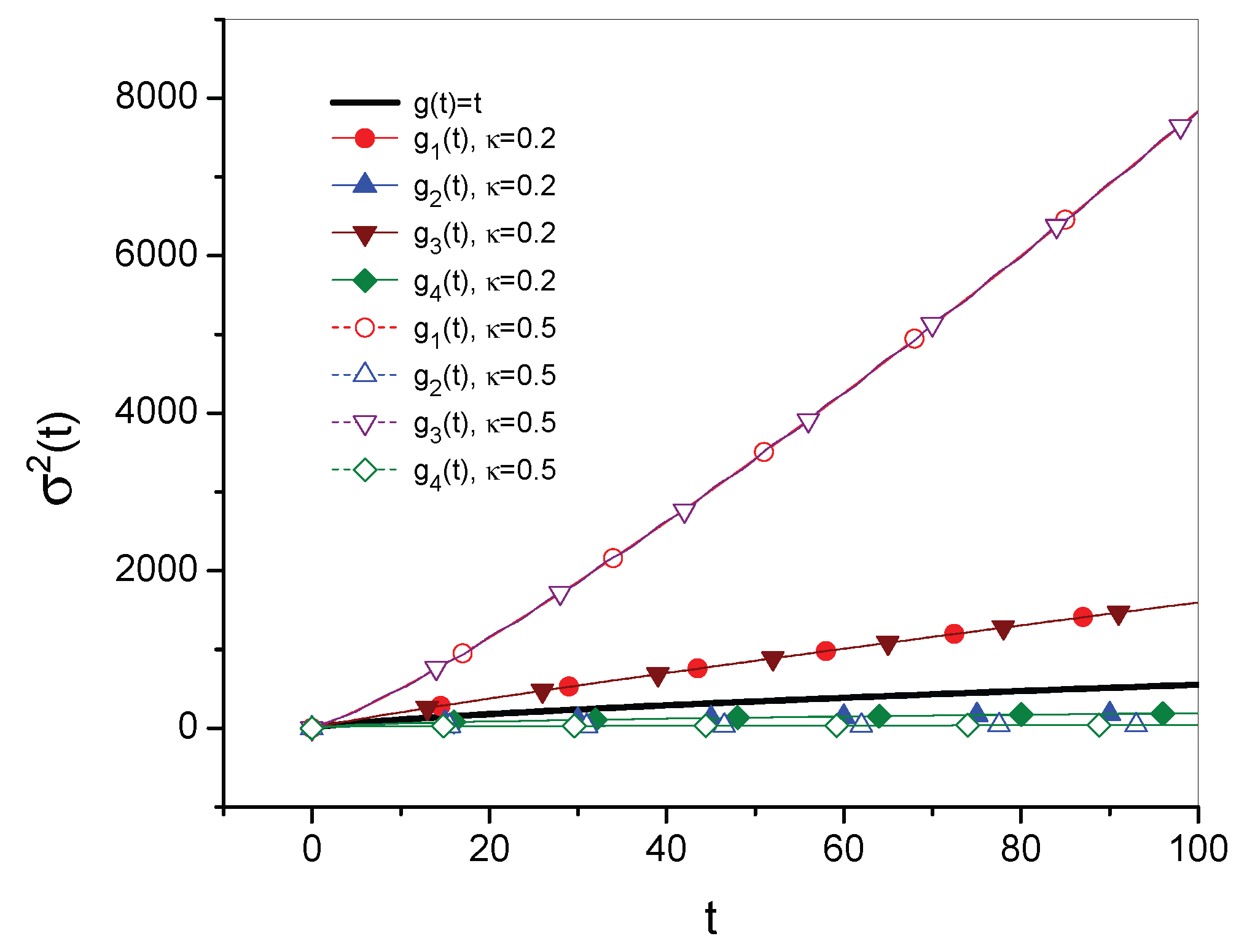
Figure 2.
Fragment of Fig. Figure 1 for relatively short times. The differences in the functions generated by and , as well as by and , are caused by the oscillation term in and ; the legend, omitted in this Figure, is the same as in Fig. Figure 1.
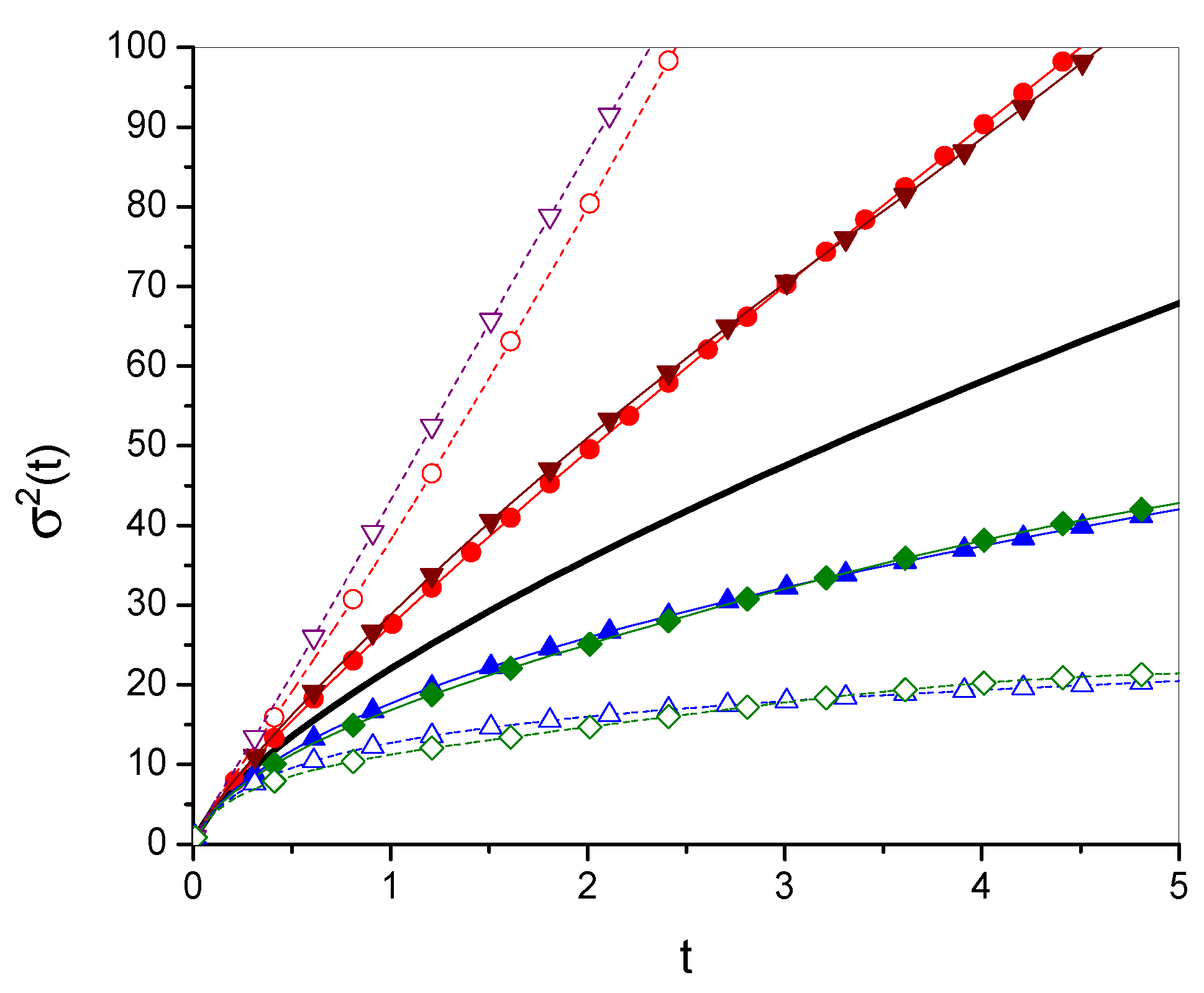
Figure 3.
Plots of Green’s functions for , additional description is in the text.
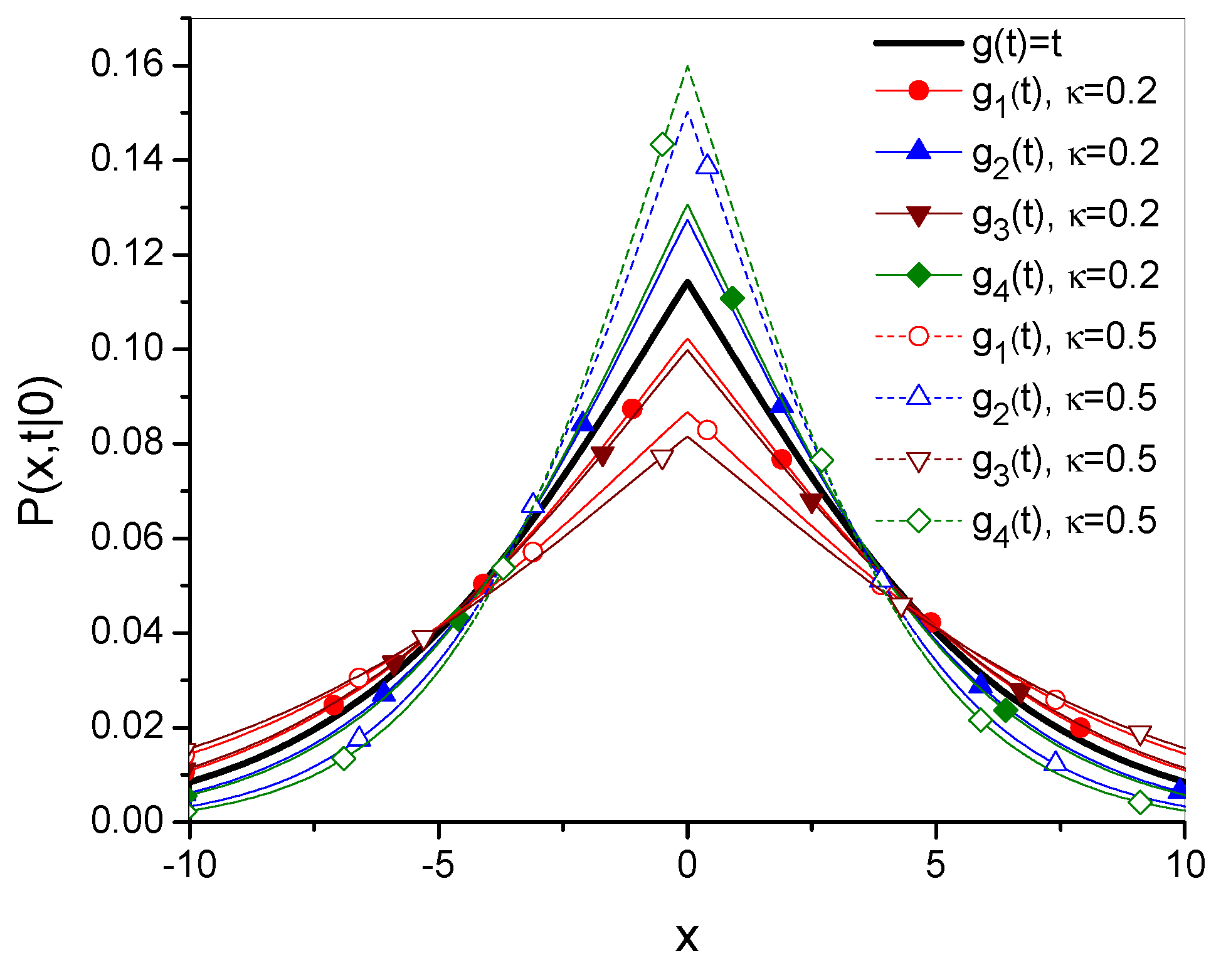
Figure 4.
Plots of Green’s functions for .
Disclaimer/Publisher’s Note: The statements, opinions and data contained in all publications are solely those of the individual author(s) and contributor(s) and not of MDPI and/or the editor(s). MDPI and/or the editor(s) disclaim responsibility for any injury to people or property resulting from any ideas, methods, instructions or products referred to in the content. |
© 2025 by the authors. Licensee MDPI, Basel, Switzerland. This article is an open access article distributed under the terms and conditions of the Creative Commons Attribution (CC BY) license (http://creativecommons.org/licenses/by/4.0/).
Copyright: This open access article is published under a Creative Commons CC BY 4.0 license, which permit the free download, distribution, and reuse, provided that the author and preprint are cited in any reuse.


