Submitted:
30 June 2025
Posted:
30 June 2025
You are already at the latest version
Abstract
The article analyzes the operating principle of the BMM sensor emitter in order to improve the accuracy of wireless determination of the BMM sensor coordinates under a massif of destroyed rock in the context of problems of determining the shift of rocks during gold ore mining. Using numerical simulation, FEM has been developed to develop digital models reflecting individual cases of the propagation of the magnetic field of the emitter located in various geological conditions and positions relative to the rock surface and the vertical axis. The accuracy of determining the coordinates of the radio beacon in the rock has been analyzed, data on the deviation of the coordinates of the peaks of the magnetic field strength from the radio beacon axis have been obtained in cases of a heterogeneous composition of the rock massif, the influence of the deviation of the emitter axis angle from the vertical, the influence of the unevenness of the collapse relief and the influence of the superposition of fields from different radiation sources. A study has been carried out to determine the direction of the radio beacon search based on the resulting vector of the emitter's magnetic field strength.
Keywords:
magnetic dipole
; rock displacement sensor
; coordinate search
; broken-rock disintegration
; modeling
; low-resistance clusters
; coordinate determination error
1. Introduction
Blasting operations are a critical aspect of the mineral extraction cycle that facilitates rock fragmentation for easier ore excavation. However, they simultaneously exert significant and measurable impacts on ore grade control and variability (grade control). This occurs due to complex rock movement affecting post-blast processes [1,2]. Previous research on blast optimization [3,4,5] demonstrated that visual delineation between ore and waste becomes entirely indistinct after blasting, making grade control exceptionally challenging. While fragmentation remains the primary objective, blast-induced movement must be accounted for to improve post-blast ore boundary definition, thereby reducing ore loss and dilution [1,6,7,8].
Quality control of valuable component extraction remains one of the most critical tasks in open-pit metal mining under conditions of heterogeneous mineral distribution in ore bodies. This task becomes particularly relevant when mining native gold, where ore grades can vary by orders of magnitude over distances of mere meters. Statistical methods with block models based on exploration drilling data are used to delineate boundaries between ore zones of different metal grades and waste material [9]. These models track the displacement of marked ore masses after drilling and blasting operations. The identified boundaries between ore and waste rock shift following bench blasting, rendering them inaccurate for guiding ore excavation lines. This rock displacement caused by blasting operations adversely affects ore-waste separation, leading to either misclassification of ore components into waste streams, resulting in valuable material losses, or incorrect delineation of ore quality boundaries, causing ore dilution. Such ore loss and dilution impose significant economic impacts on mining operations, as they directly reduce recovery rates during subsequent processing stages.
For direct measurement of rock displacement caused by blasting in open-pit mines, various methods are implemented with varying success. These methods primarily rely on measuring rock displacement at several discrete locations within the blast area. The methods are divided into two types based on the devices used for measurement [2,10]:
- visual markers (sandbags, colored chains, colored pipes);
- remote sensing sensors.
The measuring devices are installed in surveyed locations within the rock mass prior to blasting, in special boreholes without explosives, and their new positions are determined after blasting. The vector between pre- and post-blast positions of each sensor can be used to analyze the magnitude and direction of displacement at specific points caused by blasting. The primary drawback of visual markers is that the measuring devices may be lost beneath the crushed rock pile. For this reason, rock displacement results after blasting remain unavailable until the rock material is excavated, rendering the data obsolete.
Unlike visual markers, remote sensing methods employ trackable sensors emitting electromagnetic signals. Such systems include transmitters in polymer casings placed in individual boreholes before blasting, with their coordinates localized after blasting using electromagnetic detectors. After obtaining the new sensor coordinates, the data is processed to determine displacement vectors of specific points caused by blasting [11].
Detection of these sensors beneath the ore mass within the rock pile is performed along N-S and W-E oriented profiles. Registration occurs by detecting sensor fields at the surface using a magnetic antenna oriented strictly horizontally. Precise determination of new sensor coordinates is a critical task.
The article subsequently examines various factors introducing errors in coordinate determination for displacement sensors located within rock piles at depths up to 6 m. An assessment of coordinate determination errors will be performed using a digital model of the rock pile after blasting.
2. Materials and Methods
Determining changes in the coordinates of a rock displacement sensor involves locating its position in three-dimensional space beneath a layer of collapsed rock at depths up to 6 m. This allows establishing the degree of sensor displacement in space and approximating rock movement to define collapse boundaries. BMM sensors are identified using a low-frequency magnetic field at 30–80 kHz. The most suitable frequency for sensor detection is 66 kHz [12]. A low-frequency electromagnetic signal is preferred because the influence of electrophysical properties on it is significantly less than on high-frequency signals.
The sensor signal is generated via a magnetic coil housed within a plastic casing [12,13,14]. The design of some rock displacement sensors includes a mechanism for orienting the transmitting antenna (coil) vertically. This effect is achieved by shifting the center of mass below the device’s central point. To reduce resistance between the device and the inner spherical housing, a gap filled with fluid (water or oil) is provided. Thus, the solenoid always orients vertically, which is critical for minimizing coordinate identification errors.
The sensor’s magnetic fields are generated by a magnetic coil (Figure 1) wound around a plastic housing containing a power cell and control board. This assembly is enclosed within a sphere or other-shaped casing immersed in a liquid medium, all housed within the sensor’s external spherical shell [15].
The magnetic field strength of the coil is determined by the equation [16]:
where I is the current flowing through the coil;
w is the number of turns;
l is the coil length.
The magnetic induction parameter is determined by the equation:
where μ0 = 4·π·10–7 H/m is the magnetic constant;
μr is the relative magnetic permeability of the medium where the coil is located.
For a vertically oriented magnetic coil without a ferrite core, the induction at distance r is determined as [16]:
where r is the distance from the coil to the measurement point; S is the area of the coil turn; θ is the angle between the normal n of the solenoid and the observation point P (in polar coordinates).
For detection, a receiving antenna (transponder) in the form of a magnetic loop is used, which registers the vertical magnetic field of a solenoid located inside the sensor. The general principle of distance measurement using magnetic transponders is presented through the analysis of the ratio of induction or signals from the radial and axial components of the magnetic field H or magnetic induction B, respectively. The accuracy of the method is achieved due to the fact that the attenuation dependencies of the magnetic induction vector B in space are inversely proportional to the cube of the distance and weakly depend on the absorbing properties of the rocks. In the polar coordinate system, the magnetic induction B value at a distance from the dipole can be written as [17]:
Bφ = 0,
where M=w·I·S is the antenna magnetic moment.
The cubic dependence of the amplitude decay of the magnetic induction vector on distance results in limited operational range of transmitters (radio beacons) and necessitates a wide dynamic range of signal amplitudes at the input of the transponder’s receiving path.
Figure 2a shows the magnetic induction lines in the near field. The magnetic induction vector B represents the vector sum of the radial (Bᵣ) and axial (Bθ) components. Under quasi-stationary magnetic field conditions, all sources can be considered point-like. The coordinate determination scheme for the measurement point and the magnetic induction field lines of a dipole in the digital sensor model embedded in rock formations are shown in Figure 2(b). The most stable magnetic field distribution is observed directly above the dipole, which is also utilized when searching for BMM sensors with vertical antenna orientation mechanisms [14,18].
The search for BMM sensors in a collapsed rock mass is performed by recording the axial component of the magnetic field. The method is based on zoning the surface of the rock collapse with a detector equipped with a loop receiving antenna. Probing is conducted along North-South and West-East oriented lines [18]. The coordinates of displaced sensors after rock collapse are determined by the maximum of the axial component of the magnetic field. Modeling will allow evaluating two key parameters of the sensor search method under a rock mass:
– accuracy of coordinate determination on both flat surfaces and in models of heterogeneous rock debris piles;
– feasibility of an alternative method for detecting sensor fields without probing the search area via a grid, using directional indications from the recorded axial and radial components.
Rock Analysis
When an electromagnetic field propagates through a continuous medium characterized by physical properties of dielectric permittivity, magnetic permeability, and electrical conductivity, these parameters influence both the attenuation rate of its field strength with distance and the wavelength. The attenuation of the electromagnetic field in a continuous medium can be evaluated through the attenuation coefficient and wave number [19]:
Thus, the instantaneous strength of the magnetic component of the wave incident on the air-rock interface varies according to the law:
where is the instantaneous magnetic field strength of the electromagnetic field; is the instantaneous magnetic field strength at the air/rock interface boundary; z is the depth of wave penetration into the solid medium.
Physical properties of the medium also affect the wavelength of the electromagnetic field passing through it:
From this, it can be deduced that when propagating through rocks, the wavelength of the electromagnetic field decreases with increasing values of the rocks’ electrophysical properties.
BMM sensors are most actively used in gold deposit development, where distinguishing gold content in ore is a critical parameter for improving the efficiency of mined raw material beneficiation. According to electrical exploration data from the Digo-Digo gold deposit (central Brazil), the specific electrical resistance of rocks with varying gold content ranges from 20 to 7200 Ω·m, corresponding to specific electrical conductivity of 0.05 to 1.38·10⁻⁴ S/m [20].
Gold-bearing ores are characterized by significant diversity in material and chemical composition [21]. The most common mineral in ores is quartz, with content ranging from 10% to 90%. Additionally, ores contain iron sulfides (pyrite, marcasite), copper sulfide (chalcopyrite), as well as arsenic sulfides (arsenopyrite), lead sulfides (galena), and zinc sulfides (sphalerite). Ores contain various quantities of other non-sulfide minerals—oxides, carbonates, tourmalines, and magnetite. The host rocks for gold-bearing ores are granites, schists, and others.
If gold ore contains other non-ferrous metals in industrial concentrations, such ore is called gold-polymetallic, and its processing technology must include both gold extraction and production of enriched non-ferrous metal concentrates. Based on sulfide mineral content, gold-bearing ores are classified as low-sulfide (3-4% sulfides), medium-sulfide (4-10% sulfides), sulfide (10-30% sulfides). The most frequently encountered are quartz-sulfide-gold ore deposits, which hold the greatest industrial significance. Sulfide ores typically occur as deposits, veins, and disseminated grains. In these ores, gold exists as finely dispersed and dust-like particles. Gold is extracted as a byproduct alongside copper, zinc, and pyrite concentrates. It should be noted that simple quartz ores—easily processed with straightforward gold extraction—have become extremely rare worldwide. Often, sulfides in ores exist in oxidized or semi-oxidized forms, leading to ore classification by oxidation degree: primary (sulfide), partially oxidized (mixed), and oxidized. Oxidized ores contain significant quantities of iron oxides and other metal oxides. The varying mineral content in ores results in differing petrophysical properties that affect the effectiveness of determining ore displacement in rock piles after drilling and blasting operations (DBO) using radio beacon movement monitoring.
The structure of rock masses differs significantly both vertically and horizontally within blocks intended for DBO. Specifically, rock masses may contain lenses of rocks with substantially different metal content, consequently possessing different physical properties affecting magnetic field propagation. For example, a rock lens with high metal content will have higher electrical conductivity (σ). Alternatively, rock may exhibit high water saturation containing groundwater with elevated salt content. In this case, the rock will have significantly higher conductivity. To assess the influence of high-conductivity material lenses in rock masses or debris piles, several case studies were investigated using simulation modeling.
The magnetic permeability of rocks with high metal content or rocks saturated with saline groundwater equals 1 S/m. This allows us to hypothesize about the influence of ore-specific conductivity on underground sensor detection errors. For modeling rock piles with varying gold content, properties were selected within the ranges from [20], obtained through electrical exploration (Table 1).
Figure 3 shows the schematic diagram of a rock block intended for drilling and blasting operations. To analyze the propagation of the magnetic field in rocks, digital models of radio beacons are used in the form of vertical magnetic dipoles in media with rock properties at depths of 2…6 m beneath a flat surface. In the homogeneous medium simulating rocks, the electrical conductivity parameter σ is varied within the range of 0.001…0.05 S/m to evaluate the influence of the medium on the magnetic field level at a sensor depth of 6 m. A low-resistance lens-shaped inclusion with a thickness of 1.5 m, located at a depth of 3 m and partially shielding the sensor field from the surface, is also added to the model. The conductivity of the layer is varied within the range of 0.01 to 1 S/m, simulating the electrical conductivity of ores with varying metal content, as well as rocks saturated with groundwater containing high mineralization.
To analyze the influence of heterogeneous media on sensor coordinate measurement results, a model of a rock debris pile (Figure 4) formed after explosion and rock collapse was created. The model contains a group of 6 sensors positioned under different environmental conditions within rock masses whose properties are shown in Table 2.
The model undergoes the following tests:
– acquisition of the frequency response (f = 30...100 kHz) for a sensor located at 6 m depth, at a surface point directly above the sensor, for σ values ranging from 0.001 to 0.05 S/m;
– analysis of the maximum position of the axial magnetic field component under partial shielding by a low-resistance lens;
– measurement of magnetic field intensity characteristics and spatial distribution depending on depth;
– acquisition of vertical magnetic field distribution characteristics at the surface when rotating the magnetic dipole inside the sensor through angles α = [0°; 15°; 30°; 45°; 75°; 90°].
The sensors are represented as magnetic dipoles within 100 mm diameter air spheres, with coordinates specified in Table 2. Their placement simulates post-collapse positioning. The coordinate system origin in the computational model (Figure 4) is set at the corner between two intact rock walls formed after blasting operations and debris pile formation.
This computational model represents a specific case of multiple rock type distribution within a block, where materials exhibit varying metal content and corresponding petrophysical properties. These rocks form lens-shaped structures within the debris pile. The model is designed to evaluate shielding effects on radio beacon localization accuracy, considering both surface relief variations and heterogeneity of rocks separating beacons from the debris pile surface.
Simulating the distribution of the magnetic field in the heterogeneous environment of ore debris—both in terms of geometry and physical properties—requires substantial computational resources. To analyze these processes, the finite element method (FEM) is employed as one of the mathematical tools for numerically solving physical problems [22]. The finite element method is based on dividing the study area into mesh elements to solve the problem and approximating the derivatives of a function of one or several variables using its values at a discrete set of arguments of this function. The set of nodes forms a tetrahedral mesh, into which the computational domain is partitioned as a three-dimensional model.
3. Results
To analyze the magnetic field distribution along a profile above the surface (at 10 cm) of a model section simulating a rock mass, a 30-meter-long linear profile was formed. The measurement profile was created as a segment A (-15; 0; 0.1 m)—B (15; 0; 0.1 m) passing directly above the sensor at point C (0; 0; 0.1 m). On a flat surface in a homogeneous space, the sensor coordinates are determined with high accuracy from the maximum of the axial component of the magnetic field (Figure 5). As the depth of the sensor increases, the field distribution becomes more uniform. This makes it more difficult to identify a distinct maximum, which may introduce additional errors.
To evaluate the error in determining the coordinates of the radio beacon in the presence of a low-resistance ore body or water-saturated rock of a specific shape (Figure 3), an analysis of the magnetic field shape was performed, and the coordinates of the magnetic field magnitude maxima were determined. As seen in Figure 6, the deviation of the coordinates of the magnetic field magnitude maximum does not exceed 5 cm in most cases. Thus, for rocks with industrial metal content in ores, this type of error can be neglected. Cases with high metal content are characteristic of rich ores and rocks partially water-saturated with groundwater containing high salt concentrations. For such deposits, errors of this type may reach up to 20 cm and must be investigated individually for each specific deposit and each individual DBO blasthole block.
To determine the sensor depth, we propose using the RSSI method based on the predictable attenuation of the magnetic dipole field strength. The field strength is inversely proportional to the cube of the distance between the dipole and the measurement point. The error in determining horizontal coordinates with this method depends on the conductivity parameter, as the solid rock medium exhibits absorption properties during electromagnetic field propagation (1–3).
To assess the influence of coordinate measurement accuracy depending on the emitter wave frequency, a series of dependencies of magnetic field attenuation level versus distance (equal to the depth of the dipole sensor placement) were obtained from the analysis of a digital model block prior to blasting operations (Figure 7). The analysis was performed for frequencies of 30 and 100 kHz and conductivities of 0.001 and 0.05 S/m as limiting system parameters (Figure 7(a). The plots demonstrate that frequency variation within this range does not show significant error in determining sensor depth at such short distances. Consequently, any operating frequency within this range can be used, though 66 kHz is typically employed in practice. Conductivity changes introduce errors in distance determination via signal level (Figure 7(b). Specifically, increasing conductivity from 0.001 S/m to 0.05 S/m produces an absolute error reaching 14 cm at a 6 m distance. This may distort depth estimation results for sensor positioning.
For cases where the transmitting antenna (radio beacon) is rotated relative to the vertical, as defined by the compensation mechanism of the sensor, the peak of the vertical component values of the magnetic field on the surface shifts. Figure 8 shows the distribution of the vertical component of the sensor’s magnetic field (depth h = 6 m) on the surface of the rock model. When α = 0°, the dipole is vertically oriented, and the axial component of the magnetic field also has a maximum directly above the sensor. When the antenna is rotated by 45°, the maximum values of the vertical component shift relative to the vertical Z-axis toward the X-axis. At a 90° rotation, the peaks of the magnetic field intensity Hz are distributed in two zones with individual maxima, between which lies a minimum field level; the position of the latter corresponds to the sensor’s coordinates. When probing along the Y-axis under these conditions, the distribution of the magnetic field Hz exhibits a different pattern.
As the obtained models show, when measuring only the vertical component and changing the position of the vertical axis of the radio beacon during the movement of rock masses, two peaks of magnetic field strength almost always arise. Consequently, it is necessary to determine the error in the displacement of coordinates along the horizontal surface of the magnetic strength peaks relative to the projection of the radio beacon’s coordinates onto this surface. This error Δ denotes the magnitude of the displacement of the highest peak point from the vertical line of the radio beacon’s position and can be determined by the formula:
where A and B are coefficients depending on the rotation angle of the radio beacon axis, and r is the projection of the distance between the two peak points onto the horizontal plane. This expression is valid for cases where there are two distinct peaks of magnetic strength with different magnitudes from a single emitter.
Figure 9 graphically shows the magnitude of the displacement error of the point of maximum peak from the vertical position line of the radio beacon at different angles of deviation of the beacon’s axis from the vertical. Here, calculations were performed with finer angular discretization of the dipole axis rotation angle α for burial depths of 2 and 6 meters. The figure demonstrates that the deviation of the coordinates of the maximum peak of magnetic field strength from the radio beacon increases with the rotation angle α. When the sensor is buried at 2 m depth, this deviation can reach 1 meter, while at 6 m depth, the coordinate deviation can reach 3 meters. It should also be noted that at greater burial depths, the peaks of magnetic field strength values become less pronounced, which may lead to errors in determining the coordinates of the intensity peaks.
4. Discussion
When analyzing the results, determination of coordinate determination errors on the ore debris pile were investigated. The models presented above for determining the magnetic field shape and calculating coordinate points for the block represent an ideal case and allow visualization of the influence of specific factors. When modeling the debris pile, several factors inevitably arise. As seen in Figure 10, two peaks of magnetic field strength values appear for each radio beacon. This occurs because above the inclined surface, not only the central part of the magnetic field lines becomes apparent but also the lateral part. The magnitude of the vertical component maxima of the magnetic field strength from the lateral field lines of the emitter becomes comparable to that from the central field lines. For an observer detecting these field lines using a receiver, it becomes unclear which peak indicates the emitter’s location.
As shown in Figure 10, the field from each emitter forms a central maximum whose coordinates are close to the actual emitter coordinates in projection. Additionally, the central peak is encircled by a peak of field strength from lateral field lines. The peak from lateral field lines is always located downslope of the central peak on the debris pile. This pattern can be observed provided that the emitter dipole axis is strictly vertical.
To clarify the essence of the problem, a cross-section was created (Figure 11). This shows two emitters. One is located near the summit of the debris pile (Sensor A2). The other is positioned on a steep slope (Sensor C1). Specifically for the second case (Figure 11b), two nearly equivalent peaks of magnetic field strength are typically observed. If it is known in advance that these two peaks belong to the magnetic field of a single emitter, identifying the false peak becomes straightforward. In real slope conditions, this conclusion can only be drawn from the fact that the false strength peak always lies lower on the slope. Thus, a rule for detecting false peaks must be formulated.
After detecting two peaks and confirming they belong to one emitter’s magnetic field, the coordinates of both peaks are determined. The lower peak on the slope is then identified and designated as false. The deviation of the primary peak from the true coordinates can be calculated using Formula (5). The distance r between the two peaks is determined on-site as follows: the coordinates of both peaks are identified, the slope distance is measured, and its projection onto a horizontal surface is calculated. Coefficients A and B for a single drilling and blasting block depend solely on the slope surface angles relative to the horizon.
For this specific case, calculations were performed of the deviations of the coordinates of the main and false peaks of the magnetic field strength from the real coordinates of the emitter (Figure 12). In Figure 12(a), the values correspond to the case where all emitters operate simultaneously. In Figure 12(b), the values correspond to the case where all sensors operate separately in sequence. Values marked with an asterisk correspond to the coordinate deviations of false peaks.
All calculated cases correspond to precise vertical orientation of the emitter axes. Such orientation is achieved using a mechanism provided in the design of the radio beacons. If the system for aligning the orientation of the emitting coil in the vertical direction experiences operational issues, the vertical magnetic field shifts when the coil rotates as the sensor moves, and such a radio beacon will be detected with additional error (Figure 12(b)). In this case, it is not possible to identify the deviation of the emitter axis from the vertical position. Figure 12 shows that the additional error due to the superposition of magnetic fields from different emitters is significant and can reach up to 30%. Therefore, it is recommended to separate the emitters by emission frequency.
If a receiver with three orthogonally arranged coils is used to search for the radio beacon, the direction of the magnetic field intensity vector in three coordinates can be determined based on the ratio of the intensity values on the three coils.
Figure 13.
Determination of the magnetic field intensity vector of the radio beacon. Figures 13(a) and 13(b) show two projections of the magnetic field of the radio beacon.
Figure 13.
Determination of the magnetic field intensity vector of the radio beacon. Figures 13(a) and 13(b) show two projections of the magnetic field of the radio beacon.
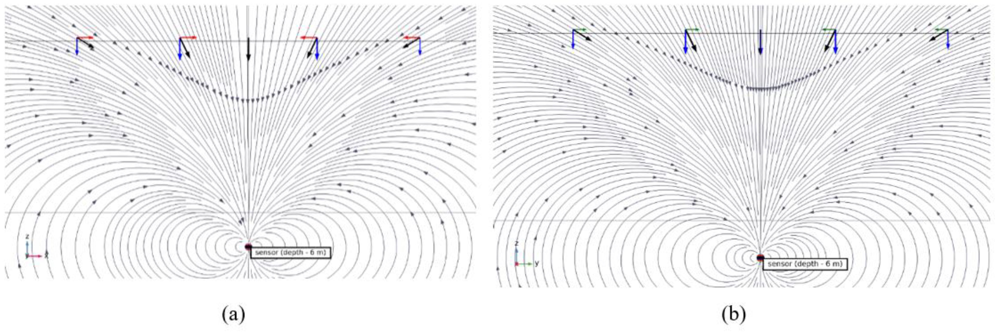
Figure 14 demonstrates that the resultant magnetic field strength vector unambiguously indicates the direction toward the radio beacon. The intersection of vectors approximately shows the location point of the radio beacon itself. However, to determine the precise coordinates of the radio beacon, it is necessary to apply the approaches presented above.
5. Conclusion
The studies conducted have shown that in the process of determining the coordinates of a radio beacon in a rock debris pile after blasting operations, there are error components that can be accounted for in calculations, as well as components that cannot be accounted for and can only be minimized. The unavoidable error is the coordinate inaccuracy caused by the tilt of the emitter axis. This error can be minimized through a design solution enabling adaptive vertical orientation of the emitter’s electromagnetic coil. Such an error may reach up to 3 meters, necessitating significant attention to this error type.
As demonstrated by the research, the error arising from rock heterogeneity, which depends on the presence of material lenses in the debris pile with varying electrical conductivity, is not substantial in most cases. This error should only be considered when the ore contains significant metal content or is saturated with highly mineralized groundwater.
The error dependent on the debris pile’s shape and the manifestation of a lateral magnetic field peak (in addition to the central peak) from a single emitter can be accurately determined using a specialized methodology for radio beacon search, lateral peak detection, and calculation of the main peak’s deviation from the radio beacon’s vertical axis.
The primary conclusion of the study is that precise determination of radio beacon coordinates requires the use of a loop-shaped receiving coil to capture the vertical component of the magnetic field strength, following the specified error-accounting rules. For approximate localization of the radio beacon, an additional receiver with three orthogonally positioned coils may be employed. This receiver can indicate the radio beacon’s location at the intersection point of magnetic field strength vectors.
An additional finding from the research indicates that radio beacons must be differentiated by frequency or digital identifiers, as field overlap and ambiguous peak determination may occur in certain cases.
Author Contributions
Conceptualization, A.S. and D.K.; methodology, A.S.; software, K.V.; validation, E.K., A.S. and D.K.; formal analysis, V.R.; investigation, E.K., A.S.; resources, D.K.; data curation, E.K.; writing—original draft preparation, E.K., A.S.; writing—review and editing, A.S.; visualization, E.K.; supervision, A.S.; project administration, D.K.; funding acquisition, A.S. All authors have read and agreed to the published version of the manuscript.
Funding
The research was supported by the Krasnoyarsk Regional Found of Science within the framework of the scientific project “Creation of a hardware and software complex for refining the component composition of broken-rock disintegration in the process of drilling and blasting operations based on the method of monitoring the boundaries of blocks with significantly different contents of useful components” (application number 20241018-08625).
Data Availability Statement
The presented research is original. All available materials are presented in this article. The materials of the article can be presented to the scientific community, can be placed in electronic sources. The calculation files do not represent scientific value. Therefore, the intermediate calculation materials are not presented in electronic resources on the Internet. Experimental studies are confirmed by photographic materials.
Conflicts of Interest
The authors declare no conflicts of interest. The funders had no role in the design of the study; in the collection, analyses, or interpretation of data; in the writing of the manuscript; or in the decision to publish the results.
Abbreviations
| MDPI | Multidisciplinary Digital Publishing Institute |
| DOAJ | Directory of open access journals |
| TLA | Three letter acronym |
| LD | Linear dichroism |
| N-S | From north to south |
| W-E | From west to east |
| BMM | Blast Movement Monitoring |
| DBO | Drilling and blasting operations |
| FEM | Finite element method |
References
- Adam, M; Thornton, D. A new technology for measuring blast movement. Innovative Mineral Development Symposium, Australian Institute of Mining and Metallurgy, 2004; Shore School, North Sydney, NSW, Australia; pp. 87–96.
- Engmann, E; Ako, S; Bisiaux, B; Rogers, W; Kanchibotla, S. Measurement and modelling of blast movement to reduce ore losses and dilution at Ahafo Gold Mine in Ghana, 2013; Ghana Min J. 14; pp. 27–36.
- Thornton, D. The application of electronic monitors to understand blast movement dynamics and improve blast designs, 2009b; In: JA Sanchidrian, editor. Proceedings of the Ninth International Symposium on Rock Fragmentation by Blasting – Fragblast 9. London: Taylor and Francis Group; pp. 287–399.
- Yennamani, AL. Blast induced rock movement measurement for grade control at the Phoenix mine [Masters Thesis], 2010; Department of Mining Engineering, Mackay school of Mines, Reno, University of Nevada; p. 123.
- Fitzgerald, M; York, S; Cooke, D; Thornton, D. Blast monitoring and blast translation–Case study of a grade improvement project at the Fimiston Pit, 2011; Kalgoorlie, Western Australia. Eighth International Mining Geology Conference, Queenstown, New Zealand; pp. 22–24.
- Gilbride, L; Taylor, S; Songlin, Z; Daemen, JJ; Mousset, JP. Blast-induced rock movement modelling for Nevada gold mines/ 1996; Int J Rock Mech Min Sci Geomech Abstr. 6; p. 270. [CrossRef]
- Loeb, J; Thornton, D. A cost benefit analysis to explore the optimal number of blast movement monitoring locations. 2014; Proceedings of the Ninth International Mining Geology Conference, Adelaide, SA, 18–21 August 2014: Australia Institute of Mining and Metallurgy; pp. 441–449.
- Câmara, T.R.; Leal, R.S.; Peroni, R.D.; Capponi, L.N. Controlling operational dilution in open-pit mining. 2019; Min Technol. 128; pp. 1–8. [CrossRef]
- La Rosa, D; Thornton, D. Blast movement modelling and measurement, 2011.; Proc. 35th Symp. Application of computers and operation research in the Minerals Industry (APCOM), Sep. 24-30, Wollongong, NSW, APCOM; pp.297-309.
- Firth, I.; Taylor, D. Bench blast modeling using numerical simulation and mine planning software. 2001; SME Annual Meeting. Feb. 26-28, Denver, USA; pp.01-40.
- Rogers, W.; et al. Understanding blast movement at Ahafo gold mine in Ghana, 2012; Proc. 38th Annual Conference on Explosives and Blasting Technique, Feb 12-15, Nashville, USA.
- Thornton, D.; Yennamanl, A.; Aquirre, S; Mousset-Jones, P. Blast-induced rock movement measurement for grade control, 2011; University of Nevada, Reno; 233 p.
- Patent US 7891233 B2. Blast movement monitor. No.: 11/556846. Feb. 22. 2011.
- Patent US 2007 /0151345 Al. Blast movement monitor. No.:11/556846. Jul. 5 2007.
- Pierre Mousset-Jones. Blast induced rock movement measurement for grade control at the phoenix mine, 2011; A thesis submitted in partial fulfillment of the requirements for the degree of Master of Science in Mining Engineering. University of Nevada, Reno; 245 р.
- Blakely, R.J. Potential Theory in Gravity and Magnetic Applications, 1995; Cambridge University Press.
- Sheinker et al. Localization in 2D using beacons of low frequency magnetic field. 2013; IEEE Journal of Selected Topics in Applied Earth Observations and Remote Sensing. 6(2); pp. 1020–1030. [CrossRef]
- Patent US 2007 /0151345 Al. Blast movement monitor. Appl. No. 11/556846. Nov. 6. 2006.
- Patent US 2005/0012499 A1. Blast movement monitor and method for determining the movement of а blast movement monitor and associated rock as а result of blasting operations. Appl. No. 10/854905. Мау 27. 2004.
- Demirchyan, K.S.; Neiman, L.R.; Korovkin, N.V.; Chechurin, V.L. Theoretical foundations of electrical engineering, 2003; In 3 volumes. Textbook for universities. Volume 3. – 4th ed. St. Petersburg: Piter; 377 p.
- do Amaral, P.A.; Borges, W.R.; Toledo, C.L.; Silva, A.M.; de Godoy, H.V.; Leão Santos, M.H. Electrical Prospecting of Gold Mineralization in Exhalites of the Digo-Digo VMS Occurrence, 2023; Central Brazil. Minerals, 13; p. 1483. [CrossRef]
- Gromova, M.P.; Varenichev, A.A.; Komogortsev, B.V. Raw material base of gold in Russia, 2016; Mining information and analytical bulletin (scientific and technical journal).. No. 8.; pp. 212-220.
- Zhdanov, M.S.; Velikhov, E.P. Geophysical electromagnetic theory and methods, 2012; Trans. from English / Ed. Moscow: Scientific world. 680 p.
Figure 1.
Internal structure of BMM sensors.
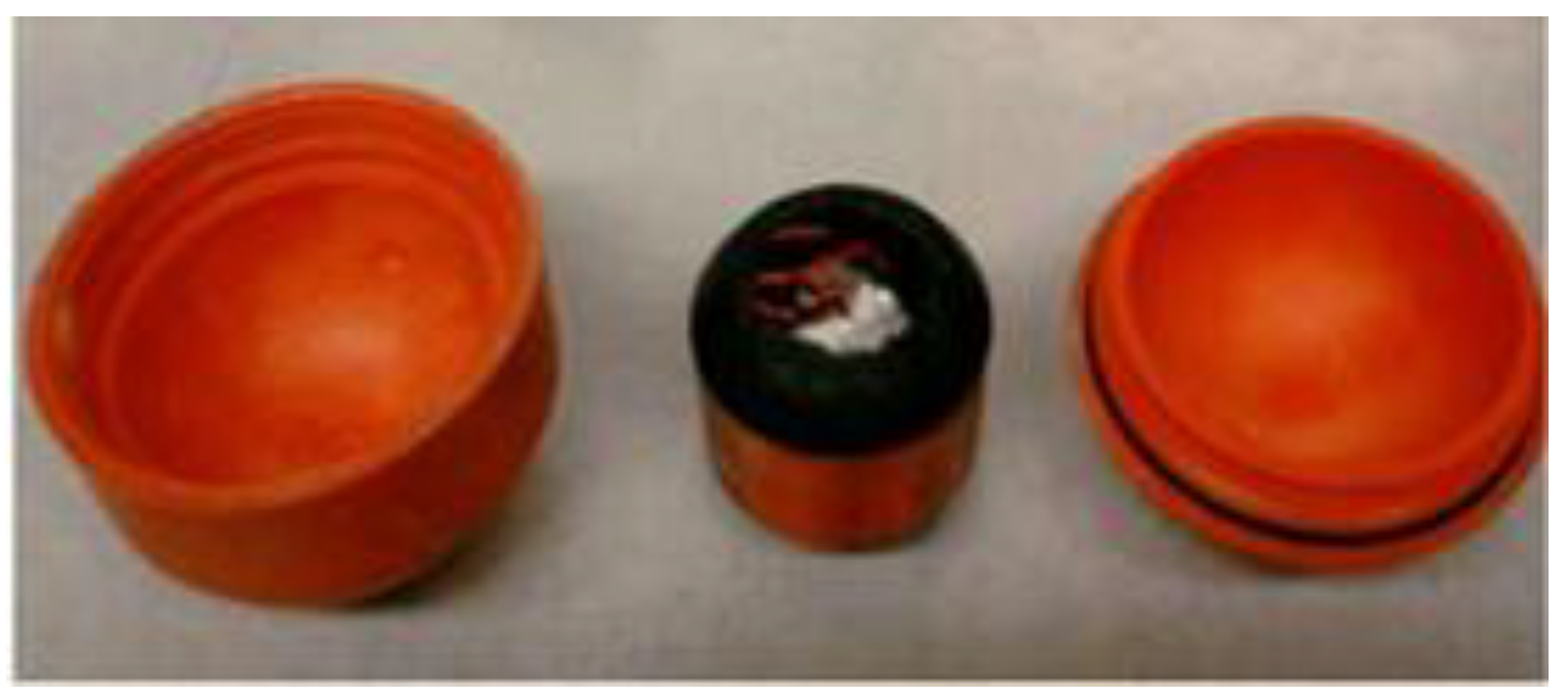
Figure 2.
Magnetic dipole field: (a) Schematic representation; (b) Model representation of the magnetic field lines and the distribution of its axial component Hz.
Figure 2.
Magnetic dipole field: (a) Schematic representation; (b) Model representation of the magnetic field lines and the distribution of its axial component Hz.
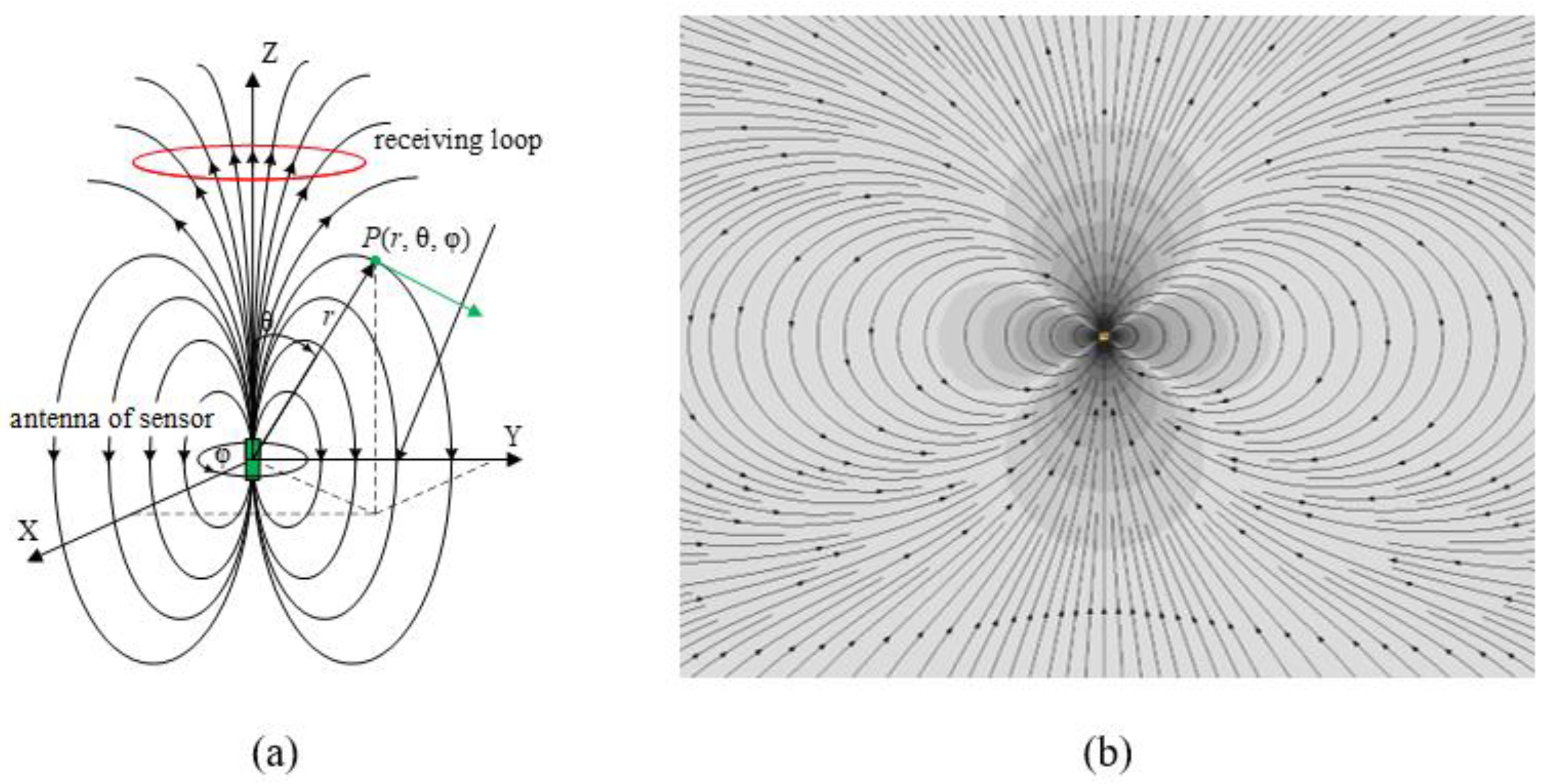
Figure 3.
Schematic diagram of a model of a section of rocks with a flat surface including a low-resistivity anomaly.
Figure 3.
Schematic diagram of a model of a section of rocks with a flat surface including a low-resistivity anomaly.
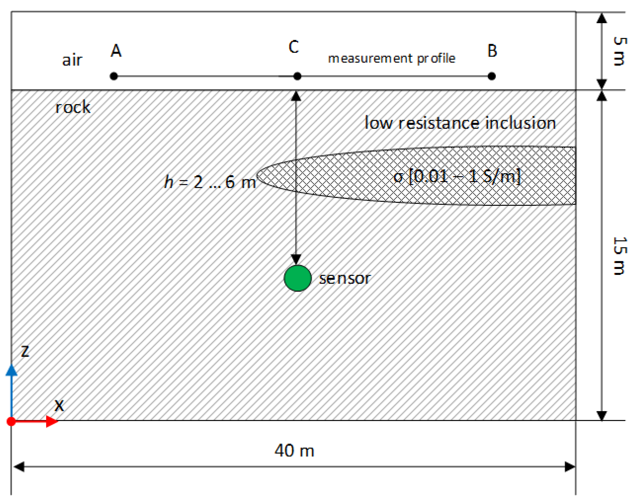
Figure 4.
Schematic of the rock debris model and sensor placement.
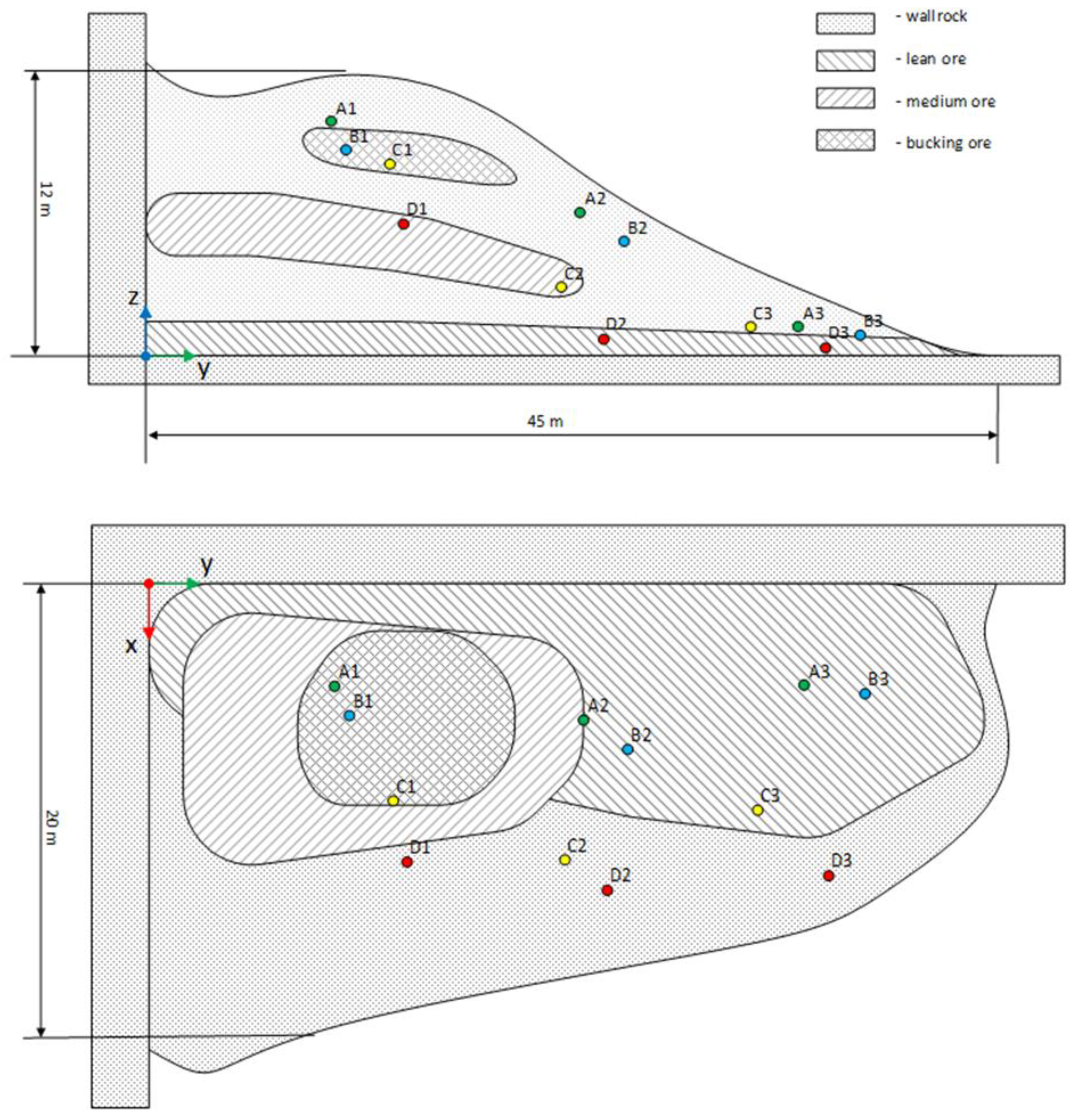
Figure 5.
The level of the axial component of the magnetic field along the profile on the model surface for depths of 2–6 m.
Figure 5.
The level of the axial component of the magnetic field along the profile on the model surface for depths of 2–6 m.
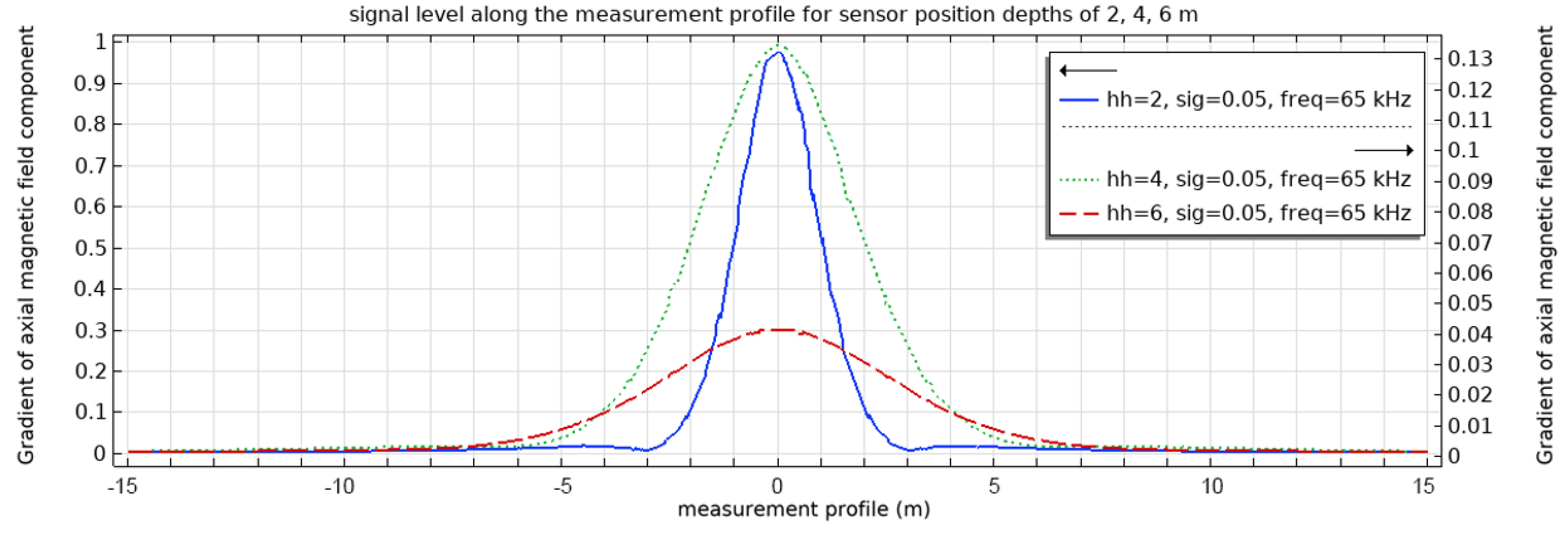
Figure 6.
Level of the axial component of the magnetic field along the profile on the model surface for a sensor depth of 6 m with shielding by a low-resistance inclusion at varying electrical conductivities.
Figure 6.
Level of the axial component of the magnetic field along the profile on the model surface for a sensor depth of 6 m with shielding by a low-resistance inclusion at varying electrical conductivities.
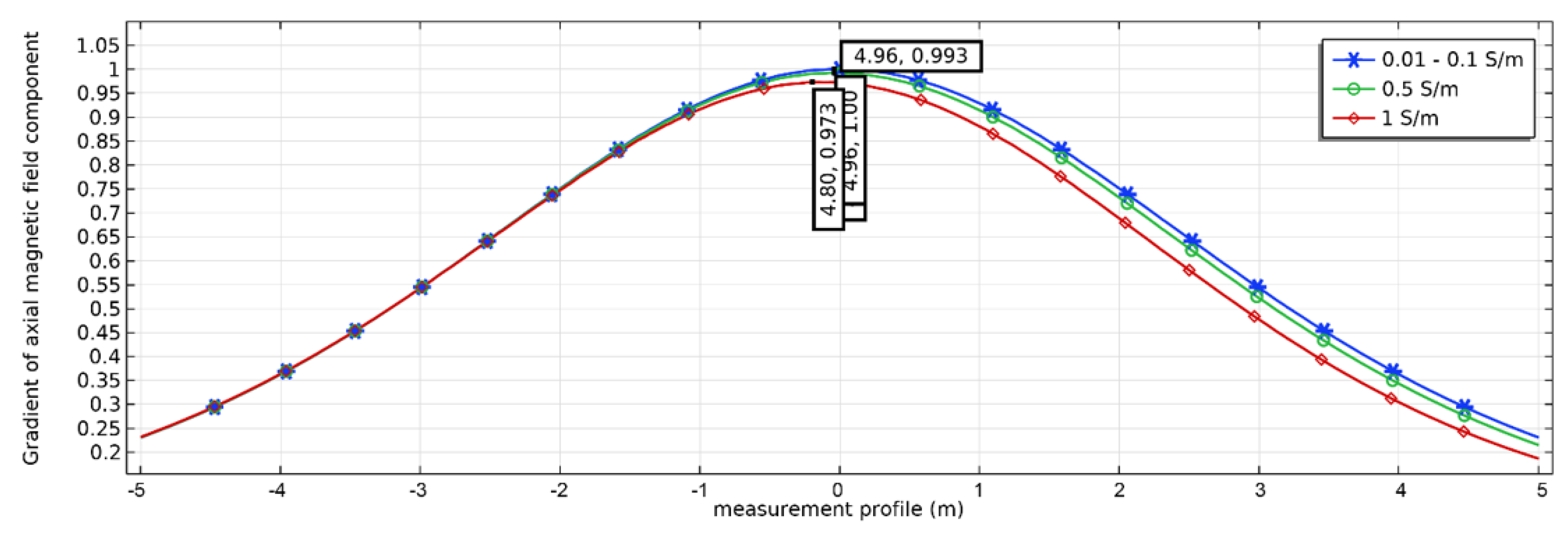
Figure 7.
Dependence of the axial component level of the magnetic field on distance: (a) Section 0–6.5 m; (b) Section 5–6.5 m.
Figure 7.
Dependence of the axial component level of the magnetic field on distance: (a) Section 0–6.5 m; (b) Section 5–6.5 m.
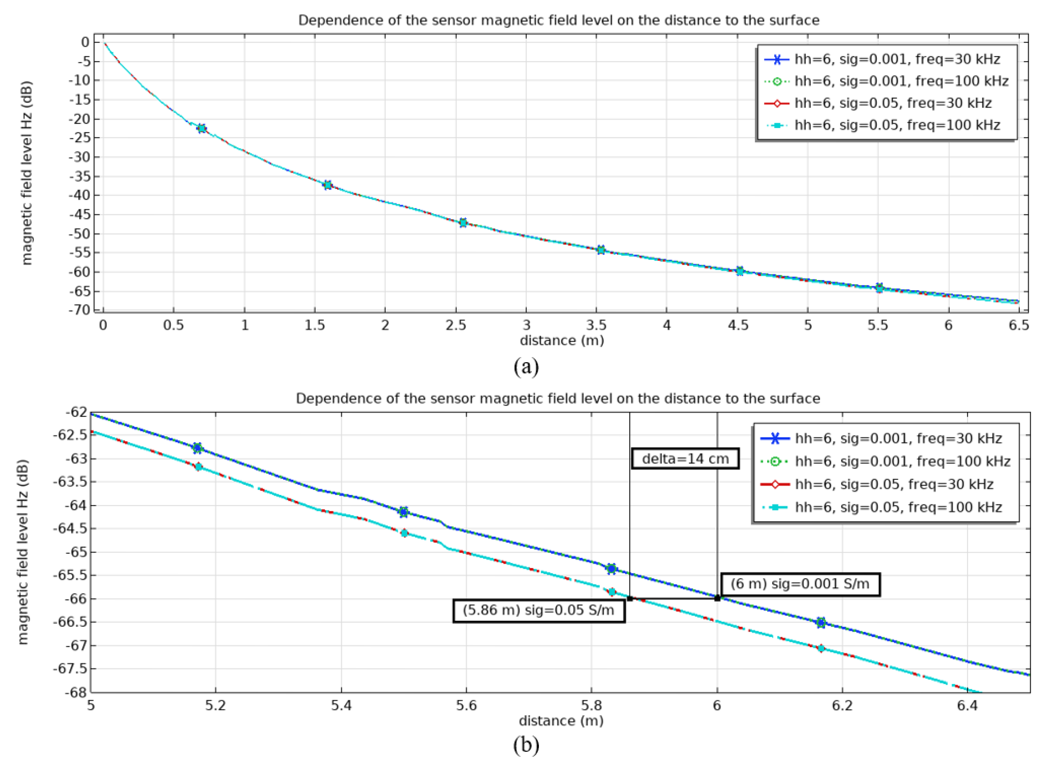
Figure 8.
Distribution of the vertical magnetic field level of a dipole at h = 6 m on the surface during its rotation by angle α: a – 0°; b – 45°; c – 90°.
Figure 8.
Distribution of the vertical magnetic field level of a dipole at h = 6 m on the surface during its rotation by angle α: a – 0°; b – 45°; c – 90°.
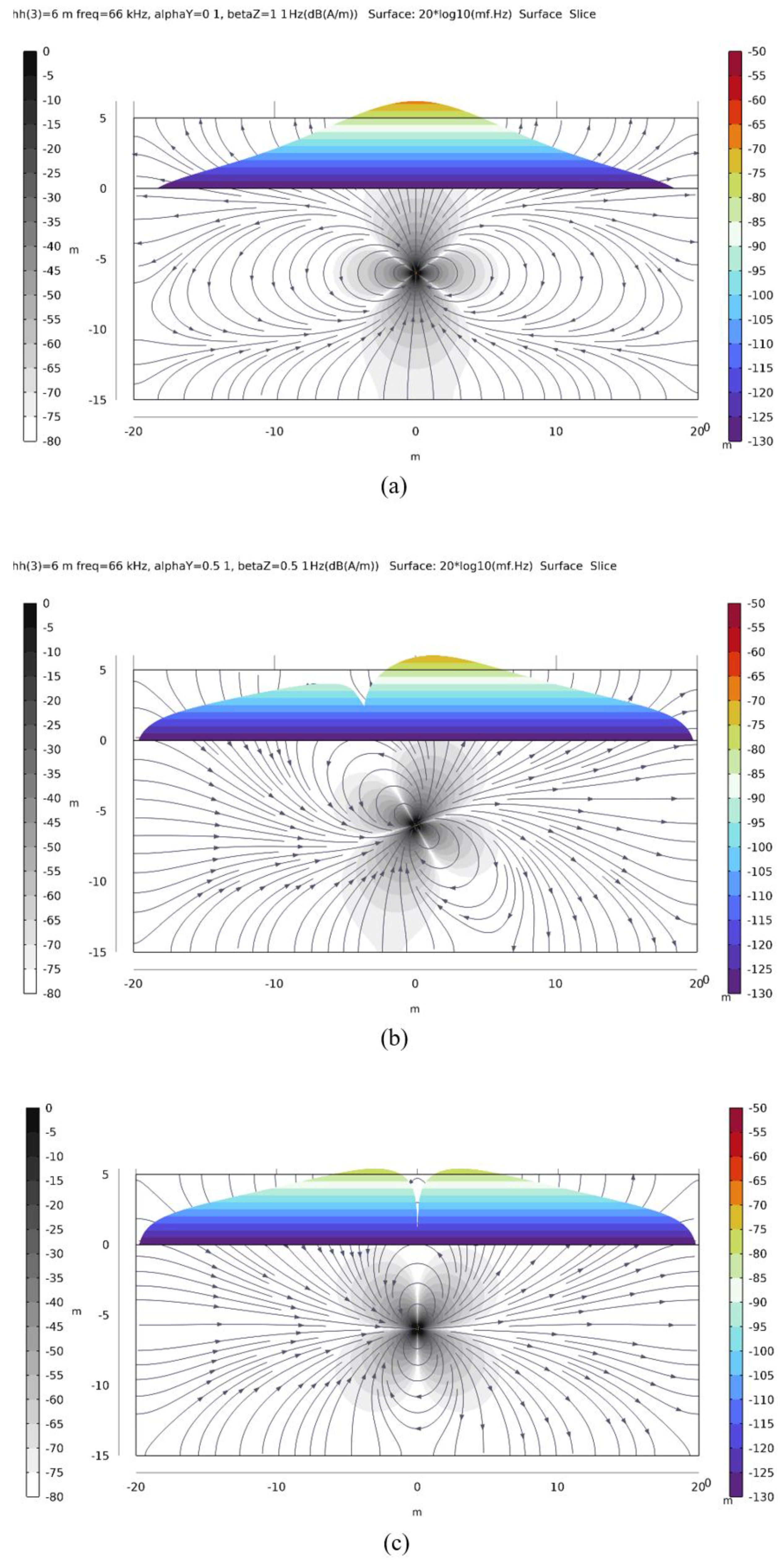
Figure 9.
Distribution of the vertical component of the magnetic field along the XZ profile during sensor antenna rotation at an angle α for depth positions: (a) h = 2 m; (b) h = 6 m.
Figure 9.
Distribution of the vertical component of the magnetic field along the XZ profile during sensor antenna rotation at an angle α for depth positions: (a) h = 2 m; (b) h = 6 m.
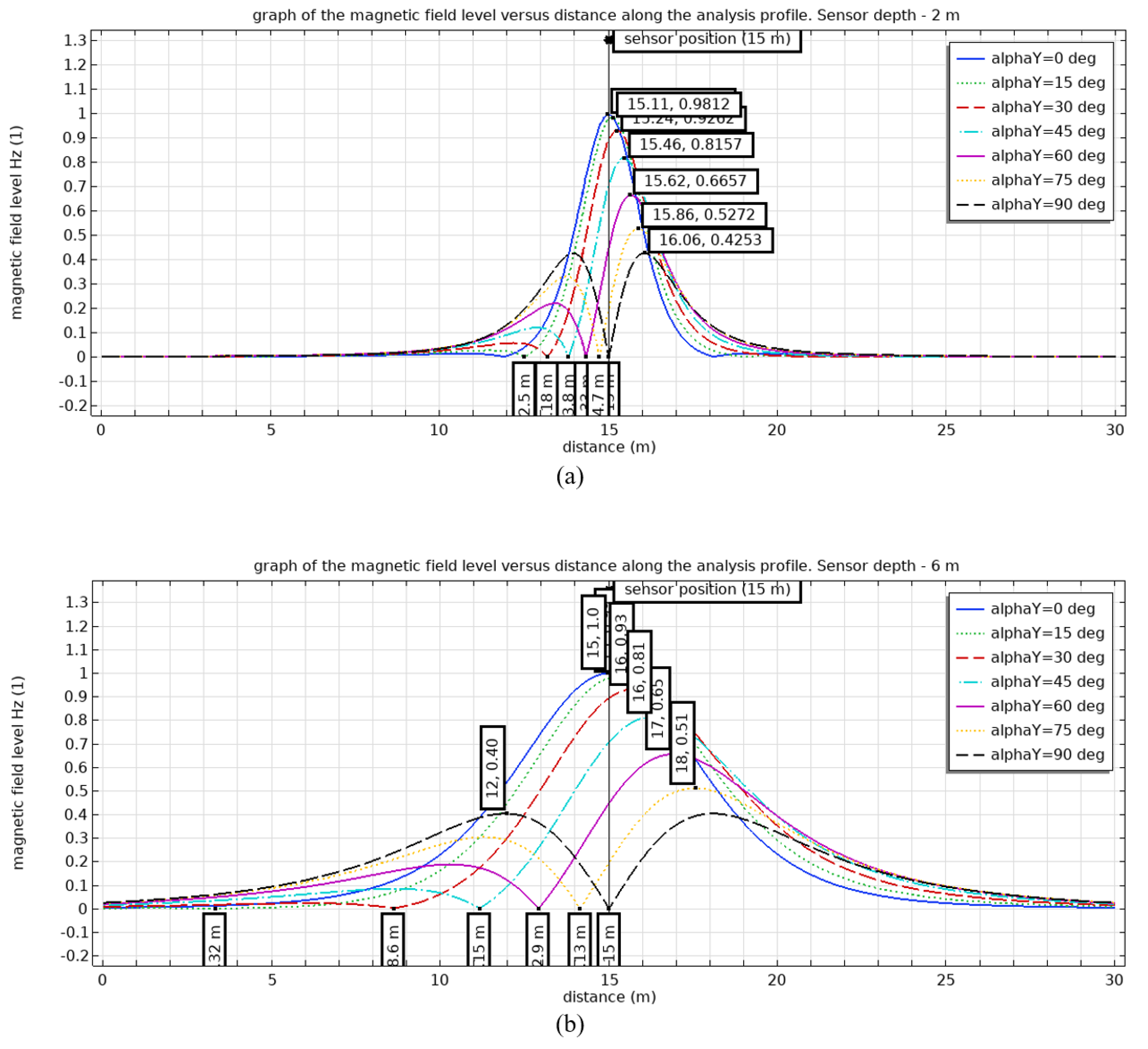
Figure 10.
Model of vertical magnetic field distribution on the surface of a rock debris pile: (a) Top view; (b) Isometric view.
Figure 10.
Model of vertical magnetic field distribution on the surface of a rock debris pile: (a) Top view; (b) Isometric view.
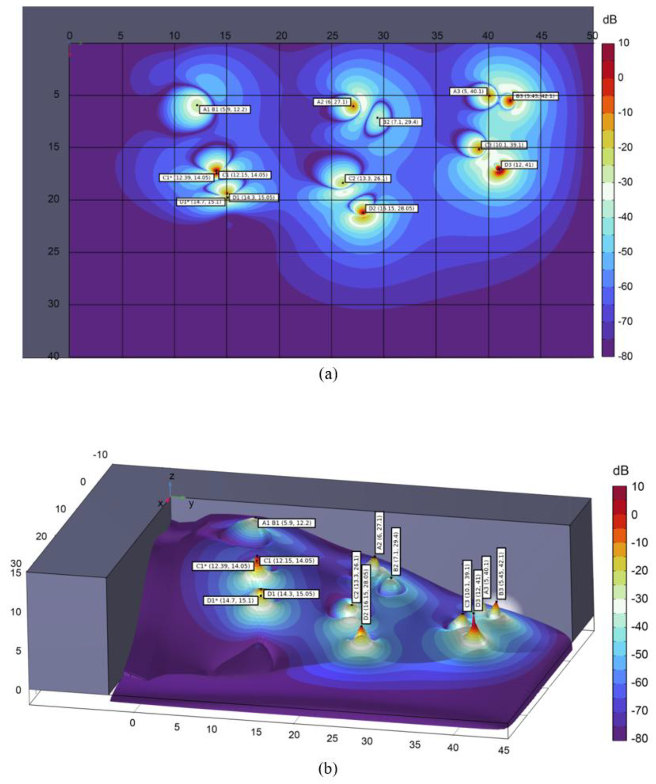
Figure 11.
Distribution of the axial component of the magnetic field beneath the observation profile: (a) Beneath flat terrain (sensor A2); (b) Beneath sloped terrain (sensor C1).
Figure 11.
Distribution of the axial component of the magnetic field beneath the observation profile: (a) Beneath flat terrain (sensor A2); (b) Beneath sloped terrain (sensor C1).
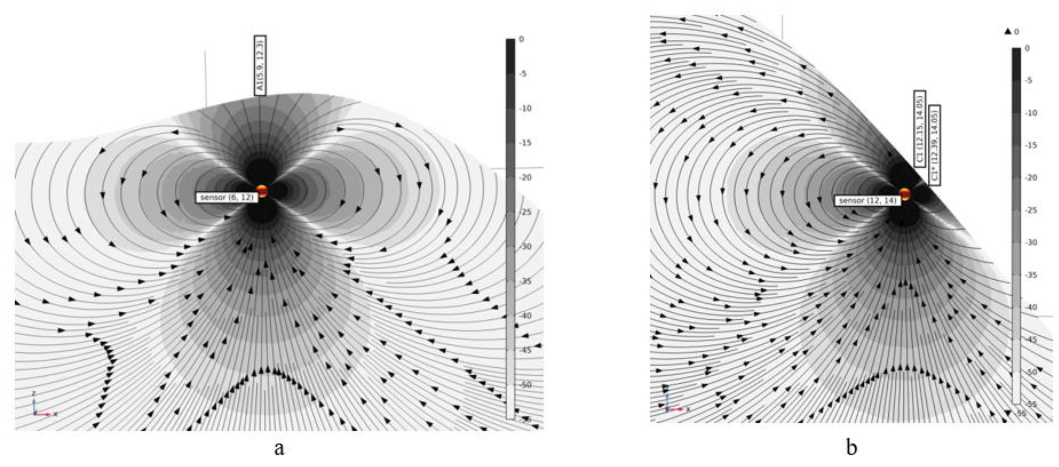
Figure 12.
Determination of the magnitude of the error in emitter coordinate determination during separate (a) and simultaneous (b) operation of emitters.
Figure 12.
Determination of the magnitude of the error in emitter coordinate determination during separate (a) and simultaneous (b) operation of emitters.
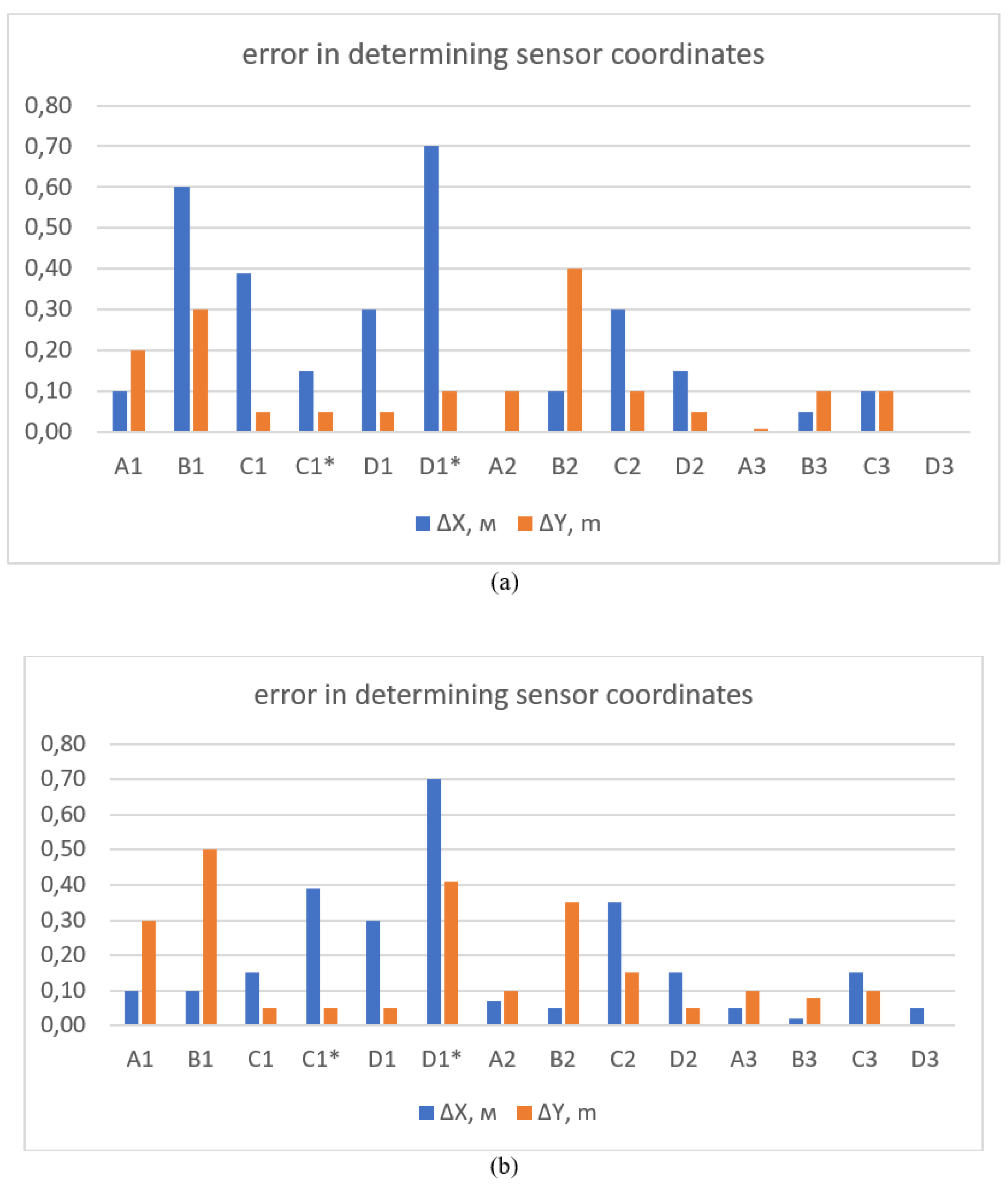
Figure 14.
Determination of the radio beacon search direction using the resultant magnetic field strength vector of the emitter.
Figure 14.
Determination of the radio beacon search direction using the resultant magnetic field strength vector of the emitter.
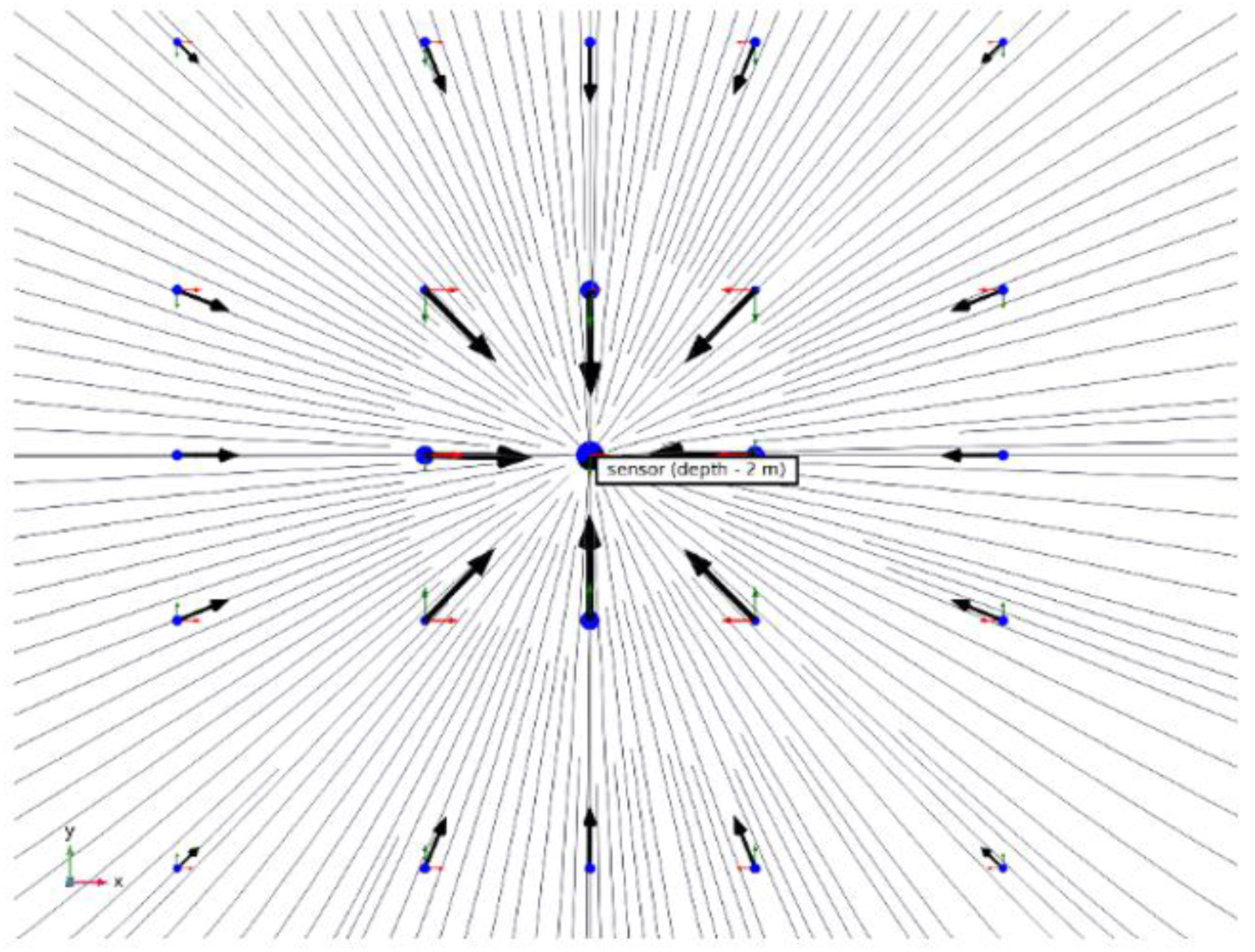

Table 1.
Petrophysical properties of rocks for the model.
| Name of rocks | Electrical conductivity σ, S/m | Relative permittivity ε |
|---|---|---|
| wallrock | 0.001 | 8 |
| lean ore | 0.005 | 10 |
| medium ore | 0.01 | 12 |
| bucking ore | 0.05 | 13 |
Table 2.
Coordinates of the position of sensors in the rock collapse model.
| Sensor name | Coordinates, m | |
|---|---|---|
| X | Y | |
| A1 | 6 | 12 |
| B1 | 6.5 | 12.5 |
| C1 | 12 | 14 |
| D1 | 14 | 15 |
| A2 | 6 | 27 |
| B2 | 7 | 29 |
| C2 | 13 | 26 |
| D2 | 16 | 28 |
| A3 | 5 | 40 |
| B4 | 5.5 | 42 |
| C5 | 10 | 39 |
| D5 | 12 | 41 |
Disclaimer/Publisher’s Note: The statements, opinions and data contained in all publications are solely those of the individual author(s) and contributor(s) and not of MDPI and/or the editor(s). MDPI and/or the editor(s) disclaim responsibility for any injury to people or property resulting from any ideas, methods, instructions or products referred to in the content. |
© 2025 by the authors. Licensee MDPI, Basel, Switzerland. This article is an open access article distributed under the terms and conditions of the Creative Commons Attribution (CC BY) license (http://creativecommons.org/licenses/by/4.0/).
Copyright: This open access article is published under a Creative Commons CC BY 4.0 license, which permit the free download, distribution, and reuse, provided that the author and preprint are cited in any reuse.


