Manifolds of Product States of Three Qubits

1. Introduction

The concept of quantum entanglement was first introduced by Erwin Schrödinger in 1935, who referred to it as "Verschränkung" in German—a term that was later translated to "entanglement"—during the early development of quantum mechanics. Einstein, Podolsky and Rosen identified it as a fundamental aspect of quantum mechanics that remains central to modern physics [1,2]. They highlighted the existence of global states in composite systems that cannot be expressed as a simple product of the states of their individual parts. This phenomenon, entanglement, reveals an inherent structure in the statistical relationships between the components of a quantum system. It plays a pivotal role in quantum information theory and serves as a valuable resource for quantum communication and information processing [3,4,5]. For a product state ${\rho }_{A{\rm B}}$ of two subsystems ${\rho }_A$ and ${\rho }_B$ we have ${\rho }_{AB}={\rho }_A\otimes {\rho }_B$. For these states and only for these, the two subsystems, when described separately, provide a complete description of the composite system. Any state that is not a product state exhibits some form of correlation and is referred to as a correlated state. Quantum mechanics reveals that correlations come in a hierarchy, with distinct physical properties emerging at different levels. The simplest among these are classically correlated, or separable, states. These states have density matrices that can always be expressed in the following form:

$$\rho ={{\displaystyle \sum }}_i{p}_i{\rho }_{Ai}\otimes {\rho }_{Bi}\mathrm{with}0\le p_i\le 1\mathrm{and}{{\displaystyle \sum }}_i{p}_i=1$$

(1)

that is, a convex mixture of product states. Although a density matrix may be known to represent a separable system, no general algorithm exists for decomposing it according to Eq. (1), and such a decomposition is not unique. Peres and the Horodecki family [6,7] provided a mathematical characterization of these states—at least in the specific cases where the composite Hilbert space has dimensions 2×2 or 2×3. States that cannot be expanded in the form of eq. (1) are called “entangled”.

When exploring entanglement and related topics, it quickly becomes evident that geometry plays a crucial role, often providing a highly intuitive and vivid understanding of these concepts. The goal of this work is to identify the manifolds of product states for a system of three qubits. As a result, separable states can be expressed as convex combinations of these product states and every state that is not separable is entangled.

We begin with the Fano form of a density matrix, a density matrix of three qubits [8]. In this case we have totally product states ${\rho }_{ABC}={\rho }_A\otimes {\rho }_B\otimes {\rho }_C$, biproduct states ${\rho }_{IJK}={\rho }_{IJ}\otimes {\rho }_K$ for $\left(I,J,K\right)$ permutations of $\left(A,B,C\right)$, convex combinations of these and genuinely entangled states. Convex combinations of totally product states give totally separable states and of biproduct states give biseparable states [9].

The paper is organized as follows. Section 2 provides a review of essential concepts from geometry that are foundational for the subsequent analysis. In Section 3, we present our main results. Specifically, Section 3.1 discusses the Bloch vector representation for a single qubit. Section 3.2 introduces the Fano form for systems of two and three qubits and formulates two systems of equations characterizing biproduct and fully product states. Section 3.3 and Section 3.4 are devoted to solving these systems and identifying the associated manifolds. For biproduct states, we also compute the curvature of the corresponding manifold. The paper concludes with a discussion in Section 4, highlighting directions for future research.

2. Preliminary Issues (Geometry)

Let us consider the n-dimensional manifold ${\mathbb{R}}^n$ and the m-dimensional manifold ${\mathbb{R}}^m$ with $m<n$. Let $F:{\mathbb{R}}^m\to {\mathbb{R}}^n$ be a $C^{\infty }$ function such that $F$ is an injection and an immersion, that is an embedding. Then $M=F\left({\mathbb{R}}^m\right)$ is a submanifold of ${\mathbb{R}}^n$ [10].

The manifold ${\mathbb{R}}^n$ admits a natural metric called “Euclidian” $h={\delta }_{\alpha \beta }d{x}^{\alpha }\otimes d{x}^{\beta }$ where $\alpha ,\beta =0,\dots ,n-1$, the Eistein summation convention is supposed and

$${\delta }_{\alpha \beta }=\left\{\begin{array}{c}1 if \alpha =\beta \\ 0 if \alpha \ne \beta \end{array}\right.$$

(2)

is the Kronecker delta. This means that if we make an infinitesimal step into ${\mathbb{R}}^n$ that is $x^{\alpha }\to x^{\alpha }+d{x}^{\alpha }$ then the length of this step is $ds$ where $d{s}^2={\delta }_{\alpha \beta }d{x}^{\alpha }\otimes d{x}^{\beta }$. If we are on a 2D flat surface we know this as “Pythagorean” theorem. In ${\mathbb{R}}^m$ we have an induced metric $g=F^{*}h$ i.e.

$$g=g_{\mu \nu }d{u}^{\mu }\otimes d{u}^{\nu }$$

(3)

with [10]

$$g_{\mu \nu }={\delta }_{\alpha \beta }{\displaystyle \frac{𝜕F^{\alpha }}{𝜕u^{\mu }}}{\displaystyle \frac{𝜕F^{\beta }}{𝜕u^{\nu }}}$$

(4)

and $\mu ,\nu =0,\dots ,m-1.$ Correspondingly, if we make an infinitesimal step into ${\mathbb{R}}^m$ such that $u^{\mu }\to u^{\mu }+d{u}^{\mu }$ then the length will be $ds$with

$$d{s}^2=g_{\mu \nu }d{u}^{\mu }\otimes d{u}^{\nu }$$

(5)

For the manifold $M$ we may compute the connection coefficients ${\Gamma }_{ \mu \nu }^{\lambda }$ of the Levi-Civita connection

$${\Gamma }_{ \mu \nu }^{\lambda }={\displaystyle \frac{1}{2}}{g}^{\lambda \kappa }\left({\displaystyle \frac{𝜕g_{\nu \kappa }}{𝜕u^{\mu }}}+{\displaystyle \frac{𝜕g_{\mu \kappa }}{𝜕u^{\nu }}}-{\displaystyle \frac{𝜕g_{\mu \nu }}{𝜕u^{\kappa }}}\right)$$

(6)

and subsequently the Riemann curvature tensor

$$R_{ \lambda \mu \nu }^{\kappa }={\displaystyle \frac{𝜕{\Gamma }_{ \nu \lambda }^{\kappa }}{𝜕u^{\mu }}}-{\displaystyle \frac{𝜕{\Gamma }_{ \mu \lambda }^{\kappa }}{𝜕u^{\nu }}}+{\Gamma }_{ \nu \lambda }^{\eta }{\Gamma }_{ \mu \eta }^{\kappa }-{\Gamma }_{ \mu \lambda }^{\eta }{\Gamma }_{ \nu \eta }^{\kappa }$$

(7)

the Ricci tensor

$$R_{\mu \nu }=R_{ \mu \lambda \nu }^{\lambda }$$

(8)

and the scalar curvature

$$Q=g^{\mu \nu }{R}_{\mu \nu }$$

(9)

3. Results

3.1. Bloch Sphere Expansion Form of One Qubit

Let ${\rho }_A$ be the density matrix of one qubit. Then we can expand it

$${\rho }_A={\displaystyle \frac{1}{2}}\left(I_2+a_1{\sigma }^1+a_2{\sigma }^2+a_3{\sigma }^3\right)$$

(10)

where $I_2$ is the identity matrix, ${\sigma }^i$, $i=1,2,3$, are the Pauli matrices and if $\overrightarrow{a}=\left(a_1,a_2,a_3\right)$ is the radius of the so-called Bloch sphere, $\left|\overrightarrow{a}\right|\le 1$. That means that we have a base given by the “vectors” $\left(e^0,e^1,e^2,e^3\right)={\displaystyle \frac{1}{2}}\left(I_2,{\sigma }^1,{\sigma }^2,{\sigma }^3\right)$ since it is easy to check that $tr\left(e^i·e^j\right)={\displaystyle \frac{1}{2}}{\delta }_{ij}$.

3.2. Fano Form of Two and Three Qbits

If ${\rho }_{AB}$ is a density matrix of two qubits, we have the Fano form expansion [8]

$${\rho }_{AB}={\displaystyle \sum }_{i,j=0}^3{a}_{ij}{e}^i\otimes e^j$$

(11)

with $a_{ij}ϵ\mathbb{R}$ and such that ${\rho }_{AB}$ is a density matrix. For three qubits

$${\rho }_{ABC}={\displaystyle \sum }_{i,j,k=0}^3{d}_{ijk}{e}^i\otimes e^j\otimes e^k$$

(12)

Again $d_{ijk}ϵ\mathbb{R}$ and such that ${\rho }_{ABC}$ is a density matrix.

In case of a biproduct state ${\rho }_{ABC}={\rho }_{AB}\otimes {\rho }_C$, given the expansions (11), (12) and one for ${\rho }_C=\sum c_i{e}^i$, we have

$$a_{ij}{c}_k=d_{ijk}$$

(13)

for $i,j,k=0,\dots ,3$ and similarly for the other cases ${\rho }_{AC}\otimes {\rho }_B$ or ${\rho }_{BC}\otimes {\rho }_A$. In case of a product state ${\rho }_{ABC}={\rho }_A\otimes {\rho }_B\otimes {\rho }_C$ we have

$$a_i{b}_j{c}_k=d_{ijk}$$

(14)

where

$${\rho }_A={\displaystyle \sum }_{i=0}^3{a}_i{e}^i, {\rho }_B={\displaystyle \sum }_{i=0}^3{b}_i{e}^i, {\rho }_C={\displaystyle \sum }_{i=0}^3{c}_i{e}^i$$

(15)

3.3. Solving the System for a Biproduct State

The system we want to solve is the system (13) for $a_{00}=c_0=d_{000}=1$. It is obvious that its solution is

$$\begin{gathered} a_{ij}=d_{ij0}\mathrm{for}i,j=0,1,2,3 \\ {c}_k=d_{00k}\mathrm{for}k=0,1,2,3 \end{gathered}$$

(16)

But we have to impose the conditions

$$d_{00k}{d}_{ij0}=d_{ijk}\mathrm{for}i,j,k=0,1,2,3$$

(17)

Now, let $K$ be the function

$$K:\left(d_{00k},d_{ij0}\right)\mapsto \left(d_{00k},d_{ij0},d_{ij1},d_{ij2},d_{ij3}\right)$$

(18)

defined by relations (17) for $k=1,2,3$ and $i,j=0,1,2,3$ except for the case $i=j=0$. To be precise the order of the coordinates of the domain of $K$ is

$$\left(d_{001},d_{002},d_{003}, d_{010},d_{020},d_{030},d_{100},d_{110},d_{120},d_{130},d_{200},d_{210},d_{220},d_{230},d_{300},d_{310},d_{320},d_{330}\right)$$

and for the image

$$\begin{gathered} (d_{001},d_{002},d_{003}, d_{010},d_{020},d_{030},d_{100},d_{110},d_{120},d_{130},d_{200},d_{210},d_{220},d_{230},d_{300},d_{310},d_{320},d_{330}, \\ {d}_{011},d_{012},d_{013},d_{021},d_{022},d_{023},d_{031},d_{032},d_{033},d_{101},d_{102},d_{103},d_{111},d_{112},d_{113},d_{121},d_{122},d_{123}, \\ {d}_{131},d_{132},d_{133},d_{201},d_{202},d_{203},d_{211},d_{212},d_{213},d_{221},d_{222},d_{223}, d_{231},d_{232},d_{233},d_{301},d_{302},d_{303}, \\ {d}_{311},d_{312},d_{313},d_{321},d_{322},d_{323},d_{331},d_{332},d_{333}) \end{gathered}$$

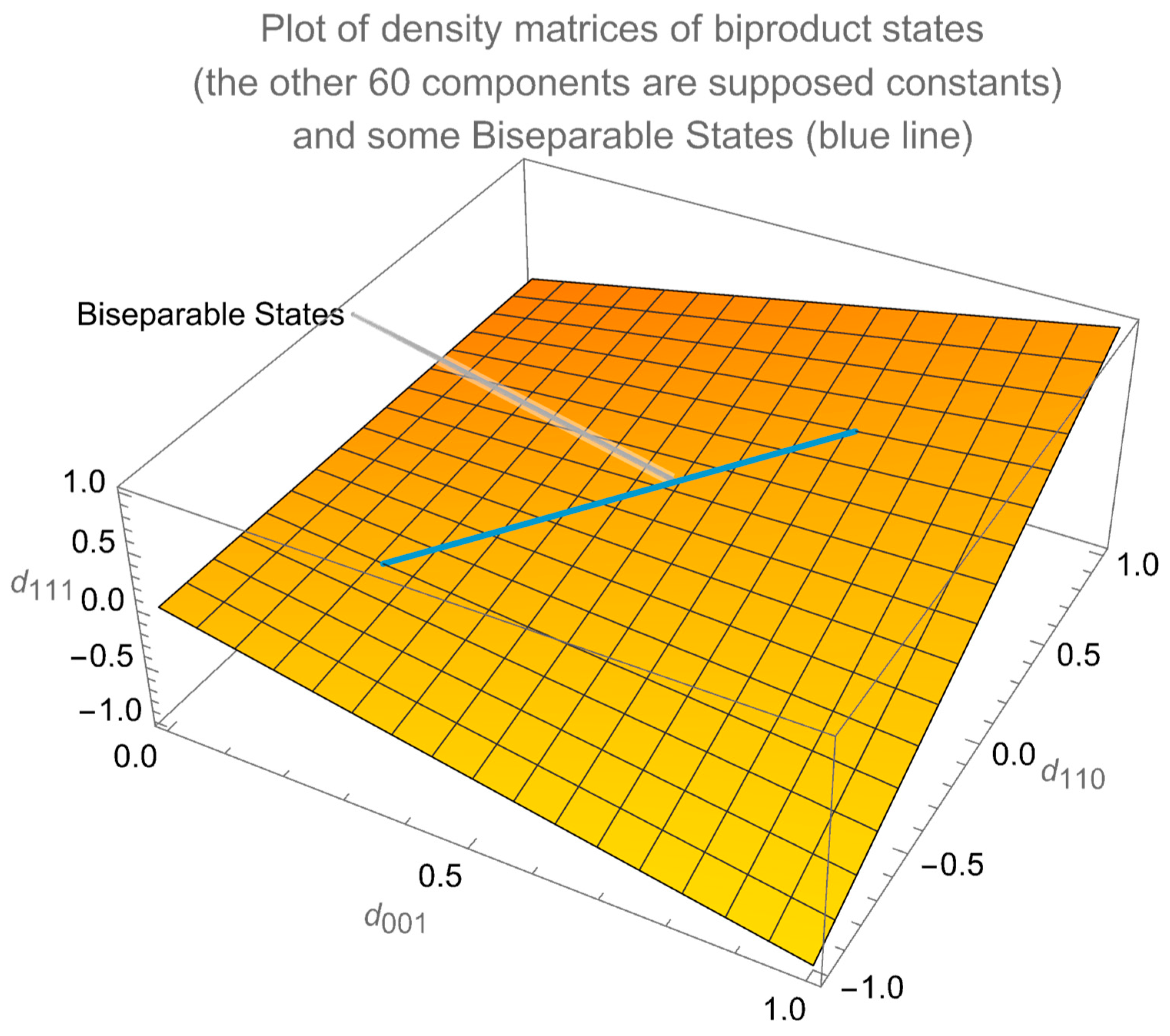
We notice that $K$ is a $C^{\infty }$ function from ${\mathbb{R}}^{18}$ to ${\mathbb{R}}^{63}$. So, we have an 18-dimensional (hyper)surface $S$ embedded in the 63-dimensional manifold ${\mathbb{R}}^{63}$. The (hyper)surface $S$ is a manifold of biproduct states into the whole space of tripartite density matrices.

If $h$ is the Euclidian metric in ${\mathbb{R}}^{63}$ we can compute the induced metric $g=K^{*}h$. The result is (eq. (4))

$$\begin{gathered} g_{\mu \mu }={{\displaystyle \sum }}_{i,j=0}^3{d}_{ij0}^2\mathrm{for}\mu =0,1,2 \\ {g}_{\mu \mu }={{\displaystyle \sum }}_{i=0}^3{d}_{00i}^2\mathrm{for}\mu =3, \dots ,17 \\ {g}_{\mu \nu }=d_{00\nu }{m}_{\mu -2}\mathrm{for}\mu =3, \dots ,17,\mathrm{\nu }=0,1,2 \\ {g}_{\nu \mu }=g_{\mu \nu } \end{gathered}$$

(19)

where $\overrightarrow{m}=\left(m_0,\dots ,m_{15}\right)=\left(a_{00},a_{01},\dots ,a_{32},a_{33}\right)=\left(d_{000},d_{010},\dots ,d_{320},d_{330}\right)$ a vector made from matrix $a$. The other components of $g$ are 0.

Then we procced computing the connection coefficients of the Levi-Civita connection (eq. (6)) the Riemann and Ricci tensors and finally the scalar curvature. Using “mathematica” we have for the scalar curvature $Q$:

$$\begin{gathered} q_1={{\displaystyle \sum }}_{i=1}^3{d}_{00i}^2 \\ {q}_2=1+q_1+{{\displaystyle \sum }}_{i=1}^3{d}_{0i0}^2+{{\displaystyle \sum }}_{i=1}^3{{\displaystyle \sum }}_{j=0}^3{d}_{ij0}^2 \\ Q=-{\displaystyle \frac{2\left(q_1-3q_2\right)\left(1+q_1+14q_2\right)}{(1+q_1)\left(q_1-q_2\right)q_2^2}} \end{gathered}$$

(20)

Since $q_1-q_2<0$and $q_1<3q_2$. we have

$$Q<0$$

Figure 1. The function $z=xy$ is plotted to illustrate biproduct states, assuming $x$ and $y$ correspond to elements of the associated density matrices.

Figure 1. The function $z=xy$ is plotted to illustrate biproduct states, assuming $x$ and $y$ correspond to elements of the associated density matrices.

3.4. Solving the System for a Product State

The system we want to solve is the system (14) for $a_0=b_0=c_0=d_{000}=1$. It is obvious that its solution is

$$\begin{gathered} a_i=d_{i00}\mathrm{for}i=0,1,2,3 \\ {b}_j=d_{0j0}\mathrm{for}j=0,1,2,3 \\ {c}_k=d_{00k}\mathrm{for}k=0,1,2,3 \end{gathered}$$

(21)

with the following conditions to be fulfilled

$$d_{i00}{d}_{0j0}{d}_{00k}=d_{ijk}\mathrm{for}i,j,k=0,1,2,3$$

(22)

Correspondingly $L$ will be the function

$$L:\left(d_{i00},d_{0j0},d_{00k}\right)\mapsto \left(d_{ijk}\right)$$

(23)

defined by relations (22) for $i,j,k=1,2,3$ (the domain) and $i,j,k=0,1,2,3$ for the image except for the case $i=j=k=0$.

To be precise again the order of the coordinates of the domain of $L$ is

$$\left(d_{100},d_{200},d_{300}, d_{010},d_{020},d_{030},d_{001},d_{002},d_{003}\right)$$

and for the image

$$\begin{gathered} (d_{001},d_{002},d_{003}, d_{010},d_{020},d_{030},d_{100},d_{110},d_{120},d_{130},d_{200},d_{210},d_{220},d_{230},d_{300},d_{310},d_{320},d_{330}, \\ {d}_{011},d_{012},d_{013},d_{021},d_{022},d_{023},d_{031},d_{032},d_{033},d_{101},d_{102},d_{103},d_{111},d_{112},d_{113},d_{121},d_{122},d_{123}, \\ {d}_{131},d_{132},d_{133},d_{201},d_{202},d_{203},d_{211},d_{212},d_{213},d_{221},d_{222},d_{223}, d_{231},d_{232},d_{233},d_{301},d_{302},d_{303}, \\ {d}_{311},d_{312},d_{313},d_{321},d_{322},d_{323},d_{331},d_{332},d_{333}) \end{gathered}$$

the same as the coordinates in case of $K$.

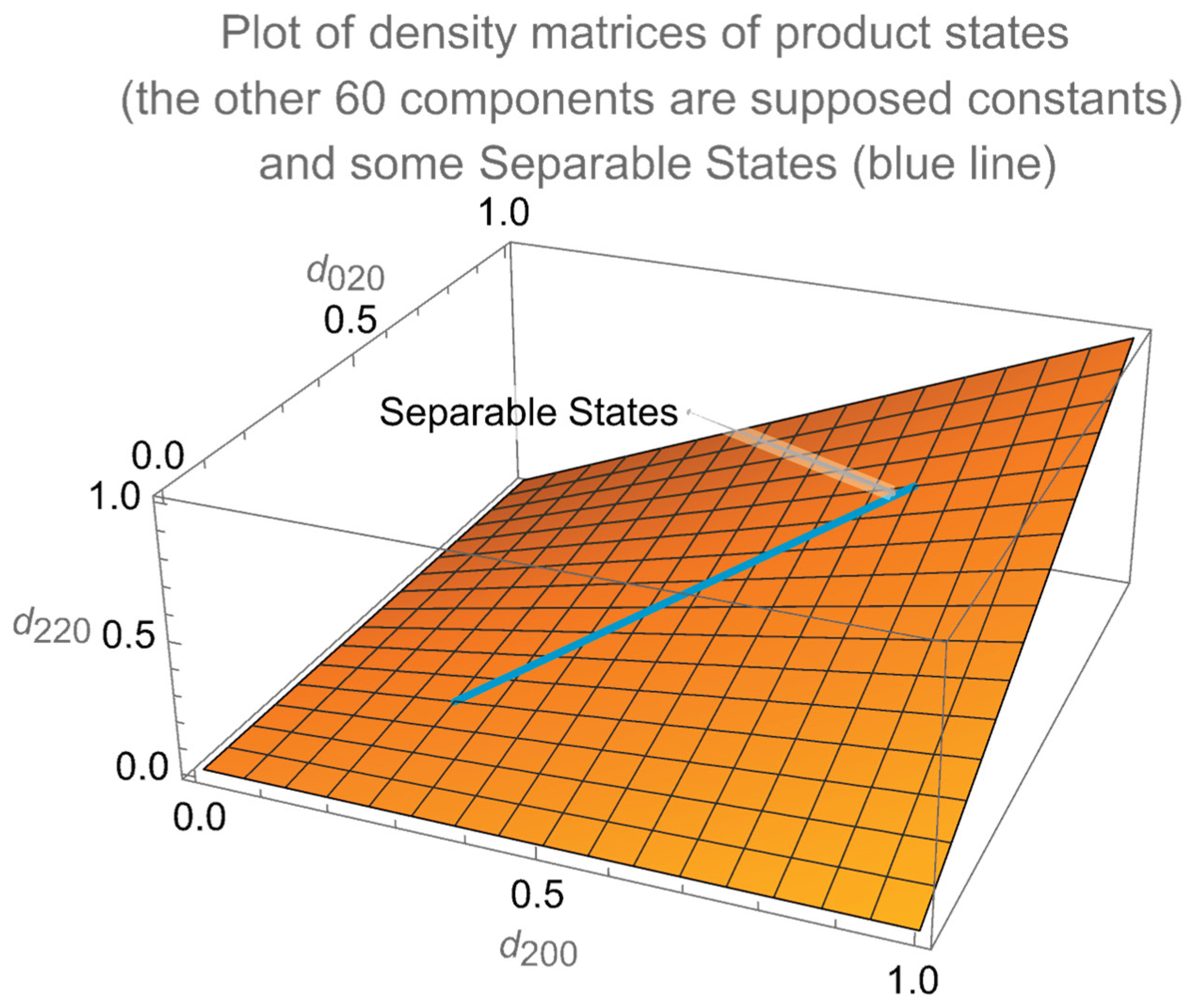
We notice that $L$ is a function from ${\mathbb{R}}^9$ to ${\mathbb{R}}^{63}$. So, we have a 9-dimensional (hyper)surface $T$ embedded in the 63-dimensional manifold ${\mathbb{R}}^{63}$. The (hyper)surface $T$ is the manifold of totally product states into the whole space of tripartite density matrices.

As before if $h$ is the Euclidian metric in ${\mathbb{R}}^{63}$ we can compute the induced metric $g=L^{*}h$. If

$$\begin{gathered} r_1=d_{000}^2+d_{001}^2+d_{002}^2+d_{003}^2 \\ {r}_2=d_{000}^2+d_{010}^2+d_{020}^2+d_{030}^2 \\ {r}_3=d_{000}^2+d_{100}^2+d_{200}^2+d_{300}^2 \end{gathered}$$

(24)

The result is (eq. (4))

$$\begin{gathered} g_{\mu \mu }=r_1{r}_2\mathrm{for}\mu =0,1,2 \\ {g}_{\mu \mu }=r_1{r}_3\mathrm{for}\mu =3,4,5 \\ {g}_{\mu \mu }=r_2{r}_3\mathrm{for}\mu =6,7,8 \\ {g}_{\mu \nu }=r_1{d}_{0,\mu -2,0}{d}_{\nu +1,0,0}\mathrm{for}\mu =3,4,5, \nu =0,1,2 \\ {g}_{\mu \nu }=r_2{d}_{0,0,\mu -5}{d}_{\nu +1,0,0}\mathrm{for}\mu =6,7,8, \nu =0,1,2 \\ {g}_{\mu \nu }=r_3{d}_{0,0,\mu -5}{d}_{0,\nu -2,0}\mathrm{for}\mu =6,7,8, \nu =3,4,5 \\ {g}_{\nu \mu }=g_{\mu \nu } \end{gathered}$$

(25)

The other components of $g$ are 0. We may compute the scalar curvature with “mathematica”, but the expression is too big to be written here.

Figure 2. The function $z=xy$ is plotted to illustrate product states, assuming $x$ and $y$ correspond to elements of the associated density matrices.

Figure 2. The function $z=xy$ is plotted to illustrate product states, assuming $x$ and $y$ correspond to elements of the associated density matrices.

4. Discussion

Differential geometry is a broad and foundational field with wide-ranging applications in physics and other scientific disciplines. The geometrization of product states, along with the computation of associated geometric quantities such as curvature, is expected to offer multiple theoretical and practical advantages. Based on the preceding analysis, the approach can be systematically extended to other systems to identify their corresponding manifolds. Although the required computations may be extensive and technically demanding, this line of inquiry holds significant promise as the foundation for future research.

References

- Schrödinger, E., “Die gegenwärtige Situation in der Quantenmechanik”, Die Naturwissenschaften, 1935, 23, Issue 48, pp.807-812. [CrossRef]
- Einstein, A., Podolsky, B. and Rosen, N., “Can Quantum-Mechanical Description of Physical Reality Be Considered Complete?”, Phys. Rev. 1935, 47, 777. [CrossRef]
- Bennett, C. H. and Wiesner, S. J. “Communication via one- and two-particle operators on Einstein-Podolsky-Rosen states”, Phys. Rev. Lett. 1992, 69, 2881. [CrossRef]
- Bennett, C. H. Brassard, G., Crepeau, C., Jozsa, R., Peres A. and Wootters, W. K. “Teleporting an unknown quantum state via dual classical and Einstein-Podolsky-Rosen channels”, Phys. Rev. Lett. 1993, 70, 1895. [CrossRef]
- Bennett, C. H., DiVincenzo, D. P., Smolin J. A. and Wootters, W.K., “Mixed-state entanglement and quantum error correction”, Phys. Rev. A 1996, 54, 3824. [CrossRef]
- Peres, A., “Separability Criterion for Density Matrices”, Phys. Rev. Lett. 1996, 77, 1413. [CrossRef]
- Horodecki, M., Horodecki, P. and Horodecki, R., “Separability of mixed states: necessary and sufficient conditions”, Phy. Lett. A 1996, 223, 1.
- Fano, U., “Pairs of two-level systems”, Rev. Mod. Phys., 1983, 55:855. [CrossRef]
- Cuncha, M.M., Fonseca, A., Silva, E. O., “Tripartite Entanglement: Foundations and Applications”, Universe 2019, 5(10), 209. [CrossRef]
- Nakahara, M., “Geometry, Topology and Physics”, 2nd ed.; Institute of physics publishing: Bristol and Philadelphia, UK, USA, 2003.
Disclaimer/Publisher’s Note: The statements, opinions and data contained in all publications are solely those of the individual author(s) and contributor(s) and not of MDPI and/or the editor(s). MDPI and/or the editor(s) disclaim responsibility for any injury to people or property resulting from any ideas, methods, instructions or products referred to in the content. |
© 2025 by the authors. Licensee MDPI, Basel, Switzerland. This article is an open access article distributed under the terms and conditions of the Creative Commons Attribution (CC BY) license (http://creativecommons.org/licenses/by/4.0/).
Copyright: This open access article is published under a Creative Commons CC BY 4.0 license, which permit the free download, distribution, and reuse, provided that the author and preprint are cited in any reuse.