
Submitted:
08 September 2025
Posted:
09 September 2025
You are already at the latest version
Abstract
This paper presents a power-centric systems-engineering approach for PlanarSats and for atto-, and femto-class spacecraft where surface-limited power dominates design. We review agency practices (The National Aeronautics and Space Administration (NASA), European Space Agency (ESA), Japan Aerospace Exploration Agency (JAXA)) and the American Institute of Aeronautics and Astronautics (AIAA) framework, then extend them with refined low-power subcategories and a log-linear method for selecting phase- and class-appropriate power contingencies. The method is applied to historical and conceptual PlanarSats to show how contingencies translate into required array area, allowable incidence angles, and duty cycle, linking power sizing to geometry and operations. We formalize the operational power envelope as the range of satellite orientations and conditions for which generated power meets the mission requirement, providing an explicit bridge between requirement-driven and constraint-driven design. We define the operational power envelope as the range of satellite orientations and conditions under which generated power meets or exceeds mission requirements. Consistent with agency guidance, sizing is performed to the maximum expected value (MEV) (CBE plus contingency); when bounding or stress analyses are needed, we report the maximum possible value (MPV) (Maximum Possible Value) by applying justified system-level margins to the MEV. Results indicate that disciplined, phase-aware contingency selection materially reduces power-related risk and supports reliable, scalable PlanarSat missions under severe physical constraints.
Keywords:
PlanarSat
; Attosat
; Femtosat
; Small Satellite
; ChipSat
; Systems Engineering
1. Introduction
Satellite design is fundamentally governed by four constraints: mass, volume, power, and data. Mass is dictated by launch cost, volume by available fairing size, power by the satellite’s ability to generate and store energy, and data by mission objectives. Standardized form factors such as CubeSats and PocketQubes have enabled cost-effective access to space by imposing mass and volume limits; for example, per CubeSat and per PocketQube [1,2].
As the miniaturization of satellites continues, new architectures such as PlanarSats have emerged. PlanarSats are flat satellites with a surface area far larger than their thickness, where the challenge of generating sufficient power on a limited surface becomes dominant. Despite their unique geometry, PlanarSats must provide all core satellite functionalities, though subsystem scaling and layout differ from conventional satellites to fit the planar form factor [3].
A clear, structured approach for PlanarSat system development is not yet available in the literature [3]. As reviewed in [3], the PlanarSat concept is introduced alongside a survey of atto- and femto-satellites, including their dimensions, missions, power, and mass. Kanavouras et al. propose an agile systems engineering methodology for sub-CubeSat spacecraft such as femto- and atto-satellites, enabling rapid development cycles with reduced cost and increased flexibility compared to traditional approaches [4,5]. Ekpo and George introduce a deterministic, multifunctional architecture for highly adaptive small satellites, facilitating reconfigurable designs that yield significant mass and power savings [6,7]. Although these works do not focus specifically on PlanarSats, they provide general, parametric approaches to small satellite design, incorporating “mass” as a key variable based on textbook references [8,9].
The critical challenge for PlanarSats, as for other highly miniaturized platforms, is that as satellites shrink, the available surface area for solar cells decreases rapidly, yet all essential functionalities (processing power, data storage, communication, power systems, payload) must still be included. Literature consistently shows that power budgeting errors are a leading cause of mission failures in small satellites [10,11,12], underscoring the need for a design methodology that prioritizes power from the outset [13,14]. Recent peer-reviewed studies provide detailed examples of power system analysis in current CubeSat missions: Acero et al. (2023) describe a scenario-based approach to electrical power system (EPS) validation, integrating subsystem modeling, operational planning, and margin allocation using real mission data [12]; Kerrouche et al. (2022) document the design and verification of a low-cost CubeSat EPS, including margin practices and lessons from hardware-in-the-loop testing [15]; and Tadanki and Lightsey (2019) present practical subsystem-level power budgets and engineering trade-offs from university-built CubeSats [16]. These studies show how explicit, scenario-driven EPS sizing and contingency selection are applied in practice; an approach we extend to PlanarSats.
One key advantage of PlanarSats is their simple, two-dimensional geometry, which allows direct, empirical analysis of power generation and consumption. Leveraging established guidelines from organizations such as AIAA, NASA, and ESA, it is possible to build a more systematic and robust design process, including the integration of recommended contingencies and margins at every stage of design to ensure mission success.
PlanarSats, by definition, are essentially two-dimensional satellites. Especially at the atto- and femto-satellite levels, they tend to be a single substrate; most often a single printed circuit board (PCB) [3]. Power generation depends on solar cells that directly occupy some of the available surface. Depending on solar-cell technology and efficiency, the required area varies and can limit the surface available for other functions. Conversely, to provide sufficient power, the satellite may need to be sized up to accommodate more solar cells, which in turn increases the area available for other functionalities.
Figure 2 illustrates three foundational PlanarSat configurations based on the allocation of solar cells and electronics: (a) separated; solar cells on one side, electronics on the other; (b) half-mixed; solar cells on one side and a mix of solar cells and electronics on the other; and (c) mixed; both sides carry a combination of solar cells and components. These layouts directly influence power generation, orientation sensitivity, and subsystem integration.
Extreme miniaturization consolidates all essential subsystems;including power, communication, data handling, attitude control, and payload, onto a single substrate (typically a single PCB), with careful allocation of both surface area and power. Figure 1 shows that as satellites shrink, required functionalities remain while available power-generation area diminishes, forcing trade-offs between size, capability, and operational robustness.
Figure 1.
Subsystems and functions for CubeSats (orange), PocketQubes (blue), and PlanarSats (green). Systems are getting smaller, but required functionalities remain the same. Dimensions of the example satellites are given in the bottom right of the respective boxes; in the top right is the approximate footprint of a subsystem for each satellite [17,18,19,20,21,22,23,24,25].
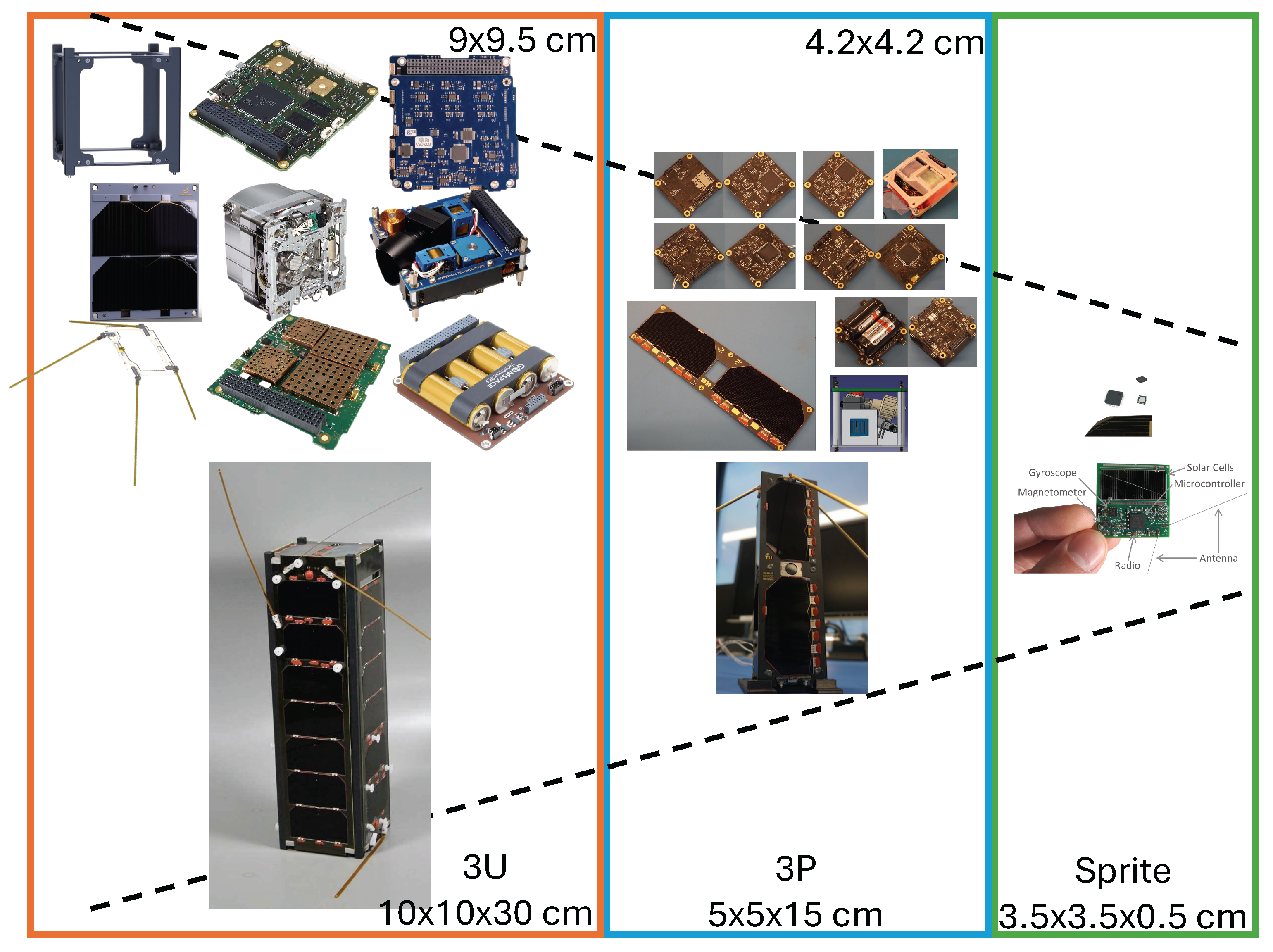
Figure 2.
Basic architecture of PlanarSats. Colors represent: PCB, solar cells, and integrated circuits.Left to right; seperated, half-mixed, and mixed architecture.
Figure 2.
Basic architecture of PlanarSats. Colors represent: PCB, solar cells, and integrated circuits.Left to right; seperated, half-mixed, and mixed architecture.

This study develops a structured, power-driven methodology for atto- and femto-class PlanarSats that adapts NASA/ESA/AIAA contingency/margin philosophy to the surface-constrained regime. The framework supplements—rather than replaces—agency guidance, and is demonstrated on both real and conceptual missions. Key elements include a formal operational power envelope (OPE) to make the reliability implications of power sizing explicit, refined low-power categories with contingency scaling as a transparent extension of existing standards, and a mission-adjusted value that scales the MEV by mission-specific factors (e.g., tumbling incidence, conversion efficiency) to reflect operational uncertainty.
2. Power-Based Satellite Design
The PlanarSat form factor constrains available surface area for both power generation and electronics. A power-centric design process therefore enables a direct, iterative development flow that ties geometry to capability.
In this work, sizing proceeds bottom-up: the process begins from power requirements and surface-area constraints, together with known subsystem needs, and builds the overall design accordingly. For PlanarSats and other ultra-small satellites, limited heritage reduces the reliability of traditional top-down methods common for larger spacecraft. Consequently, this paper derives power subcategories and contingency guidance tailored to these emerging classes.
Contingency factors are considered at each design phase, with iterative updates as maturity increases. To ground the methodology, agency practices from ESA, NASA, and JAXA are summarized in Table 3 (see also Table 1 and Table 2 for definitions and calculation steps). These practices vary with design maturity, product evolution, and risk, and are tracked at key reviews (Preliminary design review (PDR), Critical design review (CDR), Post–shipment review (PSR)). In parallel, AIAA provides phase- and category-dependent guidance for power contingencies (Table 4). Terminology note: agencies differ in nomenclature. For cross-agency comparison in this paper, values in Table 3 are interpreted using the definitions in Table 1: percentages applied to current best estimate (CBE) are treated as contingency (contributing to MEV), while any additional system-level reserves above MEV are treated as margin (defining MPV), when explicitly stated by the source.
2.1. Margin and Contingency: Agency and Textbook Definitions
The terms margin and contingency are central to spacecraft power budgeting but differ in meaning and application across agencies and references. In this paper the following working definitions are used, consistent with agency usage: Contingency is a percentage uplift applied to the CBE to cover known unknowns, estimating uncertainty, and expected growth; Margin is capability retained above MEV to provide robustness and worst-case bounds. Table 1 distills the role of contingency versus margin as used in this paper.
NASA distinguishes contingency (growth allowance) from margin. Contingency is applied to the CBE; CBE+contingency is the MEV. Recommended contingency decreases with maturity (e.g., 30–40% early, 10–20% at PDR, 5–10% at CDR), Table 3. For power systems, NASA recommends sizing to MEV and avoiding additional margin to prevent “pile-up” (Figure 3) [26,27].
ESA often uses margin broadly, encompassing uncertainty allowances and reserves. Typical system-level values start near 20% in early phases and are reduced at CDR (Table 3). ESA guidance explicitly warns against double counting across subsystem and system levels [28].
AIAA specifies both contingency and margin for power systems [29,30]. Contingency is a multiplicative uplift on CBE (e.g., 1.1–1.3 initially, tapering with maturity), applied at the subsystem level and burned down as knowledge grows. A separate system margin (typically 5–20%) is reserved for bounding or stress tests and is not stacked on top of contingency for routine sizing. In most cases, sizing is performed to the MEV; MPV (which includes margin) is used for worst-case bounds.
Space Mission Analysis and Design (SMAD) defines margin as excess capability relative to requirement and contingency as a percentage added to early estimates. Both are emphasized early and reduced with maturity [31]. Elements of Spacecraft Design (ESD) follows a similar process but may report a fraction-of-capability “margin,” which can appear smaller if not clearly defined [9].

Table 1.
Summary of contingency and margin features for system analysis.
| Feature | Contingency | Margin |
|---|---|---|
| Applied to | CBE (estimated demand/cost) | Capability above MEV (demand + contingency) |
| Covers | Known unknowns, estimating error, expected growth | Unknown unknowns, robustness, worst-case bounds |
| Management | Subsystem/team level | Project/program level |
| Trend | Burns down with maturity | Remains positive as design buffer |
Table 2.
Summary of CBE, MEV, and MPV for power system analysis.
| Term | What it Means | How to Calculate | Typical Use |
|---|---|---|---|
| CBE | Best estimate (today’s design) | Engineer’s calculated value | Baseline, preliminary analysis |
| MEV | Maximum expected value (with contingency) | CBE × (1 + contingency %) | Power system sizing |
| MPV | Maximum possible value (with margin) | MEV × (1 + margin %) | Stress/bounding, risk assessment |
Table 2 summarizes the computation pathway (CBE → MEV → MPV) adopted in this work. For sizing in this paper, contingency is applied to each subsystem’s CBE, results are summed to obtain the MEV, and the power system is sized to MEV. Additional system-level margin (MPV) is used only for bounding or explicit mission requirements, avoiding double counting.
Table 3.
Power margins by agency and project phase.
| Agency | Project Phase | Power Margin | Report Timing | Reference(s) |
|---|---|---|---|---|
| ESA | Equipment Level (Off-The-Shelf A/B) | ≥ 5% | During design and development | [32,33,34] |
| ESA | Equipment Level (Off-The-Shelf C) | ≥ 10% | During design and development | [32,33,34] |
| ESA | Equipment Level (New Design/Major Modification D) | ≥ 20% | During design and development | [32,33,34] |
| ESA | System Level (General) | ≥ 20% of nominal power | Throughout project lifecycle | [32,34] |
| ESA | System Level (IOD CubeSat at PDR) | 20% | At Preliminary Design Review (PDR) | [32,34] |
| ESA | Pre-PDR | 20% | Before Preliminary Design Review (PDR) | [32,34] |
| ESA | Pre-CDR | 10% | Before Critical Design Review (CDR) | [32,34] |
| ESA | At PDR | 5–15% | Preliminary Design Review (PDR) | [32,34,35] |
| ESA | At CDR | 5–15% | Critical Design Review (CDR) | [32,34,35] |
| NASA | Phase B (Formulation) | ∼30% | During Preliminary Design Phase | [36,37,38] |
| NASA | Initial Design (SMAD Recommendation) | 25% | Initial design phase | [36,38] |
| NASA | Historical Average (Aerospace Corporation Study) | ∼40% | Throughout design phases | [36,37,38,39] |
| NASA | At PDR | 20% | Preliminary Design Review (PDR) | [36,37,38] |
| NASA | At CDR | 10% | Critical Design Review (CDR) | [36,38] |
| JAXA | PDR (New bus & payload) | 15% | At Preliminary Design Review (PDR) | [38,40,41] |
| JAXA | CDR (New bus & payload) | 10% | At Critical Design Review (CDR) | [38,40,41] |
| JAXA | PSR (New bus & payload) | 6% | At Post-Shipment Review (PSR) | [38,40,41] |
| JAXA | PDR (Large changes to existing bus/payload) | 10% | At Preliminary Design Review (PDR) | [38,40,41] |
| JAXA | CDR (Large changes to existing bus/payload) | 8% | At Critical Design Review (CDR) | [38,40,41] |
| JAXA | PSR (Large changes to existing bus/payload) | 6% | At Post-Shipment Review (PSR) | [38,40,41] |
| JAXA | PDR (Minor changes to existing bus/payload) | 5% | At Preliminary Design Review (PDR) | [38,40,41] |
| JAXA | CDR (Minor changes to existing bus/payload) | 8% | At Critical Design Review (CDR) | [38,40,41] |
| JAXA | PSR (Minor changes to existing bus/payload) | 4% | At Post-Shipment Review (PSR) | [38,40,41] |
| JAXA | PDR (Existing bus & payload) | 5% | At Preliminary Design Review (PDR) | [38,40,41] |
| JAXA | CDR (Existing bus & payload) | 5% | At Critical Design Review (CDR) | [38,40,41] |
| JAXA | PSR (Existing bus & payload) | 3% | At Post-Shipment Review (PSR) | [38,40,41] |
The AIAA power categories provide a structured basis for scaling contingencies with mission class and power level (Table 4). This scaling is particularly relevant for small satellites, where limited generation area, conversion losses, and reduced redundancy increase risk. In contrast, broader agency values (e.g., a uniform 20% system-level margin) may not capture low-power sensitivities. For this reason, the AIAA framework is used as a starting point, then extended to the very low power regime.
Table 4.
AIAA recommended minimum standard power contingencies in %. Category descriptions follow [9,30,42].
| Proposal Stage | Design Development Stage | ||||||||||||||
| Bid Class |
CoDR Class |
PDR Class |
CDR Class |
PRR Class |
|||||||||||
| Description/ Categories |
1 | 2 | 3 | 1 | 2 | 3 | 1 | 2 | 3 | 1 | 2 | 3 | 1 | 2 | 3 |
| Category AP 0-500 W |
90 | 40 | 13 | 75 | 25 | 12 | 45 | 20 | 9 | 20 | 15 | 7 | 5 | 5 | 5 |
| Category BP 500-1500 W |
80 | 35 | 13 | 65 | 22 | 12 | 40 | 15 | 9 | 15 | 10 | 7 | 5 | 5 | 5 |
| Category CP 1500-5000 W |
70 | 30 | 13 | 60 | 20 | 12 | 30 | 15 | 9 | 15 | 10 | 7 | 5 | 5 | 5 |
| Category DP 5000 W and up |
40 | 25 | 13 | 35 | 20 | 11 | 20 | 15 | 9 | 10 | 7 | 7 | 5 | 5 | 5 |
However, the lowest existing bin (0–500 W) is too coarse for nano/pico/femto/atto systems. Refined subcategories and associated contingencies are therefore defined as follows.
2.2. Definition of Power Subcategories
The lowest established AIAA bin is 0–500 W (Table 4) [9,30]. PlanarSats operate far below this level, motivating a more granular breakdown. Notional upper bounds for standardized classes (CubeSats, PocketQubes) are estimated using a representative commercial solar cell (4×8 cm, ∼30% efficiency, 1.2 W at normal incidence) [43]. Cells are mounted on each face, and for comparability across classes a three-face, 45° illumination convention is assumed. This is a normalization scenario for category derivation; actual duty cycles and attitudes are handled in mission analysis. The three-face, 45° convention is not a physically realizable solar geometry and is used solely to derive power bins on a consistent basis across form factors; mission- and attitude-dependent power is treated later through the standard budget and contingency process.
where is the BoL normal-incidence array power at AM0 and captures conversion/wiring efficiencies. For free-tumbling PlanarSats, a mission-averaged consistent with expected attitude dynamics is used in later analyses.
Table 5.
Standardized small satellites equipped with the maximum number of standard solar cells [43] on X, Y, and Z faces. Power is computed for a 45° incidence on three faces.
Table 5.
Standardized small satellites equipped with the maximum number of standard solar cells [43] on X, Y, and Z faces. Power is computed for a 45° incidence on three faces.
| Number of Cells on Surfaces |
Maximum Power at 45 degrees |
|||
| X | Y | Z | Total [W] | |
| 16U | 20 | 20 | 8 | 40.73 |
| 12U | 14 | 14 | 8 | 30.55 |
| 8U | 20 | 10 | 4 | 28.85 |
| 6U | 14 | 7 | 4 | 21.21 |
| 4U | 10 | 10 | 2 | 18.67 |
| 3U | 7 | 7 | 2 | 13.58 |
| 2U | 4 | 4 | 2 | 8.49 |
| 1U | 2 | 2 | 2 | 5.09 |
| 3P | 2 | 2 | 0.5 | 3.82 |
| 2P | 1.5 | 1.5 | 0.5 | 2.97 |
| 1.5P | 1 | 1 | 0.5 | 2.12 |
| 1P | 0.5 | 0.5 | 0.5 | 1.27 |
| 0.5P | 0.25 | 0.25 | 0.5 | 0.85 |
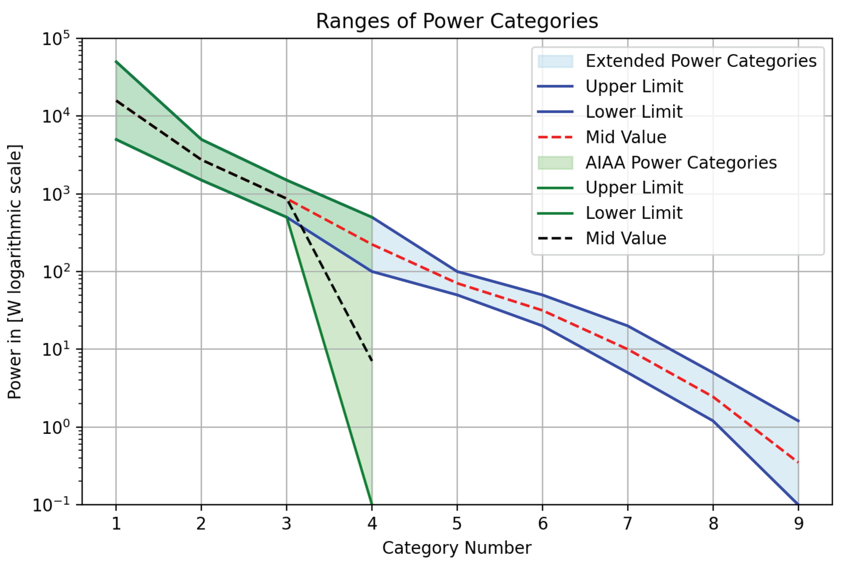
Analysis of the resulting levels shows that conventional bins are too coarse. A four-level breakdown (50–20 W, 20–5 W, 5–1.2 W, 1.2–0 W) aligns with achievable power trends and supports downstream estimation. Combining original and extended bins yields: 5000+ W, 5000–1500 W, 1500–500 W, 500–100 W, 100–50 W, 50–20 W, 20–5 W, 5–1.2 W, and 1.2–0 W. The 100–50 W bin bridges the gap between legacy AIAA categories and the new low-power bins.
Figure 4.
Power level categories: original AIAA (green) [30], extended bins (blue), and geometric means (black/red dashed) used for extrapolation. Lower bound is 0.1 W (log scale).
Figure 4.
Power level categories: original AIAA (green) [30], extended bins (blue), and geometric means (black/red dashed) used for extrapolation. Lower bound is 0.1 W (log scale).
2.3. Investigation of Contingencies for Lower Power Categories
Because historical data are sparse at very low power, contingency values below 500 W are extrapolated from higher-power anchors in Table 4. Alternatives were assessed (linear, spline, piecewise). Linear methods can mislead over wide dynamic ranges [46]; higher-order fits can oscillate with sparse data [47]. Given the multi-decade span and near-exponential behavior, log-linear interpolation is adopted as a conservative, consistent choice.
Each bin is represented by the geometric mean of its endpoints. For the lowest bin (0–1.2 W), a 0.1 W lower bound avoids . The extrapolated contingency at is computed as
where and are adjacent known anchors. Extrapolated values are calculated in log space, then rounded to the nearest 5%; values exactly halfway between multiples of 5 are rounded to the higher multiple. Anchor values are retained as published.
Applying this to AIAA anchors yields the extended recommendations in Table 6. The main text reports rounded values for engineering clarity; unrounded values appear in Table A1 (Appendix). This provides a transparent, repeatable extension into regimes with limited heritage.
At the lowest powers and earliest phases, some Class I values exceed 100% (e.g., Bid at 0–1.2 W). This is consistent with agency practice permitting high early-phase contingencies for first-of-kind or tightly constrained designs [28,48,49]. Such values reduce with maturity (PDR/CDR), as reflected in Table 6.
2.4. Sensitivity Analysis for Extrapolated Contingency Values
All sub-500 W recommendations are produced by stepwise, log-linear extrapolation from higher-power anchors (Table 4), evaluated at each bin’s geometric center via Eq. 2. Extrapolated values are then rounded to the nearest 5 percentage points, and the rounded value is propagated as the next anchor; values exactly halfway between multiples of 5 are rounded to the higher multiple. Published anchors from AIAA are retained as given. For the lowest bin (0–1.2 W), a lower bound of 0.1 W is used to avoid .
Sensitivity is assessed with two one-at-a-time sweeps for PDR, Class II:
- Sweep A (left block): Vary the 500–1500 W anchor (5, 10, 15, 20%) with 100–500 W fixed at 20%.
- Sweep B (right block): Vary the 100–500 W anchor (15, 20, 25, 30, 35%) with 500–1500 W fixed at 15%.
Table 7.
Sensitivity of stepwise log-linear extrapolation (PDR, Class II). Each entry shows the unrounded value followed by the rounded value in parentheses. Extrapolated values are rounded to the nearest 5 percentage points at each step; the rounded value is used as the next anchor. Underlined values in the header row shows the baseline/actual values.
| Sweep A: 500–1500 W anchor (%), 100–500 W = 20% | 15 | 20 | 25 | 30 | 35 | ||||
| Power Bin (W) | 5 | 10 | 15 | 20 | Sweep B: 100–500 W anchor (%), 500–1500 W = 15% | ||||
| 50–100 | 32.75 (35) | 28.50 (30) | 24.25 (25) | 20.00 (20) | 15.00 (15) | 24.25 (25) | 33.50 (35) | 42.75 (45) | 52.01 (50) |
| 20–50 | 45.48 (45) | 36.99 (35) | 28.49 (30) | 20.00 (20) | 15.00 (15) | 28.49 (30) | 41.99 (40) | 55.48 (55) | 60.48 (60) |
| 5–20 | 59.31 (60) | 42.15 (40) | 37.15 (35) | 20.00 (20) | 15.00 (15) | 37.15 (35) | 47.15 (45) | 69.31 (70) | 74.31 (75) |
| 1.2–5 | 78.33 (80) | 46.11 (45) | 41.11 (40) | 20.00 (20) | 15.00 (15) | 41.11 (40) | 51.11 (50) | 88.33 (90) | 93.33 (95) |
| 0–1.2 | 107.81 (110) | 51.95 (50) | 46.95 (45) | 20.00 (20) | 15.00 (15) | 46.95 (45) | 56.95 (55) | 117.81 (120) | 122.81 (125) |
Rounding policy: per-step versus end-of-cascade.
This work adopts per-step rounding because it reflects baselined values carried between design reviews (e.g., PDR, CDR), avoids false precision, and provides appropriate conservatism when heritage is sparse. End-of-cascade values are shown for diagnostic comparison only; per-step rounding is used in this work for all subsequent sizing. The table below compares per-step and end-of-cascade rounding for two cases, reporting unrounded (rounded) values so the computed quantities are visible:
- Baseline: 500–1500 W = 15%, 100–500 W = 20%.
- High-gradient: 500–1500 W = 15%, 100–500 W = 30%.
Table 8.
Comparison of rounding policies (PDR, Class II), showing unrounded (rounded).
| Power Bin (W) | Baseline: Per step | Baseline: End of cascade | High-gradient: Per step | High-gradient: End of cascade |
|---|---|---|---|---|
| 50–100 | 24.25 (25) | 24.25 (25) | 42.75 (45) | 42.75 (45) |
| 20–50 | 28.49 (30) | 27.22 (25) | 55.48 (55) | 51.67 (50) |
| 5–20 | 37.15 (35) | 31.47 (30) | 69.31 (70) | 64.42 (65) |
| 1.2–5 | 41.11 (40) | 36.67 (35) | 88.33 (90) | 80.01 (80) |
| 0–1.2 | 46.95 (45) | 43.89 (45) | 117.81 (120) | 101.68 (100) |
Lower-bound check for the 0–1.2 W bin.
Using a 0.2 W lower bound (instead of 0.1 W) yields 45.72% (unrounded) versus 46.95% (unrounded) in the baseline; both round to 45%. Thus the reported rounded value is insensitive to the exact lower-bound choice in this range.
In summary, anchor spacing (the difference between consecutive higher-power anchors) is the dominant driver of low-power results. With the adopted per-step rounding, the cascade is stable, conservative, and aligned with baselining practice at PDR/CDR; deferring rounding to the end reduces some intermediate bins by approximately 5 pp and can materially lower extreme early-phase values (e.g., 120% → 100%) in high-gradient cases.
3. Case Study: Application to Real/Conceptual Satellites
To demonstrate the value and practical application of the proposed contingency and power-margin methodology, several representative PlanarSat missions are analyzed in the femto- and atto-satellite classes. The missions—Sprite V1, Sprite V2, PCBSat, SpaceChip, and LuxAtto—span a range of technical choices, design phases, and power budgets, providing a comprehensive view of the methodology’s applicability and its impact on design trade-offs. Figure 5 presents the mission set; Figure 6 later provides a project-level illustration using sequential Sprite variants.
- Mission set and phase/class assignment.
Five missions are considered and summarized in Table 9:
3.1. Case-by-Case Insights and Methodological Lessons
Unless otherwise noted, instantaneous power is single-sided, meaning only the Sun-facing face produces power at a given moment. Dual-sided coverage improves orbit-average yield under tumbling, but it does not imply simultaneous two-sided illumination.
PCBSat and SpaceChip. PCBSat’s as-built generation (up to 1131 mW at normal incidence) exceeded its CBE but was below the recommended MEV of 1529.3 mW for Class I at conceptual design review (CoDR). The original design used a 45° sizing angle and included conversion losses [51]. At that level, CBE is met only when incidence is roughly 45° or better; larger angles or longer eclipses reduce margin. Sizing to MEV would increase tolerance to degraded pointing and tumbling, with a required PCB-side area increase of 47.13% (equivalently, a required solar area of ∼96.30 cm2 at normal incidence). For a planar architecture, that growth maps directly to PCB planform, which may influence board mass, stiffness, and rideshare accommodation.
SpaceChip used very low efficiency cells (about 1%) and no attitude determination and control system (ADCS). The reported normal-incidence capability is 1.87 mW, with a 45° sized value of 1.34 mW. The MEV of 2.51 mW at Bid (Class I) implies a 19.5% PCB area increase (Req. Solar Area (MEV) ∼3.06 cm2 at normal incidence). Although small in absolute terms, even modest planform changes at this scale compete with component footprints and interconnect routing. Sizing to MEV expands the usable attitude envelope without major integration penalties.
LuxAtto (Primary and A&B). For LuxAtto P, the available generation of 105.2 mW at normal incidence is below the CBE of 462 mW, so operations rely on battery energy [53]. Sizing to the MEV of 669.9 mW (Class II at PDR) raises incidence tolerance at a given duty cycle and enables faster recharge. This requires a 316.00% increase in PCB side area, from 12.5 cm2 to 52 cm2 in the documented envelope (equivalently, a required solar area of ∼46.85 cm2 at normal incidence). Because solar area scales the PCB planform for PlanarSats, this growth has programmatic implications: larger panel outlines tend to increase manufacturing cost and handling complexity, reduce panel yield per panelization sheet, lengthen harness runs, and raise assembly risk; dispensers or rideshare slots sized for a given footprint may accommodate fewer units, or a larger envelope may need to be purchased; higher exposed area can alter thermal radiation balance, increase solar-radiation-pressure and aerodynamic torques, and modestly increase drag, which can shorten lifetime in low orbit unless compensated elsewhere.
For LuxAtto A&B, the CBE is 70 mW with 52.6 mW generation at normal incidence. Sizing to the MEV of 119 mW (Class I at PDR) reduces time in power deficit. The required PCB side area increase is 54.72%, from 6.25 cm2 to 9.67 cm2, which is significant for multi-unit deployments. Practical effects include tighter packing in dispensers or trays, reduced unit count for a fixed envelope, higher per-unit board cost due to lower panelization efficiency, and potential updates to structure and thermal interfaces.
Sprite V1 and V2. Sprite V1’s CBE of 126 mW slightly exceeds its per-side normal-incidence maximum of 123 mW. Consequently, continuous full-CBE operation under single-sided illumination is not achievable without intermittent duty cycling or storage; near normal incidence, however, reduced-duty operation remains feasible with low losses [56]. With limited storage, performance falls with larger incidence angles, for example when the radio draws 60 mW. Sizing to the MEV of 182.7 mW (Class I at CDR) increases operational robustness under tumbling. The minimum board-area growth cited for this case is 18.12%, from 12.25 cm2 to 14.47 cm2. Even small absolute increases at this scale matter, because they reduce edge clearance for antennas, affect stiffness and modal behavior, and can change radiator view factors.
Sprite V2 benefits from heritage (Class II at CDR) and has a lower MEV of 159.6 mW. Per-side normal-incidence generation is 68 mW; dual-sided coverage improves orbit-average yield during tumbling but does not change the single-sided instantaneous limit. Meeting the MEV requires a 28.57% increase in board area, from 12.25 cm2 to 15.74 cm2. Similar to V1, planform growth at this scale has practical impacts on component placement, connector reach, and structural margins.
Table 10.
Summary of key power metrics for analyzed satellites. Assumed project phases and classes are shown. As-built Solar Area is as flown or as documented; Req. Solar Area (MEV) is the normal-incidence area needed to meet MEV; PCB-side Area Inc. is the increase in single-side PCB planform adopted in the case studies to achieve MEV.
| As-built | Req. Solar | PCB | Notes | |||||
| Satellite | Class | Phase | Contingency | MEV | Solar Area | Area (MEV) | Area Inc. | |
| (%) | (mW) | (cm2) | (cm2) | (%) | ||||
| SpaceChip | I | Bid | 120 | 2.51 | 2.28 | 3.06 | 19.5 | Concept, 1% cell |
| PCBSat | I | CoDR | 105 | 1529.3 | 56.00 | 96.30 | 47.13 | Concept/Prototype |
| LuxAtto A&B | I | PDR | 70 | 119.0 | 3.68 | 8.32 | 54.72 | New form factor |
| LuxAtto P | II | PDR | 45 | 669.9 | 7.36 | 46.85 | 316.00 | Predecessor: Sprite |
| Sprite V1 | I | CDR | 45 | 182.7 | 4.55 | 6.77 | 18.12 | First of kind |
| Sprite V2 | II | CDR | 40 | 159.6 | 2.60 | 6.10 | 28.57 | Heritage from V1 |
Method: Req. Solar Area (MEV) is computed as Areq = MEV/ρP using the power densities in Table 9. For SpaceChip, ρP is estimated from the reported normal-incidence capability (1.87 mW) and solar area (2.28 cm2), giving ρP ≈ 0.82 mW cm−2. If sizing at a worst-case incidence θ (e.g., 45°), multiply Areq by 1/ cos θ.
3.2. From MEV to MPV: Adding Operational and Heritage Margins
The case studies above use MEV as the sizing target, which avoids contingency pile-up. MPV remains useful for bounding analyses or where program rules require additional reserves. Two effects are particularly relevant at ultra-low power:
- Operational effect: Free tumbling or limited ADCS reduces average effective incidence; designs sometimes specify a worst-case incidence for sizing rather than relying on normal-incidence capability.
- Heritage effect: When a later-phase design has a lower MEV than an earlier phase but retains the earlier, larger array, the difference functions as de facto margin at the later phase.
Example: project-level illustration with the Sprite family.
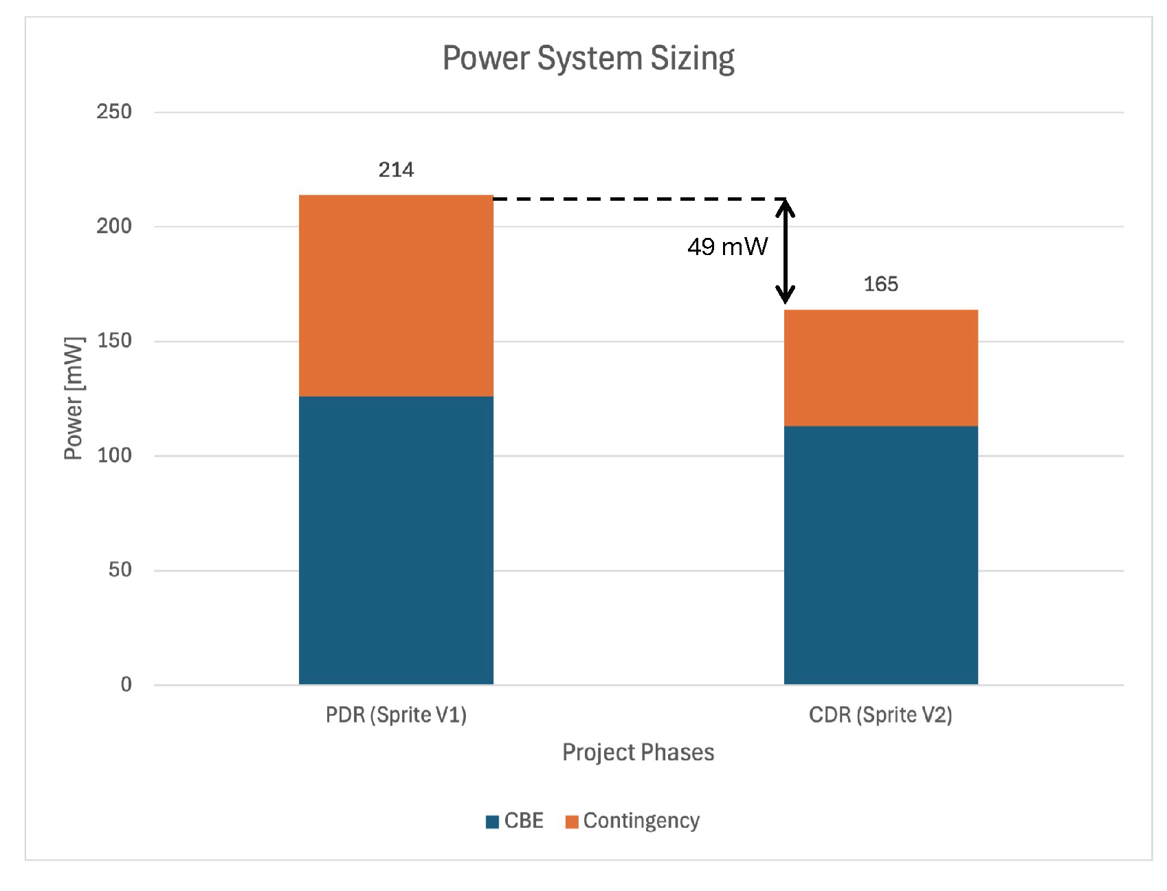
At PDR, Sprite V1 has CBE = 123 mW with 70% contingency, giving MEV = 214 mW. At CDR for Sprite V2, CBE = 114 mW with 45% contingency, giving MEV = 165 mW. Retaining the earlier sizing yields a heritage-derived buffer of mW, so
Figure 6.
Project-level illustration using sequential Sprite variants: MEV reduction from PDR (Sprite V1) to CDR (Sprite V2). Retaining earlier sizing yields a heritage-derived buffer contributing to MPV.
Figure 6.
Project-level illustration using sequential Sprite variants: MEV reduction from PDR (Sprite V1) to CDR (Sprite V2). Retaining earlier sizing yields a heritage-derived buffer contributing to MPV.
Design feasibility check.
Physical limits such as maximum available solar area, PCB outline, dispenser geometry, and budget place a ceiling on achievable MPV. If a computed MPV exceeds feasible capability, MPV should be reset to the realizable bound so that risk and expectations remain aligned with deliverable hardware.
Overall, the consolidated results reinforce three points. First, class- and phase-appropriate contingencies provide a consistent, review-ready basis for PlanarSat power sizing. Second, instantaneous generation is single-sided, so dual-sided coverage helps only the orbit-average under tumbling. Third, making orientation assumptions explicit and recognizing that solar area directly drives PCB planform helps avoid optimistic claims and ties power sizing to real integration, cost, and rideshare constraints.
4. PlanarSat System Development Approach
While the example in this section uses ideal solar cell performance values (for example, Sun angle, AM0 irradiance, no degradation), this is for demonstration clarity. In real missions, power generation capability should be scaled using mission-specific factors such as incidence-angle statistics and conversion efficiency, as discussed earlier. Applying these factors to the MEV yields an MPV that reflects a more realistic power design target under operational uncertainties.
Most PlanarSats in the femto and atto ranges do not include a battery. The reasons include direct temperature exposure, cost (financial and protection-circuit development time), and especially limited volume. Given the single-plane structure and the possibility of using both surfaces, three initial configurations are commonly considered. Depending on resources and mission criticality, designers may select among:
As introduced in Figure 2 (see Section 1), these options establish the foundational trade-offs for PlanarSat system design.
In the absence of active attitude control, PlanarSats are typically modeled as free tumblers. Actual attitude statistics depend on geometry, mass distribution, orbit, and environment, and may show some weak preferential orientations. For the comparative analyses here, we assume single-sided instantaneous power; only the Sun-facing side generates at a given moment. Two-sided coverage improves orbit-average energy under tumbling, but it does not imply simultaneous two-sided illumination. Performance can be improved with ADCS (for example, magnetorquers for Sun pointing), although the ADCS power must be included in the budget.
4.1. A PlanarSat Design: Operational Power Envelopes
The design of current femto and atto PlanarSats is rooted in practical experience and available components [3], with detailed examples in [51,52] based on SMAD [31]. Limited flight heritage at these scales leads to higher design uncertainty. This subsection shows how phase- and class-appropriate contingency and margin can inform sizing and operational analysis using a realistic example.
We consider a single-sided (separated) concept to illustrate the path from CBE to MEV to MPV, and the reverse (constraint-driven) viewpoint. Representative components are: MCU (STM32L496RGT6, , at ) [60], transceiver (SX1278IMLTRT, , during transmit at , receive) [61], and a generic payload (, including peripherals). The satellite operates in two primary modes: transmission (MCU + transmitter) and payload with receiver active; receive is assumed active except during transmission. The CBE for transmission is , which places the design in the 0– category of Table 6. As a first-of-kind mission (Class I) at Bid, a contingency is applied. For illustration only, a system margin is then added to form MPV.
Table 11.
Representative component areas and references (payload entry is illustrative).
| Component | Area [cm2] | Reference |
| STM32L496RGT6 MCU | 1.96 | [60] |
| SX1278IMLTRT Transceiver | 0.49 | [61] |
| Example payload (illustrative) | 2.00 |
We use the planar cosine relation defined earlier (Eq. 1) to interpret operational envelopes versus incidence angle. As shown in Figure 7, the maximum allowable for full operation is set by the ratio of available array power to required power (MEV or MPV). Lower provides surplus power that can be used for additional functions or robustness.
SubFigure 7b–d show the operational envelopes for the three architectures (as defined in Figure 2) when arrays are sized to MEV. In the separated case (b), generation occurs only when the solar face is Sun-facing. In the mixed case (c), placing cells on both faces allows operation in either orientation at the expense of added cell count and cost. The half-mixed design (d) places a full array on one face and a smaller area on the reverse, resulting in different allowable incidence angles depending on which face is Sun-facing. SubFigure 7e–g repeat the analysis for MPV sizing, showing the expected expansion of operational envelope. The figure assumes single-axis variation in incidence for clarity; mission-specific attitude statistics should be used when available.
Over-allocating margin can increase cost, complexity, and mass without proportional risk reduction. In line with NASA’s concurrent engineering resource management guidance [26], margin and contingency should be applied judiciously and refined as the design matures.
Sizing Example: Requirement-Driven vs. Constraint-Driven for a Separated PlanarSat
We present a worked example using typical component footprints and AM0 solar-cell performance. Unless noted, we adopt the AZUR Space 3G30A beginning-of-life normal-incidence power density of at AM0 [43]. The total electronics footprint is
These values are beginning-of-life and exclude incidence, temperature, wiring, and conversion derates, which are captured in the mission-specific MPV factor.
(1) Requirement-driven sizing (power first).
With CBE and contingency, MEV . Adding system margin gives MPV . Required solar areas at normal incidence are
For a separated layout, the board side length is set by the larger of the solar face and the electronics face:
(2) Constraint-driven sizing (fixed outline first).
If the outline is fixed by manufacturing or rideshare constraints, the available solar area on the solar face equals the full face area for a separated architecture. For a compact board,
This falls short of the MEV target of even at normal incidence, so geometry alone forces a power deficit that will grow with off-nominal incidence or conversion losses. For a larger outline,
Table 12.
Separated configuration sizing: requirement-driven and constraint-driven cases at normal incidence.
Table 12.
Separated configuration sizing: requirement-driven and constraint-driven cases at normal incidence.
| Approach | Surface Area (cm2) | Side Length (cm) | Power Target or Max (mW) |
|---|---|---|---|
| Constraint-driven (fixed cm) | 6.25 | 2.50 | 248.5 (max) |
| Requirement-driven (MEV) | 6.96 | 2.64 | 276.54 |
| Requirement-driven (MPV) | 8.35 | 2.89 | 331.85 |
| Constraint-driven (fixed cm) | 25.00 | 5.00 | 994 (max) |
This example shows the direct, quantitative link between surface allocation, power-margin methodology, and hardware feasibility. Actual operational power will be reduced by incidence, temperature, wiring, and conversion losses, which should be captured in mission-specific MPV factors and verified with attitude statistics.
This approach provides a basis for subsequent steps such as explicit surface allocation among subsystems and optimization of power–data trades under strict geometric constraints. While the examples here demonstrate the core architectural effects, a full comparison among designs with detailed allocation and phase-based contingency is left for future work.
Finally, the present work does not include validation through flight data or end-to-end simulations. The use of MEV and MPV follows established power-aware sizing practice, but the framework should be validated against mission-specific dynamics such as tumbling, degradation, and off-nominal incidence. Agency standards remain a solid baseline; however, at extreme miniaturization levels a tailored, geometry- and context-specific application is required. Future efforts will focus on validating and refining the framework through higher-fidelity analyses and mission demonstrations.
4.2. Applicability and Limitations at the Atto Scale
Here, “atto-class” refers to spacecraft with wet mass below . The contingency–margin framework (CBE→MEV→MPV), the rounding policy, and the operational power envelope construction with single-sided instantaneous generation and separated/half-mixed/mixed layouts are scale neutral and apply at this mass range.
Quantitative inputs, however, must be calibrated for designs. In practice this means measuring, for the chosen implementation: (i) photovoltaic performance and interconnect losses on very small panels, (ii) conversion and distribution efficiency and start-up thresholds at W–mW loads, and (iii) attitude and environment effects for low-inertia bodies that inform mission-specific MPV derates. With these inputs measured, the framework applies unchanged. Until such data are available for a given implementation, atto-class numbers should be treated as preliminary and updated as characterization results become available.
5. Conclusion and Future Work
This work introduced a structured, power-based systems engineering methodology for PlanarSats and, more broadly, atto-, femto-, and pico-class satellites. By extending contingency and margin philosophies from NASA, ESA, JAXA, and AIAA to the ultra-low-power regime, we provided a scalable framework for sizing and verifying power systems where available surface area is the dominant constraint.
Detailed low-power subcategories and a log-linear extrapolation of AIAA anchor values were developed to populate contingency guidance below 500 W (Table 6). A sensitivity study (Section 2.4) showed that extrapolated values are driven primarily by the gradient between adjacent anchors, and that rounding to the nearest 5% at each step yields stable, monotonic, and transparent recommendations suitable for engineering use. The consolidated definitions of contingency and margin, aligned with agency practice, separate uncertainty allowances applied to the current best estimate (CBE) from system-level buffers, and avoid double counting by sizing to MEV for routine design while reserving MPV for bounding analyses.
We linked this margin philosophy to hardware geometry through the operational power envelope concept (Figure 7). The envelope quantifies the set of orientations and environmental states in which available power meets or exceeds demand, making the reliability implications of power sizing explicit for separated, half-mixed, and mixed PlanarSat layouts (Figure 2 and Figure 7). A worked example demonstrated requirement-driven and constraint-driven sizing for a separated configuration, with single-sided instantaneous generation stated explicitly. This clarified that two-sided cell coverage improves orbit-average yield under tumbling but does not imply simultaneous illumination, a frequent source of over-optimistic power claims in miniaturized designs.
Application to historical and conceptual missions (Sprite V1/V2, PCBSat, SpaceChip, LuxAtto) showed how class and phase reduce contingency as design maturity and heritage increase, and how MEV-based sizing translates directly into surface area, mass, and cost implications (Section 3.1 and Table 10). For low-power PlanarSats that operate near the edge of feasibility, the methodology makes these trade-offs quantitative and reviewable, helping to reduce the risk of under-designed power systems, a recurring root cause of small-satellite shortfalls.
Future work will expand the empirical basis for atto- and femto-class systems, refine subcategory contingencies as flight data and ground testing accumulate, and integrate additional system constraints into the power and surface allocation process. Priorities include: (i) incorporating temperature, degradation, wiring, and conversion losses into mission-specific MPV factors tied to attitude statistics; (ii) co-optimization of solar array placement with payload, communications, and thermal design; and (iii) higher-fidelity analyses or hardware-in-the-loop demonstrations to validate the operational power envelope under tumbling and partial illumination. As datasets grow, the tables and envelopes presented here can be recalibrated and extended, providing a living, scale-aware methodology for robust PlanarSat power system design.
Author Contributions
Conceptualization, M.S.U.; methodology, M.S.U.; software, M.S.U.; validation, M.S.U. and A.R.A.; formal analysis, M.S.U.; investigation, M.S.U.; resources, M.S.U.; data curation,M.S.U.; writing—original draft preparation, M.S.U.; writing—review and editing, M.S.U. and A.R.A.; visualization, M.S.U.; supervision, A.R.A.; project administration, M.S.U.; funding acquisition, M.S.U. and A.R.A. All authors have read and agreed to the published version of the manuscript.
Funding
This research received no external funding.
Institutional Review Board Statement
Not applicable.
Informed Consent Statement
Not applicable.
Data Availability Statement
The original contributions presented in the study are included in the article, further inquiries can be directed to the corresponding author.
Acknowledgments
The authors thank Assistant Prof. Onur Çelik, Assistant Prof. Stefano Speretta and Dr. Erdem Turan for their feedback, comments and support.
Conflicts of Interest
The authors declare no conflicts of interest.
Abbreviations
The following abbreviations are used in this manuscript:
| ADCS | attitude determination and control system |
| AIAA | American Institute of Aeronautics and Astronautics |
| Bid | bidding |
| BoL | beginning of life |
| BOM | bill of materials |
| CBE | current best estimate |
| CDR | critical design review |
| CoDR | conceptual design review |
| COTS | commercial off-the-shelf |
| DOD | Department of Defence |
| ESA | European Space Agency |
| ESD | Elements of Spacecraft Design |
| EPS | electrical power system |
| FRR | flight readiness review |
| IC | integrated circuit |
| ISS | International Space Station |
| JAXA | Japan Aerospace Exploration Agency |
| MCU | microcontroller |
| MDPI | Multidisciplinary Digital Publishing Institute |
| MEV | maximum expected value |
| MPV | maximum possible value |
| NASA | National Aeronautics and Space Administration |
| OPE | operational power envelope |
| PCB | printed circuit board |
| PDR | preliminary design review |
| PRR | pre–ship readiness review |
| PSR | post–shipment review |
| SMAD | Space Mission Analysis and Design |
Appendix A
Table A1.
Extended Recommended Power Contingencies based on AIAA contingencies (minimum standard power reserve percentages) [30]. Original anchor values are maintained; extrapolated values are shown in italic. “Bid” corresponds to Proposal phase bid estimates; CoDR to Concept Design Review; PDR to Preliminary Design Review; CDR to Critical Design Review; and PRR to Production/Flight Readiness Review. Mission Class I refers to a completely new spacecraft (unique and first-generation); Class II represents the next generation of spacecraft that builds upon a previously established design, offering increased complexity or capability within the same framework; and Class III is a production-level model derived from an existing design, intended for multiple units with a significant degree of standardization. All values are calculated and interpolated in log-space, with final recommendations rounded to the nearest integer for engineering use; parentheses indicate pre-rounded values. This approach ensures clarity and practical applicability in design calculations.
| Proposal Stage | Design Development Stage | |||||||||||||||||
| Bid | CoDR | PDR | CDR | PRR/FRR | ||||||||||||||
| Class | Class | Class | Class | Class | ||||||||||||||
|
Description/ Categories |
I | II | III | I | II | III | I | II | III | I | II | III | I-II-III | |||||
| 0-1.2W | 120 (121.95) |
65 (66.95) |
13 | 105 (106.95) |
50 (51.95) |
12 | 70 (71.95) |
45 (46.95) |
9 | 45 (46.95) |
40 (41.95) |
7 | 5 | |||||
| 1.2-5W | 115 (116.11) |
60 (61.11) |
13 | 100 (101.11) |
45 (46.11) |
12 | 65 (66.11) |
40 (41.11) |
9 | 40 (41.11) |
35 (36.11) |
7 | 5 | |||||
| 5-20W | 110 (112.15) |
55 (57.15) |
13 | 95 (97.15) |
40 (42.15) |
12 | 60 (62.15) |
35 (37.15) |
9 | 35 (37.15) |
30 (32.15) |
7 | 5 | |||||
| 20-50W | 105 (106.99) |
50 (48.49) |
13 | 90 (91.99) |
35 (33.49) |
12 | 55 (53.79) |
30 (28.49) |
9 | 30 (28.49) |
25 (23.49) |
7 | 5 | |||||
| 50-100W | 100 (98.50) |
45 (44.25) |
13 | 85 (83.50) |
30 (27.55) |
12 | 50 (49.25) |
25 (24.25) |
9 | 25 (24.25) |
20 (19.25) |
7 | 5 | |||||
| 100-500W | 90 | 40 | 13 | 75 | 25 | 12 | 45 | 20 | 9 | 20 | 15 | 7 | 5 | |||||
| 500-1500W | 80 | 35 | 13 | 65 | 22 | 12 | 40 | 15 | 9 | 15 | 10 | 7 | 5 | |||||
| 1500-5000W | 70 | 30 | 13 | 60 | 20 | 12 | 30 | 15 | 9 | 15 | 10 | 7 | 5 | |||||
| 5000W + | 40 | 25 | 13 | 35 | 20 | 11 | 20 | 15 | 9 | 10 | 7 | 7 | 5 | |||||
References
- Johnstone, A. CubeSat Design Specification, 2022.
- Radu, S.; Uludag, M.; Speretta, S.; Bouwmeester, J.; Dunn, A.; Walkinshaw, T.; Cas, P.K.D.; Cappelletti, C. The PocketQube Standard, 2018.
- Uludağ, M.Ş.; Aslan, A.R. Highly-miniaturized spacecraft “PlanarSat”: Evaluating prospects and challenges through a survey of femto & atto satellite missions. Acta Astronautica 2025. [CrossRef]
- Kanavouras, K.; Hein, A.M.; Sachidanand, M. Agile Systems Engineering for sub-CubeSat scale spacecraft 2022.
- Kanavouras, K.; Hein, A.M. Agile Development of sub-CubeSat Spacecraft. IEEE Engineering Management Review 2024, pp. 1–17. [CrossRef]
- Ekpo, S.; George, D. A deterministic multifunctional architecture for highly adaptive small satellites. International Journal of Satellite Communications Policy and Management 2012, 1, 174. [CrossRef]
- Ekpo, S.C.; George, D. A System Engineering Analysis of Highly Adaptive Small Satellites. IEEE Systems Journal 2013, 7, 642–648. [CrossRef]
- Helvajian, H.; Janson, S. Small Satellites: Past, Present, and Future; American Institute of Aeronautics and Astronautics, Inc., 2009. [CrossRef]
- Brown, C.D. Elements of Spacecraft Design; American Institute of Aeronautics and Astronautics, Inc., 2002. [CrossRef]
- Swartwout, M. The First One Hundred CubeSats: A Statistical Look. Journal of Small Satelltes 2013, 2, 213–233.
- Jacklin, S.A. Small-Satellite Mission Failure Rates. Technical report, NASA, 2019.
- Acero, I.F.; Diaz, J.; Hurtado-Velasco, R.; Bautista, S.R.G.; Rincón, S.; Hernández, F.L.; Rodriguez-Ferreira, J.; Gonzalez-Llorente, J. A Method for Validating CubeSat Satellite EPS Through Power Budget Analysis Aligned With Mission Requirements. IEEE Access 2023, 11, 43316–43332. [CrossRef]
- Poghosyan, A.; Golkar, A. CubeSat evolution: Analyzing CubeSat capabilities for conducting science missions. Progress in Aerospace Sciences 2017, 88, 59–83. [CrossRef]
- Bouwmeester, J.; Guo, J. Survey of worldwide pico- and nanosatellite missions, distributions and subsystem technology. Acta Astronautica 2010, 67, 854–862. [CrossRef]
- Kerrouche, R.; Gherbi, A.; Abid, A. CubeSat project: experience gained and design methodology adopted for a low-cost Electrical Power System. Automatika 2022, 63, 198–210. [CrossRef]
- Tadanki, A.; Lightsey, E.G. Closing the Power Budget Architecture for a 1U CubeSat Framework. In Proceedings of the AIAA Scitech 2019 Forum, 2019, pp. 1–11.
- EnduroSat. EnduroSat - Small Satellite Platforms and Solutions. https://www.endurosat.com/. Accessed: 2025-05-25.
- GOMspace. GOMspace - Small Satellite Components and Platforms. https://gomspace.com/. Accessed: 2025-05-25.
- ISISpace. ISISpace - Small Satellite Systems and Solutions. https://www.isispace.nl/. Accessed: 2025-05-25.
- AAC Clyde Space. AAC Clyde Space - Small Satellite Solutions. https://www.aac-clyde.space/. Accessed: 2025-05-25.
- NanoAvionics. NanoAvionics - Small Satellite Manufacturer. https://nanoavionics.com/. Accessed: 2025-05-25.
- Aslan, A.R.; Yagci, H.B.; Bas, M.E.; Şevket Uludağ, M.; Yagci, B.; Umit, E.; Özen, O.E.; Süer, M.; Sofyalı, A.; Yarim, A.C. LESSONS LEARNED DEVELOPING A 3U COMMUNICATION CUBESAT. In Proceedings of the 64th International Astronautical Congress, 9 2013. [CrossRef]
- Manchester, Z.; Peck, M.; Filo, A. KickSat : A Crowd-Funded Mission To Demonstrate The World’s Smallest Spacecraft, SSC13-IX-5. In Proceedings of the Proceedings of the 27th Annual AIAA/USU Conference on Small Satellites, 2013.
- Uludag, M.S.; Pallichadath, V.; Speretta, S.; Radu, S.; Foteinakis, N.C.; Melaika, A.; Cervone, A.; Gill, E. Design of a Micro-Propulsion Subsystem for a PocketQube. In Proceedings of the Proceedings of the International Symposium on Space Technology and Science, Fukui (Japan), June 15th-21st, 2019, 2019.
- Uludag, M.S.; Speretta, S.; Menicucci, A.; Gill, E.K.A. Journey of a PocketQube: Concept to Orbit. In Proceedings of the Proceedings of the 34th International Symposium on Space Technology and Science, Kurume (Japan), June 3rd-9th, 2023, 6 2023.
- Karpati, G.; Hyde, T.; Peabody, H.; Garrison, M. Resource Management and Contingencies in Aerospace Concurrent Engineering. Technical report, NASA, 2012.
- NASA. NASA Systems Engineering Handbook, no. hq-e-daa-tn38707 ed.; Vol. Rev 2, 2016.
- ESA. Margin Philosophy for Science Assessment Studies. https://sci.esa.int/documents/34375/36249/1567260131067-Margin_philosophy_for_science_assessment_studies_1.3.pdf, 2018.
- AIAA. Standard: Electrical Power Systems for Unmanned Spacecraft (AIAA S-122-2007); American Institute of Aeronautics and Astronautics, Inc., 2007. [CrossRef]
- American Institute of Aeronautics and Astronautics. Guide for Estimating and Budgeting Weight and Power Contingencies for Spacecraft Systems, 1992. ANSI/AIAA G-020-1992.
- Wertz, J.R.; Everett, D.F.; Puschell, J.J., Eds. Space Mission Engineering: The New SMAD; Microcosm Press, 2011.
- Castro, A. Mission Definition and Design (Course on Nanosatellites, Barcelona Techno Week 2019). https://indico.icc.ub.edu/event/15/contributions/251/attachments/46/103/Mission_Definition_and_Design.pdf, 2019. Accessed 8 Apr 2025.
- European Space Agency. Project Phases — ESA Project (Training Module). https://pmtp.hb.se/space-data/space-project-phasing-data-levels-and-data-use/project-phases-esa-project/, n.d. Accessed 8 Apr 2025.
- ESA Science & Technology. Mission Phases and Project Lifecycle. https://sci.esa.int/web/future-missions-department/-/59733-mission-phases-and-project-lifecycle, 2019. Accessed 8 Apr 2025.
- Hawaii Pressbooks Development. How? (The General Design Process) – A Guide to CubeSat Mission and Bus Design. https://pressbooks-dev.oer.hawaii.edu/epet302/chapter/1-5-how-the-general-design-process/, n.d. Accessed 8 Apr 2025.
- NASA. SEH 3.0: NASA Program/Project Life Cycle. https://www.nasa.gov/reference/3-0-nasa-program-project-life-cycle/, n.d. Accessed 8 Apr 2025.
- NASA.; Arizona State University. Exploration Systems Engineering: Project Life Cycle Module, Version 1.0. https://www.ecco-group.org/docs/ss_Project_LC_Module_V.10_PAS.pdf, 2010. Training presentation, accessed 8 Apr 2025.
- The Planetary Society. NASA’s Project Life-Cycle. https://www.planetary.org/space-images/nasas-project-life-cycle, 2019. Accessed 8 Apr 2025.
- NASA. NPR 7123.1C: NASA Systems Engineering Processes and Requirements. Technical report, NASA, n.d. Accessed 8 Apr 2025.
- NASA L’SPACE Program. Preliminary Design Review. https://www.lspace.asu.edu/mca-deliverables-summer-2024-1/preliminary-design-review, 2024. Accessed 8 Apr 2025.
- Japan Aerospace Exploration Agency (JAXA). JAXA Technical Document on Margin Policy (JERG-2-143). Technical report, JAXA, 2020. Accessed 8 Apr 2025.
- AIAA. Method for Determining Margins in Spacecraft Design. AIAA Journal 2012. [CrossRef]
- Azur Space. 3G30A Triple-Junction Solar Cell Assembly Datasheet. Germany, 2025. Accessed: 2025-05-25.
- NASA. Power Contingency Guidelines. https://ntrs.nasa.gov/api/citations/20160014034/downloads/20160014034.pdf#page=5.00, 2016.
- Wang, X.; Zhang, Q.; Wang, W. Design and Application Prospect of China’s Tiangong Space Station. Space: Science & Technology 2023, 3. Accessed 8 Apr 2025, . [CrossRef]
- Uddin, M.; Mahmud, M.; Rahman, M. An Approach to Generalized Extrapolation Formula Based on Rate of Changes. American International Journal of Research in Science, Technology, Engineering & Mathematics (AIJRSTEM) 2013, 3, 169–175.
- NASA. NASA Cost Estimating Handbook Version 4.0. https://www.nasa.gov/sites/default/files/atoms/files/2015_nasa_cost_estimating_handbook_0.pdf, 2015. Appendix C.
- NASA. NASA Standards for Spacecraft Design. https://www.nasa.gov/wp-content/uploads/2017/03/std8070.1.pdf, 2017.
- NASA. Power Budget Analysis for Space Missions. https://ntrs.nasa.gov/api/citations/20120013284/downloads/20120013284.pdf, 2012.
- Abate, T. Inexpensive chip-size satellites orbit Earth | Stanford News 2019.
- Barnhart, D.J.; Vladimirova, T.; Baker, A.M.; Sweeting, M.N. A low-cost femtosatellite to enable distributed space missions. Acta Astronautica 2009, 64, 1123–1143. [CrossRef]
- Barnhart, D.J.; Vladimirova, T.; Sweeting, M.N. Very-small-satellite design for distributed space missions. Journal of Spacecraft and Rockets 2007, 44, 1294–1306. [CrossRef]
- Borgue, O.; Kanavouras, K.; Laur, J.; Thoemel, J.; Rana, L.; Hein, A. Developing a distributed and fractionated system of 10 grams satellites for planetary observation. In Proceedings of the 73rd International Astronautical Congress (IAC), 9 2022.
- Franzese, V.; Kanavouras, K.; Rosete, C.B.; Gouvalas, S.; Sajjad, N.; Alandihallaj, M.; Herasimenka, A.; Hein, A.M. Technologies of the POQUITO pico-satellite mission: the first PocketQube of the University of Luxembourg. In Proceedings of the 75 th International Astronautical Congress (IAC), 9 2024.
- ALBA. Alba Orbital Prepares for 8th Launch Campaign with SpaceX, 2025.
- Manchester, Z. Centimeter-Scale Spacecraft: Design, Fabrication, And Deployment. PhD thesis, 2015.
- Kacapyr, S. Cracker-sized satellites demonstrate new space tech | Cornell Chronicle, 2019.
- KickSat Re-Enters Atmosphere Without Deploying “Sprite” Satellites, 2014.
- Adams, V.H. GitHub - vha3 (V. Hunter Adams).
- STMicroelectronics. STM32L496RG – Ultra-low-power with FPU Arm Cortex-M4 MCU 80 MHz with 1 Mbyte Flash, USB OTG, LCD, DFSDM. https://www.st.com/en/microcontrollers-microprocessors/stm32l496rg.html, 2024. Accessed: 2025-05-24.
- Semtech Corporation. SX1278 – 137MHz to 525MHz Low Power Long Range Transceiver. https://www.semtech.com/products/wireless-rf/lora-connect/sx1278, 2024. Accessed: 2025-05-24.
Figure 3.
Contingency and margin terminology and how they combine. Adapted from [26].
Figure 3.
Contingency and margin terminology and how they combine. Adapted from [26].
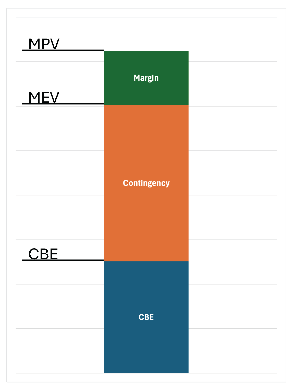
Figure 5.
Analyzed missions: (a) Sprite V1 and V2 [50], (b) PCBSat [51], (c) SpaceChip [52], (d) LuxAtto [53].
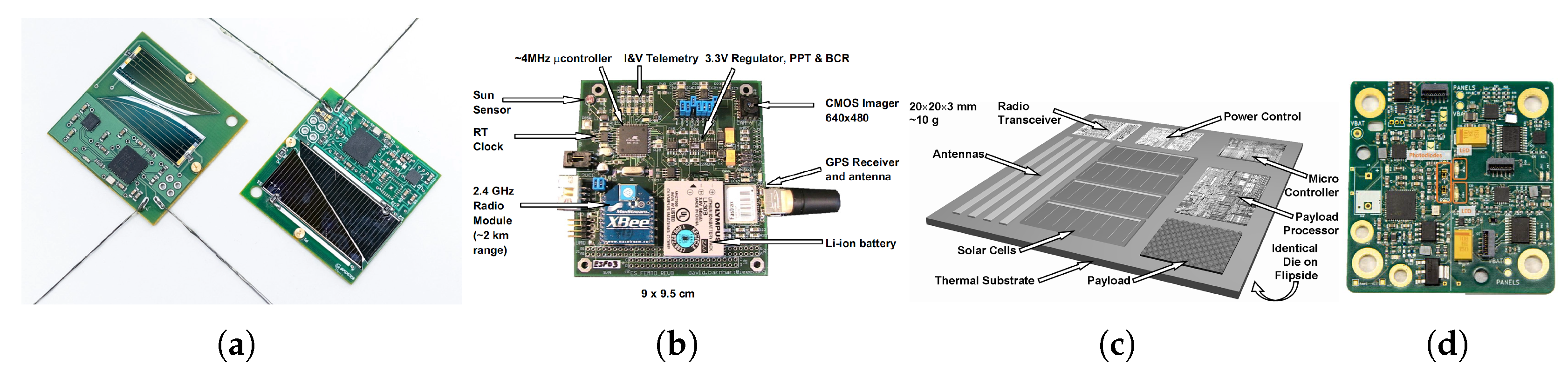
Figure 7.
Solar panel sizing and operational power envelopes for PlanarSat architectures. (a) Cumulative power sizing from CBE to MEV to MPV . (b–d) Operational envelopes for separated, mixed, and half-mixed designs sized to MEV; (e–g) same designs sized to MPV. The maximum incidence angle for full operation is indicated in each case.
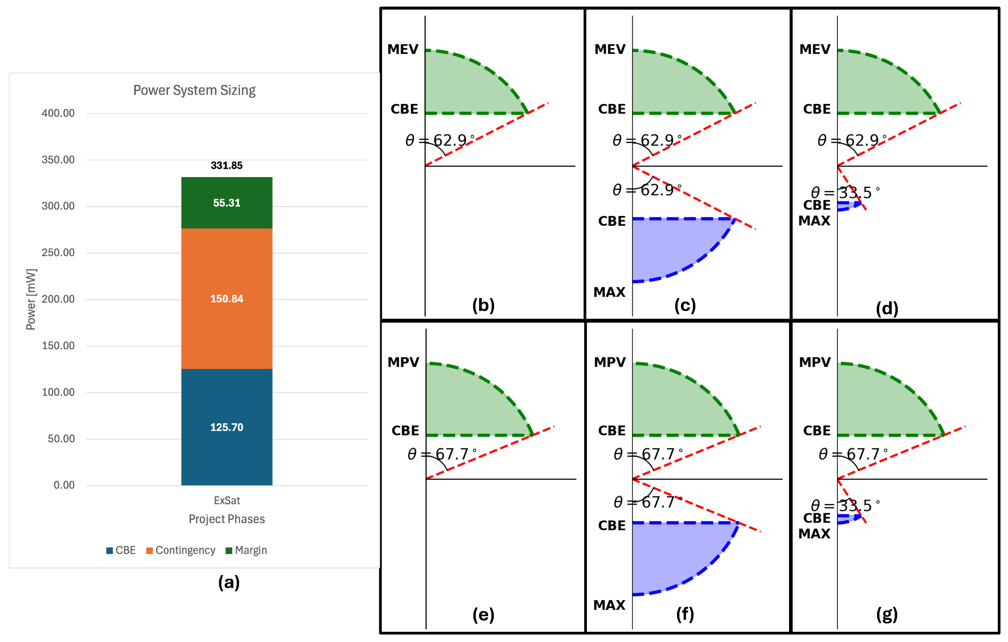
Table 6.
Extended recommended power contingencies based on AIAA minimum standard reserves [30]. Original anchors are retained; italicized entries are extrapolated for the refined low-power bins. “Bid” = Proposal phase; CoDR = Concept Design Review; PDR = Preliminary Design Review; CDR = Critical Design Review; PRR/FRR = Production/Flight Readiness Review. Class definitions follow [9]. The full set of unrounded values appears in Table A1 (Appendix).
| Proposal Stage | Design Development Stage | |||||||||||||||||
| Bid | CoDR | PDR | CDR | PRR/FRR | ||||||||||||||
| Class | Class | Class | Class | Class | ||||||||||||||
|
Description/ Categories |
I | II | III | I | II | III | I | II | III | I | II | III | I-II-III | |||||
| 0-1.2W | 120 | 65 | 13 | 105 | 50 | 12 | 70 | 45 | 9 | 45 | 40 | 7 | 5 | |||||
| 1.2-5W | 115 | 60 | 13 | 100 | 45 | 12 | 65 | 40 | 9 | 40 | 35 | 7 | 5 | |||||
| 5-20W | 110 | 55 | 13 | 95 | 40 | 12 | 60 | 35 | 9 | 35 | 30 | 7 | 5 | |||||
| 20-50W | 105 | 50 | 13 | 90 | 35 | 12 | 55 | 30 | 9 | 30 | 25 | 7 | 5 | |||||
| 50-100W | 100 | 45 | 13 | 85 | 30 | 12 | 50 | 25 | 9 | 25 | 20 | 7 | 5 | |||||
| 100-500W | 90 | 40 | 13 | 75 | 25 | 12 | 45 | 20 | 9 | 20 | 15 | 7 | 5 | |||||
| 500-1500W | 80 | 35 | 13 | 65 | 22 | 12 | 40 | 15 | 9 | 15 | 10 | 7 | 5 | |||||
| 1500-5000W | 70 | 30 | 13 | 60 | 20 | 12 | 30 | 15 | 9 | 15 | 10 | 7 | 5 | |||||
| 5000W + | 40 | 25 | 13 | 35 | 20 | 11 | 20 | 15 | 9 | 10 | 7 | 7 | 5 | |||||
Table 9.
Solar cell characteristics and power sizing details for analyzed missions [51,52,53,56,59]. For Sprites, “Max Power Generation” refers to per-side normal-incidence values. PCBSat and SpaceChip also report values sized at 45° those appear in the “Solar Sized for Power” row.
| Specification / Satellite | Sprite V1 | Sprite V2 | PCBSat | SpaceChip | Lux-P | Lux-A&B |
|---|---|---|---|---|---|---|
| Power and Sizing | ||||||
| CBE [mW] | 126 | 114 | 746 | 1.14 | 462 | 70 |
| Total Solar Cell Area [cm2] | 4.55 | 2.6 | 56 | 2.28 | 7.36 | 3.68 |
| Max Power Generation [mW] | 123 | 68 | 1131 | 1.87 | 105.2 | 52.6 |
| Solar Sized for Power [mW] | N/A | N/A | 821 (@45o) | 1.34 (@45o) | N/A | N/A |
| Satellite Dimensions [cm×cm] | 3.5×3.5 | 3.5×3.5 | 9×9.5 | 2×2 | 5×2.5 | 2.5×2.5 |
| Solar Cell Characteristics | ||||||
| Cell Efficiency [%] | 27 | 28 | 15 | 1 | 25 | 25 |
| Power Density [mW/cm2] | 27 | 26.15 | 15.88 | N/A | 14.3 | 14.3 |
| Cell Technology | Triple-J GaAs | Triple-J GaAs | Silicon | N/A | Silicon | Silicon |
Disclaimer/Publisher’s Note: The statements, opinions and data contained in all publications are solely those of the individual author(s) and contributor(s) and not of MDPI and/or the editor(s). MDPI and/or the editor(s) disclaim responsibility for any injury to people or property resulting from any ideas, methods, instructions or products referred to in the content. |
© 2025 by the authors. Licensee MDPI, Basel, Switzerland. This article is an open access article distributed under the terms and conditions of the Creative Commons Attribution (CC BY) license (http://creativecommons.org/licenses/by/4.0/).
Copyright: This open access article is published under a Creative Commons CC BY 4.0 license, which permit the free download, distribution, and reuse, provided that the author and preprint are cited in any reuse.


