Submitted:
27 June 2025
Posted:
30 June 2025
Read the latest preprint version here
Abstract
This paper presents a systematic, power-driven systems engineering approach for PlanarSats and the broader class of atto-, and femto-satellites, which are fundamentally constrained by extreme miniaturization and limited surface area for power generation. We reviewed existing space agency standards (NASA, ESA, JAXA) and the AIAA framework, identifying key limitations of current margin and contingency practices for highly miniaturized satellites. Based on these insights, we introduce an extended, log-linear methodology for determining phase- and class-appropriate power contingencies. The study defines power subcategories relevant to highly miniaturized platforms and demonstrates, through both historical and conceptual mission analyses, how application of these contingency values enables robust, reliable sizing of power systems. Detailed case studies show the direct relationship between power requirements, available surface area, and operational envelope, and provide practical methods for balancing requirement-driven and constraint-driven design. The results highlight that allocating surface area between solar arrays and electronics requires careful trade-offs. Additionally, the analysis demonstrates that using phase-aware margin management is essential for reducing risk and avoiding under-designed systems. This approach is intended to help designers optimize PlanarSat missions for reliability and efficiency under severe physical constraints. It also aims to provide a foundation for future advancements in highly miniaturized satellite architectures.
Keywords:
planarSat
; attosat
; femtosat
; small satellite
; chipSat
; systems engineering
1. Introduction
Satellite design is fundamentally governed by four constraints: mass, volume, power, and data. Mass is dictated by launch cost, volume by available fairing size, power by the satellite’s ability to generate and store energy, and data by mission objectives. Standardized form factors such as CubeSats and PocketQubes have enabled cost-effective access to space by imposing mass and volume limits; for example, per CubeSat and per PocketQube [1,2].
As the miniaturization of satellites continues, new architectures such as PlanarSats have emerged. PlanarSats are flat satellites with a surface area far larger than their thickness, where the challenge of generating sufficient power on a limited surface becomes dominant. Despite their unique geometry, PlanarSats must provide all core satellite functionalities, though subsystem scaling and layout differ from conventional satellites to fit the planar form factor [3].
A clear, structured approach for PlanarSat system development and design methodology is not yet available in the literature [3]. As reviewed in [3], the PlanarSat concept is introduced, with a survey of atto- and femto-satellites, including their dimensions, missions, power, and mass. Kanavouras et al. propose an agile systems engineering methodology for sub-CubeSat spacecraft such as femto- and atto-satellites, enabling rapid development cycles with reduced cost and increased flexibility compared to traditional approaches [4,5]. Ekpo and George introduce a deterministic, multifunctional architecture for highly adaptive small satellites, facilitating reconfigurable designs that yield significant mass and power savings [6,7]. Although these works are not focused specifically on PlanarSats, they provide a general, parametric approach to small satellite design, incorporating “mass” as a key variable based on textbook references [8,9].
The critical challenge for PlanarSats, as for other highly miniaturized platforms, is that as satellites shrink, the available surface area for solar cells decreases rapidly, yet all essential functionalities (processing power, data storage, communication, power systems, payload) must still be included. Literature consistently shows that power budgeting errors are a leading cause of mission failures in small satellites [10,11,12], underscoring the need for a design methodology that prioritizes power from the outset [13,14].
One key advantage of PlanarSats is their simple, two-dimensional geometry, which allows direct, empirical analysis of power generation and consumption. Leveraging established guidelines from organizations such as AIAA, NASA, and ESA, it is possible to build a more systematic and robust design process, including the integration of recommended contingencies and margins at every stage of design to ensure mission success.
Extreme miniaturization requires consolidating all essential subsystems; including power, communication, data handling, attitude control, and payload; are consolidated onto a single substrate (typically a single PCB),along with the remaining electronic components, with careful allocation of both surface area and power. Figure 1 illustrates how, as satellites shrink, required functionalities remain but the available power generation area diminishes, forcing trade-offs between satellite size, capability, and operational robustness.
This study addresses the lack of a tailored PlanarSat design methodology by developing a structured, power-driven approach for atto- and femto-satellites. Through systematic review and extension of contingency and margin standards, we introduce refined power categories and contingency scaling, and demonstrate their application on both real and conceptual missions. The result is a tailored, practical, quantitative method for sizing and optimizing PlanarSat architectures for robust operation.
2. Power-Based Satellite Design
A straightforward consequence of the PlanarSat form factor is that the available surface area is limited for both power generation and electronics. As a result, a design approach that centers on power generation and consumption enables a direct, iterative process for developing the satellite.
In this work, the sizing methodology is inherently bottom-up: starting from the power requirements and constraints imposed by the available surface area and known subsystem needs, and building up the overall design accordingly. This approach is motivated by the fact that, for PlanarSats and other ultra–small satellites, there is little historical or statistical data to support traditional top-down methods; such as those used for larger spacecraft, where mission–level payload requirements drive the design. Instead, this study generates new power categories and contingency guidance tailored specifically for these emerging satellite classes.
Contingency factors are considered at each design phase, and the satellite design is iteratively updated as the design matures. To provide a foundation for the methodology, the project phases and power margin recommendations from ESA, NASA, and JAXA are reviewed and summarized in Table 3 ((see also Table 1 and Table 2 for definitions and calculation steps). These margins are defined independently of satellite size, but vary according to design maturity, product evolution, and system risk, with changes tracked at key project milestones such as PDR, CDR, and PSR. In addition, AIAA provides recommended power contingencies based on both project phase and satellite power category, as shown in Table 4.
To interpret Table 3 and the methodology developed in this work, it is necessary to clarify how ’margin’ and ’contingency’ are defined and used in key agency standards and leading textbooks. The following subsection summarizes these definitions.
2.1. Margin and Contingency: Agency and Textbook Definitions
The use of margin and contingency is fundamental to spacecraft design, especially for power budgets in small satellites. However, the meaning, calculation, and application of these terms vary across major space agencies and standard references, which can lead to confusion in comparing methodologies or interpreting published values. This subsection summarizes the approaches of NASA, ESA, SMAD, and ESD, emphasizing their application to power budgeting and the rationale for the approach adopted in this study.
NASA: NASA distinguishes clearly between contingency (sometimes called growth allowance) and margin. Contingency is a percentage added to the CBE to account for uncertainty, especially in early design phases or for less mature technologies. The sum (CBE + contingency) is called the maximum expected value (MEV). Contingency percentages decrease as the design matures and uncertainty is reduced (e.g., 30–40% in early phases, 10–20% at PDR, 5–10% at CDR), Table 3. Margin refers to any additional buffer above MEV, sometimes defined for worst-case or “never exceed” scenarios (MPV). However, for power systems, NASA guidelines recommend sizing only to the MEV and not applying a further margin, to avoid “contingency pile-up”, Figure 2 [24,25]
ESA: ESA uses the term margin more broadly, sometimes encompassing both uncertainty allowances (contingency) and reserves. ESA typically applies a margin (e.g., 20% at the system level in early design phases) to the CBE, with margins decreasing as the design matures (e.g., 5–10% at CDR), as shown in Table 3. ESA engineering standards warn against double-counting: margins should not be added at both subsystem and system levels unless explicitly tracked and justified [26].
AIAA: The AIAA provides clear guidance on both contingency and margin. In the context of spacecraft power systems, S-122-2007 [27] and G-020-1992 guide [28] recommend applying contingency factors (multiplicative uplifts, typically 1.1–1.3 for initial estimates) to the current best estimate (CBE) of each subsystem’s demand to account for uncertainty, immaturity, and expected requirement growth [27]. These factors decrease as the design matures (e.g., 1.05 for qualification, 1.02 for measured/flight units), and should be "burned down" as more is known.
AIAA also defines a separate system margin [27], typically 5–20%, which is only applied after all contingencies are accounted for, and is reserved for worst-case or stress-test scenarios, not for routine sizing. The guide emphasizes that margin should not be added on top of contingency except for special cases, to avoid double counting or "margin pile-up." For most design and flight purposes, the Maximum Expected Value (MEV)—CBE plus contingency—is the appropriate target for sizing, while the Maximum Possible Value (MPV)—which includes an additional system margin—may be used for bounding or stress testing. These conventions are reflected in Table 4 and Table 1 of this paper.
SMAD: SMAD defines margin as “the amount by which the capability of a system exceeds the requirement,” and contingency as a percentage added to early estimates to address unknowns. Both are recommended in early design but are reduced as the project matures and uncertainties decrease [29].
ESD: ESD (based on AIAA guidelines, Table 4) also recommend adding a percentage margin (contingency) to CBE for sizing, but reporting conventions sometimes differ. ESD examples often report the final “margin” as a fraction of the built capability, i.e., (capability − CBE)/capability. This reporting style can make margins appear smaller and may confuse readers if not clearly explained. For sizing, ESD’s underlying process is the same as NASA/ESA: apply margin/contingency to CBE for each subsystem, sum, and size the system accordingly [9].

Table 1.
Summary of Contingency and Margin Features in System Analysis.
| Feature | Contingency | Margin |
|---|---|---|
| Applied to | CBE (estimated demand/cost) | Difference between supply/capability and MEV (demand + contingency) |
| Covers | Known unknowns, estimating errors, expected growth | Unknown unknowns, unforeseen events, design robustness |
| Management | Subsystem/team level | Project/program level |
| Trend | Decreases as uncertainties are resolved ("burns down") | Should remain positive, indicating design safety |
In this work, all contingency percentages are applied to the CBE for each subsystem, following NASA, ESA, and SMAD conventions. The resulting MEV is used to size the PlanarSat’s power system, avoiding further system-level margins to prevent excessive overdesign. This approach ensures clarity, robustness, and direct compatibility with agency review processes. Alternative reporting conventions (e.g., ESD’s fraction-of-capability margin) are noted for completeness but not used for sizing.
Key Definitions and Differences, as detailed in Table 1
- Contingency: An allowance (usually a percentage) added to the CBE of a project’s needs to cover known unknowns, expected but undefined growth, or estimating uncertainty. Managed at subsystem or team level and intended to "burn down" as the project matures and confidence grows.
- Margin: The difference between designed capability (supply) and the contingency-inclusive demand MEV. Provides a strategic buffer for unknown unknowns and design robustness; managed at the system or program level.
Relationship to Power Budgeting, as detailed in Table 2
- For power system sizing, best practice is to apply contingency to each subsystem’s CBE, sum the resulting MEVs, and size the system accordingly.
- Margin (in excess of MEV) is typically only added for bounding analyses or special requirements—not for routine sizing, to avoid “contingency pile-up.”
Note: If required by mission specification or for special stress tests, an additional system-level margin can be added to the MEV to define the MPV. This approach is reserved for worst-case or “never-exceed” scenarios; for standard satellite sizing, MEV remains the primary design target.
The design categories outlined in Table 4 [30] include: class I, which refers to a completely new spacecraft (unique and first-generation); class II, representing the next generation of spacecraft that builds upon a previously established design, offering increased complexity or capability within the same framework; and class III, which is a production-level model derived from an existing design, intended for multiple units with a significant degree of standardization [9]. These values are derived from a review conducted by AIAA, which examined historical data from previous NASA and DOD programs to develop industrial guidelines for the power margin presented in Table 4 [30]. Design maturity is defined based on the major reviews conducted during the design process, including the bid, CoDR, PDR, CDR, PRR, and FRR, as outlined in the same table.
Table 2.
Summary of CBE, MEV, and MPV for Power System Analysis.
| Term | What it Means | How to Calculate | Typical Use |
|---|---|---|---|
| CBE | Best estimate (today’s design) | Engineer’s calculated value | Baseline, preliminary analysis |
| MEV | Maximum expected value (with contingency) | CBE × (1 + contingency %) | Power system sizing |
| MPV | Maximum possible value (with margin) | MEV × (1 + margin %) | Stress/bounding, risk assessment |
Table 3.
Power Margins by Agency and Project Phase.
| Agency | Project Phase | Power Margin | Report Timing | Reference(s) |
|---|---|---|---|---|
| ESA | Equipment Level (Off-The-Shelf A/B) | ≥5% | During design and development | [31,32,33] |
| ESA | Equipment Level (Off-The-Shelf C) | ≥10% | During design and development | [31,32,33] |
| ESA | Equipment Level (New Design/Major Modification D) | ≥20% | During design and development | [31,32,33] |
| ESA | System Level (General) | ≥20% of nominal power | Throughout project lifecycle | [31,33] |
| ESA | System Level (IOD CubeSat at PDR) | 20% | At Preliminary Design Review (PDR) | [31,33] |
| ESA | Pre-PDR | 20% | Before Preliminary Design Review (PDR) | [31,33] |
| ESA | Pre-CDR | 10% | Before Critical Design Review (CDR) | [31,33] |
| ESA | At PDR | 5-15% | Preliminary Design Review (PDR) | [31,33,34] |
| ESA | At CDR | 5-15% | Critical Design Review (CDR) | [31,33,34] |
| NASA | Phase B (Formulation) | 30% | During Preliminary Design Phase | [35,36] |
| NASA | Initial Design (SMAD Recommendation) | 25% | Initial design phase | [35,36] |
| NASA | Historical Average (Aerospace Corporation Study) | 40% | Throughout design phases | [35,36,37] |
| NASA | At PDR | 20% | Preliminary Design Review (PDR) | [35,36] |
| NASA | At CDR | 10% | Critical Design Review (CDR) | [35,36] |
| JAXA | PDR (New bus & payload) | 15% | At Preliminary Design Review (PDR) | [36,38,39] |
| JAXA | CDR (New bus & payload) | 10% | At Critical Design Review (CDR) | [36,38,39] |
| JAXA | PSR (New bus & payload) | 6% | At Post-Shipment Review (PSR) | [36,38,39] |
| JAXA | PDR (Large changes to existing bus/payload) | 10% | At Preliminary Design Review (PDR) | [36,38,39] |
| JAXA | CDR (Large changes to existing bus/payload) | 8% | At Critical Design Review (CDR) | [36,38,39] |
| JAXA | PSR (Large changes to existing bus/payload) | 6% | At Post-Shipment Review (PSR) | [36,38,39] |
| JAXA | PDR (Minor changes to existing bus/payload) | 5% | At Preliminary Design Review (PDR) | [36,38,39] |
| JAXA | CDR (Minor changes to existing bus/payload) | 8% | At Critical Design Review (CDR) | [36,38,39] |
| JAXA | PSR (Minor changes to existing bus/payload) | 4% | At Post-Shipment Review (PSR) | [36,38,39] |
| JAXA | PDR (Existing bus & payload) | 5% | At Preliminary Design Review (PDR) | [36,38,39] |
| JAXA | CDR (Existing bus & payload) | 5% | At Critical Design Review (CDR) | [36,38,39] |
| JAXA | PSR (Existing bus & payload) | 3% | At Post-Shipment Review (PSR) | [36,38,39] |
The AIAA power categories offer a well-structured framework for scaling power contingencies based on satellite size and power capacity. This approach is particularly beneficial for smaller satellites, where power resources are more constrained. Smaller satellites are more likely to encounter challenges such as power degradation, inefficiencies in power generation, and limitations in redundancy, which makes them vulnerable to failure if not properly designed. The AIAA framework scales contingencies to ensure that smaller satellites receive higher margins as their available power decreases, compensating for these specific risks. This scaling of contingencies directly addresses the unique challenges posed by smaller satellites, providing them with a buffer against power-related uncertainties that could jeopardize mission success. By relying on historical mission data and empirical evidence from NASA and DOD programs, the AIAA system offers a more specific method for determining appropriate power contingencies than many other space agencies, which use broader, less specific contingency guidelines.
Table 4.
AIAA recommended minimum standard power contingencies in %. Category descriptions are taken directly from the reference [9,28,30].
| Proposal Stage | Design Development Stage | ||||||||||||||
|---|---|---|---|---|---|---|---|---|---|---|---|---|---|---|---|
|
Bid Class |
CoDR Class |
PDR Class |
CDR Class |
PRR Class |
|||||||||||
| Description/ Categories |
1 | 2 | 3 | 1 | 2 | 3 | 1 | 2 | 3 | 1 | 2 | 3 | 1 | 2 | 3 |
| Category AP 0-500 W |
90 | 40 | 13 | 75 | 25 | 12 | 45 | 20 | 9 | 20 | 15 | 7 | 5 | 5 | 5 |
| Category BP 500-1500 W |
80 | 35 | 13 | 65 | 22 | 12 | 40 | 15 | 9 | 15 | 10 | 7 | 5 | 5 | 5 |
| Category CP 1500-5000 W |
70 | 30 | 13 | 60 | 20 | 12 | 30 | 15 | 9 | 15 | 10 | 7 | 5 | 5 | 5 |
| Category DP 5000 W and up |
40 | 25 | 13 | 35 | 20 | 11 | 20 | 15 | 9 | 10 | 7 | 7 | 5 | 5 | 5 |
In comparison, other values shown in Table 3 often apply broader margin values across different mission types. For instance, ESA’s typical 20% power margin for all system levels does not adjust for the specific risks associated with smaller satellites, which require more tailored contingencies/margins to address the higher likelihood of power-related issues in lower-power systems. The AIAA model, on the other hand, adjusts power margins based on satellite power levels, ensuring a more flexible and scalable framework for relatively smaller satellite mission planning. This adaptability makes the AIAA model particularly suitable for the evolving field of small satellites, especially with the growing number of smaller and more power-constrained systems.
However, the current categories, especially the 0-500 W range, do not fully address the needs of nano, pico, femto, and atto satellites, which face unique challenges and power constraints. One of the goals of this research is to propose a refined methodology for these lower-power categories and develop more detailed power margin values tailored to these highly miniaturized satellites. Given the lack of accumulated data for these smaller categories, this approach will first establish a methodology for determining power contingencies and then demonstrate how contingency values will be generated to support the newly proposed categories. As technology advances and these smaller satellite classes continue to evolve, the proposed framework will ensure that they are accounted for with accurate power contingency/margin estimates, keeping the system adaptable and relevant for future missions across diverse satellite classes.
2.2. Definition of Power Subcategories
The lowest power category in established frameworks such as AIAA is 0–500 W, Table 4 [9,28]. However, PlanarSats and other highly miniaturized satellites operate at far lower power levels, requiring a more granular set of categories. To establish physically meaningful bins in this range, we begin by analyzing standardized satellite classes, CubeSats and PocketQubes, using a representative commercial solar cell (4×8 cm, ∼30% efficiency, 1.2 W maximum output at normal incidence) [40]. By mounting these cells on each satellite face and assuming simultaneous solar illumination at 45° incidence on three surfaces, the maximum achievable power for each class is estimated, as summarized in Table 5.
Analysis of the resulting power levels indicated that the conventional AIAA bins (e.g., 0–500 W) are too coarse for the highly miniaturized satellite regime. However, a four-level breakdown (50–20 W, 20–5 W, 5–1.2 W, 1.2–0 W) is found to align well with both the curve, shown in Figure 3, of achievable power and the geometric progression observed in the AIAA table’s middle values. The lowest boundary was also adjusted from 500–100 W to 500–0 W to ensure full granularity for the smallest systems.
Combining the original and extended bins yields a refined set of categories: 5000+ W, 5000–1500 W, 1500–500 W, 500–100 W, 100–50 W, 50–20 W, 20–5 W, 5–1.2 W, and 1.2–0 W. The 100–50 W category bridges the gap between the existing AIAA categories and the newly defined bins. Figure 3 visualizes this updated categorization, using geometric means for bin centroids to facilitate log-linear extrapolation in subsequent contingency estimation.
The upper limit for the power range (5000+ W, set at 50 kW for plotting) is shown for completeness and context, referencing large systems such as the ISS (up to 248 kW at BoL) and Tiangong Space Station (max 55 kW) [41,42]. However, the focus of this study remains on the lower end, where PlanarSats and other highly miniaturized classes dominate, and where the proposed fine-grained bins support more tailored/specific contingency estimation. The chosen subcategories thus offer a practical starting point for extrapolation and margin methodology in the absence of comprehensive historical data, and are intended as engineering guidelines for future work on highly miniaturized satellites.
2.3. Investigation of Contingencies for Lower Power Categories
Due to the lack of historical data for highly miniaturized satellites, contingency values for the lower power ranges must be extrapolated beyond the established AIAA table. Instead of adopting generic margin values from ESA, JAXA, or NASA; which do not account for the unique risks and trends of highly miniaturized satellite missions, we extend the AIAA methodology to define more granular power categories. This provides a consistent, power-centric framework specifically designed for the new generation of highly miniaturized spacecraft.
To estimate contingency values for each new power category, several interpolation schemes were evaluated. Linear-linear interpolation (contingency as a linear function of power), log-log interpolation (both axes in log scale), and higher-order methods such as splines or piecewise binning were considered but ultimately rejected. These approaches either poorly reflect the trend across orders of magnitude or introduce nonphysical artifacts and discontinuities.
Instead, a log-linear approach where contingency varies linearly with the logarithm of power, was selected. This method best represents the exponential decay in uncertainty as satellite power increases, is robust for data spanning multiple decades, and matches established practices in aerospace engineering for handling skewed datasets. Empirical inspection of anchor points and validation against known contingencies confirmed that log-linear interpolation yields plausible intermediate values consistent with engineering experience.
Instead, we selected a log-linear approach, where the contingency varies linearly with the logarithm of power. The anchor points for this extrapolation are based on published AIAA contingency recommendations for small satellites, as shown in Table 4. Although these anchor points are limited, especially for the lowest power categories, extrapolating from them provides intermediate values that follow a consistent trend with the available data. Due to the lack of direct historical data for femto- and atto-satellite classes, these results should be considered as practical engineering estimates. They serve as initial guidelines and should be refined as additional mission data becomes available.
For the lowest bin (0–1.2 W), a lower bound of 0.1 W is set to avoid . The geometric mean of each bin’s endpoints,
is used as the representative power for extrapolation. Here, and represent the lower and upper bounds of the power bin, respectively. The extrapolated contingency at is then calculated as:
where and are adjacent known data points.
By applying this approach to the previously available AIAA contingencies, shown in Table 4 [28], we are able to generate the new extended contingencies shown in Table 6. All contingency values in Table 6 were calculated and extrapolated in logarithmic space to ensure consistency across orders of magnitude. For clarity and practicality in engineering application, the final recommended values were rounded to the nearest integer. The values in parentheses show the unrounded results. This methodology enables the systematic and transparent extension of contingency recommendations into power ranges where historical data is limited or absent, supporting robust and realistic PlanarSat design.
One notable outcome of our extended contingency table is the appearance of contingency values exceeding 100% for low-power, Class I designs; especially in the earliest design phases (Bid, CoDR). For example, a 140% contingency is assigned for Class I (see Table 4 for full class definitions) Bid at 0–1.2 W, with similarly high values in neighboring bins. While these levels may appear excessive, they are well supported by both agency guidance and observed mission histories for novel or highly constrained systems. In such cases, a contingency above 100% simply means the system should plan for more than double the nominal power estimate; a reasonable step when initial requirements, new technologies, or severe size constraints drive high uncertainty.
Major space agencies all recognize circumstances where such high contingency is justified. NASA standards, for example, explicitly allow up to 100% contingency for early-phase or first-of-kind subsystem designs, and “2×” (100%) rules are often cited for unknown or unproven technologies [43,44]. Studies by Aerospace Corp. and recent NASA probe missions have documented average power growth of 40–75% across design phases—sometimes higher for innovative payloads [45,46]. ESA, though typically capping system-level margins at 20% in mature phases, allows much more in Phase 0/A when requirements are uncertain, with case-by-case contingency allocations that may exceed 100% for new payloads [26]. JAXA also advocates the accumulation of large margins (up to 150–200%) for early, small, or experimental missions, reflecting the compounded uncertainty in each subsystem [47]. Similar findings appear in smallsat literature, where mission failures are often traced to underestimation of power needs or unexpected system growth [48,49].
Importantly, these extreme contingencies are limited to early-phase, high-uncertainty cases—by the time a mission reaches PDR or CDR, design maturity and confidence bring contingencies below 100%, as shown in Table 6 and consistent with industry practice [43,50]. The methodology of log-linear extrapolation and geometric mean binning captures both the initial risk and its progressive reduction as designs evolve.
In summary, contingency values above 100% are a rational response to the high risk inherent in early, low-power, or novel designs. They serve as a practical warning and a robust buffer, ensuring adequate power system sizing in the face of profound uncertainty.
To demonstrate the practical application of this framework, the next section presents case studies using published power data from a range of state-of-the-art femto–and atto–satellites.
3. Case Study: Application to Real/Conceptual Satellites
To illustrate the application and value of the proposed methodology, this section analyzes several representative PlanarSats, in the femto- and atto-satellite category. For each case, power requirements and generation methods are summarized, appropriate margin categories and design phases are identified, and the methodology is used to derive recommended design values. The performance of each mission is then briefly assessed in the context of the new framework.
Figure 4.
Analyzed Satellite Missions: (a) Sprite V1 and V2 [51] (b) PCBSat [52]. (c) SpaceChip [53] (d) Univeristy of Luxombrough, SpaceChip V1[54], to prevent confusion it will be referred as LuxAtto in this paper.
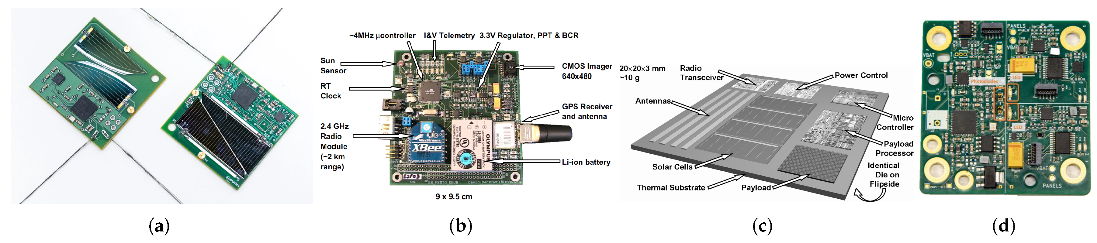
Five missions have been selected for the case study:
- Sprite V1 and V2,Figure 4(a): Version numbers are given in this paper to distinguish the satellites, which were onboard on Kicksat-1 and 2 missions, respectively. Maximum power consumption is calculated from respective BOM and datasheets, approximately and . Although both satellites were launched/deployed, Sprite V1 is classified as a Class 1 mission (first-of-kind, no prior heritage) and Sprite V2, benefiting from V1’s flight experience, is assigned to Class 2, according to Table 6. Both satellites are analyzed at CDR, typically the final opportunity to adjust power system sizing before hardware is frozen [21,55,56,57].
- PCBSat and SpaceChip,Figure 4(b) and (c): Designed by Barnhart et al., these are conceptual studies; only PCBSat was partially realized as an early concept. Power requirements are (PCBSat) and (SpaceChip). Both are Class I, with PCBSat analyzed at CoDR phase (physical prototype manufactured) and SpaceChip at Bid phase (feasibility study) [52,53].
- University of Luxembourg’s Chipsat V1 (LuxAtto),Figure 4(d): An early concept of University of Luxembourg’s Chipsat V2, which was launched in January 2025. Power consumption is (LuxAtto P, primary) and (LuxAtto A&B, secondary). The LuxAtto satellites are analyzed separately: the primary as Class II (heritage from Sprite V1) at PDR, and A&B as Class I at PDR (new, smaller form factor), with an iteration launched on POQUITO in January 2025 [54,58,59].
Using the contingency values in Table 6, MEV for each satellite is calculated. To prevent cascading of margins and contingencies as discussed in [24], additional margins were not added. The sizing of the satellites, particularly the solar cells/arrays, should be done according to MEV values. Table 7 summarizes the classification (by mission class and design phase), CBE, contingency applied, and resulting MEV for each satellite analyzed.
Contingency is applied to the CBE of power demand before solar array sizing. The resulting MEV defines the required power generation capacity. The solar array is then sized directly to meet or exceed this value, ensuring adequate margin for design uncertainties and early-phase estimation errors. The MEV values in Table 7 serve as the solar array sizing recommendation. Sizing below this threshold does not necessarily prevent satellite operation but will limit performance, such as data generation and transmission capability. Undersizing, however, is a frequent cause of smallsat mission underperformance or failure, as found in multiple survey studies [10,11,12].
According to the calculated MEV in Table 7, the recommended solar array sizing for PCBSat is . This is more than twice the nominal value of reported for the actual satellite [52]. The satellite’s CBE was , with additional factors such as power conversion efficiency and a solar incidence angle included in the analysis [52]. Given PCBSat’s maximum power generation capability of , the design as flown effectively included a margin over the CBE. However, had the system been sized for the MEV (), operational time would have likely improved. This improvement is due to the ability to generate additional power, especially considering that the initial design assumed a solar incidence angle. In practice, this angle could increase up to , which would enhance power generation and, consequently, extend the satellite’s operational time. As the satellite did not include an ADCS and was expected to tumble freely, any additional power generation directly enhances the satellite’s operational duty cycle. This example demonstrates the use of the margin methodology for future design applications.
The sizing of the SpaceChip power system was performed similarly [52,53]. The solar cell referenced in Table 8 assumes an efficiency of . The calculated MEV is , which is higher than the initial sizing value of (originally sized for at ). Considering this sun angle and system power conversion efficiency [52], the satellite would have a maximum possible power generation with a margin under ideal conditions, based on the initial CBE of . If the satellite were designed for the calculated MEV, as in PCBSat, it would allow for of sunlight incidence. Since this satellite has no ADCS and is free-tumbling, its operational average output per orbit would increase, allowing for more data to be collected and transmitted. A downside of MEV sizing is that it would increase the satellite size from to , representing a increase, assuming the same solar cell technology as reported by Barnhart [52].
The CBE for Sprite V1 and V2 were calculated based on the IC on the satellites [55,60]. Although their sizes and CBE values are similar, at and respectively, different solar cells were used on each satellite (see Table 8). The values provided are for a single surface only. Both satellites had solar cells on either side, allowing them to generate more average orbit power, even while tumbling. For Sprite V1, with a maximum solar power generation of on either side under direct sunlight, the satellite would face challenges, as its CBE of exceeds its maximum capability. Any deviation in the sun angle would cause a drop in power generation, directly affecting satellite operations; especially with the radio, which uses during transmission [55].
If the system were focused solely on transmission, it could handle a sun angle of incidence up to . With an MEV of , the satellite would be fully operational even with the initial CBE, and it could handle an angle of incidence of . When focused solely on transmission, this could increase to . Given that the satellite has solar cells on both sides, this would improve its operational envelope by about . However, the MEV would increase the satellite’s required area by , from to .
The effect is more drastic on Sprite V2, primarily due to the different solar cells used, as shown in Table 8 [60]. The calculated MEV for Sprite V2 is , which is lower than Sprite V1 due to the reduced contingency value based on the class under which Sprite V2 was considered. Despite this, there would still be an operational improvement, allowing for more average operational time at a CBE of , enabled by an increased incident angle of . When compared with the solar cells already included in the design, which generate on a single surface at a angle of incidence, the system could handle a transmission-focused scenario with an increased incident angle of , up from .
It should be noted that since the Sprite satellites have solar cells on both sides, the impact of the difference in solar array sizing will be more significant than the basic initial calculations suggest. This allows for a larger operational envelope in which the satellite can generate more power. However, to generate enough power for the MEV of , the satellite would need an additional of surface area, resulting in a increase from the initial surface area of .
Hypothetically, consider a satellite program called “Sprite Project,” comprising two missions, Sprite V1 and Sprite V2, as a continuous development effort. If Sprite V1 were evaluated at the PDR phase, with a CBE of , the recommended maximum expected value (MEV) would be , based on a contingency from Table 6. As the project evolves and enters the Critical Design Review (CDR) phase with Sprite V2, a lower contingency of is justified, yielding an MEV of for a refined CBE of . While the change in MEV between phases is not strictly a margin in the traditional sense, maintaining the original sizing would effectively provide a margin at CDR, as illustrated in Figure 5. This progression demonstrates how both design maturity and accumulated heritage enable a systematic reduction in contingency, resulting in a right-sized power subsystem for later missions. By applying this methodology, the Sprite Project can efficiently reduce overdesign and improve mass and cost efficiency while maintaining robust risk mitigation.
Similarly, for the LuxAtto satellites, the power that can be generated with their solar cells is less than their CBE, as shown in Table 8. This means the satellites rely on charging their batteries via solar power, later using battery energy for operations [54]. A design according to MEV (see Table 7) would allow the primary, referred to as Lux-P in this paper, to operate even during a solar angle of incidence of and enable faster battery charging, thus increasing operational time. A design based on MEV would increase the required surface area for Lux-P from to and for Lux-A&B from to at least.
It should be emphasized that these calculations are performed on already-built (i.e., "finished") satellite missions. Satellite engineering is fundamentally a series of trade-offs; improvements in one aspect may come at the cost of another. However, a structured approach to power budgeting, as demonstrated here, enables better-informed design decisions, improved estimation of mission outputs (such as data return), and more predictable planning of development cost and schedule.
While this study primarily considers surface area for power generation, it is important to note that increases in satellite volume can also affect design constraints. Greater volume may allow for additional subsystem integration, thermal management options, or battery inclusion, but may also increase mass and launch costs, and potentially complicate thermal or structural design. Therefore, volume expansion introduces its own trade-offs that must be balanced alongside power and surface area considerations.
For PlanarSats, power generation relies almost exclusively on solar panels mounted on the limited available surface. Thus, the derived MEV values directly determine the minimum required solar cell area, establishing a close relationship between power budget and physical geometry. Undersizing of power systems remains a primary risk for small satellites, but the use of a contingency-based, power-centric methodology can significantly reduce this risk and improve overall mission success.
These results demonstrate that applying phase- and class-appropriate contingency factors yields robust power system sizing, and that design maturity and mission heritage systematically reduce required contingencies. This structured approach directly supports improved mission reliability and efficiency for future PlanarSat and small satellite missions, as evidenced by historical failure analyses, agency recommendations, and the improved alignment of design capabilities with mission needs in the presented case studies [10,11,24,25,26].
In the following section, the direct relationship between power requirements and available surface area for solar cell placement is quantified, establishing the central trade-off in PlanarSat architecture.
4. PlanarSat System Development Approach
PlanarSats, by definition, are essentially two-dimensional satellites. Especially at the atto-, and femto-satellite levels, they tend to be a single substrate; most often a single PCB [3]. Power generation in such satellites depends on solar cells, which directly occupy some of the available surface. Depending on the chosen solar cell technology and efficiency, the required area will vary and can limit the surface available for other satellite functions. Conversely, to provide sufficient power, the satellite may need to be sized up to accommodate more solar cells, which in turn can increase the available area for other functionalities.
Notably, most PlanarSats, particularly in the atto- and femto- classes, do not include a battery, due to factors such as direct temperature exposure, additional cost (both financial and in protection circuit development time), and, most importantly, limited available volume. Given the single-plane structure and the possibility of using both surfaces, three initial satellite configurations are commonly considered. Depending on available resources and mission-criticality, designers may choose among these options.
These initial approaches are illustrated in Figure 6: (a) one side with solar cells only, the other with electronics only (“separated”), (b) one side with solar cells only, the other side with both solar cells and electronics (“half-mixed”), and (c) both sides with a combination of solar cells and electronics (“mixed”). These configurations each present distinct trade-offs. Sprite and ChipSat are mixed type; LuxAtto and PCBSAT are separated satellites. The basic PlanarSat architectures analyzed in this study are illustrated in Figure 6.
In the most basic scenario, assuming free-tumbling satellites, having solar cells on both sides increases the likelihood of generating power at any orientation. The main downside is cost, as space-qualified high-efficiency solar cells are expensive [3]. Performance can be further improved by incorporating an ADCS; for example, a two-axis magnetorquer, to sun-point and optimize power generation. However, this requires careful trade-off analysis, as the power consumed by the ADCS itself must be included in the system budget.
If such an attitude control system is implemented, each architecture responds differently:
- Separated: Highest risk; if the solar cell face is not sunward, there is no generation. Even partial sunlight may not be sufficient, and the convergence time of the ADCS will strongly affect performance. A backup battery or a fast-reacting control system may be necessary.
- Half-mixed: The smaller solar cell face can be used to keep the ADCS system powered, enabling controlled flipping so the larger cell face can point at the Sun, thus increasing power generation.
- Mixed: Offers the highest probability of sun-pointing from any orientation, providing more consistent power generation and enabling better mission planning. However, this approach increases the number of solar cells (and thus cost) and may require enlarging the satellite to compensate for increased power demand, which could affect launch opportunities or cost.
Each approach presents a unique balance between operational flexibility, system complexity, mass, and cost. The choice ultimately depends on mission priorities and constraints.
4.1. A PlanarSat Design: Operational Power Envelopes
The design of most current femto- and atto-class PlanarSats is based on practical experience and the available component set, as previously reviewed in [3]. Detailed design and system sizing is provided in studies [52,53] which are based on SMAD [29]. Unlike traditional satellites, these systems face a high degree of design uncertainty, with fewer established best practices due to limited mission heritage. This section demonstrates how the proposed contingency and margin methodology can directly inform PlanarSat sizing and operational analysis, using a realistic example.
Here, a top–down PlanarSat concept is developed to illustrate the process from CBE through MEV to MPV, as well as the inverse approach (sizing based on available resources). The selected components are: an MCU (STM32L496RGT3, , at ) [64], a transceiver (SX1278IMLTRT, , during transmit for RF output, during receive) [65], and a generic payload (, including peripherals). The satellite is assumed to operate in two primary modes: transmission (MCU + transmitter) and payload with receiver active; for this demonstration, receive is assumed always enabled except during transmission. The CBE for transmission is , placing it in the 0– category of Table 6. As a first-of-its-kind mission (Class I) and at the Bid phase, a contingency of is applied; to further illustrate the methodology, a margin is also included.
Table 9.
Representative component areas and references.
| Component | Area [cm2] | Reference |
|---|---|---|
| STM32L496RGT6 MCU | 1.96 | [64] |
| SX1278IMLTRT Transceiver | 0.49 | [65] |
| Example Payload | 2.00 |
The concept of an operational power envelope is proposed to capture how available incident solar power, satellite architecture, and sizing contingency/margin combine to determine the range of operational orientations for PlanarSats. Figure 7 illustrates how the maximum available power varies for each PlanarSat architecture as a function of the Sun’s incidence angle. The available solar power on a given surface can be approximated by
where is the maximum power at normal incidence and is the angle between the surface normal and the direction to the Sun. As shown in Figure 7, the maximum angle of incidence () at which the satellite remains fully operational is directly determined by the size of the solar array relative to the required power (MEV or MPV). For lower angles, power generation increases, offering surplus power for additional activities or increased system robustness.
Figure 7b–d present operational envelopes for the three baseline PlanarSat architectures (defined in Figure 6), using MEV as the sizing driver. In the separated case (b), a solar cell covers one side and all ICs are on the reverse; power can be generated only when the cell faces the Sun, limiting the operational envelope to within . In the mixed case (c), cells are placed on both sides along with electronics, providing operational capability in either orientation. The half-mixed design (d) allocates a full-sized cell to one side, and a smaller cell to the remaining area on the reverse; this results in a reduced operational angle on the small-cell side, corresponding to the CBE, and a maximum angle (MAX) determined by the area constraint.
Figure 7e–g repeat the analysis for systems sized to MPV, showing that larger margin allows for a greater operational angle; expanding the envelope and enabling more robust or flexible mission profiles, assuming a free-tumbling satellite with no ADCS. The 2D geometry assumption implies that rotation is dominated about the surface normal (Z-axis), with limited rotation in the X and Y axes due to atmospheric drag. Although designing the satellite with respect to the MPV seems beneficial from an operational point of view, it may lead to increased cost and size due to larger solar cells, and can introduce further challenges such as increased thermal and vibration sensitivity.
This design trade-off directly reflects the guidance from NASA’s concurrent engineering resource management philosophy, which cautions against overallocating margin “simply to reduce risk,” noting that excessive margins can drive unnecessary increases in system complexity, mass, and cost, with potential negative impacts elsewhere in the design [24]. Instead, margin and contingency should be “used judiciously and only when justified by real uncertainties,” with their values iteratively refined as the design matures [24].
This principle is not unique to NASA’s concurrent engineering philosophy; in fact, it is a central tenet of all power-focused satellite design. By explicitly balancing risk reduction with system complexity, mass, and cost, power-focused approaches inherently strive to use margin and contingency judiciously. The methodology presented here formalizes this balancing act for highly miniaturized systems, where the impacts of margin decisions are amplified due to tighter constraints.
In summary, the concept of the operational power envelope offers a tangible bridge between abstract power margin methodology and concrete hardware constraints in PlanarSat design. It enables rational decision–making about surface allocation and operational robustness, while highlighting the system–level consequences; both positive and negative, of design choices around contingency and margin. As the field moves toward ever-smaller satellites and more aggressive mission profiles, this structured approach will be crucial for balancing innovation, risk, and resource efficiency.
Sizing Example: Requirement-Driven vs. Constraint-Driven for Single-Sided PlanarSat
We now provide a worked example of the PlanarSat sizing process using typical component footprints and solar cell specifications. Here, we focus on the “one side cells, one side electronics” (separated) configuration (see Figure 7b,e), illustrating the effect of contingency (MEV) and margin (MPV).
(1) Requirement-Driven Sizing (Power First)
Suppose a PlanarSat design requires (MEV). Using the Azur Space 3G30A cell ( at AM0) [40], the minimum solar cell area needed is then:
Component footprints are assumed as follows: STM32L496RGT6 MCU () [64], SX1278IMLTRT Transceiver () [65], and payload with peripherals (). The total area required for electronics is
The total minimum side area is thus
The corresponding minimum side length for a square PlanarSat is . For worst-case or stress-test sizing (MPV), assuming a 20% additional system margin:
Minimum side length: .
(2) Constraint-Driven Sizing (Fixed Area First)
In the constraint-driven scenario, the satellite’s physical size may be set by a standard form factor (e.g., cm), providing ample power margin, or by the smallest manufacturable outline that just fits both the required electronics and solar cell area. For instance, a compact PlanarSat of cm provides of total surface area; sufficient for CBE–level operation, but with minimal excess for contingencies or non-idealities. This comparison highlights the direct trade-off between system compactness and operational robustness.
For a cm PlanarSat:
For a cm PlanarSat:
Table 10.
Summary of PlanarSat sizing for single-sided configuration (separated): requirement-driven and constraint-driven cases. Power generation values assume incidence angle.
Table 10.
Summary of PlanarSat sizing for single-sided configuration (separated): requirement-driven and constraint-driven cases. Power generation values assume incidence angle.
| Approach | Area (cm2) | Side Length (cm) | Max Solar Power (mW) |
|---|---|---|---|
| Constraint-driven (fixed cm) | 9.00 | 3.00 | 181 |
| Requirement-driven (MEV) | 11.99 | 3.46 | 300 |
| Requirement-driven (MPV) | 13.50 | 3.67 | 360 |
| Constraint-driven (fixed cm) | 25.00 | 5.00 | 817 |
This calculation demonstrates the direct, quantitative link between surface allocation, power margin methodology, and hardware feasibility in PlanarSat design. For both cases, actual operational power will be further reduced by incidence angle, temperature, and other losses; as such, the proposed approach offers a practical, engineering-relevant way to ensure system robustness at the femto/atto scale.
This quantitative approach provides a foundation for the next stage of PlanarSat design; allocating surface area among subsystems and optimizing power/data trade-offs under strict geometric constraints.
While this section demonstrates the core architectural trade-offs and their effects on power availability for PlanarSat-class systems, a full quantitative comparison between designs—including explicit surface allocation, phase-based contingency, and margin budgeting—is beyond the present scope. These detailed analyses will be addressed in future work, building on the foundation established here.
5. Conclusion and Future Work
This work introduced a structured, power-based systems engineering methodology for PlanarSats and the broader class of atto-, femto-, and pico-satellites. By systematically extending contingency and margin standards from NASA, ESA, JAXA, and AIAA, a refined, scalable framework was developed for a flexible and tailored power system sizing at the smallest scales.
Deatiled power subcategories and log-linear contingency extrapolation (Table 6) were established, enabling designers to select appropriate margins for novel, low-power missions. Application of this methodology to both historical and conceptual PlanarSat examples demonstrated how design maturity and mission heritage systematically reduce required contingencies and improve robustness (see Section 3, Table 7). The “operational power envelope” concept provided an explicit engineering link between margin philosophy, surface allocation, and mission feasibility at the femto- and atto-satellite scale (Figure 6 and Figure 7). The combined requirement-driven and constraint-driven sizing cases highlighted the direct, quantitative trade-offs that define PlanarSat surface utilization and mission capability.
Ultimately, the methodology proposed here offers a practical means to reduce the risk of under-designed power systems; a leading cause of failure in highly miniaturized satellites, while supporting scalable and robust mission planning as the field advances.
Future work will focus on expanding the empirical database for atto- and femto-satellites, refining margin recommendations as more missions are flown, and integrating additional system-level trade-offs—such as thermal, radiation, and structural constraints—into the power-surface design process. Further optimization of solar array, payload, and electronics co-placement, as well as demonstration on a complete PlanarSat design, will be pursued to provide a comprehensive and validated development approach for this emerging class of spacecraft.
Author Contributions
Conceptualization, M.S.U.; methodology, M.S.U.; software, M.S.U.; validation, M.S.U. and A.R.A.; formal analysis, M.S.U.; investigation, M.S.U.; resources, M.S.U.; data curation,M.S.U.; writing—original draft preparation, M.S.U.; writing—review and editing, M.S.U. and A.R.A.; visualization, M.S.U.; supervision, A.R.A.; project administration, M.S.U.; funding acquisition, M.S.U. and A.R.A. All authors have read and agreed to the published version of the manuscript.
Funding
This research received no external funding.
Institutional Review Board Statement
Not applicable.
Informed Consent Statement
Not applicable
Data Availability Statement
The original contributions presented in the study are included in the article, further inquiries can be directed to the corresponding author.
Acknowledgments
The authors thank Assistant Prof. Onur Çelik, Assistant Prof. Stefano Speretta and Dr. Erdem Turan for their feedback, comments and support.
Conflicts of Interest
The authors declare no conflicts of interest..
Abbreviations
The following abbreviations are used in this manuscript:
| ADCS | attitude determination and control system |
| AIAA | American Institute of Aeronautics and Astronautics |
| Bid | bidding |
| CBE | current best estimate |
| CDR | critical design review |
| CoDR | conceptual design review |
| DOD | Department of Defence |
| ESA | European Space Agency |
| ESD | Elements of Spacecraft Design |
| FRR | flight readiness review |
| IC | integrated circuit |
| JAXA | Japan Aerospace Exploration Agency |
| MCU | microcontroller |
| MDPI | Multidisciplinary Digital Publishing Institute |
| MEV | maximum expected value |
| MPV | maximum possible value |
| NASA | National Aeronautics and Space Administration |
| PCB | printed circuit board |
| PDR | preliminary design review |
| PRR | pre–ship readiness review |
| PSR | post–shipment review |
| SMAD | Space Mission Analysis and Design |
References
- Johnstone, A. CubeSat Design Specification, 2022.
- Radu, S.; Uludag, M.; Speretta, S.; Bouwmeester, J.; Dunn, A.; Walkinshaw, T.; Cas, P.K.D.; Cappelletti, C. The PocketQube Standard, 2018.
- SEVKET. THE CORRECT REFERENCE NEEDS TO BE PLACED WHEN IT IS PUBLSIHED, waiting ed.; Vol. ACTA, 2025.
- Kanavouras, K.; Hein, A.M.; Sachidanand, M. Agile Systems Engineering for sub-CubeSat scale spacecraft 2022.
- Kanavouras, K.; Hein, A.M. Agile Development of sub-CubeSat Spacecraft. IEEE Engineering Management Review 2024, pp. 1–17. [CrossRef]
- Ekpo, S.; George, D. A deterministic multifunctional architecture for highly adaptive small satellites. International Journal of Satellite Communications Policy and Management 2012, 1, 174. [Google Scholar] [CrossRef]
- Ekpo, S.C.; George, D. A System Engineering Analysis of Highly Adaptive Small Satellites. IEEE Systems Journal 2013, 7, 642–648. [Google Scholar] [CrossRef]
- Helvajian, H.; Janson, S. Small Satellites: Past, Present, and Future; American Institute of Aeronautics and Astronautics, Inc., 2009. [CrossRef]
- Brown, C.D. Elements of Spacecraft Design; American Institute of Aeronautics and Astronautics, Inc., 2002. [CrossRef]
- Swartwout, M. The First One Hundred CubeSats: A Statistical Look. Journal of Small Satelltes 2013, 2, 213–233. [Google Scholar]
- Jacklin, S.A. Small-Satellite Mission Failure Rates. Technical report, NASA, 2019.
- Acero, I.F.; Diaz, J.; Hurtado-Velasco, R.; Bautista, S.R.G.; Rincón, S.; Hernández, F.L.; Rodriguez-Ferreira, J.; Gonzalez-Llorente, J. A Method for Validating CubeSat Satellite EPS Through Power Budget Analysis Aligned With Mission Requirements. IEEE Access 2023, 11, 43316–43332. [Google Scholar] [CrossRef]
- Poghosyan, A.; Golkar, A. CubeSat evolution: Analyzing CubeSat capabilities for conducting science missions. Progress in Aerospace Sciences 2017, 88, 59–83. [Google Scholar] [CrossRef]
- Bouwmeester, J.; Guo, J. Survey of worldwide pico- and nanosatellite missions, distributions and subsystem technology. Acta Astronautica 2010, 67, 854–862. [Google Scholar] [CrossRef]
- EnduroSat. EnduroSat - Small Satellite Platforms and Solutions. https://www.endurosat.com/. Accessed: 2025-05-25.
- GOMspace. GOMspace - Small Satellite Components and Platforms. https://gomspace.com/. Accessed: 2025-05-25.
- ISISpace. ISISpace - Small Satellite Systems and Solutions. https://www.isispace.nl/. Accessed: 2025-05-25.
- AAC Clyde Space. AAC Clyde Space - Small Satellite Solutions. https://www.aac-clyde.space/. Accessed: 2025-05-25.
- NanoAvionics. NanoAvionics - Small Satellite Manufacturer. https://nanoavionics.com/. Accessed: 2025-05-25.
- Aslan, A.R.; Yagci, H.B.; Bas, M.E.; Şevket Uludağ, M.; Yagci, B.; Umit, E.; Özen, O.E.; Süer, M.; Sofyalı, A.; Yarim, A.C. LESSONS LEARNED DEVELOPING A 3U COMMUNICATION CUBESAT. In Proceedings of the 64th International Astronautical Congress, 9 2013. [CrossRef]
- Manchester, Z.; Peck, M.; Filo, A. KickSat : A Crowd-Funded Mission To Demonstrate The World’s Smallest Spacecraft, SSC13-IX-5. In Proceedings of the Proceedings of the 27th Annual AIAA/USU Conference on Small Satellites, 2013.
- Uludag, M.S.; Pallichadath, V.; Speretta, S.; Radu, S.; Foteinakis, N.C.; Melaika, A.; Cervone, A.; Gill, E. Design of a Micro-Propulsion Subsystem for a PocketQube. In Proceedings of the Proceedings of the International Symposium on Space Technology and Science, Fukui (Japan), June 15th-21st, 2019, 2019.
- Uludag, M.S.; Speretta, S.; Menicucci, A.; Gill, E.K.A. Journey of a PocketQube: Concept to Orbit. In Proceedings of the Proceedings of the 34th International Symposium on Space Technology and Science, Kurume (Japan), June 3rd-9th, 2023, 6 2023.
- Karpati, G.; Hyde, T.; Peabody, H.; Garrison, M. Resource Management and Contingencies in Aerospace Concurrent Engineering. Technical report, NASA, 2012.
- NASA. NASA Systems Engineering Handbook, no. hq-e-daa-tn38707 ed.; Vol. Rev 2, 2016.
- ESA. Margin Philosophy for Science Assessment Studies. https://sci.esa.int/documents/34375/36249/1567260131067-Margin_philosophy_for_science_assessment_studies_1.3.pdf, 2018.
- AIAA. Standard: Electrical Power Systems for Unmanned Spacecraft (AIAA S-122-2007); American Institute of Aeronautics and Astronautics, Inc., 2007. [CrossRef]
- American Institute of Aeronautics and Astronautics. Guide for Estimating and Budgeting Weight and Power Contingencies for Spacecraft Systems, 1992. ANSI/AIAA G-020-1992.
- Wertz, J.R.; Everett, D.F.; Puschell, J.J., Eds. Space Mission Engineering: The New SMAD; Microcosm Press, 2011.
- AIAA. Method for Determining Margins in Spacecraft Design. AIAA Journal 2012. [CrossRef]
- Castro, A. Mission Definition and Design, 2019. Accessed April 8, 2025.
- ESA. Project Phases — ESA Project - Training Module, n.d. Accessed April 8, 2025.
- Technology, E.S.. Mission Phases and Project Lifecycle, 2019. Accessed April 8, 2025.
- Development, H.P. How? (The General Design Process) – A Guide to CubeSat Mission and Bus Design, n.d. Accessed April 8, 2025.
- NASA. SEH 3.0 NASA Program/Project Life Cycle, n.d. Accessed April 8, 2025.
- Society, T.P. NASA’s Project Life-Cycle, 2019. Accessed April 8, 2025.
- Contributors, W. Design Review (U.S. Government), n.d. Accessed April 8, 2025.
- Group, E. SS Project LC Module V.10 PAS, 2010. Accessed April 8, 2025.
- Program, N.L. Preliminary Design Review, 2024. Accessed April 8, 2025.
- Azur Space. 3G30A Triple-Junction Solar Cell Assembly Datasheet. Germany, 2025. Accessed: 2025-05-25.
- NASA. Power Contingency Guidelines. https://ntrs.nasa.gov/api/citations/20160014034/downloads/20160014034.pdf#page=5.00, 2016.
- Science, S.J. Space Exploration and Power Contingency in Satellite Design. Science Journal 2021. [CrossRef]
- NASA. NASA Standards for Spacecraft Design. https://www.nasa.gov/wp-content/uploads/2017/03/std8070.1.pdf, 2017.
- NASA. Power Budget Analysis for Space Missions. https://ntrs.nasa.gov/api/citations/20120013284/downloads/20120013284.pdf, 2012.
- EPET. Design Process and Drivers for Space Missions. https://pressbooks-dev.oer.hawaii.edu/epet302/chapter/5-4-design-process-and-drivers/#:~:text=At%20the%20initial%20design%2C%20SMAD,We%20should%20look%20for, 2020.
- NASA. Probe Studies Management and Process. https://science.nasa.gov/wp-content/uploads/2023/05/ProbeStudies_Management_and_Processv1_1TAGGED.pdf, 2023.
- JAXA. JAXA Technical Document on Margin Policy. https://sma.jaxa.jp/TechDoc/Docs/E_JAXA-JERG-2-143.pdf, 2020.
- Today, U. How to Power CubeSats Using Deep Learning. https://www.universetoday.com/articles/how-to-power-cubesats-using-deep-learning, 2021.
- Hernandez, D. CubeSat Design and Power Contingency Analysis. https://www.sjsu.edu/ae/docs/project-thesis/Daniel.Hernandez-S15.pdf, 2015.
- NTNU. CubeSat Margin Policy for Small Satellite Missions. https://www.ntnu.no/wiki/download/attachments/112275035/IOD_CubeSat_Margin_Policy_iss1_rev_0.pdf?version=1&modificationDate=1504517546000&api=v2#:~:text=2,total%20dry%20mass%20at%20launch, 2017.
- Abate, T. Inexpensive chip-size satellites orbit Earth | Stanford News 2019.
- Barnhart, D.J.; Vladimirova, T.; Baker, A.M.; Sweeting, M.N. A low-cost femtosatellite to enable distributed space missions. Acta Astronautica 2009, 64, 1123–1143. [Google Scholar] [CrossRef]
- Barnhart, D.J.; Vladimirova, T.; Sweeting, M.N. Very-small-satellite design for distributed space missions. Journal of Spacecraft and Rockets 2007, 44, 1294–1306. [Google Scholar] [CrossRef]
- Borgue, O.; Kanavouras, K.; Laur, J.; Thoemel, J.; Rana, L.; Hein, A. Developing a distributed and fractionated system of 10 grams satellites for planetary observation. In Proceedings of the 73rd International Astronautical Congress (IAC), 9 2022.
- Manchester, Z. Centimeter-Scale Spacecraft: Design, Fabrication, And Deployment. PhD thesis, 2015.
- Kacapyr, S. Cracker-sized satellites demonstrate new space tech | Cornell Chronicle, 2019.
- KickSat Re-Enters Atmosphere Without Deploying “Sprite” Satellites, 2014.
- Franzese, V.; Kanavouras, K.; Rosete, C.B.; Gouvalas, S.; Sajjad, N.; Alandihallaj, M.; Herasimenka, A.; Hein, A.M. Technologies of the POQUITO pico-satellite mission: the first PocketQube of the University of Luxembourg. In Proceedings of the 75 th International Astronautical Congress (IAC), 9 2024.
- ALBA. Alba Orbital Prepares for 8th Launch Campaign with SpaceX, 2025.
- Adams, V.H. GitHub - vha3 (V. Hunter Adams).
- Spectrolab Inc.. PV TASC ITJ Solar Cell Datasheet, 2002. Accessed: 2025-05-19.
- TrisolX Inc.. TrisolX-LS Solar Wings Datasheet. http://www.trisolx.com, 2021. Accessed: 2025-05-19.
- ANYSOLAR Ltd.. KXOB25-02X8F SolarBIT Datasheet. http://www.anysolar.biz, 2024. Accessed: 2025-05-19.
- STMicroelectronics. STM32L496RG – Ultra-low-power with FPU Arm Cortex-M4 MCU 80 MHz with 1 Mbyte Flash, USB OTG, LCD, DFSDM. https://www.st.com/en/microcontrollers-microprocessors/stm32l496rg.html, 2024. Accessed: 2025-05-24.
- Semtech Corporation. SX1278 – 137MHz to 525MHz Low Power Long Range Transceiver. https://www.semtech.com/products/wireless-rf/lora-connect/sx1278, 2024. Accessed: 2025-05-24.
Figure 1.
Subsystems and functions for CubeSats (orange), PocketQubes (blue), and PlanarSats (green). Systems are getting smaller, but required functionalities remain the same. Dimensions of the example satellites are given in the bottom right of the respective boxes; in the top right is the approximate footprint of a subsystem for each satellite [15,16,17,18,19,20,21,22,23].
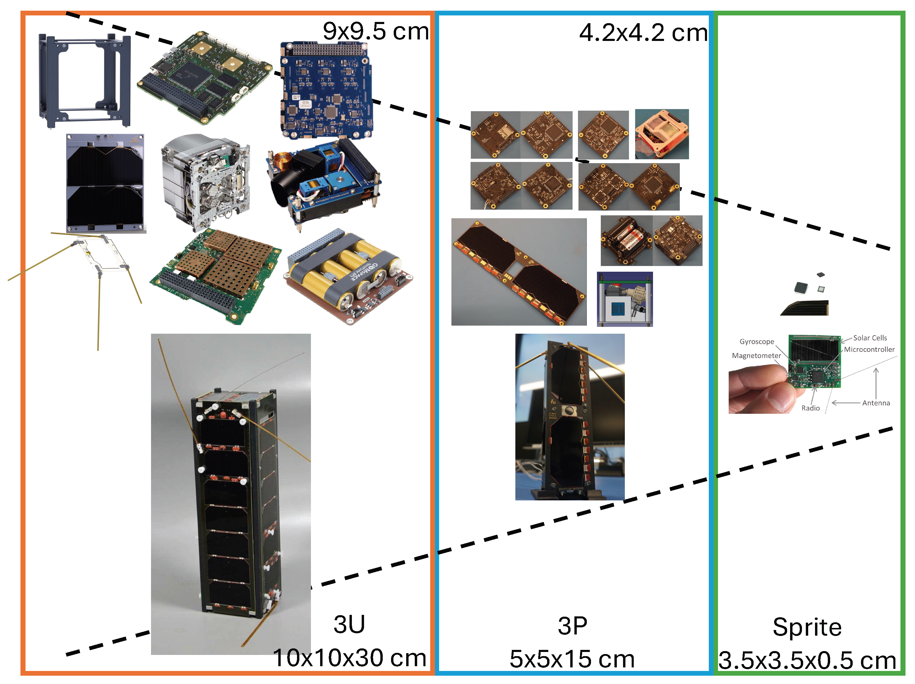
Figure 2.
Visualization of Contingency&Margin Terminology and how they add up. Adapted from [24].
Figure 2.
Visualization of Contingency&Margin Terminology and how they add up. Adapted from [24].
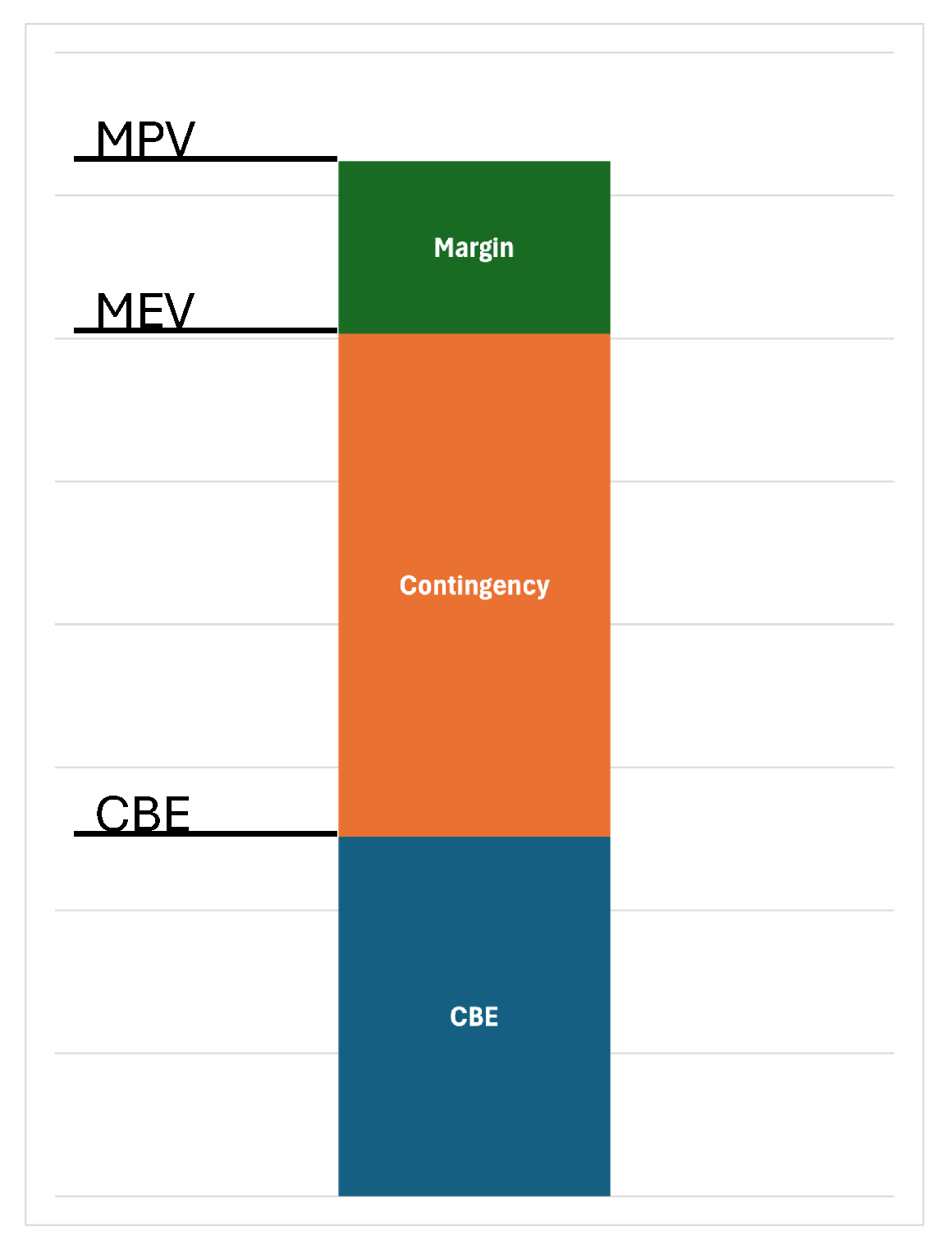
Figure 3.
Trends in power level categories for satellites, showing original AIAA categories [28] (green), extended bins (blue), and geometric averages (black/red dashed–lines) used for extrapolation. Lower end of the graph is shown as 0.1W instead of 0 due to logarithmic scale. Categories are respective power ranges for demonstration purposes.
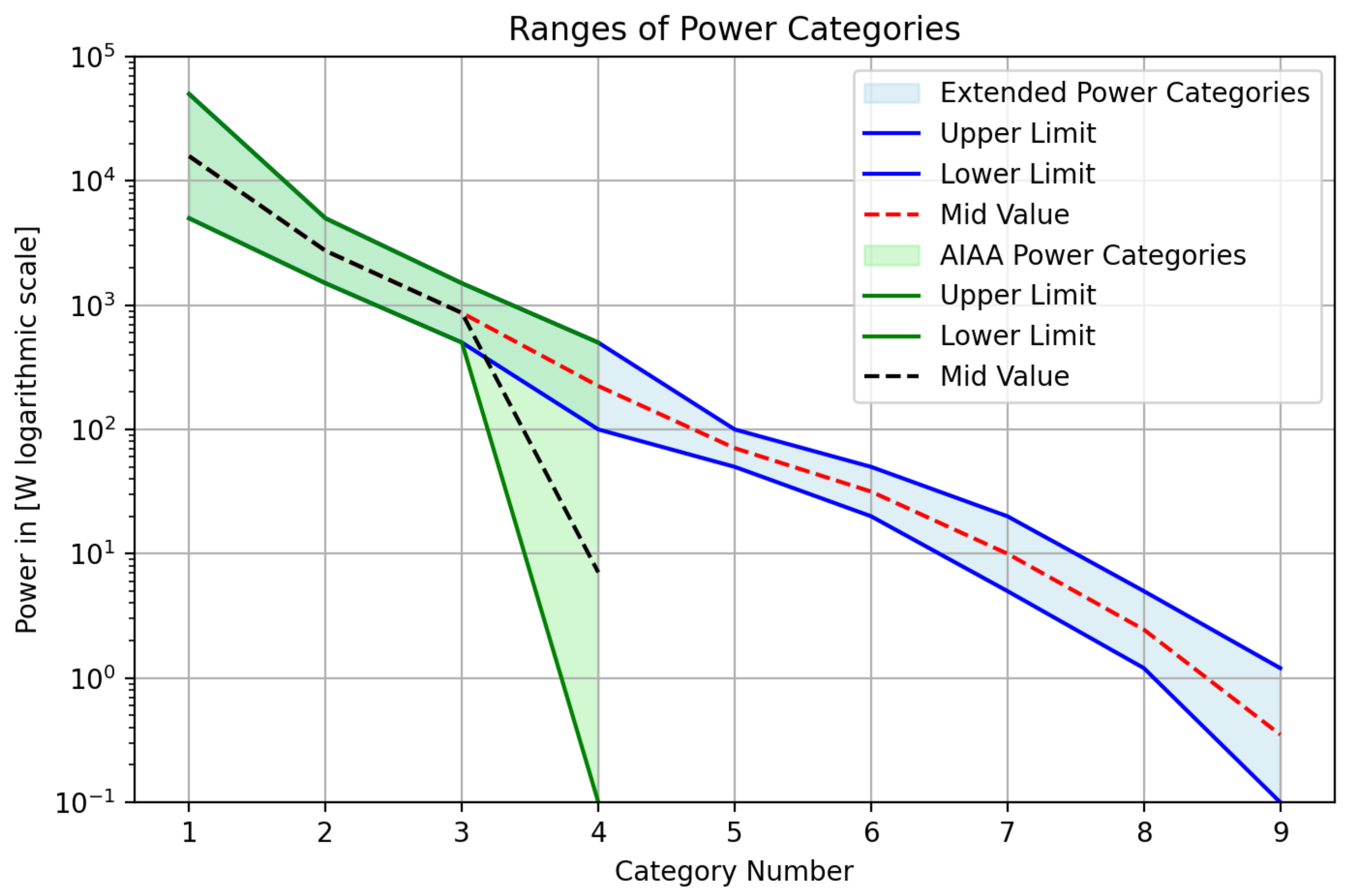
Figure 5.
Evolution of required power system sizing for the hypothetical Sprite Project, illustrating the reduction in MEV from (PDR, Sprite V1) to (CDR, Sprite V2) as design maturity and mission heritage increase. The numbers on each column represent the MEV.
Figure 5.
Evolution of required power system sizing for the hypothetical Sprite Project, illustrating the reduction in MEV from (PDR, Sprite V1) to (CDR, Sprite V2) as design maturity and mission heritage increase. The numbers on each column represent the MEV.
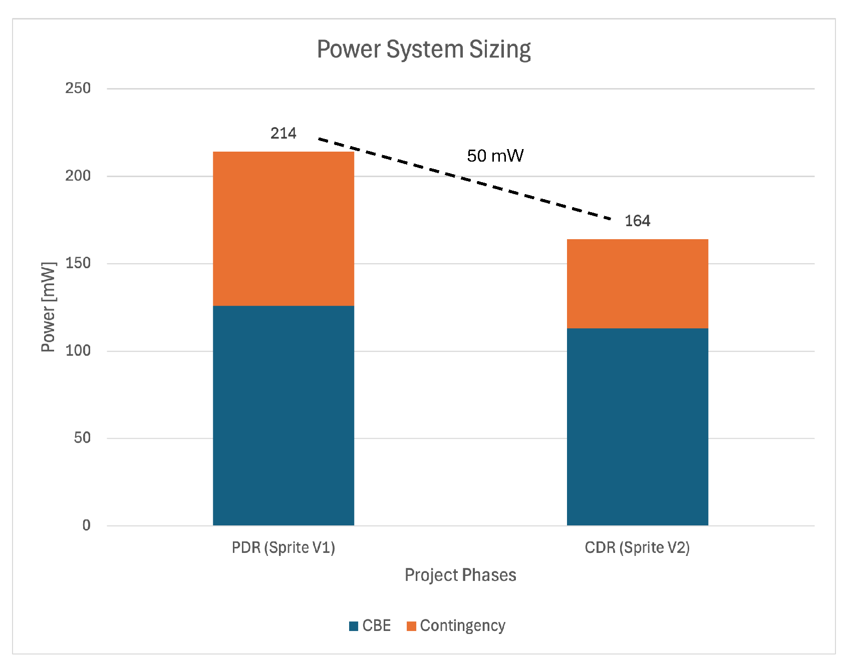
Figure 6.
Basic architecture of PlanarSats. Colors represent; PCB, solar cells and IC

Figure 7.
Solar panel sizing and operational power envelopes for PlanarSat architectures. (a) Cumulative power sizing from CBE(125.7mW) to MEV(301.68mW) to MPV(362.02mW). (b–d) Operational envelopes for separated, mixed, and half-mixed designs sized to MEV; (e–g) same designs sized to MPV. The maximum operational angle (angle of incidence) () is shown for each case.
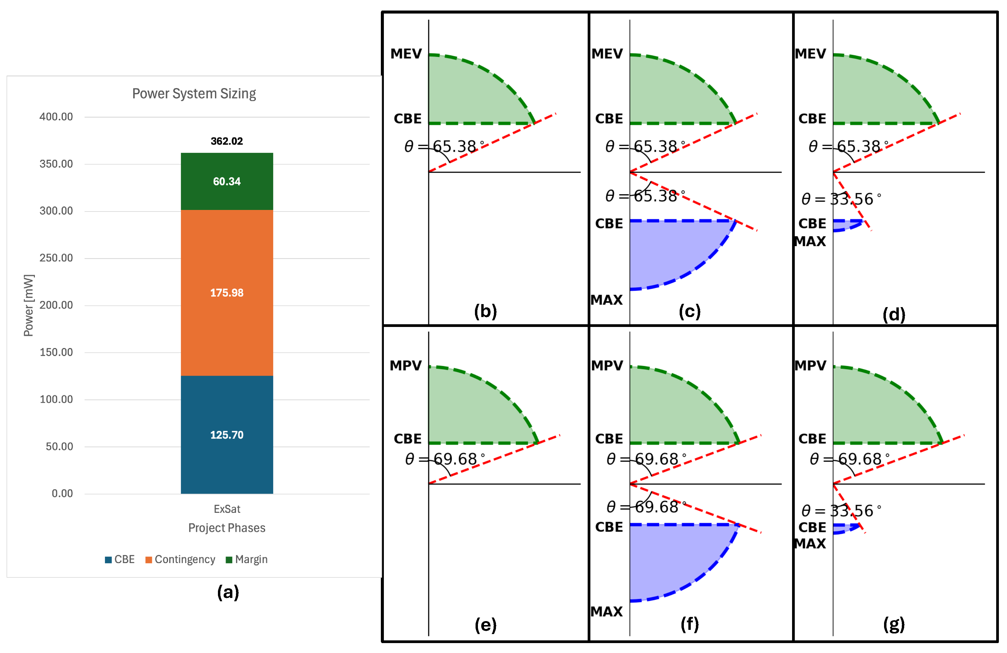
Table 5.
Standardized small satellites equipped with the maximum number of standard solar cells [40] on their X, Y, and Z surfaces. Power generation is calculated for a 45° angle on three surfaces.
Table 5.
Standardized small satellites equipped with the maximum number of standard solar cells [40] on their X, Y, and Z surfaces. Power generation is calculated for a 45° angle on three surfaces.
| Number of Cells on Surfaces |
Maximum Power at 45 degrees |
|||
|---|---|---|---|---|
| X | Y | Z | Total [W] | |
| 16U | 20 | 20 | 8 | 40.73 |
| 12U | 14 | 14 | 8 | 30.55 |
| 8U | 20 | 10 | 4 | 28.85 |
| 6U | 14 | 7 | 4 | 21.21 |
| 4U | 10 | 10 | 2 | 18.67 |
| 3U | 7 | 7 | 2 | 13.58 |
| 2U | 4 | 4 | 2 | 8.49 |
| 1U | 2 | 2 | 2 | 5.09 |
| 3P | 2 | 2 | 0.5 | 3.82 |
| 2P | 1.5 | 1.5 | 0.5 | 2.97 |
| 1.5P | 1 | 1 | 0.5 | 2.12 |
| 1P | 0.5 | 0.5 | 0.5 | 1.27 |
| 0.5P | 0.25 | 0.25 | 0.5 | 0.85 |
Table 6.
Extended Recommended Power Contingencies based on AIAA contingencies (minimum standard power reserve percentages) [28]. Original anchor values are maintained; extrapolated values are shown in italic. “Bid” corresponds to Proposal phase bid estimates; CoDR to Concept Design Review; PDR to Preliminary Design Review; CDR to Critical Design Review; and PRR to Production/Flight Readiness Review. Mission Class 1 represents the most conservative (high-reliability or low-maturity) case, while Class 3 represents the most aggressive (lower reliability or well-understood) case. All values are calculated and interpolated in log-space, with final recommendations rounded to the nearest integer for engineering use; parentheses indicate pre-rounded values. This approach ensures clarity and practical applicability in design calculations.
| Proposal Stage | Design Development Stage | |||||||||||||||||
|---|---|---|---|---|---|---|---|---|---|---|---|---|---|---|---|---|---|---|
| Bid | CoDR | PDR | CDR | PRR/FRR | ||||||||||||||
| Class | Class | Class | Class | Class | ||||||||||||||
|
Description/ Categories |
I | II | III | I | II | III | I | II | III | I | II | III | I-II-III | |||||
| 0-1.2W | 140 (137.78) |
65 (63.89) |
13 | 125 (122.78) |
40 (39.34) |
12 | 70 (68.89) |
45 (43.89) |
9 | 45 (43.89) |
40 (38.89) |
7 | 5 | |||||
| 1.2-5W | 125 (123.34) |
55 (56.67) |
13 | 110 (108.34) |
35 (35.00) |
12 | 60 (61.67) |
40 (36.67) |
9 | 40 (36.67) |
30 (31.67) |
7 | 5 | |||||
| 5-20W | 115 (112.95) |
55 (51.47) |
13 | 100 (97.95) |
30 (31.88) |
12 | 55 (56.47) |
30 (31.47) |
9 | 30 (31.47) |
25 (26.47) |
7 | 5 | |||||
| 20-50W | 100 (98.50) |
50 (47.22) |
13 | 90 (89.45) |
30 (29.33) |
12 | 55 (52.22) |
30 (27.22) |
9 | 30 (27.22) |
25 (22.22) |
7 | 5 | |||||
| 50-100W | 100 (98.50) |
45 (44.25) |
13 | 85 (83.50) |
30 (27.55) |
12 | 50 (49.25) |
25 (24.25) |
9 | 25 (24.25) |
20 (19.25) |
7 | 5 | |||||
| 100-500W | 90 | 40 | 13 | 75 | 25 | 12 | 45 | 20 | 9 | 20 | 15 | 7 | 5 | |||||
| 500-1500W | 80 | 35 | 13 | 65 | 22 | 12 | 40 | 15 | 9 | 15 | 10 | 7 | 5 | |||||
| 1500-5000W | 70 | 30 | 13 | 60 | 20 | 12 | 30 | 15 | 9 | 15 | 10 | 7 | 5 | |||||
| 5000W + | 40 | 25 | 13 | 35 | 20 | 11 | 20 | 15 | 9 | 10 | 7 | 7 | 5 | |||||
Table 7.
Summary of Analyzed Satellites: mission phases and classes, CBE, and calculated MEV
| Satellite | Mission Class | Design Phase | CBE (mW) | Contingency (%) | MEV (mW) | Notes |
|---|---|---|---|---|---|---|
| Sprite V1 | Class 1 | CDR | 126 | 45 | 182 | First of kind |
| Sprite V2 | Class 2 | CDR | 114 | 40 | 159 | Heritage from V1 |
| PCBSAT | Class 1 | CoDR | 746 | 125 | 1678 | First of kind |
| SpaceChip | Class 1 | Bid | 1.14 | 140 | 2.74 | New Concept |
| LuxAtto P | Class 2 | PDR | 462 | 45 | 669 | Predecessor Sprite |
| LuxAtto A&B | Class 1 | PDR | 70 (each) | 45 | 101.5 | New Form Factor |
Table 8.
Analyzed Satellites: power generation and solar cell characteristics [52,53,54,55,60]. Solar cells on Sprite V1 are presented in [61], on Sprite V2 are presented in [62], on Lux-P,A and B are [63]. PCBSat uses COTS cells and specifications from [52]. SpaceChip recommends a technology, specifications from [53].
| Specification / Satellite | Sprite V1 | Sprite V2 | PCBSat | SpaceChip | Lux-P | Lux-A&B |
|---|---|---|---|---|---|---|
| Power and Sizing | ||||||
| Power Requirement [mW] | 126 | 114 | 746 | 1.14 | 462 | 70 |
| Total Solar Cell Area [cm2] | 4.55 | 2.6 | 56 | 2.28 | 7.36 | 3.68 |
| Max Power Generation [mW] | 123 | 68 | 1131 | 1.87 | 105.2 | 52.6 |
| Solar Sized for Power [mW] | N/A | N/A | 821 (@45o) | 1.34 (@45o) | N/A | N/A |
| Satellite Dimensions [cm×cm] | 3.5×3.5 | 3.5×3.5 | 9×9.5 | 2×2 | 5×2.5 | 2.5×2.5 |
| Solar Cell Characteristics | ||||||
| Cell Efficiency [%] | 27 | 28 | 15 | 1 | 25 | 25 |
| [mA] | 28 | 14.6 | 250–275 | N/A | 5.9 | 5.9 |
| [V] | 2.19 | 2.33 | 0.484 | N/A | 4.46 | 4.46 |
| [mW] | 61.5 | 34 | 127 | N/A | 26.3 | 26.3 |
| Cell Area [cm2] | 2.277 | 1.3 | 8 | N/A | 1.84 | 1.84 |
| Power Density [mW/cm2] | 27 | 26.15 | 15.88 | N/A | 14.3 | 14.3 |
| Cell Technology | Triple-J GaAs | Triple-J GaAs | Silicon | N/A | Silicon | Silicon |
Disclaimer/Publisher’s Note: The statements, opinions and data contained in all publications are solely those of the individual author(s) and contributor(s) and not of MDPI and/or the editor(s). MDPI and/or the editor(s) disclaim responsibility for any injury to people or property resulting from any ideas, methods, instructions or products referred to in the content. |
© 2025 by the authors. Licensee MDPI, Basel, Switzerland. This article is an open access article distributed under the terms and conditions of the Creative Commons Attribution (CC BY) license (http://creativecommons.org/licenses/by/4.0/).
Copyright: This open access article is published under a Creative Commons CC BY 4.0 license, which permit the free download, distribution, and reuse, provided that the author and preprint are cited in any reuse.


