
Submitted:
26 June 2025
Posted:
27 June 2025
You are already at the latest version
Abstract
Semantic segmentation of 3D LiDAR point clouds is crucial for autonomous driving and urban modeling, but requires extensive labeled data. Unsupervised domain adaptation from synthetic to real data offers a promising solution, yet faces the challenge of negative transfer, particularly due to context shifts between domains. This paper introduces Context-Aware Feature Adaptation, a novel approach to mitigate negative transfer in 3D unsupervised domain adaptation. The proposed approach disentangles object-specific and context-specific features, refines source context features through cross-attention with target information, and adaptively fuses the results. We evaluate our approach on challenging synthetic-to-real adaptation scenarios, demonstrating consistent improvements over state-of-the-art domain adaptation methods with up to 7.9% improvement in classes subject to context shift. Our comprehensive domain shift analysis reveals a positive correlation between context shift magnitude and performance improvement. Extensive ablation studies and visualizations further validate the efficacy in handling context shift for 3D semantic segmentation.
Keywords:
UDA
; 3D point clouds
; domain shift
; 3D semantic segmentation
; negative transfer
1. Introduction
Semantic segmentation of outdoor mobile mapping point clouds is vital for applications like autonomous driving and digital twins of cities. Supervised deep learning methods achieve strong results but rely on large annotated datasets, which are costly and time-consuming to obtain. This has led to exploring transfer learning from synthetic datasets with readily available labels [1,2]. However, the domain shift between synthetic and real data introduces challenges, including sensor variations, geographical differences, and class discrepancies in urban scenes, causing a generalization gap in real-world scenarios. Unsupervised Domain Adaptation (UDA) methods have been proposed to address this gap [3,4,5,6,7]. Despite progress, UDA methods face challenges like negative transfer (NT), where irrelevant information from the source domain degrades target domain performance [8]. NT arises from cross-domain context shifts, such as spatial and co-occurrence changes between classes. For instance, in synthetic datasets, motorcycles may appear on roads, while in real-world data, they might be parked on sidewalks or terrain, causing class confusion. UDA methods for 3D semantic segmentation are commonly divided into self-training and adversarial. Self-training approaches may suffer from error propagation [9], while adversarial methods can misalign features, losing domain-specific context [10]. Current UDA efforts primarily focus on cross-domain transferability, often transferring domain-specific features from the source to the target, exacerbating NT [8]. This paper proposes Context-Aware Feature Adaptation (CAFA) to tackle NT caused by context shifts in 3D UDA. CAFA selectively adapts context-specific features while preserving domain-invariant object features. CAFA’s three-step process first disentangles object and context features, refines source context features using target context via cross-attention, and fuses refined context features with object features. Our contributions are:
- A novel feature disentanglement technique for separating object-specific and context-specific information in 3D point cloud data and a cross-attention mechanism for refining source context features using target domain information.
- A flexible framework integrating various UDA techniques to enhance performance.
- A method to quantify context shift to enable an analytical evaluation of performance improvements relative to context variability.
- Extensive experiments demonstrating our approach reduces NT and improves UDA performance on challenging 3D semantic segmentation tasks.
2. Related Work
Unsupervised domain adaptation for 3D semantic segmentation. UDA for 3D semantic segmentation enables knowledge transfer from labeled synthetic data to unlabeled real-world LiDAR scans. The key challenge is context shift due to different class co-occurrences between domains. Existing methods fall into adversarial [2,4,7,11,12,13,14,15,16] and self-training methods [3,5,6]. CycleGAN [17] can be used for translating real Bird-Eye-View images (BEV) into synthetic BEVs obtained from synthetic point clouds [11]. Zhao et al. [12] adversarially simulate LiDAR dropout noise on real data using a synthetic dataset. Xiao et al. [2] decompose the synthetic-to-real gap into an appearance component and a sparsity component and then align the synthetic and real feature distribution at the input level and feature level. Yi et al. [13] propose to conduct UDA through the auxiliary task of 3D surface completion to transfer knowledge between different LiDAR sensors. Yuan et al. [4] propose a category-level adversarial alignment to translate point density between domains with an adaptive adversarial loss reweighting and source-aware consistency loss. Li et al. [14] simulate the pattern of target noise to bridge the domain gap using a learnable masking module. Self-training methods use target pseudo-labels to bridge the domain gap. Saltori et al. [3] propose a self-training approach that employs a semantic mixing strategy to augment the data and mitigate domain shift. Xiao et al. [6] introduce LiDAR-specific augmentation through scene-level swapping and instance-level rotation. Zhao et al. [5] construct a bridge domain through spatial, intensity, and semantic distribution mixing. While some approaches tackle aspects of NT [7,14], they do not explicitly address context shifts due to varying class co-occurrences. Current methods struggle to capture differing contextual relationships between domains, leading to suboptimal feature transfer in complex urban environments. Our proposed method addresses this gap with a novel context-aware feature disentanglement approach and cross-attention refinement, specifically designed to handle spatial dependencies and class co-occurrence variations to mitigate NT caused by context shifts in 3D LiDAR segmentation.
Negative Transfer in UDA. The effectiveness of UDA methods can be compromised by NT, where knowledge from the source domain harms target performance. NT often occurs when domains are dissimilar [18] or when source models overfit to domain-specific features. This is problematic in outdoor mobile mapping point clouds, where context shifts between domains can occur due to complex spatial relationships, class co-occurrences, and varying point densities across different environments. NT mitigation approaches can be categorized into two main categories [8]: data transferability enhancement (DTE) and model transferability enhancement (MTE). DTE methods focus on enhancing the quality of input instances or features. These include domain decomposition [19,20], which performs UDA on subdomains by partitioning the source and target into different parts. For instance, Zhu et al. [19] minimize class-wise discrepancy rather than global alignment. Intermediate domain construction methods [21,22] bridge the domain gap through constructed intermediate domains. Other DTE approaches include instance selection and weighting [23], and feature enhancement methods such as batch spectral shrinkage [24] and adaptive channel weighting [25]. MTE approaches aim to enhance model transferability. These include TransNorm [25], which adapts normalization statistics, and parameter selection methods, such as TransPar [26], which identify and select transferable parameters from the source model. Parameter regularization methods, including co-tuning [27], side-tuning [28], and concept-wise fine-tuning [29], also fall under the MTE category. However, these methods must explicitly address context shift, a critical factor for 3D point clouds due to the varying scene compositions across different urban environments.
Our proposed method addresses the limitations of existing approaches in handling context shift by introducing a context-aware feature disentanglement approach coupled with cross-attention refinement. This allows for targeted adaptation of contextual features while preserving object-specific information.
3. Materials and Methods
Our proposed approach explicitly handles contextual differences during the adaptation process and is illustrated in Figure 1. We consider a set of source domain samples and target domain samples , are source input points and are target points. and denote source and target feature distributions respectively and is the number of input features. are source labels for C classes. and are the number of source and target points respectively. The target domain shares the same classes as the source domain; the target labels are unknown.
3.1. Context Aware Feature Adaptation
In the following sections, we detail each component of our proposed Context Aware Feature Adaptation (CAFA) method.
3.1.1. Object and Context Feature Disentanglement
We decompose source and target features into object-specific and context-specific components to adapt contextual information while preserving object-specific features. Features are extracted at two abstraction levels through the backbone network as shown in Equation 1:
where are source features at level l, is the number of levels, is the feature dimension, and is the number of source points at level l. This applies to both source and target domains. Source features are disentangled using two attention modules to generate context (Equation 2) and object attention maps (Equation 3) which modulate the features via element-wise multiplication to produce context-specific (Equation 4) and object-specific features (Equation 5).
g and o denote abstraction levels (), and are 1x1 convolutional layers, and is the Softmax function. Lower levels (g) capture low-level context patterns, while higher levels (o) encode abstract object information. Only context-specific features are extracted for the target domain to guide source context refinement.
This disentanglement process uses multi-scale features and attention for a soft separation, allowing shared information between object and context features. Unlike strict orthogonality constraints (ineffective in our experiments), our method allows for soft disentanglement that maintains some shared information between object and context features.
3.1.2. Source Context Feature Refinement
We use cross-attention to refine source context features using target domain information. The process involves three steps:
First, we compute the global target context (Equation 6) using Global Average Pooling. Next, we compute a query context vector using a 1x1 convolutional layer A (Equation 7) that is then used to calculate attention weights for the source context features (Equation 8). Finally, we refine source context features using these attention weights through element-wise multiplication (Equation 9). This mechanism allows the model to selectively focus on source context features relevant to the target domain, and mitigate context shift effects.
3.1.3. Cross-Domain Feature Fusion
We fuse the refined source context features with the original source object features following Equation 10:
is a learnable 1x1 convolutional layer and denotes channel-wise concatenation. A residual connection with a learnable scalar (initialized small) allows the network to retain information from the original representation and adjust its importance during training. This process aligns source context features with the target domain while preserving important object-specific information for segmentation.
Algorithm 1 synthesizes the main steps of the proposed approach.
| Algorithm 1 Context-Aware Feature Adaptation (CAFA) |
|
3.2. Relationship to Other Attention Mechanisms
3.2.1. Vector Attention
Vector self attention was introduced in Point Transformer [30] for a set of feature vectors as :
is the output feature. , , and are pointwise feature transformations, such as multilayer perceptrons (MLPs) or linear projections. is a positional encoding function and is a mapping function (e.g., an MLP) that produces attention vectors for feature aggregation. The overall mechanism computes a vector-valued weighted sum and allows each channel in to selectively aggregate information from its neighbours as shown in Figure 2(b). In the proposed feature disentanglement module, each point features are re-calibrated independently based solely on its own representation—essentially performing a self-modulation akin to squeeze-and-excitation [31], without explicitly aggregating information from neighbouring points. This process is illustrated in Figure 2(c).
3.2.2. Squeeze-and-Excitation Module
The Squeeze and Excitation module [31] performs global average pooling to squeeze the spatial dimension. The resulting vector is then fed through an MLP and a sigmoid function to produce channel-wise weights which are applied for all spatial positions (Figure 2(a)). In our proposed source context feature refinement module, the spatial dimension is squeezed but further used to compute point-wise attention vectors for each target domain position.
3.3. Training Objective
Our method enhances existing UDA techniques by addressing NT and can integrate with various UDA methods to improve performance. The overall training objective (Equation 13) includes the cross-entropy loss on source data (Equation 12) and a UDA-specific loss , which depends on the chosen UDA method (e.g., adversarial loss, self-training loss, or other domain alignment objectives):
h is the classifier computed on the refined source features.
4. Results
4.1. Datasets and Baselines
4.1.1. Datasets
We evaluate our method in a synthetic-to-real UDA setting, training on synthetic data and adapting to real-world datasets. We align our validation split and training setup with previous works [2,3]. The SynLiDAR dataset [2], created with Unreal Engine and a simulated 64-beam LiDAR, serves as the source domain. We use SemanticPOSS [32] and SemanticKITTI [33] for target domains. Labels are aligned into common sets: 13 classes for SynLiDAR to SemanticPOSS and 19 for SynLiDAR to SemanticKITTI [2,3]. Segmentation performance is measured using mean Intersection over Union (mIoU) [34].
4.1.2. Baselines and Training.
We compare our method against state-of-the-art 3D UDA methods and NT mitigation techniques. For 3D UDA, we use PCAN [4], a density-guided adversarial method and CoSMix [3], a self-training approach with cross-domain semantic mixing. To assess NT mitigation, we use DSAN [19], CWFT [29], TransPar [26], and BSS [24] with each UDA method. We use MinkUNet32 [35] as the backbone for point cloud semantic segmentation. The input voxel size is set to 0.05 m, and the implementation is in PyTorch using a single NVIDIA Tesla V100 GPU. We pretrain on the source domain for ten epochs using SGD (learning rate 0.01, momentum 0.9, batch size 4), this pretrained model serves as the baseline. We initialize with pre-trained weights during adaptation and follow each baseline’s original implementation and hyperparameters for a fair comparison. Our method sets the context abstraction level to (first network layer), and object-specific features o are from the last layer before classification. All attention modules use 1x1 sparse convolution layers. We provide below more details about the hyperparameters used for adaptation and training all the negative transfer methods for both PCAN [4] (Table 1) and CosMix [3] (Table 2).
4.2. Feature Disentanglement Results
The object and context attention maps generated by our CAFA method are illustrated in Figure 3. As described in Section 3.1.1, these attention maps are computed at different abstraction levels within the network and confirm that the model learns a meaningful separation of object and context features. In Figure 3, object attention maps indicate points that the model deems most important for discriminating objects such as parts of cars and buildings and urban objects on sidewalks. On the other hand, context attention maps highlight points that provide contextual cues, such as the surroundings that help the model interpret the object in its setting (e.g. ground, cars, buildings, or other spatial context).
4.3. Comparison with Previous Methods
We evaluate CAFA on two challenging UDA scenarios: SynLiDAR → SemanticKITTI (Table 3) and SynLiDAR → SemanticPOSS (Table 4). We report the results in terms of mean Intersection over the Union (mIoU).
Overall Performance: CAFA consistently outperforms baseline UDA methods in both adaptation scenarios. In SynLiDAR → SemanticKITTI, it improves CoSMix by 1.6 mIoU to 34.5%, with notable gains in "motorcycle" (+7.6%), "bicyclist" (+7.9%), and "terrain" (+6.7%), though slight decreases in "car" (-0.4%) and "building" (-2.5%). Applied to PCAN, CAFA improves mIoU by 0.4 points, with gains in "motorcycle" (+4.3%) and "bicyclist" (+7.5%), but drops in "traffic sign" (-5.6%). In SynLiDAR to SemanticPOSS (Table 4), CAFA shows consistent improvements. Integrated with CoSMix, it gains 1.0 mIoU to reach 45.0%, improving "car" (+9.3%) and "pole" (+1.4%), though decreases in "person" (-3.0%) and "traffic" (-2.7%). Applied to PCAN, CAFA adds 0.9 mIoU, with gains in "rider" (+1.7%) and "building" (+1.2%), but drops in "traffic" (-0.3%) and "bike" (-1.6%).
Comparison with Negative Transfer Mitigation Methods: CAFA outperforms all other mitigation methods when applied to CoSMix on SynLiDAR → SemanticKITTI, achieving 34.5% mIoU versus 33.4% for the next best (DSAN). Some techniques (CWFT, GCR, TransPar, BSS) reduce CoSMix’s performance, highlighting challenges in mitigating negative transfer in 3D segmentation. For PCAN on SemanticKITTI, improvements are smaller; CAFA and TransPar achieve the highest mIoU (37.3%), suggesting PCAN may be more robust, but CAFA still provides benefits. In SynLiDAR to SemanticPOSS, CAFA again leads when applied to CoSMix, achieving 45.0% mIoU compared to 44.3% for BSS. Applied to PCAN, CAFA reaches the highest mIoU (45.5%), with TransPar close at 44.9%. These results demonstrate that CAFA consistently outperforms other negative transfer mitigation techniques across UDA methods and datasets.
4.4. Qualitative Analysis
We further illustrate how CAFA leverages target context by comparing segmentation outputs with baseline approaches. Figure 4 and Figure 5 illustrate qualitative segmentation results for SynLiDAR→SemanticPOSS and SynLiDAR→SemanticKITTI adaptations respectively, comparing ground truth labels with predictions from CoSMix and our CAFA method.
In Figure 4, classes such as buildings and fence show improved performance. Confusion arises in these classes due to contextual similarities with other semantic categories. For instance, buildings are frequently misclassified as vegetation, and fences are often mislabelled as vegetation or cars. This is due to the higher co-occurrence of buildings with vegetation and vegetation with tree trunks in SemanticPOSS. Consequently, a model might learn a misleading association linking vegetation to trunks and at test time it may mislabel facade points as vegetation if trunk points are nearby. Cars co-occur with vegetation and ground often in SynLiDAR. When a context shift makes the model wrongly spot vegetation around a fence in SemanticPOSS, that same association can cause fences to be mislabelled as cars. After CAFA, car, which is one of the classes showing the most context shift in SemanticPOSS, shows less confusion with fences.
In Figure 5, CAFA effectively distinguishes between the classes terrain, sidewalk, and other-ground, despite their frequent co-occurrence in SynLiDAR. Specifically, the high proximity of other-ground to roads in SynLiDAR creates a spurious correlation, prompting simultaneous predictions for these classes. After applying CAFA, the erroneous prediction of other-ground is significantly reduced, which reflects its weaker association with the other surfaces in SemanticKITTI. Figure 5 (i) demonstrates CAFA’s capability to distinguish trunk from person, a class affected by context shift. In SynLiDAR, person frequently co-occurs with sidewalks, creating a strong correlation that causes confusion when sidewalks are predicted nearby. CAFA mitigates this issue, resolving such misclassifications even when sidewalks are still predicted in its neighbourhood.
Figure 6(b) illustrates the effectiveness of CAFA in handling context shifts. CAFA correctly identifies the sidewalk beneath parked cars, a common scenario in the target domain but not the source, while CoSMix misclassifies it as road. To understand this improvement, we visualize the points contributing most to the class prediction using GradCAM [36]. CoSMix’s attention map (Figure 6(e)) shows that when predicting road, it focuses on a wide range of elements, including the cars themselves and buildings. In contrast, CAFA’s attention map (Figure 6(d)) demonstrates a more refined focus. When classifying the same area, CAFA concentrates on the cars and nearby urban objects commonly found on sidewalks. This targeted attention indicates that CAFA has learned to associate these specific elements with sidewalks in the target domain.
4.5. Ablation Study
To evaluate each component of our design, we conducted ablation studies aimed at clarifying the impact of our specific architectural choices on SynLiDAR → SemanticPOSS. Specifically, we explored five key modifications:
Single-scale vs. Multi-scale Features: We investigated whether using single-scale features for both object and context representations is sufficient, compared to our original multi-scale design.
Impact of different context representation: To determine whether performance gains result primarily from integrating additional contextual information, we compared our approach to a baseline employing single-domain self-attention for both source and target. We also benchmarked our context modeling against the Global Context Reasoning (GCR) module proposed by Ma et al. [37], which leverages channel similarity to construct graph nodes that are processed by Graph Convolutional Networks (GCN).
Use of object features alone: To isolate the contribution of context alignment, we assessed performance when classification relied solely on object features.
Fusion Strategy Evaluation: Finally, we evaluated the effectiveness of our fusion approach by comparing it against a simpler alternative using direct summation of object and context representations. We also analyze the impact of using a residual connection for gradual adaptation.
We summarize the results of our ablation studies in Table 5.
Multi-scale Feature Disentanglement: Using single-scale features results in a 0.9 mIoU drop, confirming that multi-scale features capture richer contextual and object-specific information.
Cross-attention: Cross-domain context transfer outperforms single-domain context modeling. Self-attention on source and target features decreases mIoU by 0.8% and 1.3%, respectively, and the GCR module [37] also reduces performance, emphasizing the necessity of cross-attention to address context shift.
Feature Fusion: Replacing adaptive fusion with simple summation reduces performance by 0.7 mIoU.
Context Features: Using only object features for classification decreases performance, which highlights the value of integrating both context and object-specific features.
Residual Connection: Removing the residual connection in feature fusion caused a -2.8 mIoU drop, showing its role in preserving original representations while gradually introducing target context features.
4.6. Context Shift Performance Analysis
To evaluate CAFA’s efficacy in addressing context shift, we analyzed class-wise performance improvements relative to context shift, quantified by the L1 distance between class co-occurrence matrices of the source and target domains. Using balanced sampling ( points per cloud), we computed neighborhood class statistics to create normalized co-occurrence matrices. We sample points from each domain and look at their neighborhood to determine how often each class co-occurs with every other class. The frequency of these pairwise co-occurrences is then normalized and arranged into a matrix. A high value in , means appears frequently near . Figure 7 and Figure 8 shows differences between source and target domains. For instance, SynLiDAR shows weaker co-occurence between vehicles and drivable surfaces and classes such as car or person have lower co-occurrence with environmental classes like building, vegetation, or sidewalk compared to SemanticKITTI (Figure 8(b)). In SemanticPOSS, cars appear alongside environmental labels more often than in SynLiDAR (Figure 7(b)).
The L1 distance provides a measure of context shift for each class, defined as the absolute difference between its class occurrence distributions in the source and target domains. Specifically, it corresponds to the sum of absolute differences between the rows representing class occurrences in the co-occurence matrices, where each row characterizes a specific class’s occurence with other classes. We plot context shift against performance improvement for CoSMix and PCAN on SemanticKITTI and SemanticPOSS (Figure 9). Results show a positive correlation: classes with more significant shifts exhibit greater performance gains, as indicated by CAFA’s trend line (green), which consistently slopes positively. In contrast, the best-performing NT method (purple) occasionally exhibits negative slopes, highlighting CAFA’s ability to mitigate NT for high-shift classes. To validate further, we computed mean mIoU for the top three high-shift classes in PCAN and CoSMix across UDA tasks (Table 6). CAFA consistently outperforms other methods, achieving a 5.8 mIoU improvement on average compared to 1.4 for the best NT approach.
To further illustrate how context shift affects adaptation, we highlight in Table 6 the top three classes in each scenario with the largest co-occurrence mismatch, i.e. the greatest context shift, across both PCAN and CoSMix on SynLiDAR → SemanticKITTI and SynLiDAR → SemanticPOSS adaptations. Compared to both the baseline UDA methods (PCAN, CoSMix) and other negative transfer mitigation approaches, CAFA consistently yields larger mIoU gains for these high-shift classes. For SynLiDAR → SemanticKITTI, CAFA achieves a gain of +4.4% in mIoU compared to +0.9% for the best-performing NT method with PCAN. Similarly, for CoSMix, CAFA achieves a gain of +6.2% compared to +3.8% for NT. For SynLiDAR → SemanticPOSS, CAFA achieves a gain of +10.6% in mIoU compared to +0.1% for the best-performing NT method with PCAN. For CoSMix, CAFA achieves a gain of +2.0% compared to +1.0% for NT.
This analysis illustrates that targeting negative transfer due to context shift, is an effective way to mitigate performance drops that occur when knowledge from the source domain is not directly applicable in the target domain.
5. Discussion
The first component of CAFA is its ability to disentangle object-specific and context-specific features. This separation is achieved through attention mechanisms at different abstraction levels as opposed to rigid approaches that enforce strict orthogonality between features. This soft disentanglement preserves useful shared information and allows for the selective adaptation of source context features using the target domain. It also prevents the transfer of misleading contextual biases and is supported by the performance improvements observed in our ablation studies and context shift analysis.
To mitigate context shift, it’s crucial to have a method to quantify it and evaluate performance improvements relative to context variability. Our quantitative analysis using normalized class co-occurrence matrices to measure context shift shows a positive correlation between the magnitude of context shift and segmentation performance gains. For example, as shown in Figure 9 and Table 6, classes with high context shifts exhibit significant improvements in mIoU when CAFA is applied. These results confirm our working hypothesis: when the degree of context mismatch between source and target domains is large, incorporating target domain context into the adaptation process is particularly beneficial. Our findings indicate that CAFA outperforms other mitigation strategies (e.g., DSAN, CWFT, TransPar, BSS) by delivering higher mIoU gains, particularly for classes with significant context mismatches.
From a practical standpoint, mitigating negative transfer in applications such as autonomous driving, urban mapping, and robotics is essential for developing robust real-world systems. This enables segmentation models to generalize better across varied urban environments—where the spatial relationships between objects may differ significantly between the training and deployment domains. The demonstrated positive correlation between context shift and performance improvement provides a quantitative basis for future evaluation metrics and shows the importance of integrating context in UDA for semantic segmentation .
6. Conclusions
Our proposed method addresses negative transfer in unsupervised domain adaptation for 3D LiDAR semantic segmentation. Disentangling object-specific and context-specific features and refining source context features using target domain information effectively mitigates the impact of context shift between domains. Our domain shift analysis, quantifying the relationship between class-wise performance improvements and the degree of shift for each class, provides strong evidence for its effectiveness. Furthermore, experimental results on challenging synthetic-to-real adaptation scenarios consistently show performance improvements over state-of-the-art UDA methods and existing negative transfer mitigation techniques.
However, our approach has some limitations. The proposed feature disentanglement relies on a simple attention mechanism, which may only partially model complex contextual relationships in some scenarios. Additionally, the method assumes a closed-set adaptation setting, which can limit its applicability in real-world scenarios where new classes may appear in the target domain. Future work could explore more sophisticated feature disentanglement techniques to improve object and context information separation. Finally, extending the method to handle open-set and partial-domain adaptation scenarios would also increase its practical utility.
Author Contributions
Conceptualization, L.E., S.D. and T.B; methodology, L.E., S.D. ; software,L.E.; validation, L.E., S.D. and T.B.; formal analysis, L.E., S.D.; investigation, L.E.; resources, S.D.; data curation, L.E.; writing—original draft preparation, L.E.; writing—review and editing, L.E., S.D. and T.B.; visualization, L.E.; supervision, S.D. and T.B.; project administration, S.D.; funding acquisition, S.D.; All authors have read and agreed to the published version of the manuscript.
Funding
This research was funded by MITACS Accelerate program (Grant Number IT19956) and the Natural Sciences and Engineering Research Council (NSERC) of Canada (Grant Number RGPIN-2018-04046).
Data Availability Statement
The SemanticKITTI dataset’s official website is www.semantic-kitti.org. The SemanticPOSS dataset’s official website is www.poss.pku.edu.cn/semanticposs.html. The SynLiDAR dataset’s official website is www.github.com/xiaoaoran/SynLiDAR.
Acknowledgments
The authors gratefully acknowledge the support of MITACS Accelerate program, the Natural Sciences and Engineering Research Council, the Research Center in Geospatial Data and Intelligence of Université Laval, the Institute on intelligence and Data of Université Laval and the Digital Research Alliance of Canada for access to their Advanced Research Computing platform and computational resources to complete our experiments.
Conflicts of Interest
The authors declare no conflicts of interest.
Abbreviations
The following abbreviations are used in this manuscript:
| UDA | Unsupervised Domain Adaptation |
| NT | Negative Transfer |
| MLP | Multilayer Perceptron |
| mIoU | mean Intersection over Union |
| BEV | Bird-Eye-View images |
| DTE | data transferability enhancement |
| MTE | model transferability enhancement |
| SE-Net | Squeeze-and-Excitation |
| SGD | Stochastic Gradient Descent |
References
- Wu, B.; Zhou, X.; Zhao, S.; Yue, X.; Keutzer, K. SqueezeSegV2: Improved Model Structure and Unsupervised Domain Adaptation for Road-Object Segmentation from a LiDAR Point Cloud. pp. 4376–4382.
- Xiao, A.; Huang, J.; Guan, D.; Zhan, F.; Lu, S. Transfer Learning from Synthetic to Real LiDAR Point Cloud for Semantic Segmentation. 36, 2795–2803. [CrossRef]
- Saltori, C.; Galasso, F.; Fiameni, G.; Sebe, N.; Poiesi, F.; Ricci, E. Compositional Semantic Mix for Domain Adaptation in Point Cloud Segmentation. IEEE Transactions on Pattern Analysis and Machine Intelligence 2023, 45, 14234–14247.
- Yuan, Z.; Zeng, W.; Su, Y.; Liu, W.; Cheng, M.; Guo, Y.; Wang, C. Density-guided Translator Boosts Synthetic-to-Real Unsupervised Domain Adaptive Segmentation of 3D Point Clouds. ArXiv 2024, abs/2403.18469.
- Zhao, H.; Zhang, J.; Chen, Z.; Zhao, S.; Tao, D. UniMix: Towards Domain Adaptive and Generalizable LiDAR Semantic Segmentation in Adverse Weather. ArXiv 2024, abs/2404.05145.
- Xiao, A.; Huang, J.; Guan, D.; Cui, K.; Lu, S.; Shao, L. PolarMix: A General Data Augmentation Technique for LiDAR Point Clouds. ArXiv 2022, abs/2208.00223.
- Yuan, Z.; Cheng, M.; Zeng, W.; Su, Y.; Liu, W.; Yu, S.; Wang, C. Prototype-Guided Multitask Adversarial Network for Cross-Domain LiDAR Point Clouds Semantic Segmentation. IEEE Transactions on Geoscience and Remote Sensing 2023, 61, 1–13.
- Zhang, W.; Deng, L.; Zhang, L.; Wu, D. A Survey on Negative Transfer. IEEE/CAA Journal of Automatica Sinica 2023, 10, 305–329. Conference Name: IEEE/CAA Journal of Automatica Sinica, . [CrossRef]
- Liang, J.; Wang, Y.; Hu, D.; He, R.; Feng, J. A Balanced and Uncertainty-aware Approach for Partial Domain Adaptation. In Proceedings of the European Conference on Computer Vision, 2020.
- Li, S.; Xie, M.; Lv, F.; Liu, C.H.; Liang, J.; Qin, C.; Li, W. Semantic Concentration for Domain Adaptation. 2021 IEEE/CVF International Conference on Computer Vision (ICCV) 2021, pp. 9082–9091.
- Saleh, K.; Abobakr, A.; Attia, M.; Iskander, J.; Nahavandi, D.; Hossny, M.; Nahvandi, S. Domain Adaptation for Vehicle Detection from Bird's Eye View LiDAR Point Cloud Data. In Proceedings of the 2019 IEEE/CVF Int. Conf. Comput. Vis. Workshops, ICCVW, pp. 3235–3242. [CrossRef]
- Zhao, S.; Wang, Y.; Li, B.; Wu, B.; Gao, Y.; Xu, P.; Darrell, T.; Keutzer, K. ePointDA: An End-to-End Simulation-to-Real Domain Adaptation Framework for LiDAR Point Cloud Segmentation. In Proceedings of the AAAI Conf. Artif. Intell., AAAI.
- Yi, L.; Gong, B.; Funkhouser, T. Complete & Label: A Domain Adaptation Approach to Semantic Segmentation of LiDAR Point Clouds. In Proceedings of the IEEE/CVF Conf. Comput. Vis. Pattern Recognit., CVPR, pp. 15358–15368. [CrossRef]
- Li, G.; Kang, G.; Wang, X.; Wei, Y.; Yang, Y. Adversarially Masking Synthetic to Mimic Real: Adaptive Noise Injection for Point Cloud Segmentation Adaptation. 2023 IEEE/CVF Conference on Computer Vision and Pattern Recognition (CVPR) 2023, pp. 20464–20474.
- Wang, Z.; Ding, S.; Li, Y.; Zhao, M.; Roychowdhury, S.; Wallin, A.; Sapiro, G.; Qiu, Q. Range Adaptation for 3D Object Detection in LiDAR. In Proceedings of the 2019 IEEE/CVF Int. Conf. Comput. Vis. Workshops, ICCVW, pp. 2320–2328. [CrossRef]
- Luo, H.; Khoshelham, K.; Fang, L.; Chen, C. Unsupervised scene adaptation for semantic segmentation of urban mobile laser scanning point clouds. 169, 253–267. [CrossRef]
- Zhu, J.Y.; Park, T.; Isola, P.; Efros, A.A. Unpaired Image-to-Image Translation Using Cycle-Consistent Adversarial Networks. In Proceedings of the 2017 IEEE/CVF Int. Conf. Comput. Vis., ICCV, pp. 2242–2251. [CrossRef]
- Rosenstein, M.T.; Marx, Z.; Kaelbling, L.P.; Dietterich, T.G. To transfer or not to transfer. In Proceedings of the Neural Information Processing Systems, 2005.
- Zhu, Y.; Zhuang, F.; Wang, J.; Ke, G.; Chen, J.; Bian, J.; Xiong, H.; He, Q. Deep Subdomain Adaptation Network for Image Classification. IEEE Transactions on Neural Networks and Learning Systems 2020, 32, 1713–1722.
- Long, M.; Wang, J.; Ding, G.; Cheng, W.; Zhang, X.; Wang, W. Dual Transfer Learning. In Proceedings of the SDM, 2012.
- Tan, B.; Zhang, Y.; Pan, S.J.; Yang, Q. Distant Domain Transfer Learning. In Proceedings of the AAAI Conference on Artificial Intelligence, 2017.
- Na, J.; Jung, H.; Chang, H.; Hwang, W. FixBi: Bridging Domain Spaces for Unsupervised Domain Adaptation. 2021 IEEE/CVF Conference on Computer Vision and Pattern Recognition (CVPR) 2020, pp. 1094–1103.
- Wang, Z.; Dai, Z.; Póczos, B.; Carbonell, J.G. Characterizing and Avoiding Negative Transfer. 2019 IEEE/CVF Conference on Computer Vision and Pattern Recognition (CVPR) 2018, pp. 11285–11294.
- Chen, X.; Wang, S.; Fu, B.; Long, M.; Wang, J. Catastrophic Forgetting Meets Negative Transfer: Batch Spectral Shrinkage for Safe Transfer Learning. In Proceedings of the Neural Information Processing Systems, 2019.
- Wang, X.; Jin, Y.; Long, M.; Wang, J.; Jordan, M.I. Transferable Normalization: Towards Improving Transferability of Deep Neural Networks. In Proceedings of the Neural Information Processing Systems, 2019.
- Han, Z.; Sun, H.; Yin, Y. Learning Transferable Parameters for Unsupervised Domain Adaptation. IEEE Transactions on Image Processing 2021, 31, 6424–6439.
- You, K.; Kou, Z.; Long, M.; Wang, J. Co-Tuning for Transfer Learning. In Proceedings of the Neural Information Processing Systems, 2020.
- Zhang, J.O.; Sax, A.; Zamir, A.; Guibas, L.J.; Malik, J. Side-Tuning: A Baseline for Network Adaptation via Additive Side Networks. In Proceedings of the European Conference on Computer Vision, 2019.
- Yang, Y.; Huang, L.K.; Wei, Y. Concept-wise Fine-tuning Matters in Preventing Negative Transfer. 2023 IEEE/CVF International Conference on Computer Vision (ICCV) 2023, pp. 18707–18717.
- Zhao, H.; Jiang, L.; Jia, J.; Torr, P.H.; Koltun, V. Point transformer. In Proceedings of the Proceedings of the IEEE/CVF international conference on computer vision, 2021, pp. 16259–16268.
- Hu, J.; Shen, L.; Sun, G. Squeeze-and-excitation networks. In Proceedings of the Proceedings of the IEEE conference on computer vision and pattern recognition, 2018, pp. 7132–7141.
- Pan, Y.; Gao, B.; Mei, J.; Geng, S.; Li, C.; Zhao, H. SemanticPOSS: A Point Cloud Dataset with Large Quantity of Dynamic Instances. IEEE Intell. Veh. Symp., IV 2020, pp. 687–693.
- Behley, J.; Garbade, M.; Milioto, A.; Quenzel, J.; Behnke, S.; Stachniss, C.; Gall, J. SemanticKITTI: A Dataset for Semantic Scene Understanding of LiDAR Sequences. In Proceedings of the 2019 IEEE/CVF Int. Conf. Comput. Vis., ICCV, 2019, pp. 9296–9306. [CrossRef]
- Long, J.; Shelhamer, E.; Darrell, T. Fully convolutional networks for semantic segmentation. In Proceedings of the Proceedings of the IEEE conference on computer vision and pattern recognition, 2015, pp. 3431–3440.
- Choy, C.; Gwak, J.; Savarese, S. 4D Spatio-Temporal ConvNets: Minkowski Convolutional Neural Networks. In Proceedings of the IEEE/CVF Conf. Comput. Vis. Pattern Recognit., CVPR, Los Alamitos, CA, USA, jun 2019; pp. 3070–3079. [CrossRef]
- Selvaraju, R.R.; Das, A.; Vedantam, R.; Cogswell, M.; Parikh, D.; Batra, D. Grad-CAM: Visual Explanations from Deep Networks via Gradient-Based Localization. International Journal of Computer Vision 2016, 128, 336 – 359.
- Ma, Y.; Guo, Y.; Liu, H.; Lei, Y.; Wen, G. Global Context Reasoning for Semantic Segmentation of 3D Point Clouds. 2020 IEEE Winter Conference on Applications of Computer Vision (WACV) 2020, pp. 2920–2929.
Figure 1.
Architecture of the proposed CAFA method. The pipeline illustrates the key components: feature extraction, feature disentanglement, source context refinement using global target context, and feature fusion. Blue paths represent source domain processing, orange paths represent target domain processing.
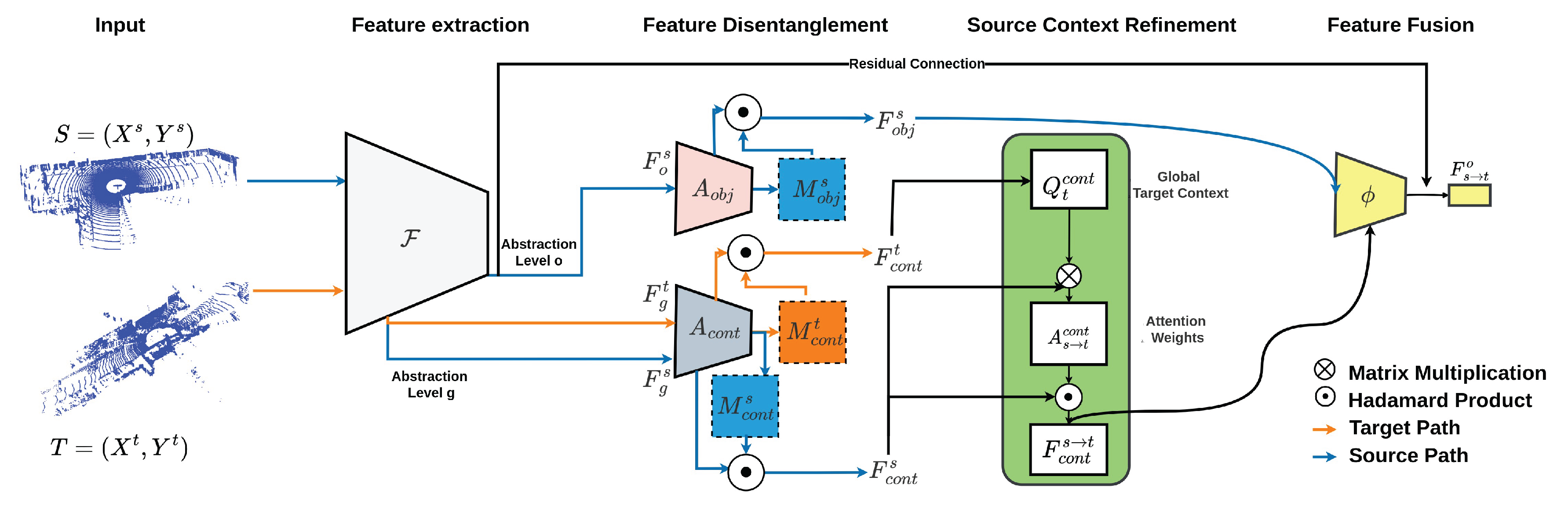
Figure 2.
Illustration of how the features of two points (highlighted in yellow) are calculated using : (a) Squeeze and Excitation attention module. (b) Vector self attention. (c) Our proposed attention mechanism for object and context feature refinement.
Figure 2.
Illustration of how the features of two points (highlighted in yellow) are calculated using : (a) Squeeze and Excitation attention module. (b) Vector self attention. (c) Our proposed attention mechanism for object and context feature refinement.
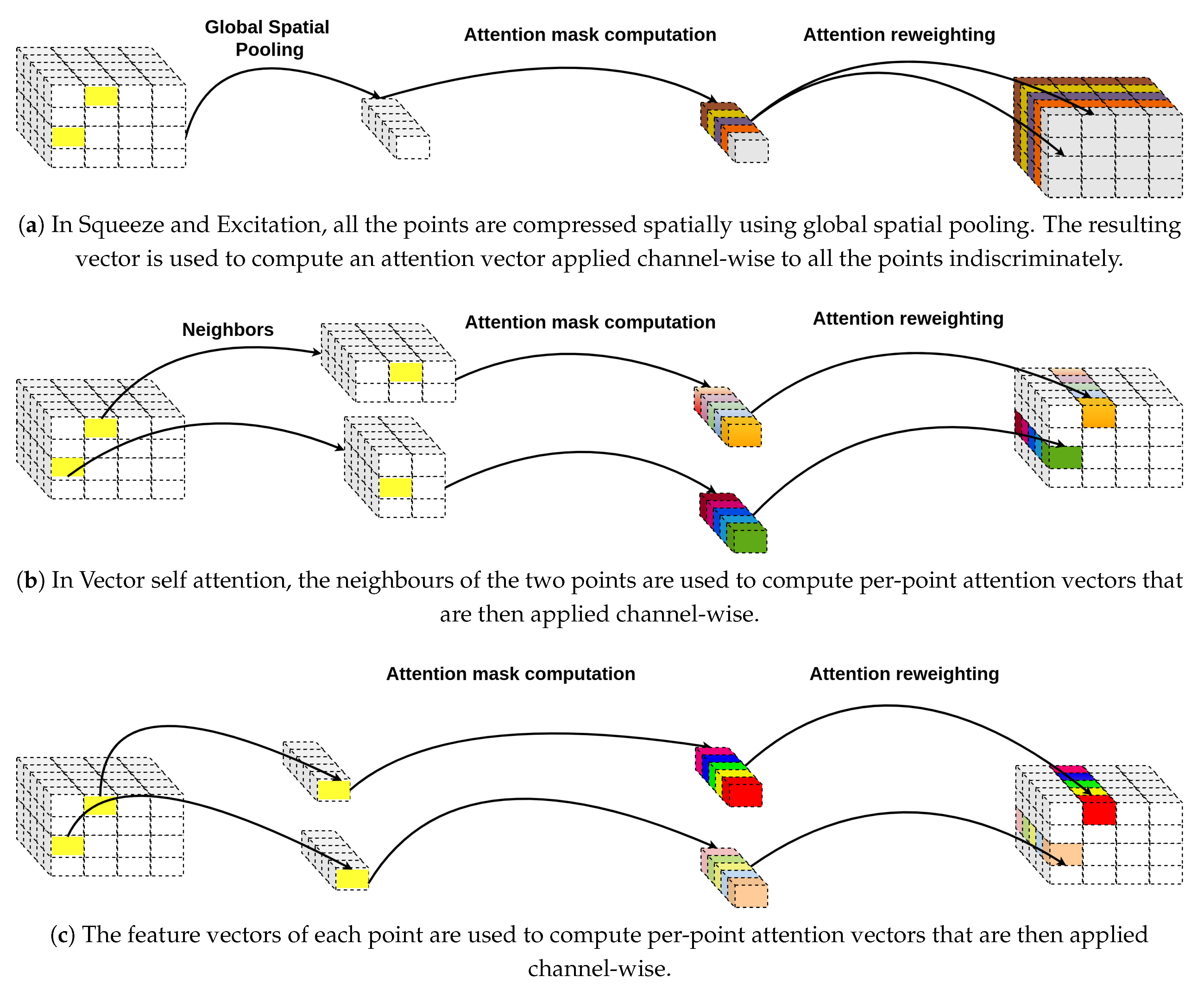
Figure 3.
Object and context attention maps for two example point clouds. (a,b) Input point clouds. (c,d) Object attention maps highlighting object-specific features. Points relevant to objects are highlighted in green. (e,f) Context attention maps emphasizing contextual information. Points important for scene context are highlighted in green.
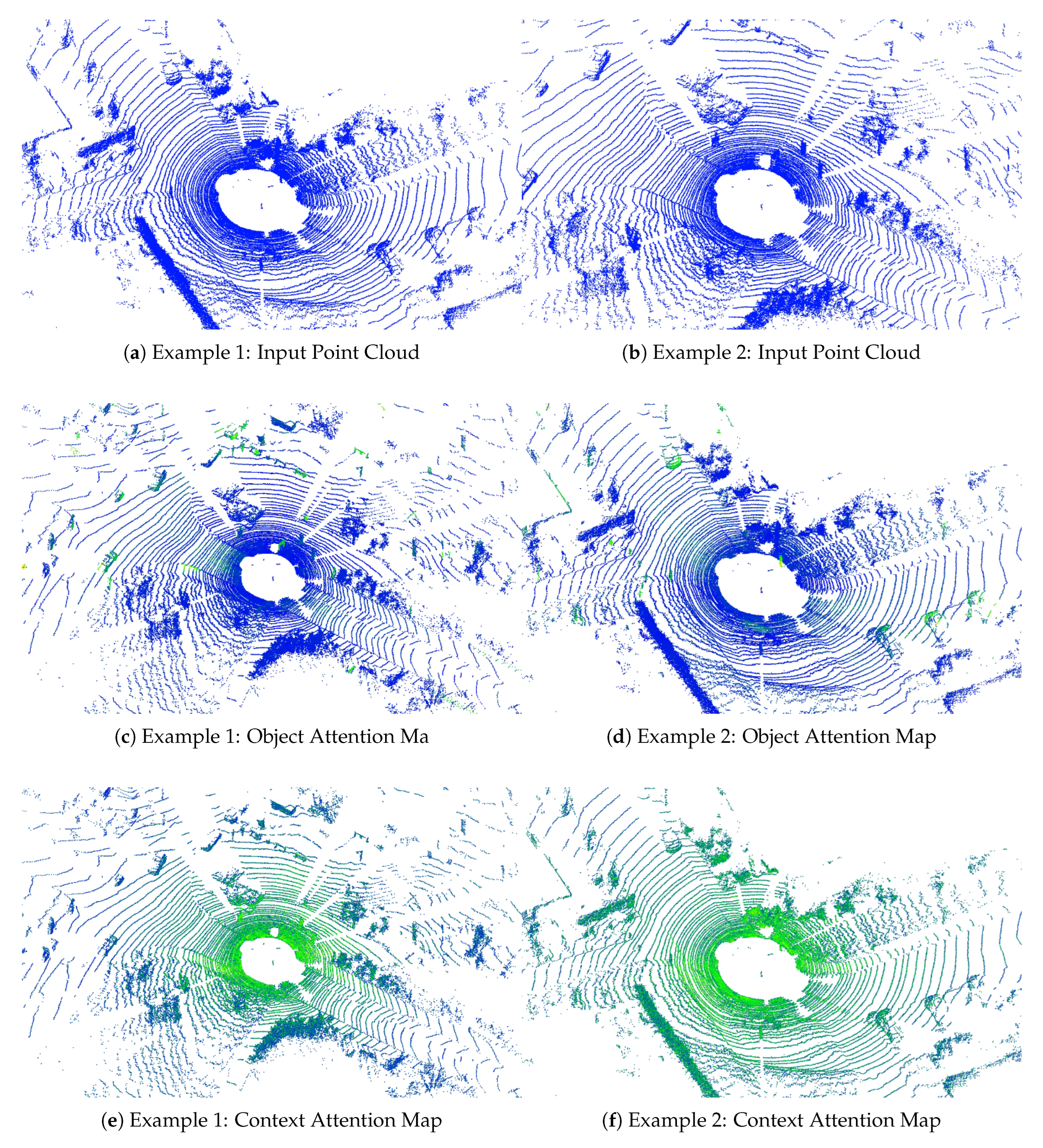
Figure 4.
Segmentation comparison on SynLiDAR → SemanticPOSS. Two example scenes are shown, comparing Ground Truth, CoSMix, and our CAFA method.
Figure 4.
Segmentation comparison on SynLiDAR → SemanticPOSS. Two example scenes are shown, comparing Ground Truth, CoSMix, and our CAFA method.
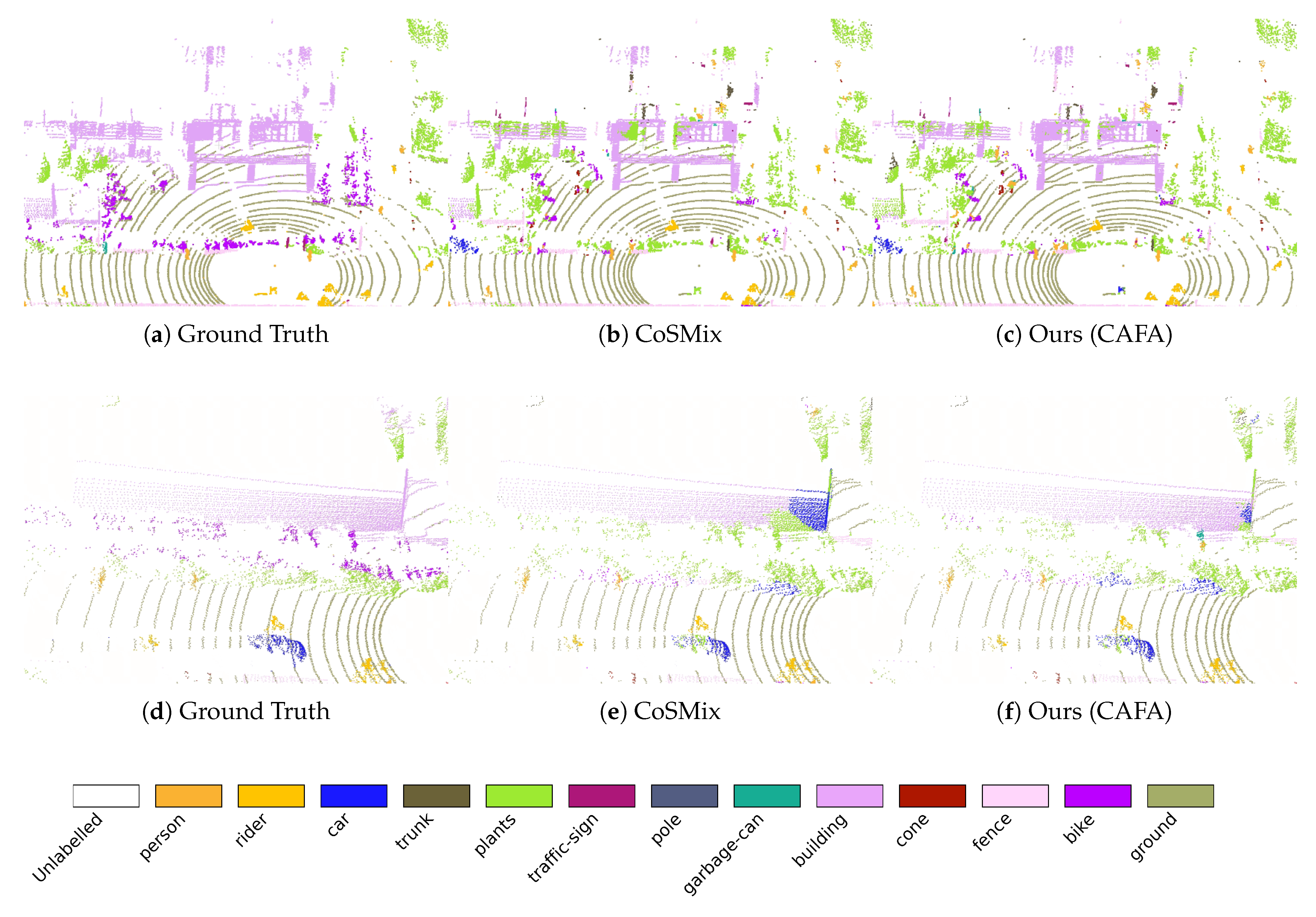
Figure 5.
Segmentation comparison on SynLiDAR → SemanticKITTI. Three example scenes are shown, comparing Ground Truth, CoSMix, and our CAFA method.
Figure 5.
Segmentation comparison on SynLiDAR → SemanticKITTI. Three example scenes are shown, comparing Ground Truth, CoSMix, and our CAFA method.
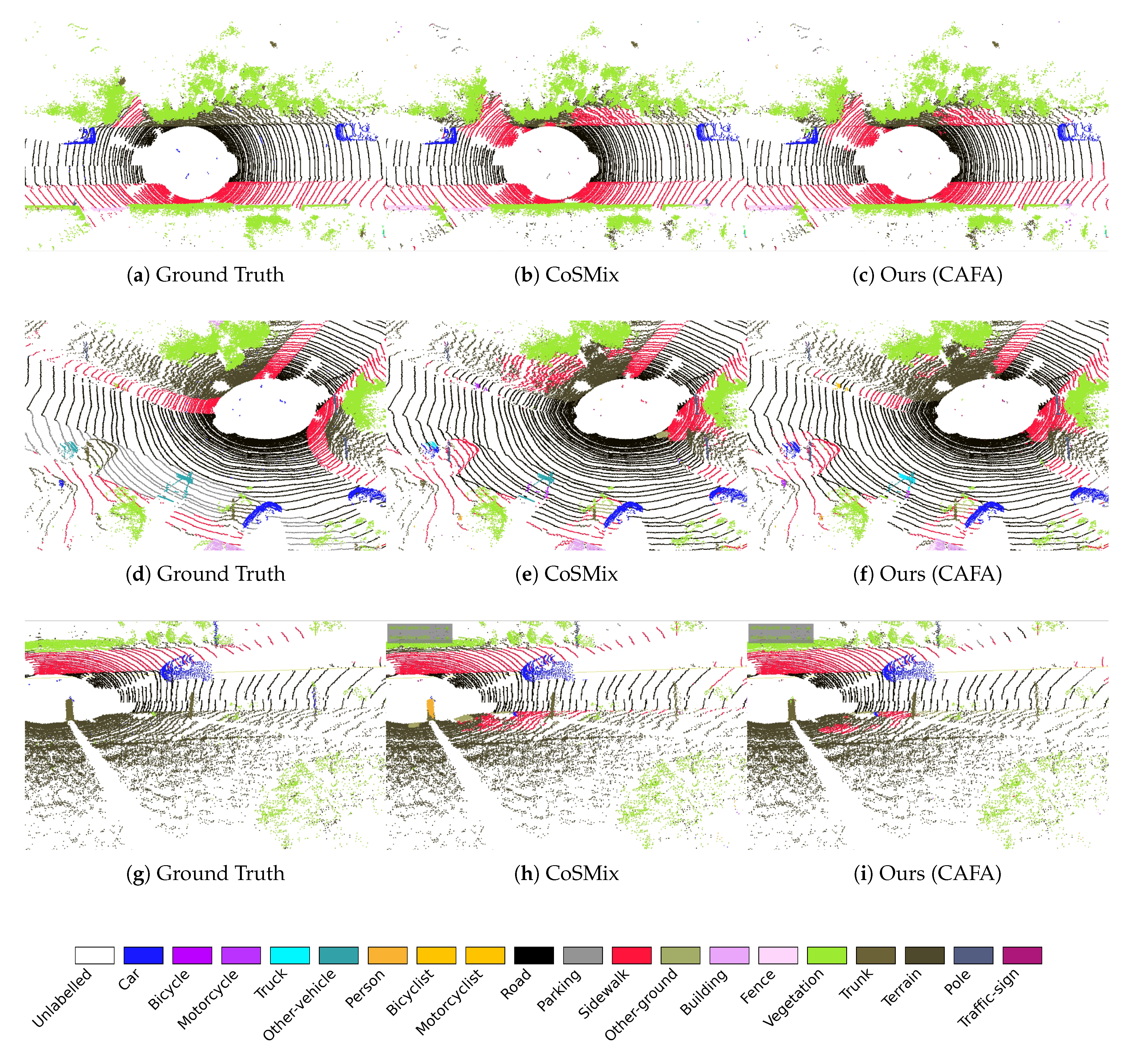
Figure 6.
Analysis of our approach in mitigating negative transfer for sidewalk segmentation.
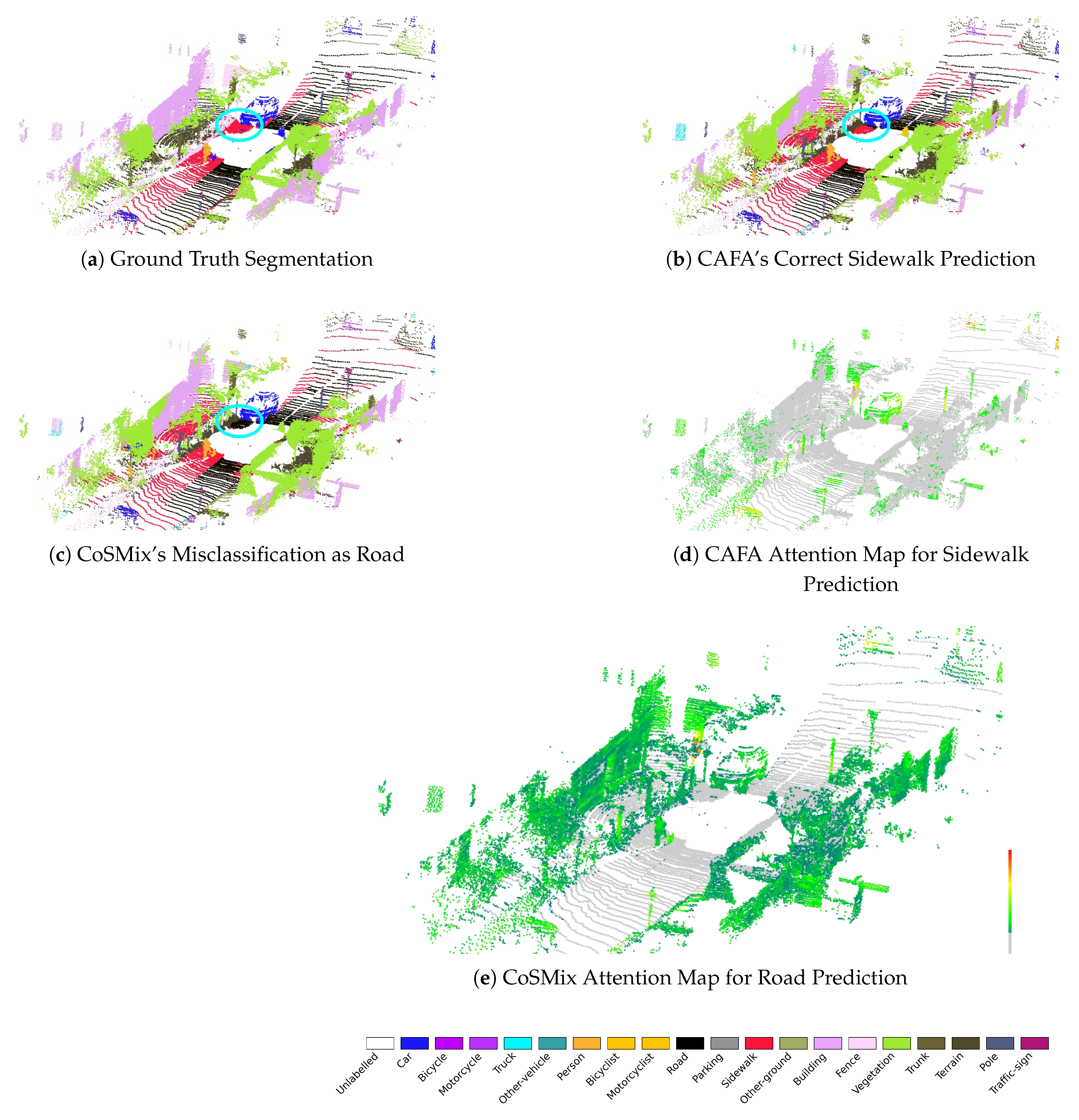
Figure 7.
Co-occurrence matrices for source (SynLiDAR) and target domains. (a) shows the co-occurrence matrix for SynLiDAR. (b) shows the co-occurrence matrix for SemanticPOSS. The observed differences result from the distinct class mappings applied during the domain adaptation process.The color intensity represents the frequency of co-occurrence between classes.
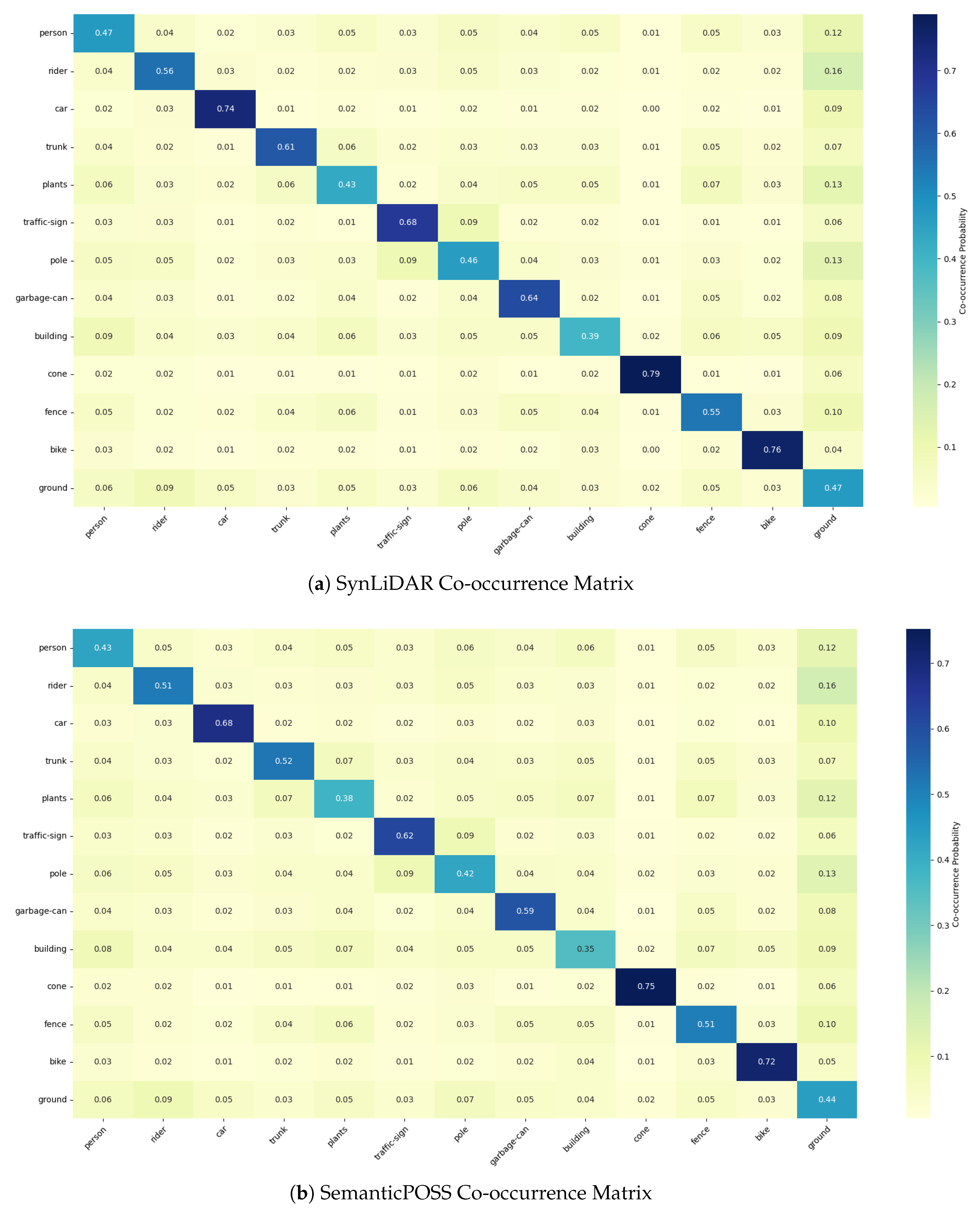
Figure 8.
Co-occurrence matrices for source (SynLiDAR) and target domains. (a) shows the co-occurrence matrix for SynLiDAR. The observed differences result from the distinct class mappings applied during the domain adaptation process. (b) shows the co-occurrence matrix for SemanticKITTI. The color intensity represents the frequency of co-occurrence between classes.
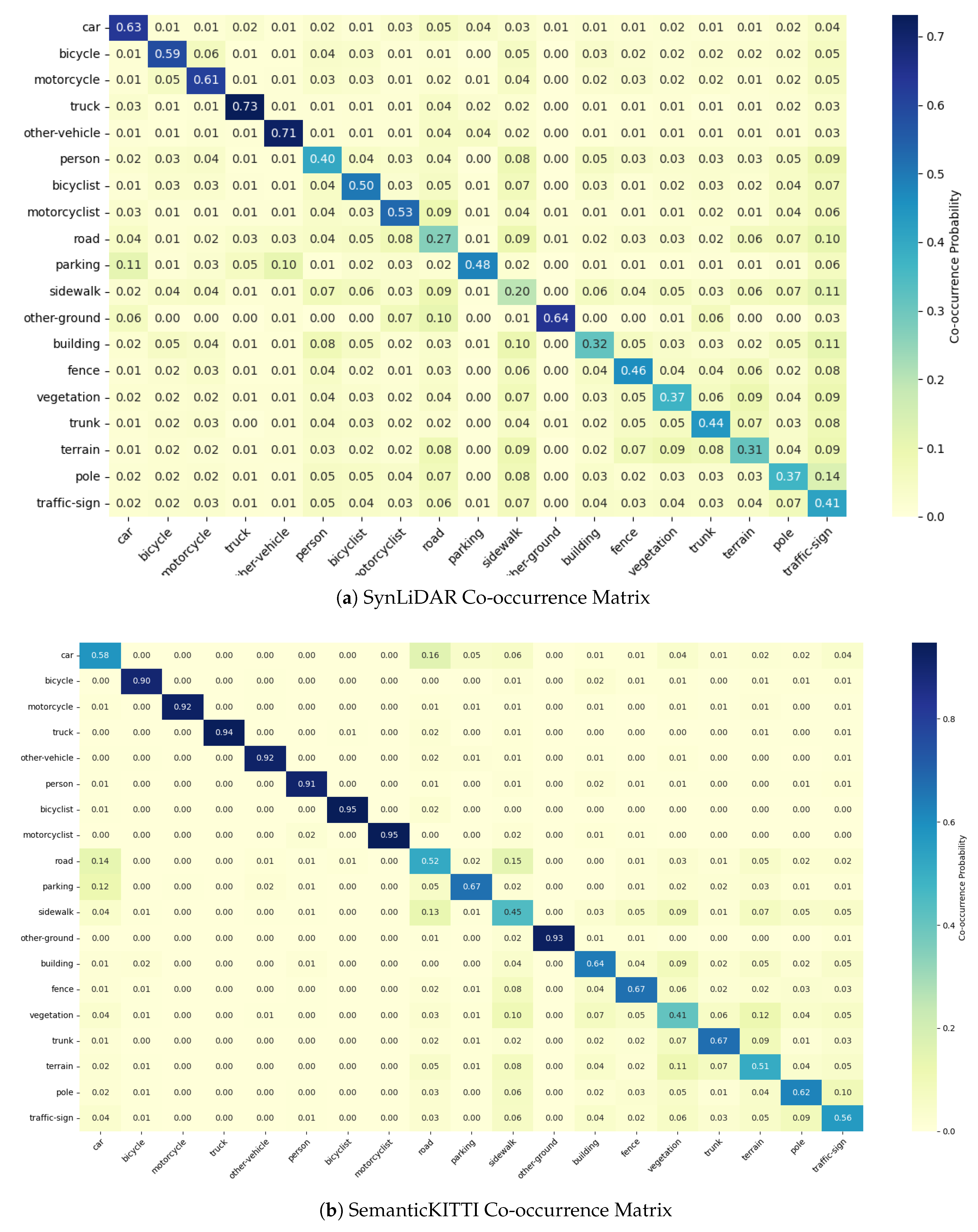
Figure 9.
Class-wise performance gain (IoU difference) against context shift magnitude. X-axis: per class L1 distance between source/target co-occurrence matrices. Y-axis: IoU improvement. Each point represents a class; trend lines show correlation between shift and performance gain.
Figure 9.
Class-wise performance gain (IoU difference) against context shift magnitude. X-axis: per class L1 distance between source/target co-occurrence matrices. Y-axis: IoU improvement. Each point represents a class; trend lines show correlation between shift and performance gain.
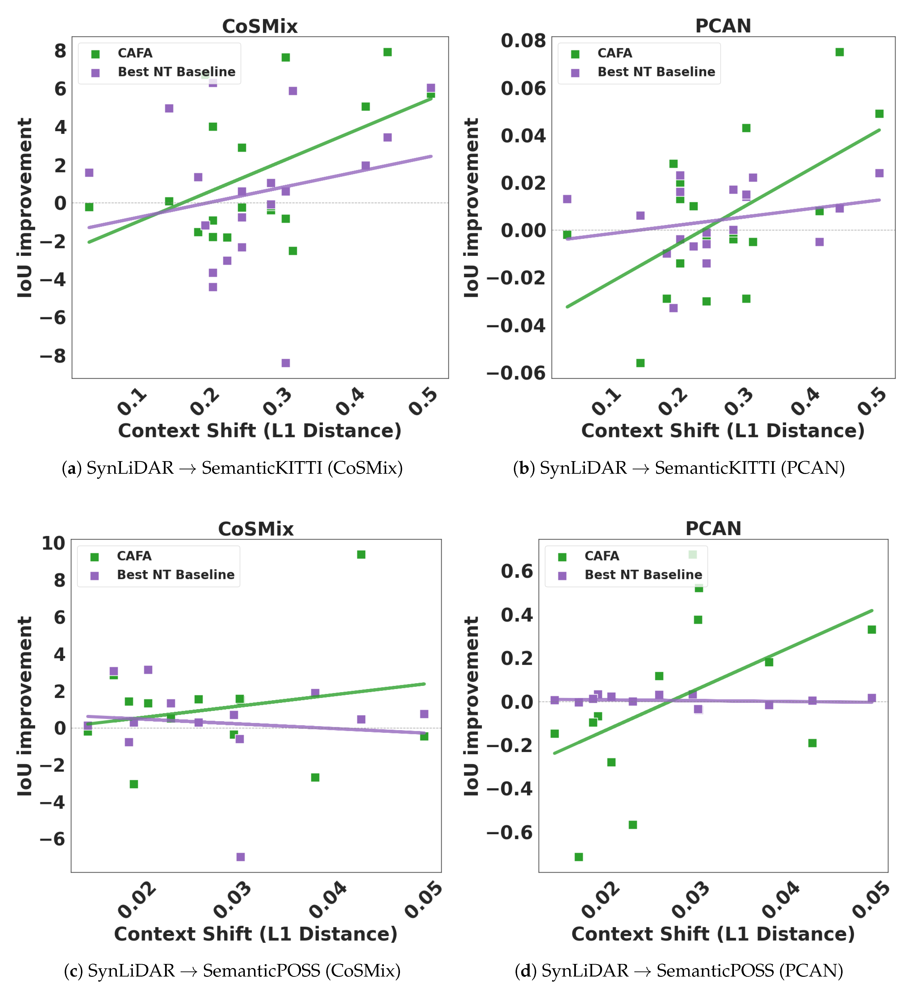

Table 1.
Main hyperparameters for PCAN training.
| Hyperparameter | SemanticKITTI | SemanticPOSS |
|---|---|---|
| Maximum Epochs | 100000 | 100000 |
| Entropy Threshold | 0.05 | 0.05 |
| Adversarial Loss Weight | 0.001 | 0.001 |
| Mean Teacher | 0.9999 | 0.9999 |
| Voxel Size | 0.05 | 0.05 |
| Learning Rate (Generator) | 2.5e-5 | 2.5e-4 |
| Learning Rate (Discriminator) | 1e-5 | 1e-4 |
Table 2.
Main hyperparameters for CoSMix.
| Hyperparameter | SemanticKITTI | SemanticPOSS |
|---|---|---|
| Voxel Size | 0.05 | 0.05 |
| Number of Points | 80000 | 50000 |
| Epochs | 20 | 20 |
| Train Batch Size | 1 | 1 |
| Optimizer | SGD | SGD |
| Learning Rate | 0.001 | 0.001 |
| Selection Percentage | 0.5 | 0.5 |
| Target Confidence Threshold | 0.90 | 0.85 |
| Mean Teacher | 0.9 | 0.99 |
| Teacher update frequency | 500 | 500 |
Table 3.
Adaptation results on SynLiDAR → SemanticKITTI. The source corresponds to the model trained on the source dataset. Results are reported in terms of mean Intersection over Union (mIoU).
Table 3.
Adaptation results on SynLiDAR → SemanticKITTI. The source corresponds to the model trained on the source dataset. Results are reported in terms of mean Intersection over Union (mIoU).
| Model | car | bike | mot | truck | other-v | perso | bcyst | mclst | road | park | sidew | other-g | build | fence | vege | trunk | terra | pole | traff | mIoU | gain |
|---|---|---|---|---|---|---|---|---|---|---|---|---|---|---|---|---|---|---|---|---|---|
| Source | 72.6 | 6.7 | 11.6 | 3.7 | 6.7 | 22.5 | 29.5 | 2.8 | 67.2 | 11.9 | 35.7 | 0.1 | 59.9 | 23.5 | 74.3 | 25.7 | 42.0 | 39.6 | 13.3 | 28.9 | - |
| CoSMix [3] | 83.6 | 10.2 | 14.4 | 8.8 | 15.2 | 27.4 | 23.5 | 0.7 | 77.4 | 17.4 | 43.6 | 0.3 | 55.1 | 24.5 | 72.7 | 44.8 | 40.8 | 45.3 | 19.8 | 32.9 | +0.0 |
| CoSMix + CWFT[29] | 85.1 | 11.2 | 14.3 | 4.0 | 11.9 | 28.0 | 16.5 | 3.9 | 76.4 | 16.9 | 44.9 | 0.1 | 52.1 | 25.2 | 72.4 | 42.2 | 42.8 | 44.2 | 19.6 | 32.2 | -0.7 |
| CoSMix + DSAN[19] | 84.6 | 1.8 | 15.0 | 5.1 | 10.7 | 33.5 | 26.9 | 2.7 | 76.6 | 18.8 | 44.2 | 0.2 | 61.0 | 30.8 | 74.3 | 41.8 | 39.6 | 42.9 | 24.8 | 33.4 | +0.5 |
| CoSMix + TransPar[26] | 83.8 | 5.4 | 13.1 | 7.1 | 13.0 | 22.5 | 15.4 | 2.5 | 77.2 | 17.3 | 43.4 | 0.1 | 58.6 | 24.9 | 73.4 | 41.6 | 38.5 | 43.5 | 15.8 | 31.4 | -1.5 |
| CoSMix + BSS[24] | 82.6 | 5.3 | 17.4 | 7.8 | 11.7 | 26.7 | 12.7 | 3.5 | 77.5 | 19.9 | 44.6 | 0.2 | 52.5 | 25.9 | 72.1 | 38.9 | 41.1 | 43.4 | 20.1 | 31.8 | -1.2 |
| CoSMix + CAFA (ours) | 83.2 | 9.4 | 22.1 | 7.9 | 13.4 | 33.2 | 31.4 | 5.7 | 78.0 | 15.9 | 46.5 | 0.1 | 52.6 | 28.5 | 72.5 | 43.0 | 47.5 | 45.0 | 19.9 | 34.5 | +1.6 |
| PCAN [4] | 85.6 | 16.2 | 27.4 | 9.9 | 10.4 | 28.4 | 64.2 | 2.9 | 77.1 | 13.9 | 50.3 | 0.1 | 67.4 | 19.4 | 75.9 | 41.4 | 47.7 | 40.8 | 21.7 | 36.9 | +0.0 |
| PCAN + CWFT[29] | 86.6 | 17.0 | 25.7 | 10.9 | 10.1 | 30.6 | 60.1 | 2.7 | 77.4 | 12.8 | 50.1 | 0.1 | 64.9 | 23.3 | 74.7 | 43.6 | 46.5 | 42.7 | 22.8 | 37.0 | +0.1 |
| PCAN + DSan[19] | 85.8 | 16.9 | 27.7 | 9.9 | 10.3 | 28.7 | 65.3 | 2.8 | 77.0 | 14.2 | 50.4 | 0.1 | 69.0 | 19.9 | 76.4 | 42.1 | 46.6 | 41.4 | 22.1 | 37.2 | +0.3 |
| PCAN + TransPar[26] | 87.3 | 17.6 | 28.9 | 11.5 | 12.7 | 30.8 | 65.1 | 2.4 | 76.5 | 12.9 | 48.9 | 0.1 | 69.6 | 19.0 | 77.2 | 40.7 | 44.4 | 40.7 | 22.3 | 37.3 | +0.4 |
| PCAN + BSS[24] | 86.0 | 17.0 | 28.1 | 10.5 | 11.6 | 26.9 | 65.9 | 3.3 | 77.2 | 13.9 | 50.3 | 0.1 | 68.1 | 19.4 | 76.2 | 41.2 | 47.4 | 40.7 | 22.9 | 37.2 | +0.3 |
| PCAN + CAFA (ours) | 85.2 | 13.3 | 31.7 | 11.2 | 12.4 | 33.3 | 71.7 | 3.7 | 77.0 | 11.0 | 49.9 | 0.0 | 66.9 | 18.0 | 75.7 | 42.4 | 50.5 | 37.8 | 16.1 | 37.3 | +0.4 |
Table 4.
Adaptation results on SynLiDAR → SemanticPOSS. The source corresponds to the model trained on the source dataset. Results are reported in terms of mean Intersection over Union (mIoU).
Table 4.
Adaptation results on SynLiDAR → SemanticPOSS. The source corresponds to the model trained on the source dataset. Results are reported in terms of mean Intersection over Union (mIoU).
| Model | person | rider | car | trunk | plants | traffic | pole | garbage | building | cone | fence | bike | grou. | mIoU | gain |
|---|---|---|---|---|---|---|---|---|---|---|---|---|---|---|---|
| Source | 45.7 | 40.2 | 51.5 | 22.1 | 71.9 | 4.9 | 22.2 | 21.9 | 71.9 | 4.8 | 29.8 | 2.6 | 76.1 | 35.8 | - |
| CoSMix [3] | 55.3 | 52.4 | 47.6 | 43.5 | 72.0 | 13.7 | 40.9 | 35.4 | 67.7 | 30.2 | 35.3 | 5.6 | 81.3 | 44.0 | +0.0 |
| CoSMix + CWFT[29] | 53.9 | 50.7 | 54.0 | 31.2 | 72.6 | 13.2 | 41.8 | 35.7 | 69.9 | 28.4 | 31.6 | 7.1 | 81.3 | 43.9 | -0.1 |
| CoSMix + DSAN[19] | 52.8 | 51.5 | 51.6 | 35.9 | 70.8 | 13.3 | 38.2 | 36.9 | 62.7 | 31.8 | 33.0 | 4.8 | 79.1 | 43.3 | -0.7 |
| CoSMix + Transpar[26] | 54.6 | 54.1 | 53.2 | 35.4 | 74.1 | 13.7 | 40.7 | 31.5 | 72.8 | 24.4 | 32.9 | 6.3 | 81.1 | 44.2 | +0.2 |
| CoSMix + BSS[24] | 55.6 | 52.7 | 48.0 | 35.2 | 73.3 | 15.5 | 40.1 | 28.4 | 70.8 | 29.6 | 38.4 | 6.2 | 81.4 | 44.3 | +0.3 |
| CoSMix + CAFA (ours) | 52.3 | 53.9 | 56.9 | 34.0 | 72.5 | 11.0 | 42.3 | 36.9 | 70.6 | 31.7 | 36.6 | 5.2 | 81.1 | 45.0 | +1.0 |
| PCAN [4] | 60.9 | 52.3 | 60.1 | 41.2 | 74.5 | 18.0 | 35.0 | 23.9 | 74.8 | 8.0 | 38.7 | 12.3 | 79.3 | 44.6 | +0.0 |
| PCAN + CWFT[29] | 59.7 | 51.5 | 59.1 | 40.9 | 74.0 | 17.6 | 35.0 | 24.8 | 74.4 | 8.7 | 40.2 | 11.3 | 79.2 | 44.3 | -0.3 |
| PCAN + DSAN[19] | 62.3 | 50.3 | 60.7 | 41.3 | 74.9 | 13.3 | 36.9 | 21.4 | 75.4 | 1.9 | 42.7 | 9.9 | 77.6 | 43.7 | -0.9 |
| PCAN + TransPar[26] | 64.0 | 55.2 | 60.4 | 42.8 | 74.5 | 16.3 | 36.1 | 19.9 | 74.3 | 4.5 | 40.9 | 15.4 | 79.9 | 44.9 | +0.3 |
| PCAN + BSS[24] | 62.2 | 52.5 | 60.5 | 38.7 | 74.6 | 20.0 | 35.6 | 18.3 | 77.1 | 4.2 | 44.4 | 14.1 | 79.8 | 44.8 | +0.2 |
| PCAN + CAFA (ours) | 64.4 | 54.0 | 63.9 | 40.9 | 74.1 | 17.7 | 36.0 | 25.2 | 76.0 | 3.2 | 45.5 | 10.7 | 79.7 | 45.5 | +0.9 |
Table 5.
Ablation study results on SynLiDAR → SemanticPOSS.
| Method | mIoU | mIoU |
|---|---|---|
| CAFA (Full) | 45.0 | 0.0 |
| CAFA w/o fusion (simple summation) | 44.3 | -0.7 |
| CAFA w/ single-scale features | 44.1 | -0.9 |
| CAFA w/ object features only | 44.6 | -0.4 |
| CAFA w/o residual connection | 42.4 | -2.8 |
| CAFA w/ self-attention (source) | 44.2 | -0.8 |
| CAFA w/ self-attention (target) | 43.7 | -1.3 |
| CAFA w/ 3D context module [37] | 43.2 | -1.8 |
Table 6.
mIoU (%) for top 3 classes with greatest context shift for SynLiDAR→ SemanticKITTI and SynLiDAR → SemanticPOSS
Table 6.
mIoU (%) for top 3 classes with greatest context shift for SynLiDAR→ SemanticKITTI and SynLiDAR → SemanticPOSS
| Dataset | Class | PCAN | CoSMix | ||||
|---|---|---|---|---|---|---|---|
| Baseline | +NT | +CAFA | Baseline | +NT | +CAFA | ||
| SynLiDAR → SemanticKITTI |
person | 28.4 | 30.8 | 33.3 | 27.4 | 33.47 | 33.18 |
| bicyclist | 64.2 | 65.1 | 71.7 | 23.4 | 26.89 | 31.36 | |
| motorcyclist | 2.9 | 2.4 | 3.7 | 0.7 | 2.66 | 5.74 | |
| mIoU | 31.8 | 32.7 | 36.2 | 17.2 | 21.0 | 23.4 | |
| SynLiDAR → SemanticPOSS |
Trunk | 41.2 | 42.8 | 74.1 | 34.48 | 35.22 | 34.03 |
| Car | 60.1 | 60.4 | 40.9 | 47.57 | 48.02 | 56.94 | |
| Traffic-sign | 18.0 | 16.3 | 36.0 | 13.65 | 15.54 | 10.96 | |
| mIoU | 39.7 | 39.8 | 50.3 | 31.9 | 32.9 | 33.9 | |
Disclaimer/Publisher’s Note: The statements, opinions and data contained in all publications are solely those of the individual author(s) and contributor(s) and not of MDPI and/or the editor(s). MDPI and/or the editor(s) disclaim responsibility for any injury to people or property resulting from any ideas, methods, instructions or products referred to in the content. |
© 2025 by the authors. Licensee MDPI, Basel, Switzerland. This article is an open access article distributed under the terms and conditions of the Creative Commons Attribution (CC BY) license (http://creativecommons.org/licenses/by/4.0/).
Copyright: This open access article is published under a Creative Commons CC BY 4.0 license, which permit the free download, distribution, and reuse, provided that the author and preprint are cited in any reuse.


