Submitted:
25 June 2025
Posted:
26 June 2025
You are already at the latest version
Abstract
Microgravity investigations are widely applied today to address various environmental and geological problems. Unfortunately, this geophysical survey type is comparatively rarely used to search for the hidden ancient targets. It is primarily caused by the small geometric size of the desired archaeological objects and various types of noise that complicate the analysis of the proper signal. At the same time, the development of a modern generation of gravimetric field equipment enables the registration of digital microGal (10-8 m/s2) anomalies, presenting a new challenge in this direction. Correspondingly, the accuracy of gravity variometers (gradientometers) is also sharply increased. A review of microgravity searching and localization of archeological remains of different sizes and types is given. It is shown that the development of Physical-Archaeological Models (PAMs) increases the effectiveness of the geophysical process. A quantitative interpretation methodology for gravity anomalies in complex physical-geological conditions, based on non-conventional solutions transferred from magnetic prospecting, is briefly explained. Advanced 3D modeling of a gravity field elucidated the peculiarities of ancient target delineation under complex physical and environmental conditions. Calculating the second and third derivatives of the gravity potential helps reveal some peculiarities of the different PAMs. Many types of archaeological targets in the world have been categorized by their density and geometrical characteristics into several groups. The model computations and archaeological-geophysical reviews indicate that microgravity investigations may be successfully applied to at least 20% of the available archaeological sites worldwide. The numerous examples supplement the review presented. The further development of the microgravity studies is also discussed.
Keywords:
microgravity
; physical-archaeological models
; quantitative interpretation
; 3D modeling
; gravity field derivatives
; archaeological remains
1. Introduction
Development of a new modern gravimetric and variometric (gradientometric) equipment (permitting registering earlier inaccessible minor anomalies and improving the observation methodology) and creation of new methods for gravity data processing and interpretation have triggered the application of microgravity methodology in environmental and economic minerals geophysics.
Microgravity is recognized now as an effective tool for analysis of various geological inhomogeneties in subsurface, including archaeological purposes (Linnington, 1966; Arzi, 1975; Fajklewicz, 1976; Blížkovský, 1979; Lakshmanan and Montlucon, 1987; Slepak, 1999; Di Filippo et al., 2005; Yuan et al., 2006; Abad et al., 2007; Eppelbaum, 2009; Eppelbaum et al., 2010; Panisova et al., 2013; Fais et al., 2015; Gołebiowski et al., 2018; Tianyao et al., 2000; Pašteka et al., 2020, 2022; Eppelbaum, 2022), karst localization (e.g., Colley, 1963; Beres et al., 2001; Rybakov et al., 2001; Debeglia et al., 2006; Eppelbaum, 2007; Eppelbaum et al., 2008; Whitelaw et al., 2008; Al-Zoubi et al., 2013; Ezersky et al., 2023), engineering problems (e.g., Yule et al., 1998; Butler, 2001; Branston and Styles, 2006; Bradley et al., 2007; Khosravi et al., 2019; Porzucek and Loj, 2021), mining and hydrocarbon geophysics (e.g., Sjostrom and Butler, 1996; Karshenbaum et al. 1997; Eppelbaum and Khesin, 2004; Styles et al., 2006; Nind and Seigel, 2007; Slonka, 2011; Gadirov and Eppelbaum, 2012), and volcanology (e.g., Watanabe et al., 1998; Deroussi et al., 2009; Yagi et al., 2024).
Bichara et al. (1981) first identified the specific problems encountered in microgravity investigations. Butler (1984a, 1984b) conducted a thorough investigation of the concepts and corresponding interpretative procedures for gravity and gravity-gradient determination in microgravity. The types of noise (disturbances) arising in the microgravity investigations are studied in detail in Debeglia and Dupont (2002). Styles et al. (2006) discussed several actual problems suggested for removing noise components arising in microgravity under complex environments. The advanced procedures developed, for example, in mining or engineering in microgravity, can be effectively transferred to archaeological investigations and vice versa.
The planning of microgravity investigations must be accompanied by the development of preliminary physical-archaeological models (PAM) (Eppelbaum, 2010). Such PAMs enable the estimation of the expected gravity effects from archaeological targets, allowing for the determination of the area under study, the observation step, GPS observation accuracy requirements, and the necessary accuracy of observations. Then, at subsequent stages, more complex PAMs can be developed that reflect the generalized properties of the archaeological objects being studied.
2. Different Kinds of Noise Appearing in Microgravity Investigations at Archaeological Sites
2.1. Typical kinds of Noise in Microgravity
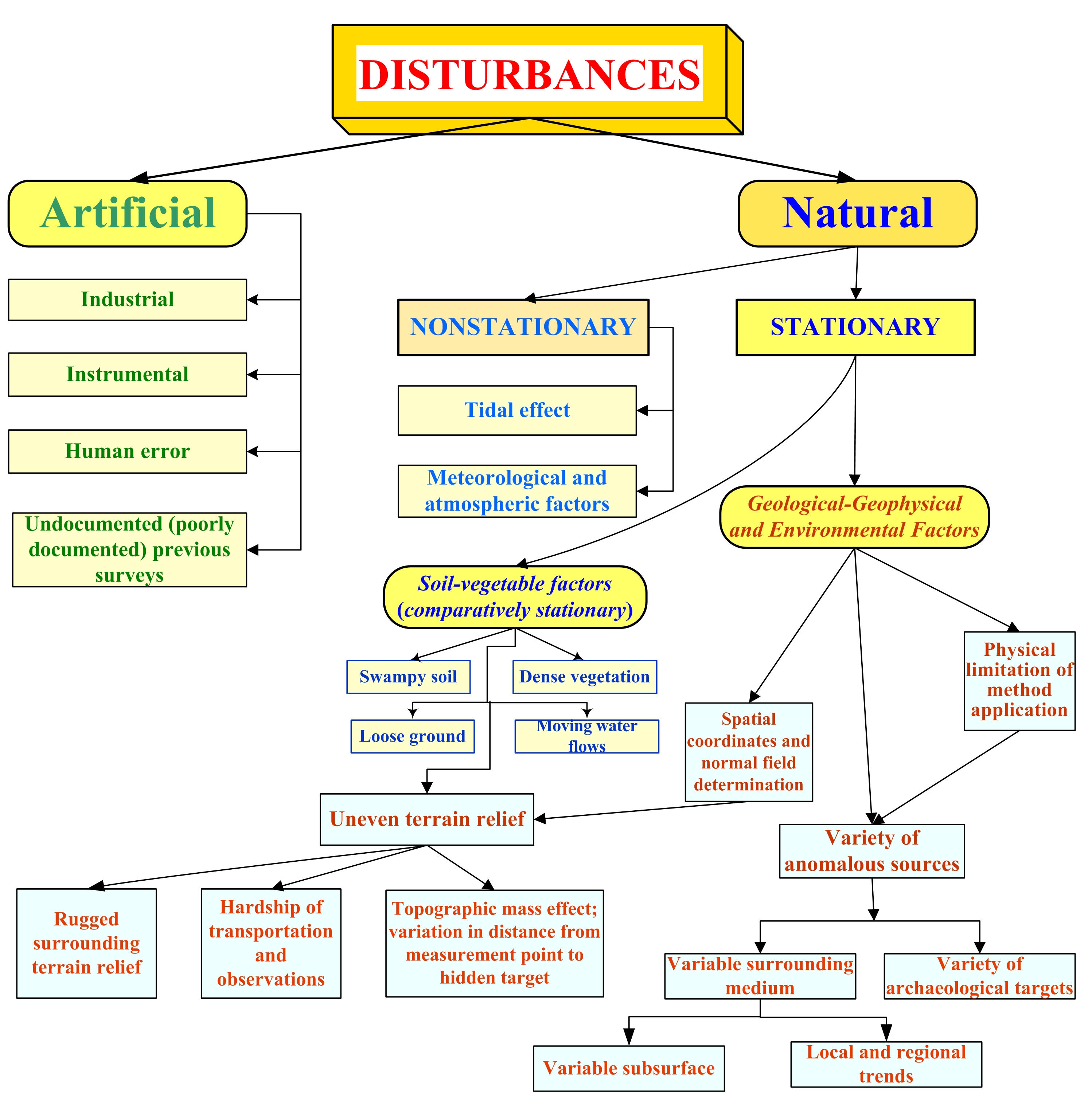
Microgravity surveys in archaeological sites are complicated by several kinds of noise (Eppelbaum et al. 2010, 2011) (Figure 1). These disturbances are briefly considered below.
Artificial (Man-Made) Disturbances
The industrial component of noise mainly arises from surrounding buildings, engineering constructions, and various underground and transportation systems. The instrumental component is associated with the ‘shift zero’ and other technical properties of gravimeters (variometers) and their spatial locations. Human errors, notably, can accompany geophysical observations at any time. Finally, poorly documented (or undocumented) results from previous surveys can distort the preliminary development of the PAM.
Natural Disturbances
The Natural noise (disturbances) can be subdivided into Nonstationary and Stationary. Nonstationary noise includes the tidal variations, mainly from the Moon and the Sun’s attraction, and some variations associated with the geodynamic events at depth. Meteorological and atmospheric factors reflect changing pressure, temperature, humidity, and electrical fields. Such meteorological conditions as rain, lightning, snow, and hurricanes hamper the microgravity observations, too. Soil-vegetation factors associated with specific soil types (e.g., swampy soil or loose ground in deserts) and dense vegetation, which can sometimes hinder movement along the profile, also need to be considered. Finally, the movement of water in basins and rivers can also affect the readings.
Stationary disturbances consist of two main components. First are Geological-geophysical and archaeological factors. The application of any geophysical method depends primarily upon the existence of physical property differences between the objects under study and the surrounding medium. The physical limitations of the methods reflect measurable density contrast properties between the archaeological targets and the geo-environmental sequence. The thermal-density dependence of sedimentary rocks, as discovered by Gadirov and Eppelbaum (2015), may necessitate reinterpreting the results of some detailed gravity surveys in archaeological sites (where sedimentary thickness exceeds 4-5 meters). The spatial coordinate determination plays a significant role in microgravity, as even a slight inaccuracy in the coordinates yields a value compatible with the expected anomalies from the archaeological targets.
The variety of anomalous sources is composed of two factors: the variable surrounding medium and the variety of archaeological targets; both aspects are crucial and greatly complicate the interpretation of microgravity data. Additional disturbances can introduce the variable subsurface and various gravity trends.
The separate group of disturbances creates obvious Soil-vegetation factors, as land microgravity measurements cannot be carried out in unfavorable environmental conditions.
Uneven terrain relief has three branches: (1) Rugged surrounding terrain relief (which can be removed or eliminated by Terrain Correction), (2) Hardship of observations (the author of this paper has performed the gravity observations at the Greater Caucasus on the inclined relief with an angle of almost 40o), and (3) Topographic mass effect which is generally twofold and involves the form and physical properties of the topographic features of the terrain relief as well as the effect of variations in the distance from the point of measurement to the hidden target (Eppelbaum, 2022).
The possibility of reducing topographic effects by grouping points of additional gravimetric observations around the central point located on the survey network was demonstrated in Khesin et al. (1996). A group of 4 to 8 extra points is situated above and below along the relief, approximately symmetrically and equidistant from the central point. The topographic effect is reduced to the obtained difference between the gravity field in the center of the group and its mean value for the whole group.
Let us consider the topographic effect, which is very important in microgravity studies, in detail. The correct removal (elimination) of regional gravity trends is not a trivial task (e.g., Telford et al., 1993; Jacoby and Peter, 2009). Figure 2 shows two cases of non-horizontal gravity observations with the presence of an anomalous body occurring close to the Earth’s surface.
The distorting effect of a non-horizontal observation line occurs when the anomalous target differs from the surrounding medium by density, which produces an anomalous vertical gradient. Analysis of the ΔgB anomalies observed on the horizontal and inclined rugged relief indicates that the gravity effects in these situations are cardinal different (Figure 2).
Although the Bouguer reductions were applied to the observations on the inclined relief, the computed Bouguer anomaly is characterized by the small negative values in the downward direction of the relief, whereas the anomaly on the horizontal profile has no negative values. Theoretically, it is not possible since the gravity effect from a body with a positive contrast density (750 kg/m3) occurring in the homogenous medium must be only positive and tend to zero at far distances from the target.
Thus, applying the conventional corrections does not eliminate this trend because the observation points for the anomalous object are significantly different, and the large anomalous body occurs close to the observation points (Eppelbaum, 2011). Hence, a special methodology is required for the gravimetric quantitative interpretation of anomalies observed in the rugged relief conditions (see next section).
2.2. Terrain Correction Applied for High-Accuracy Gravity Investigations: Two Nonconventional Approaches
How can we enhance the effectiveness and reliability of interpretation? Undoubtedly, it must be a multi-stage process. We must begin with nonconventional methodologies for reducing the surrounding topographic effect and terrain correction computation.
It is well known that the accuracy of microgravity investigations substantially depends on the accuracy of terrain correction (TC) computing. The two approaches presented below were applied to calculate the exact TC for the detailed Bouguer gravity observations at ore deposits in the Lesser and Greater Caucasus.
2.2.1. First Approach
The first method was applied in the Gyzylbulakh gold-pyrite deposit, situated in the Mekhmana ore region of Azerbaijan (Garabagh, Lesser Caucasus), under conditions of rugged relief. This deposit has been thoroughly investigated through mining and drilling operations; therefore, it was used as a reference field polygon for testing this approach. A special scheme for obtaining the Bouguer anomalies has been employed to suppress the terrain relief effects, thereby dampening the anomaly effects from the objects being prospected. The scheme is based on calculating the difference between the free-air anomaly and the gravity field determined from a 3D model of a uniform medium with a real topography. A 3-D terrain relief model with an interval of 80 km (six investigated profiles of 800 m length are in the center of this interval) was employed to compute (using GSFC software) the gravitational effect of the medium (σ = 2670 kg/m3). By applying such a scheme, the Bouguer anomalies were obtained with an accuracy two times higher than that of TC received by the conventional methods. As a result, based on the improved Bouguer gravity with the precise TC data, the geological structure of the deposit was defined (Eppelbaum, 2019).
2.2.2. Second Approach
The second approach was employed at the complex Katekh pyrite-polymetallic deposit, which is located at the southern slope of the Greater Caucasus (northern Azerbaijan). The main peculiarities of this area are the very rugged topography of a SW-NE trend, complex geology, and severe tectonics. Despite the availability of conventional ΔgB (TC of far zones were computed up to 200 km), a digital terrain relief model was created to enhance the calculation of surrounding terrain topography (Eppelbaum and Khesin, 2004). The SW-NE regional topography trend in the Katekh deposit occurrence was computed as a rectangular digital terrain relief model (DTRM) of 20 km long and 600 m wide (our interpretation profile with a length of 800 m was in the geometrical center of the DTRM). About 1,000 characteristic points were used to describe the DTRM (most frequently, these points were focused on the center of the DTRM, and more rarely, on the margins). Thus, in the interactive 3D ΔgB modeling (using GSFC software), the effect was computed not only from geological bodies occurring in this area but also from the surrounding DTRM. In the issue of this scheme application, two new ore bodies were discovered (Eppelbaum and Khesin, 2004).
3. Feasibility of Microgravity Application at Different Types of Archaeological Sites in the World
Let us consider the application of the microgravity technique to various types of archaeological targets worldwide.
3.1. Egyptian Pyramids
Egyptian pyramids are significant (and not fully understood to this day) archaeological objects where microgravity studies can introduce crucial information. Kerisel (1988) employed the microgravity method to estimate the weight and peculiarities of the Cheops pyramid (Egypt). Lakshmanan and Montlucon (1987), Lakshmanan (1991), and Issawy and Radwan (2012) conducted microgravity investigations inside, above, and around the Cheops pyramid, leading to an evaluation of the structure’s overall density and density changes within the structure. Saleh et al. (2022) have detected two buried chambers and an unrecognized negative gravity trench at the Pyramid of Senusret II, Lahun, Fayoum, Egypt.
The potential possibilities of microgravity investigations have not been fully explored. An integrated analysis of Δg, Δgx, and Δgz carried out at different levels will enable a more precise interpretation of the complex gravity patterns from these enigmatic objects. A comprehensive estimation of the expected gravity effects was demonstrated in Pašteka et al. (2022).
Ivashov et al. (2023) proposed generalizations of previous investigations and a perspective on using a UAV to deliver a gravimeter to the desired point on the step surface of the Khufu Pyramid.
3.2. Ancient Underground Caves
A careful examination of microgravity anomaly at the Boden Vean (Cornwall, UK) allowed for the suggestion of new archaeological remains occurring (Linford, 1998). Castiello et al. (2010) have delineated an ancient underground cavity in the complex urban environment of Naples (Italy). The residual gravity map, with the vertical gravity map highlighted, showed the presence of empty cavities or cavities filled with low-density sedimentation in an archaeological site in Sardinia (Italy) (Fais et al., 2015).Chromčák et al. (2018) demonstrated the detection of ancient cavities in the Saint Mary Church (Kláštor, Slovakia), with the obtained results subsequently confirmed by GPR data analysis. Nicolas et al. (2024) study enabled the reliable detection of the ancient pits and voids at the Ouels Mine (Castel-Minier, France).
3.3. Ancient Pavements and Roads
Styles et al. (2006) studied the major collapse that occurred within the ancient Roman road connecting Dover to London. Here, the corrections for the effects of the main open-cut workings and for the influence of surrounding buildings and topography were fruitfully introduced.
A simplified model example of buried pavement delineation is presented in Figure 3. A buried pavement having the positive density contrast of 400 kg/m3 and occurring at a depth of 1.8 m in a uniform medium (PAM of one of the Megiddo sites (Finkelstein and Martin, 2022) was selected as a basis) could be easily recognized by a microgravity survey (Figure 3A, anomalous effect from two bodies). Let us assume a low-density layer (2100 kg/m3) over the pavement. It makes the delineation of the pavement practically impossible in the field conditions (registered anomaly is oscillating about one microGal) (Figure 3A, anomalous effect from three bodies). At the same time, the values of the second vertical derivative of gravity potential Wzz (computed for the levels of 0.3 and 1.5 m) with a measurable accuracy testify to the presence of a disturbing body by anomalies appearing over the pavement’s edges (Figure 3B).
3.4. Ancient Water Reservoirs
Abad et al. (2007) carried out an assessment of a buried rainwater cistern in the Carthusian Monastery (Valencia, Spain) based on 2D microgravity modeling. Ebrahimi et al. (2019) conducted a successful gravity investigation in conjunction with an electric resistivity analysis over the ancient aqueduct (qanat) in northeastern Iran; the qanat was identified by microgravity anomalies of –(10-20) µGal. Bárta et al. (2020) successfully applied detailed gravity surveys to detect old water reservoirs in the historical center of Prague.
A PAM of the buried Roman aqueduct in Israel has been developed on the example of the excavated Caesarea aqueduct (Porath and ‘Ad, 2015). The following parameters were assumed: depth of the HCC center – 2.5-2.8m (σ = 0), radius – 1.2 m, thickness of the aqueduct’s walls – 0.08 m (σ = 2600 kg/m3), the density of the surrounding medium σ = 2100 kg/m3, and length – 200 m. Despite the disturbing effects of the aqueduct walls, the calculated gravity effects were estimated as 10-15 µGal, i.e., quite detectable by the modern gravimeters.
3.5. Ancient Underground Galleries and Tunnels
Fajklewicz’s (1976) investigation was suggested for the examination of the vertical gravity gradient (Wzz) over the underground galleries. He was first indicating the significant difference between the physically measured Wzz and this value obtained via any transformation. Microgravity surveys have been successfully employed at the Roman Amphitheatre of Durres, Albania, both over galleries and walls (Di Filippo et al., 2005). A detailed gravity examination was effectively performed in the Red Square (Moscow) several years ago to delineate the ancient underground galleries (personal communications).
The microgravity survey successfully produced a map of the 150-year Williamson tunnels beneath inner-city Liverpool (England), nicely demonstrating the validity of applying the method to industrial archaeology even in ‘brownfield’ sites (Cuss and Styles, 1999). The precise gravity observations at the National Library court in Moscow enabled the revelation of an earlier unknown tunnel at a depth of 1.5 m (Chernov, 2009). Orfanos and Apostolopoulos (2011) concluded, based on their detection of an ancient tunnel in the Lavrion area (Greece), that a combination of microgravity and resistivity is a powerful interpretive tool. Madej et al. (2018) applied microgravimetry for the delineation of the buried tunnels in Walbrzych, Poland, for searching the ‘Gold Train’ of the Second World War.
3.6. Ancient Building Architecture
Slepak (1999) obtained gravity anomalies of 30-80 microGals reflecting the remains of ancient buildings in the territory of Kazan Kremlin (Russia). Pašteka and Zahorec (2000) examined a complex microgravity anomaly in a former church of St. Catherine (Dechtice, Slovakia) using stripping technology. Yuan et al. (2006) have conducted a comprehensive gravity field modeling over the Emperor Qin Shi Huang Mausoleum (China), where data from other geophysical fields were used to agree on the geometric and density properties. Microgravity anomalies of 15-20 microGals were registered over the remains of the Late Byzantine church walls in Umm er-Rasad (Jordan) (Bataynen et al., 2007). Rabbel et al. (2018) applied a set of geophysical methods to study the Roman church in the city of Iznik (southern Turkey); microgravity studies enabled the localization of a low-density zone in the near-surface, which was interpreted as a grave filled with loose sediment.
Palgiara and di Filippo’s (2009) microgravity survey has led to the detection of remains of walls, foundations, fillings, crypts, and passages in the Basilica of San Paolo fuori le Mura (Rome). The microgravity measurements in the Church of St. George, Svätý Jur (Slovakia) significantly supplemented GPR constructions (Panisova et al., 2016). Detailed gravity-magnetic surveys at Tepe Hissar-Damghan archaeological site, northeastern Iran (Sarlak and Aghajani, 2017) enabled the recognition of earlier unknown chambers and walls. Gołebiowski et al. (2018) have effectively utilized the microgravity technique in conjunction with other geophysical methods to delineate the medieval underground salt chambers in the village of Wiślica, Poland.
Blížkovský (1979) has identified, using the stripping technology, the crypt under the floor of the St. Venceslas Church in the town of Továčov (Czech Republic). Tianyao et al. (2000) outlined the underground palace in the Mao Ling mausoleum (Ming Dynasty) in Shaanxi (China) using a combined analysis of microgravity and vertical gravity gradient data. The microgravimetric prospection inside the Don Church (Valencia, Spain) enabled the localization of the crypt, which was found in the entrance of the church (Padín et al., 2012).
Detailed investigations in the historic centre of Kazan enabled the recognition of remains of ancient walls (Slepak and Nugmanova, 2004). Combined geophysical investigations with application of microgravity in the Late Byzantine ‘Lion Church’ in Umm er-Rasas (Jordan) enabled the identification of floors of a building with the remains of walls, rooms, paths, and foundations(Bataynen et al., 2007). Non-conventional integration of gravity and its horizontal gradient with the radon gas anomalies was performed in the Alkhantepe archaeological monument (Southern Azerbaijan) (Safarov et al., 2019). Calculation of the second derivative of the gravity potential enabled the contour of ancient walls in the Cot Sidi Abdallah site (Morocco) (Sari et al., 2020).
It is well known that in urban or industrial development conditions, methods for calculating gravitational effects from nearby buildings are of great importance. New techniques for solving this problem are described in Pánisová et al. (2012), Yu (2014), Zahorec et al. (2014), and Loj and Porzucek (2019).
3.7. Ancient Cemeteries and Tombs
The Linnington’s (1966) attempt to examine the Etruscan chambered tombs at Cerveteri (Italy) was not very successful but following microgravity applications in archaeology have shown the potential of this method. Detailed gravity survey in the Kenchreai cemetery (southern Greece) enabled the reliable localization of two ancient tombs (Sarris et al., 2006). Pašteka et al. (2020) suggested methodical recommendations for the detection of ancient crypts and tombs and presented practical examples of crypt localizations in various churches in Slovakia and the Czech Republic. Microgravity studies by Cesnek et al. (2019) enabled the recognition of a cavity placed 0.60m under the floor in the chapel of St. Mary’s Assumption, city of Púchov (Slovakia). Zvara et al. (2021) demonstrated microgravity employment with the application of the minimum support focusing stabilizers at St. Nicholas church in Trnava (Slovakia); using this approach demonstrated the robustness of the results obtained. AbouAly et al. (2023) successfully applied the microgravity technique in the animal cemetery at Saqqara, Egypt, to detect the ancient crypts.
4. Quantitative Analysis of Gravity Anomalies in Complex Physical-Environmental Conditions
4.1. Simple Conventional Formulas for Quantitative Analysis
It is known that the trivial formulas of quantitative analysis (based on the simple relationships between the gravity field semi-amplitude and the center of the disturbing body) are widely presented in the geophysical literature (e.g., Telford et al., 1993; Parasnis, 1997). However, the absence of reliable information about the normal gravity field (superposition of gravity anomalies of different orders) in the studied areas strongly limits the practical application of these methods.
4.2. Some Common Aspects Between the Magnetic and Gravity Fields
Gravity field intensity F is expressed as
where W is the gravitational potential.
For anomalous magnetic field Ua, we can write (when magnetic susceptibility ≤ 0.1 SI unit) (Khesin et al., 1996):
where V represents the magnetic potential.
Let us consider analytical expressions of some typical models employed in magnetic and gravity fields (Table 1).
Here Zv is the vertical magnetic field component at vertical magnetization, I is the magnetization, b is the horizontal semi-thickness of TB, m is the elementary magnetic mass, z is the depth to a center of body (for HCC and sphere) and depth to the upper edge of TB and rod (point source), and M is the mass of sphere.
Expressions (1) and (2) are analogical ones, and equations (3) and (5), (4) and (6), respectively, are proportional ones. Considering all the above-mentioned factors, we can apply the gravity field analysis and advanced interpreting methodologies developed in magnetic prospecting for complex environments (rugged terrain relief and superposition of different rank anomalies) (Khesin et al., 1996; Eppelbaum et al., 2001; Eppelbaum, 2019). For instance, we can interpret an anomaly from the gravity HCC using formulas applied in the magnetic TB (see Table 1).
We can also calculate the “gravity moment”, which could be used for classification and ranging gravity anomalies from various types of targets. The “gravity moment” of HCC may be calculated using the corresponding formula for the magnetic TB (Eppelbaum, 2019):
where is the gravity moment, is the amplitude of the gravity anomaly (in mGal), and h is the depth of the HCC occurrence (in meters). Calculating the “gravity moment” will allow for the classification and ranging of the microgravity anomalies.
4.3. Calculation of Inclined Terrain Relief Influence
A significant number of archaeological sites are in rugged terrains. Uneven observation lines are responsible for variations in the distance from the point of measurements to the source that can strongly complicate quantitative analysis of gravity anomalies (Alexeyev et al., 1996). If anomalies are observed on an inclined profile, then the obtained parameters characterize a particular fictitious body. The transition from fictitious body parameters to those of the real body is performed using the following expressions (the subscript “r” stands for a parameter of the real body) (Eppelbaum, 2019):
where h is the depth of the upper edge occurrence, xo is the location of the source’s projection to plan relative to the extremum having the most significant magnitude, and ω0 is the angle of the terrain relief inclination (ω0 > 0 when the inclination is toward the positive direction of the x-axis).
A simple example of interpreting a gravity anomaly from a buried cavity on an inclined profile is presented in Figure 4. It should be noted that if the borehole is drilled on the projection of the gravity anomaly minimum to the earth’s surface, this target could not be met (due to the disturbing effect of inclined relief). Application of the improved tangent method (developed in the magnetic prospecting for complex environments (Khesin et al., 1996; Eppelbaum et al., 2001)) together with Eq. (8) permits the position of the cavity center (bold red point in Figure 4) to be obtained with sufficient accuracy. In this example, consists of
4.4. Calculation of Second and Third Derivatives of Gravitational Potential
The second and third derivatives of the gravity potential could be beneficial for defining certain crucial peculiarities of archaeological target locations in various physical-archaeological models (PAMs). It is well known that the gravity field is a function of mass, and derivatives of the gravity field are a function of density. Considering the small depth of archaeological targets and their relatively large geometrical size, the observation of both vertical and horizontal derivatives of the gravity field will undoubtedly permit the obtaining of new and essential information about the desired targets. An integrated analysis of the gravity field and its vertical and horizontal derivatives will significantly expand the possibilities of geophysical investigations at archaeological sites. It is necessary to underline that physical measurement of vertical gravity derivatives cannot be replaced by computing this parameter obtained by any transformation procedures. The Wzz values calculated from the field ΔgB, as a rule, show decreasing values compared with the Wzz obtained from physical measurements (or computation at two levels).
Calculations of Wxxz and Wzzz may also help delineate anomalies from closely disposed objects and remove the regional background, respectively. Considering that many archaeological sites in the world are situated near natural features (such as sea and lake basins, mountains, water channels, and forests) and industrial sites (including plants, buried pipelines, tunnels, and railways), this fact may have significant implications. For instance, Figure 5 shows that computing Wxxz (gxx) makes it possible to reliably recognize gravity effects from the two closely located underground caves. Ancient Prehistoric caves corresponding to this PAM have been investigated in several archaeological sites located near the Golan Heights (northern Israel).
5. Examples of Quantitative Analysis
5.1. Model Examples
A model of archaeological cavity presented in Figure 6 occurs at the boundary of two layers with different densities. A quantitative examination of this gravity anomaly using conventional methods (e.g., Telford et al., 1993; Parasnis, 1997) yields significant errors. At the same time, employment of quantitative interpretation methods developed in magnetic prospecting (improved modifications of the tangents, characteristic points, and areal method) (e.g., Eppelbaum et al., 2001; Eppelbaum, 2019) enabled the determination of the center of this anomalous body with a high accuracy (Figure 6). Calculated parameter in this example consists of
The following example (Figure 7) illustrates the potential of quantitative gravity analysis for identifying anomalies in the buried remains of the ancient Roman road. It is known that the ancient Roman roads in Israel were developed from the dense limestone, which is much denser than the surrounding deposits. The typical density of limestone is 2600 kg/m3, and the surrounding density was assumed as 2200 kg/m3 (according to the combined archaeological-geophysical data from the Beit Gouvrin site, central Israel (e.g., Magness and Avni, 1998; Eppelbaum, 2010)). The position of the ancient road along the strike was chosen as +1.5 m and -1.5 m. It can be seen from this figure that over the ancient Roman remains, a gravity anomaly of about 14 µGal is computed. Quantitative analysis of this gravity anomaly from a model of a horizontal thin bed (horizontal plate) is complicated. At the same time, after the calculation of Wzx (Δgx), these two anomalies can be interpreted by the methodologies developed in magnetic prospecting (Eppelbaum, 2019). As a result, we obtain for these two anomalies that indicate the positions of the edges of the ancient road remain. Quantitative analysis of these anomalies reveals the sources located in the middle of the vertical thickness, which aligns nicely with the initial PAM.
5.2. Field Examples
Padín et al. (2012) discovered a buried ancient crypt in the Don Church located in the town of Alfafar (Valencia, Spain). For the quantitative analysis, an interpretative model of the horizontal circular cylinder (HCC) was applied, and the improved tangent method was used as an interpretation technique (Figure 8). As can be seen from the figure, the obtained center of the HCC is slightly shifted down the dip. This can be explained by some discrepancy between the real tunnel model and the interpretation model of the HCC. Gravity moment here is 0.0364 mGal·m.
The following example (Figure 9) demonstrates the employment of the quantitative analysis of microgravity anomaly using improved tangent and characteristic point methods for microgravity anomaly examination in the Roman Amphitheater (initial data after Di Filippo et al. (2005)). The HCC center obtained for the tunnel is slightly shifted upwards, which can be explained by the influence of adjacent walls with a relatively high density. The calculated gravity moment consists of 0.0624 mGal·m.
The last example of quantitative analysis shows the interpretation of a negative gravity anomaly from the well-studied buried chamber in the Boden Vean, St. Anthony Meneage (Cornwall, UK). Here, the improved tangent and characteristic point methods were applied (the HCC interpreting model was used). The interpretation results nicely agree with the available archaeological data (Figure 10). The gravity moment value is 0.0215 mGal·m.
6. The Developed Algorithm and Some Examples of Gravity Field 3D Modeling
6.1. The Developed Algorithm
The GSFC (Geological Space Field Calculation) program was developed to solve direct 3-D gravity and magnetic prospecting problems under complex geological conditions (Eppelbaum and Khesin, 2004). This program has been designed to compute the field of g (Bouguer, free-air, or observed value anomalies), ΔZ, ΔX, ΔY, ΔT, and the second derivatives of the gravitational potential under conditions of rugged relief and inclined magnetization. The geological space can be approximated by (1) three-dimensional, (2) semi-infinite bodies, and (3) those infinite along the strike, closed, L.H. non-closed, R.H. on-closed, and open. Geological bodies are approximated by horizontal polygonal prisms (Figure 11).
The program has the following main advantages (besides abovementioned ones): (1) Simultaneous computing of gravity and magnetic fields; (2) Description of the terrain relief by irregularly placed characteristic points; (3) Computation of the effect of the earth-air boundary by the method of selection directly in the process of interpretation; (4) Modeling of the selected profiles flowing over the rugged relief or at various arbitrary levels, using characteristic points (it is essential by the low-flying remotely operated vehicle application); (5) Simultaneous modeling of several profiles; (6) Description of a large number of geological bodies and fragments. The basic algorithm realized in the GSFC program is the solution of the direct 3-D problem of gravity and magnetic prospecting for a horizontal polygonal prism limited in the strike direction (Figure 11). In the developed algorithm, integration over a volume is realized on the surface, limiting the anomalous body.
An analytical expression for the first vertical derivative of the gravity potential of (m-1) angle horizontal prism (Figure 11) has been obtained by integrating a common analytical expression:
where and S is the area of the normal section of the prism by the plane of xOz.
where G is the gravitational constant, σ is the density of the body, and αj is the angle of the prism’s side inclination (see Figure 11).
A detailed description of analytical expressions for the first and second derivatives of the gravity potential of the approximation model of the horizontal polygonal prism and their connection with the magnetic field is presented in Eppelbaum (2019).
6.2. Examples of 3D Modeling
The PAM presented in Figure 12 reflects a real archaeological site located in the vicinity of Beit-Shemesh town (central Israel). The developed PAM was used to estimate expected gravity anomaly amplitudes, calculate the optimal step size of observations along the gravity profiles, and determine the distances between profiles.
The following figure demonstrates 3D gravity effects computed from a model of the buried furnace (Figure 13). The parameters of computation are given in the figure, for the initial model was assumed to be an ancient furnace discovered in the Tel Hara Hadid ancient metallurgical site (southern Israel) (e.g., Gilat et al., 1993). The Bouguer gravity anomaly at the level of 0.3 m above the earth is about 65 µGal, and at the level of 1.5 m, it is less than 40 µGal. The calculation of the second vertical derivative of the gravity potential (Wzz) indicates that the graph is more localized, which makes this parameter more promising for the ancient furnace localization.
7. Discussion
7.1. The Ways of Microgravity Investigation Improvement
How can we improve the microgravity investigations in archaeological sites? Several perspective approaches can be suggested (see below).
7.1.1. Improved Procedures for the Surrounding Terrain Relief Correction
Considering that microgravity studies in archaeological sites typically yield very small values (ranging from several microGal to 200 microGal in some favorable cases), the precise calculation of terrain correction becomes critical. Some possible ways to improve the surrounding terrain relief corrections are considered in subsections 3.2.1 and 3.2.2. A comprehensive review of the available terrain correction methodologies is presented by Nowell (1999). An ultrahigh resolution global model of the gravimetric terrain corrections presented by Hirt et al. (2019).
7.1.2. Effective Gravity Data Transformation
Various transformations of gravity fields were tested: informational approach and third horizontal derivatives of gravity potential (Eppelbaum, 2009, 2011; Sari et al., 2020), entropy, wavelet and Morlet computations, and self-adjusting, information indicator, and adaptive filtering (Al-Zoubi et al., 2013; Eppelbaum, 2019). Hajian et al. (2012) proposed a local linear model tree for estimating cavity depths from the microgravity data.
The selection of the concrete transformation method strongly depends on the PAM of the artifacts under study, measurement accuracy, and the level of geological and environmental noise. Klokočník et al. (2014, 2017) successfully applied such non-conventional procedures as “strike angle”, “gravity invariants”, “virtual deformations (compression and dilatation)”, and “radial derivatives” in the regional gravimetry. There is no reason not to use these methods in the precise gravity investigations in archaeological sites.
7.1.3. New Procedures for Download Continuation
Undoubtedly, the procedure of the gravity download continuation has critical importance in archaeological geophysics. It is necessary to note several essential works in this field: Pašteka et al. (2012, 2020), Zhang et al. (2018), Cheng and Yang (2022), Li et al. (2023). Wang et al. (2023) carried out a helpful comparison of continuation method for the potential field data.
In the case of a borehole presence on the archaeological site (or in the vicinity of it), the borehole gravity gradiometry can be applied (e.g., Rim and Li, 2012). In turn, Zhdanov et al. (2020) have demonstrated the usefulness of the joint iterative migration of surface and borehole gravity gradiometric data.
7.1.4. Application of the Wavelet Approach and Diffusion Maps
The application of the wavelet approach and diffusion maps for advanced integrated microgravity anomalies, together with magnetic data, began in 2011 (Eppelbaum et al., 2011; Eppelbaum, 2015). An archaeological cave was chosen as an example, of which there are many in various regions of the world. The complex host geological media and an unfavorable signal-to-noise (S/N) ratio often prevent us from revealing the geophysical anomalies from the desired targets. Our approach to recognizing distinct geophysical field characteristics and integrating geophysical data involves applying modern developments in wavelet theory and data mining. The wavelet approach is applied to derive enhanced (e.g., coherence portraits) and combined images of geophysical fields simulated for typical PAM of archaeological cavities. The methodology is based on a matching pursuit with wavelet packet dictionaries (e.g., Averbuch et al., 2014, 2016, 2019), enabling us to extract desired signals even from strongly noisy data. The recently developed technique of diffusion clustering, combined with the wavelet methods, is utilized to integrate geophysical data and detect existing irregularities in the subsurface structure. The most crucial factor is that these obtained results can be applied to reveal the archaeological cave (based on a “machine learning” approach) from field geophysical observations. The combination of the above approaches enables the creation of a new methodology that enhances the reliability and confidence in the application of any individual geophysical method, as well as the integration of geophysical methods.
Wavelet methodology has a significant impact on cardinal problems of desired signal (in our case – gravity) processing, such as denoising, signal enhancement, and distinguishing signals with closely related characteristics. Based on the abovementioned, a three-phase approach was developed for the integrated gravity–magnetic (GM) localization of archaeological cavities. The first phase involves 3D computer modeling of geophysical effects from a few initial typical PAMs of caves. The second phase involves the development of signal processing approaches for analyzing the large number of various PAMs (a total of ninety types were utilized). In the third phase, a new methodology for combining different geophysical data interpretations (based on modern developments in the wavelet technique of signal and image processing) is presented.
Figure 14 illustrates an initial model of the archaeological cave occurring in a trivial two-layer medium. In this case, both gravitational and magnetic anomalies are clearly visible.
The following calculations (Figure 15) illustrate the geological section without an archaeological cavity, incorporating the effects of five bodies. Figure 16 presents PAM with the archaeological cavity occurring in a complex geological medium. It is the 32nd PAM from the 90s developed ones.
The developed wavelet approach to recognizing archaeological caves through the examination of geophysical method integration involves advanced processing of each geophysical method and the non-conventional integration of different geophysical methods with one another. Modern developments in wavelet theory and data mining are utilized to analyze integrated data. The methodology, based on matching pursuit with wavelet packet dictionaries, enables the extraction of desired signals even from strongly noisy data.
For analyzing the GM data, we employed a technique based on an algorithm that characterizes a GM image using a limited number of parameters (Eppelbaum, 2015). This set of parameters serves as a signature of the image and is used for discriminating between images containing a cavity and those that do not. The constructed algorithm consists of the following main phases: (a) collection of the database, (b) characterization of GM images, and (c) dimensionality reduction. Then, each image is characterized by the histogram of the coherent directions (Averbuch et al., 2019). As a result of the previous steps, we obtain two sets of A and N values for the signature vectors of images from sections containing archaeological cavity and its absence, respectively. The obtained 3D set of the data representatives can be used as a reference set to classify newly arriving data.
The interim goal is to extract the characteristic features of these two sets in a way that the maps of these sets in the feature space are well separated. Once this goal is achieved, these maps can be used as reference sets for the construction of classifiers, which automatically determine whether newly arrived data indicates the presence of a cavity or not. The goal is achieved through several steps. Either of the GM data vectors comprises 40÷60 computation points (step of computation was 0.5 m). Then, we couple these two vectors into one combined data vector (Averbuch et al., 2016). For further processing, we need the data vectors, whose lengths are a power of 2. Thus, we apply to each pair of vectors the following operations. Each vector is symmetrically extended via its left and right ends to a length of 64. The window is applied to the extended vector to avoid discontinuities when merging (Eppelbaum, 2015).
And, at last, the extended and mirrored gravity and magnetic data vectors are merged into one combined vector of length 128. The window is applied to the extended vector to avoid jumps when merging. Thus, it was observed that the curves differ by subtle geometrical details. To capture these differences and differentiate between N and A sets, wavelet packet transforms and dimensionality reduction using Diffusion Maps (Averbuch et al., 2014; Eppelbaum, 2015) were employed. At the end, the scattered projections of the data curves onto the diffusion eigenvectors. As a result of the above operations, the original data was embedded into a 3-dimensional space where data related to the A (archaeological cave) subsurface are well separated from the N (non-cave) data. This 3D set of data representatives can be used as a reference set for classifying newly arriving data. Geophysically, it refers to a reliable division of the studied areas into those containing archaeological caves and those devoid of caves.
7.1.5. Development of High-Precision Gravity Measurements on the Remotely Operated Vehicles
It is worth noting that an autonomous robot for detecting subsurface voids and tunnels using microgravity (a beneficial development) was developed approximately twenty years ago (Wilson et al., 2006). This research was continued in Wilson et al. (2009), but unfortunately, it has not been further developed or implemented. Stray et al. (2022) have reported on developments in the field of quantum sensing for gravity cartography, enabling the obtaining of high-resolution gravity signals with a low noise level in moving vehicles.
A significant number of archaeological sites are situated in coastal areas, where high-precision measurements of the gravitational field and gravity gradient tensor are feasible using autonomous underwater vehicles (e.g., Wu and Tian, 2010; Vu et al., 2024; Qiao et al., 2025).
The gravity observations on the unmanned aerial vehicles (UAV) (e.g., Kaub et al., 2018; Tang et al., 2019; Passey et al., 2020; Luo et al., 2022) have not yet achieved the accuracy necessary for localizing archaeological targets.
The recently published research by Peng et al. (2025) provides a comprehensive comparison of various instrumental possibilities for precise gravity field measurements.
7.2. Feasibility of Microgravity Application in the Archaeological Sites Worldwide
Analysis of the numerous archaeological-geophysical sources (e.g., Lakshmanan, 1991; Cuss & Styles, 1999; Tianyao et al., 2000; Di Filippo et al., 2005; Yuan et al., 2006; Abad et al., 2007; Batayneh et al., 2007; Chernov, 2009; Eppelbaum, 2009; Fais et al., 2015; Rabbel et al., 2018; Cesnek et al., 2019; Pašteka et al., 2020; Eppelbaum, 2022; AbouAly et al., 2023; Nicolas et al., 2024), as well as the author’s investigation (e.g., Eppelbaum, 2009, 2022), indicates that the ancient objects supposed for examination using microgravity survey may be classified (in order of decreasing) in the following way: (1) underground ancient cavities and galleries, (2) walls, remains of temples, churches, and various massive constructions, (3) crypts and tombs, (4) ancient pavements and aqueducts, (5) areas of ancient primitive metallurgical activity (including furnaces) [under favorable physical-geological environments]. Examining the presence of archaeological targets worldwide, it was assumed that the microgravity method could be effectively applied to at least 20-25% of ancient sites. Unfortunately, the review of literature indicates that the number of microgravity investigations is limited and does not reach the 20% mentioned. This can be attributed to an underestimation of the increased possibilities of microgravity, both instrumentally and interpretatively.
Considering the small depth of archaeological targets and their relatively minor geometrical size, observing both vertical and horizontal derivatives of the gravity field will undoubtedly provide new and essential information about the desired targets. An integrated analysis of the gravity field and its vertical and horizontal derivatives will significantly expand the possibilities of geophysical investigations at archaeological sites. It is necessary to underline that physical measurement of vertical gravity derivatives cannot be replaced by computing this parameter obtained by any transformation procedures: the Δgz values calculated from the field Δg, as a rule, show decreasing values compared with the Δgz obtained from physical measurements.
7.3. Integrating Microgravity with Other Geophysical Methods
It was proven that, in some cases, a simple model of geophysical method integration can be used. Assume that q is the risk of the erroneous solution. Then the anomaly detection reliability γ is (Khesin et al., 1996)
If a set of methods is focused on investigating some independent indicators of equal value, the anomaly detection reliability γ can be described by an error function (probability integral) as:
where ν is the ratio of the anomaly square to the noise dispersion for each i-th geophysical field.
Now, let us assume that three points indicate the anomaly and that the mean square of the anomaly for each field is equal to the noise dispersion. For a single method, the reliability of the detection of an anomaly of a known form and intensity by Kotelnikov’s criterion is expressed by . Then, the value of reliability for individual methods is 0.61, and those of a set of two and three methods are 0.77 and 0.87, respectively (according to equation (12)). This means that the q value (risk of an erroneous solution) at i-th integration of two or three methods (see equation (11)) decreases by the factors of 1.7 and 3, respectively. A comparison of the risk with the expenditure enables one to find an optimum set of methods.
Microgravity is often combined with other geophysical methods, including GPR, resistivity, and magnetics (see Section 3 and subsection 7.1.4). Safarov et al. (2019) have integrated precise gravity studies in Azerbaijan with the examination of the radon gas anomalies. Pánisová et al. (2012) employed microgravity, combined with close-range photogrammetry. Finally, it seems promising to combine microgravity with the multi-remote sensing analysis and elements of information theory (e.g., Eppelbaum et al., 2024).
8. Conclusions
The typical kinds of noise appearing in the microgravity investigations are shown. The archaeological remains in the world are classified by the degree to which the microgravity method is applicable. A proposed scheme for the quantitative interpretation of gravity anomalies (based on the advanced developments in the magnetic field analysis) is briefly discussed, along with the various models and field examples. The new suggested parameter – ‘gravity moment’ – will help classify the different microgravity anomalies. The characteristics developed by the software for combined 3D gravity-magnetic modeling in complex environments indicate that it is a powerful tool for the microgravity examination at archaeological sites. Two earlier non-conventional schemes for computing the surrounding terrain relief in precise gravity studies of ore deposits can be successfully applied to obtain the exact values ΔgB+TC in archaeological sites. The possibility of employing gravity field derivatives in some specific geological-archaeological situations is underlined. The developed physical-archaeological models of some typical ancient remains demonstrate the effectiveness of utilizing such models. The definite perspectives in the automatic recognition and arrangement of microgravity anomalies are associated with the perspective development of modern machine learning procedures, such as “diffusion maps”. The integration of microgravity with other methods is briefly discussed.
Funding
This research received no external funding.
Data Availability Statement
Not applicable.
References
- Abad, Ir.R., Garcı’a, F.G., Abad, Is.R., Blanco, M.R., Conesa, J.L.M., Marco, J.B. and Lladro, R.C., 2007. Non-destructive assessment of a buried rainwater cistern at the Carthusian Monastery ‘Vall de Crist’ (Spain, 14th century) derived by microgravimetric 2D modeling. Journal of Cultural Heritage, 8, 197-201. [CrossRef]
- AbouAly, N., Mohamed, A.-M.S., Zahran, K., Saleh, M., El Fergawy, K. and Hegazy, E.E., 2023. Using microgravity techniques in the archaeology case study, the animal cemetery at Saqqara, Egypt. NRIAG Journal of Astronomy and Geophysics, 12, No. 1, 96-105. [CrossRef]
- Alexeyev, V.V., Khesin, B.E. and Eppelbaum, L.V., 1996. Geophysical fields observed at different heights: A common interpretation technique. Proceed. of the Meeting of Soc. of Explor. Geophys., Jakarta, 104-108.
- Al-Zoubi, A., Eppelbaum, L., Abueladas, A., Ezersky, M. and Akkawi, E., 2013. Methods for removing regional trends in microgravity under complex environments: testing on 3D model examples and investigation in the Dead Sea coast. International Journal of Geophysics, Vol. 2013, Article ID 341797, 1-13. [CrossRef]
- Arzi, A.A., 1975. Microgravimetry for Engineering Applications. Geophysical Prospecting, 23, No. 3, 408-425. [CrossRef]
- Averbuch, A.Z., Neittaanmäki, P. and Zheludev, V.A., 2014. Spline and Spline Wavelet Methods with Applications to Signal and Image Processing. Vol. I: Periodic Splines, Springer, 496 p.
- Averbuch, A.Z., Neittaanmäki, P. and Zheludev, V.A., 2016. Spline and Spline Wavelet Methods with Applications to Signal and Image Processing. Vol. II: Non-periodic Splines, Springer, 426 p.
- Averbuch, A.Z., Neittaanmäki, P. and Zheludev, V.A., 2019. Spline and Spline Wavelet Methods with Applications to Signal and Image Processing. Vol. III: Selected Topics, Springer, 311 p.
- Bárta, J., Belov, T., Frolík, J. and Jirk, J., 2020. Applications of Geophysical Surveys for Archaeological Studies in Urban and Rural Areas in the Czech Republic and Armenia. Geosciences, 10, 356, 1-26. [CrossRef]
- Batayneh, A., Khataibeh, J., Alrshdan, H., Tobasi, U. and Al-Jahed, N., 2007. The use of microgravity, magnetometry and resistivity surveys for the characterization and preservation of an archaeological site at Ummer-Rasas, Jordan. Archaeological Prospection, 14, 60-70. [CrossRef]
- Beres, M., Luetscher, M. and Olivier, R., 2001. Integration of ground penetrating radar and microgravimetric methods to map shallow caves. Journal of Applied Geophysics, 46, 249-262. [CrossRef]
- Bichara, M., Erling, J-C. and Lakshmanan, J., 1981. Technique de mesure et d’interpretation minimisant les erreurs de mesure en microgravimetrie. Geophysical Prospecting, 29, 782-789. [CrossRef]
- Blížkovský, M., 1979. Processing and applications in microgravity surveys. Geophysical Prospecting, 27, No. 4, 848-861. [CrossRef]
- Branston, M.W. and Styles, P., 2006. Site characterization and assessment using the microgravity technique: a case history. Near Surface Geophysics, 4, 377-385. [CrossRef]
- Bradley, C.C., Ali, M.Y., Shawky, I., Levannier, A. and Dawoud, M.A., 2007. Microgravity investigation of an aquifer storage and recovery site in Abu Dhabi. First Break, 25, 11, 63-69. [CrossRef]
- Butler, D.K., 1984a. Interval gravity-gradient determination concepts. Geophysics, 49, No. 6, 828-832. [CrossRef]
- Butler, D.K., 1984b. Microgravimetric and gravity-gradient techniques for detection of subsurface cavities. Geophysics, 49, No. 7, 1084-1096. [CrossRef]
- Butler, D.K., 2001. Potential fields methods for location of unexploded ordnance. The Leading Edge, No. 8, 890-895. [CrossRef]
- Castiello, G., Florio, G., Grimaldi, M. and Fedi, M., 2010. Enhanced methods for interpreting microgravity anomalies in urban areas. First Break, 28, No. 8, 93-98. [CrossRef]
- Cesnek, T. Chromcak, J. and Izvoltová, J., 2019. Geodetic and Microgravity Measurement used in St. Mary’s Assumption Chapel. IOP Conf. Series: Materials Science and Engineering, Vol. 661, 1-3. [CrossRef]
- Chen, M. and Yang, W., 2022. An enhancing precision method for downward continuation of gravity anomalies. Journal of Applied Geophysics, 204, 104753, 1-11. [CrossRef]
- Colley, G.C., 1963. The detection of caves by gravity measurements. Geophysical Prospecting, 11, No. 1, 1-9. [CrossRef]
- Cuss, R.J. and Styles, P., 1999. The application of microgravity in industrial archaeology: an example from the Williamson tunnels, Edge Hill, Liverpool. In: (Pollard, A.M., Ed.) Geoarchaeology: Exploration, Environments, Resources. Geological Society, London, Special Publications, 165, 41-59. [CrossRef]
- Debeglia, N., Bitri, A. and Thierry, P., 2006. Karst investigations using microgravity and MASW: application to Orl’eans, France. Near Surface Geophysics, 4, 215-225. [CrossRef]
- Debeglia, N. and Dupont, F., 2002. Some critical factors for engineering and environmental investigations in microgravity. Journal of Applied Geophysics, 50, 435-454. [CrossRef]
- Deroussi, S., Diament, M., Feret, J.B., Nebut, T. and Staudacher, Th., 2009. Localization of cavities in a thick lava flow by microgravimetry. Jour. of Volcanology and Geothermal Research, 184,193-198. [CrossRef]
- Di Filippo, M., Santoro, S. and Toro, B., 2005. Microgravity survey of the Roman Amphitheatre of Durres (Albania). Trans. of 6TH Archaeological Prospection, Rome (Italy), 1-4.
- Castiello, G., Florio, G., Grimaldi, M. and Fedi, M., 2010. Enhanced methods for interpreting microgravity anomalies in urban areas. First Break, 28, No. 8, 93-98. [CrossRef]
- Chernov, A.A., 2009. Precision gravity observations at engineering-geological and archeological objects. Near Surface 2009 – 15th European Meeting of Environmental and Engineering Geophysics, Dublin, Ireland, 7-9 Sept. 2009,.
- Chromčák, J., Ižvoltová, J. and Grinč, M., 2018. In: (Molčíková et al., Eds), Application of microgravity for searching of cavities in historical sites. Advances and Trends in Geodesy, Cartography and Geoinformatics, 133-137. [CrossRef]
- Ebrahimi, A., Dehghan, M.J. and Ashtari, A., 2019. Contribution of gravity and Bristow methods for Karez (aqueduct) detection. Jour. of Applied Geophysics, 161, 37-44. [CrossRef]
- Eppelbaum, L.V., 2007. Revealing subterranean karst using modern analysis of potential and quasi-potential fields. Proceed. of the 2007 SAGEEP Conference, Denver, USA, 20, 797-810. [CrossRef]
- Eppelbaum, L.V., 2009. Application of microgravity at archaeological sites in Israel: Some estimation derived from 3D modeling and quantitative analysis of the gravity field. Proceed. of the 2009 SAGEEP Conference, Texas, USA, 22, No. 1, 434-446. [CrossRef]
- Eppelbaum, L.V., 2010. Archaeological geophysics in Israel: Past, Present and Future. Advances of Geosciences, 24, 45-68. [CrossRef]
- Eppelbaum, L.V., 2011. Review of environmental and geological microgravity applications and feasibility of their implementation at archaeological sites in Israel. International Journal of Geophysics, ID 927080, 1-9. [CrossRef]
- Eppelbaum, L.V., 2015. Detecting Buried Archaeological Remains by the Use of Geophysical Data Processing with ‘Diffusion Maps’ Methodology. Trans. of the 11th EUG Meet., Geophysical Research Abstracts, Vol. 17, EGU2015-2793, Vienna, Austria, 1-3.
- Eppelbaum, L.V., 2019. Geophysical Potential Fields: Geological and Environmental Applications. Elsevier, Amsterdam – N.Y., 467 p.
- Eppelbaum, L.V., 2022. System of Potential Geophysical Field Application in Archaeological Prospection, In: (S. D’Amico and V. Venuti, Eds.), Handbook on Cultural Heritage Analysis, Springer, 771-809. [CrossRef]
- Eppelbaum, L.V., Alperovich, L., Zheludev, V. and Pechersky, A., 2011. Application of informational and wavelet approaches for integrated processing of geophysical data in complex environments. Proceed. of the 2011 SAGEEP Conference, Charleston, South Carolina, USA, 24, 37 p. [CrossRef]
- Eppelbaum, L.V., Ezersky, M.G., Al-Zoubi, A.S., Goldshmidt, V.I. and Legchenko, A., 2008. Study of the factors affecting the karst volume assessment in the Dead Sea sinkhole problem using microgravity field analysis and 3D modeling. Advances in GeoSciences, 19, 97-115. [CrossRef]
- Eppelbaum, L.V., Khabarova, O. and Birkenfeld, M., 2024. Advancing Archaeo-Geophysics Through Integrated Informational-Probabilistic Techniques and Remote Sensing. Journal of Applied Geophysics, 227, 105437, 1-12. [CrossRef]
- Eppelbaum, L.V. and Khesin, B.E., 2004. Advanced 3-D modelling of gravity field unmasks reserves of a pyrite-polymetallic deposit: A case study from the Greater Caucasus. First Break, 22, No. 11, 53-56. [CrossRef]
- Eppelbaum, L.V., Khesin, B.E. and Itkis, S.E., 2001. Prompt magnetic investigations of archaeological remains in areas of infrastructure development: Israeli experience. Archaeological Prospection, 8, No.3, 163-185. [CrossRef]
- Eppelbaum, L.V., Khesin, B.E. and Itkis, S.E., 2010. Archaeological geophysics in arid environments: Examples from Israel. Journal of Arid Environments, 74, No. 7, 849-860. [CrossRef]
- Ezersky, M., Eppelbaum, L.V. and Legchenko, A., 2023. Applied Geophysics for Karst and Sinkhole Investigations: The Dead Sea and Other Regions. IOP (Institute of Physics Publishing), 705 p.
- Fais, S., Radogna, P.V., Romoli, E., Matta, P. and Klingele, E.E., 2015. Microgravity for detecting cavities in an archaeological site in Sardinia (Italy). Near Surface Geophysics, 13, 495-502. [CrossRef]
- Fajklewicz, Z.J., 1976. Gravity vertical gradient measurements for the detection of small geologic and anthropogenic forms. Geophysics, 41, 1016-1030. [CrossRef]
- Finkelstein, I. and Martin, M.A.S. (Eds.), 2022. Megiddo 6. The 2010-2014 Seasons. Monograph Series of the Sonia and Marco Nadler Institute of Archaeology, Tel Aviv University, 1924 p.
- Gadirov, V.G. and Eppelbaum, L.V., 2012. Detailed gravity, magnetics successful in exploring Azerbaijan onshore areas. Oil and Gas Journal, 110, No. 11, 60-73.
- Gadirov, V. and Eppelbaum, L.V., 2015. Density-thermal dependence of sedimentary associations calls for reinterpreting detailed gravity surveys. Annales Geophysicae, 58, No. 1, 1-6. [CrossRef]
- Gilat, A., Shirav, M., Bogoch, R., Halicz, L., Avner, L. and Nahleli, D., 1993. Significance of gold exploitation in the early Islamic period, Israel. Jour. of Archaeological Science, 20, 429-437. [CrossRef]
- Gołebiowski, T., Pasierb, B., Porzucek, S. and Łój, M., 2018. Complex prospection of medieval underground salt chambers in the village of Wiślica, Poland. Archaeological Prospection, 25, 243-254. [CrossRef]
- Hajian, I.A., Zomorrodian, H., Styles, P., Greco, F. and Lucas, C., 2012. Depth estimation of cavities from microgravity data using a new approach: the local linear model tree (LOLIMOT). Near Surface Geophysics, 10, 221-234. [CrossRef]
- Hirt, C., Yang, M., Kuhn, M., Bucha, M., Kurzmann, A. and Pail, R., 2019. SRTM2gravity: an ultrahigh resolution global model of gravimetric terrain corrections. Geophysical Research Letters, 46, 4618-4627. [CrossRef]
- Issawy, E. and Radwan, A., 2012. Microgravimetery for archaeo-prospecting in Luxor, Egypt. In: Trans. of the Near Surface Geoscience 18th European Meet. of Environ. and Engin. Geophysics. Paris, France, 3-5 September 2012, P47, pp. 1-4. [CrossRef]
- Ivashov, S., Bugaev, A., Razevig, V. and Anfimov, D., 2023. The Simplest Assessment of the Possibility of Microgravimeters Using to Search for Unknown Voids Inside the Khufu Pyramid. Global Jour. of Archaeology and Anthropology, 13(5), 1-8. [CrossRef]
- Jacoby, W. and Peter, S., 2009. Gravity Interpretation. Fundamentals and Application of Gravity Inversion and Geological Interpretation. Springer, Dordrecht – Berlin, 395 p.
- Karshenbaum, N.A., Veselov, K.E., Gladchenko, L.G. and Mikhailov, I.N., 1997.Application of high-precision gravity surveys for direct searching for hydrocarbons in the Kerch Peninsula. Applied Geophysics (Prikladnaya Geofizika), 94, 91-96 (in Russian).
- Kaub, L., Seruge, C., Chopra, S.D., Glen, J.M. and Teodorescu, M., 2018. Developing an autonomous unmanned aerial system to estimate field terrain corrections for gravity measurements. Leading Edge, 37, 584-591. [CrossRef]
- Kerisel, J., 1988. Le Dossier scientifique sur la pyramide de Kheops. Archeologia, 232, 46-54.
- Khesin, B.E. Alexeyev, V.V. and Eppelbaum, L.V., 1996. Interpretation of Geophysical Fields in Complicated Environments, Kluwer Academic Publisher, Ser.: Advanced Approaches in Geophysics, Dordrecht - London – Boston, 353 p.
- Khosravi, A., Motavalli-Anbaran, S.-H., Sarallah-Zabihi, S. and Emami Niri, M., 2019. Sensitivity analysis of time lapse gravity for monitoring fluid saturation changes in a giant multi-phase gas reservoir located in south of Iran. Jour. of the Earth and Space Physics, 44, No. 4, 53-61. [CrossRef]
- Klokočník, J., Kostelecký, J., Eppelbaum, L. and Bezděk, A., 2014. Gravity disturbances, the Marussi tensor, invariants and other functions of the geopotential represented by EGM 2008. Journal of Earth Science Research, 2, No. 3, 88-101. [CrossRef]
- Klokočník, J., Kostelecký, J., Bezděk, A., Cílek, V. and Peŝek, I., 2017. A support for the existence of paleolakes and paleorivers buried under Saharan sand by means of “gravitational signal” from EIGEN 6C4. Arabian Journal of Geosciences, 10, 1-28. [CrossRef]
- Lakshmanan, J., 1991. The generalized gravity anomaly: Endoscopic microgravity. Geophysics, 56. No. 5, 712-723. [CrossRef]
- Lakshmanan, J. and Montlucon, J., 1987. Microgravity probes the Great Pyramid. The Leading Edge, No. 1, 10-17. [CrossRef]
- Li, H., Chen, S., Li, Y., Zhang, B., Zhao, M. and Han, J., 2023. Stable downward continuation of the gravity potential field implemented using deep learning. Frontiers in Earth Sciences, 10, 1-13. [CrossRef]
- Linford, N.T., 1998. Geophysical survey at Boden Vean, Cornwall, including an assessment of the microgravity technique for the location of suspected archaeological void features. Archaeometry, 40, No. 1, 187-216. [CrossRef]
- Linnington, R.E., 1966. The test use of a gravimeter on Etruscan chambered tombs at Cerveteri. Prospezioni Archaeology, 1, 37-41.
- Loj, M. and Porzucek, S., 2019. Detailed analysis of the gravitational effects caused by the buildings in microgravity survey. Acta Geophysica, 67, 1799-1807. [CrossRef]
- Luo, K., Cao, J., Wang, C., Cai, S., Yu, R., Wu, M., Yang, B. and Xiang, W. 2022. First unmanned aerial vehicle airborne gravimetry based on the CH-4 UAV in China. Jour. of Applied Geophysics, 206, 104835, 1-13. [CrossRef]
- Madej, J., Łój, M., Porzucek, S., Jaśkowski, W., Karczewski, J. and Tomecka-Suchoń, S., 2018. The geophysical truth about the ‘Gold Train’ in Walbrzych, Poland. Archaeological Prospection, 25, 137-146. [CrossRef]
- Magness, J. and Avni, G., 1998. Jews and Christians in a Late Roman Cemetery at Beth Guvrin, In: (H. Lapin, Ed.), Religious and Ethnic Communities in Late Roman Palestine, 87-114.
- Nicolas, F., Seoane, L., Llubes, M. and Téreygeol, F., 2024. Searching for ancient pits and voids at the Ouels Mine (Castel-Minier, France) by using geophysical methods. Jour. of Archaeol. Science: Reports, 57, 104624, 1-10. [CrossRef]
- Nind, C. and Seigel, H.O., 2007. Development of a borehole gravimeter for mining applications. First Break, 25, N. 7, 71-77. [CrossRef]
- Nowell, D.A.G., 1999. Gravity terrain corrections — an overview. Jour. of Applied Geophysics, 42, No. 2, 117-134. [CrossRef]
- Orfanos, C. and Apostolopoulos, G., 2011. 2D–3D resistivity and microgravity measurements for the detection of an ancient tunnel in the Lavrion area, Greece. Near Surface Geophysics, 9, 449-457. [CrossRef]
- Padín, J., Martín, A. and Anquela, A.B., 2012. Archaeological microgravimetric prospection inside Don Church (Valencia, Spain). Jour. of Archaeological Science, 39, 547-554. [CrossRef]
- Pagliara, E. and Di Filippo, M., 2009. Microgravity prospecting in San Paolo fuori le Mura Basilica, Rome. Proceed. of the 9th SEGJ Intern. Symposium, Sapporo, Japan, 12-14 Oct. 2009. [CrossRef]
- Pánisová, J., Frastia, M., Wunderlich, T., Pašteka, R. and Kusnirak, D., 2013. Microgravity and Ground-penetrating Radar Investigations of Subsurface Features at the St Catherine’s Monastery, Slovakia. Archaeological Prospection, 20, No.3, 163-174. [CrossRef]
- Pánisová, J., Murín, I., Pašteka, R., Haličková, J., Brunčák, P., Pohánka, V., Papčo, J. and Milo, P., 2016. Geophysical fingerprints of shallow cultural structures from microgravity and GPR measurements in the Church of St. George, Svätý Jur, Slovakia. Jour. of Applied Geophysics, 127, 102-111. http://dx.doi.org/10.1016/j.jappgeo.
- Pánisová, J., Pašteka, R., Papčo, J. and Fraštia, M., 2012. The calculation of building corrections in microgravity surveys using close range photogrammetry. Near Surface Geophysics, 10(5), 391-399. [CrossRef]
- Parasnis, D.S, 1997. Principles of Applied Geophysics. Prentice and Hall, 437 p.
- Passey, E.; Hammond, G.; Bramsiepe, S.; Prasad, A.; Middlemiss, R.; Paul, D.; Walker, R.; Noack, A.; Anastasiou, K., 2020. Development of a MEMs gravimeter for drone-based field surveys. Proceed. of the EGU General Assembly Conf. Abstracts, 4–8 May 2020. [CrossRef]
- Pašteka, R., Karcol, R., Kusnirák, D. and Mojzeš, A., 2012. REGCONT: A Matlab based program for stable downward continuation of geophysical potential fields using Tikhonov regularization. Computers & Geosciences, 49, 278–289. http://dx.doi.org/10.1016/j.cageo.2012.06.010.
- Pašteka, R., Pánisová, J., Zahorec, P., Papčo, J., Mrlina, J., Fraštia, M., Vargemezis, G., Kušnirák, D. and Zvara, I., 2020. Microgravity method in archaeological prospection: methodical comments on selected case studies from crypt and tomb detection. Archaeological Prospection, 27, 415-431. [CrossRef]
- Pašteka, R. and Zahorec, P., 2000. Interpretation of microgravimetrical anomalies in the region of the former church of St. Catherine, Dechtice. Contributions to Geophysics and Geodesy, 30, No. 4, 373-387.
- Pašteka, R., Zahorec, P., Papčo, J., Mrlina, J., Götze, H.-J. and Schmidt, S., 2022. The discovery of the “muons-chamber” in the Great Pyramid; could high-precision microgravimetry also map the chamber? Journal of Archaeological Science: Reports, 43, 103464, 1-5. [CrossRef]
- Peng, C., Wang, C. and Li, Z., 2025. Review of geophysical data acquisition methods for underground feature detection and future trends. Tunnelling and Underground Space Technology incorporating Trenchless Technology Research, 163, 106731, 1-21. [CrossRef]
- Porath, Y. and ‘Ad, U., 2015. Excavations along the High Level Aqueduct to Caesarea Maritima. Atiqot, 81, article 10 (in Hebrew, English summary), 107-149.
- Porzucek, S. and Loj, M., 2021. Microgravity Survey to Detect Voids and Loosening Zones in the Vicinity of the Mine Shaft. Energies, 14, 3021, 1-22. [CrossRef]
- Qiao, Z.-K., Zhang, J.-J., Yuan, P. et al., 2025. Application of gravity gradient measurement in the detection of urban underground space. Journal of Applied Geophysics, 237, 105700, 1-8. [CrossRef]
- Rabbel, W., Erkul, E., Stümpel, H., Wunderlich, T., Pašteka, R., Papčo, J., Niewönher, P., Bariş, Ş., Çakin, O. and Pekşen, E., 2018. Discovery of a Byzantine Church in Iznik/Nicaea, Turkey: an Educational Case History of Geophysical Prospecting with Combined Methods in Urban Areas. Archaeological Prospection, 22, 1-20. [CrossRef]
- Rim, H. and Li, Y., 2012. Single-hole imaging using borehole gravity gradiometry. Geophysics, 77, 67-76. [CrossRef]
- Rybakov, M., Goldshmidt, V., Fleischer, L. and Rotstein, Y., 2001. Cave detection and 4-d monitoring: a microgravity case history near the Dead Sea. The Leading Edge, 20, No. 8, 896-900. [CrossRef]
- Safarov, R.T., Akhundov, T.I., Zamanova, A.H., Aliyev, Ch.S., Sharifova, A.T., Abdullayev, A.N. and Bagirli, R.J., 2019. Results of archaeo-geophysical methods on Alkhantepe archaeological monument (Azerbaijan territory). ANAS Transactions, Earth Sciences, No. 1, 25-31. https://org.do/10.33677/ggianas20190100023.
- Saleh, S., Saleh, A., El Emam, A.E., Radwan, A.M., Lethy, A., Khalil, H.A. and El-Qady, G., 2022. Detection of Archaeological Ruins Using Integrated Geophysical Surveys at the Pyramid of Senusret II, Lahun, Fayoum, Egypt. Pure and Applied Geophysics, 179, 1981-1993. [CrossRef]
- Sarlak, B. and Aghajani, H., 2017. Archaeological investigations at Tepe Hissar-Damghan using gravity and magnetic methods. Jour. of Research on Archaeometry, 2(2), 1-18.
- Sari, N.P., Afrizal, T., Abdullah, F. and Ismail, N., 2020. Application of the gravity method in cultural heritage of the Cot Sidi Abdullah site, Samudera Pasai, North Aceh. Journal Natural, 20(3), 80-84. [CrossRef]
- Sarris, A., Dunn, R.K., Rife, J.L., Papadopoulos, N., Kokkinou, E. and Mundigler, C., 2007. Geological and Geophysical Investigations in the Roman Cemetery at Kenchreai (Korinthia), Greece. Archaeological Prospection, 14, 1-23. [CrossRef]
- Sjostrom, K.J. and Butler, O.K., 1996. Noninwasive weight determination of stockpiled ore through microgravity measurements. Report prepared for the Defense National Stockpile Center, Fort Belvoir, VA, USA, 158 p.
- Slepak, Z., 1999. Electromagnetic sounding and high-precision gravimeter survey define ancient stone building remains in the territory of the Kazan Kremlin (Kazan, Republic of Tatarstan, Russia). Archaeological Prospection, 6, 147-160. [CrossRef]
- Slepak, Z.M. and Nugmanova, G.G., 2004. Geophysical investigations for archaeological studying of the historic centre of Kazan. Near Surface 2004 - 10th European Meet. of Environ. and Engin. Geophysics. Utrecht, The Netherlands, 1-4. [CrossRef]
- Slonka, S., 2011. Microgravity Estimation of Filling up the Near Surface Mineshaft - Example of the Gravity Modelling Usage. Near Surface 2011 - 17th EAGE European Meeting of Environmental and Engineering Geophysics, Sep. 2011, 1-4. [CrossRef]
- Stray, B., Lamb, A., Kaushik, A. et al., 2022. Quantum sensing for gravity cartography. Nature, 602, 590-594. [CrossRef]
- Styles, P., Toon, S., Thomas, E. and Skittrall, M., 2006. Microgravity as a tool for the detection, characterization and prediction of geohazard posed by abandoned mining cavities. First Break, 24, 51-60. [CrossRef]
- Tang, S., Liu, H., Yan, S., Xu, X., Wu, W., Fan, J., Liu, J., Hu, C. and Tu, L., 2019. A high-sensitivity MEMS gravimeter with a large dynamic range. Microsystems and Nanoengineering, 5, 45, 1-11. [CrossRef]
- Telford, W.M., Geldart, L.P. and Sheriff, R.E., 1993. Applied Geophysics. Cambridge Univ. Press, Cambridge, 770 p.
- Tianyao, T., Qianshen, W. and Mancheol, S., 2000. Gravity prospecting of the underground Palace of Ming Tombs, China. Journal of the Korean Geophysical Society, 3(3), 185-192.
- Vu, D.T., Verdun, J., Cali, J., Maia, M., Poitou, P., Ammann, J., Roussel, C., D’Eu, J.-F. and Bouhier, M-É., 2024. High-resolution gravity measurements on board an autonomous underwater vehicle: Data reduction and accuracy assessment. Remote Sensing, 16, 461, 1-23. [CrossRef]
- Wang, T., Liu, S., Cai, H. and Hu, X., 2023. Comparison and application of downward continuation methods for potential field data. Geophysics. [CrossRef]
- Watanabe, H., Okubo, S. and Sakashita, S., 1998. Drain-back process of basaltic magma in the conduit detected by microgravity observation Oshima volcano, Japan. Geophysical Research Letters, 25, No.15, 2865-2868. [CrossRef]
- Whitelaw, J.L., Mickus, K., Whitelaw, M.J. and Nave, J., 2008. High-resolution gravity study of the Gray Fossil Site. Geophysics, 73, No. 2, B25-B32. [CrossRef]
- Wilson, S.S., Crawford, N.C., Croft, L.A., Howard, M., Miller, S. and Rippy, T., 2006. Autonomous robot for detecting subsurface voids and tunnels using microgravity. Proc. of SPIE, Vol. 6201, 620111, 1-9. [CrossRef]
- Wilson, S.S., Gurung, L., Paaso, E.A. and Wallace, J., 2009. Creation of Robot for Subsurface Void Detection. IEEE Conference on Technologies for Homeland Security, 11-12 May 2009, 669-676. [CrossRef]
- Wu, L. and Tian, J., 2010. Automated gravity gradient tensor inversion for underwater object detection. Jour. of Geophys. & Engin., 7, 410-416. [CrossRef]
- Yagi, M., Inoue, R., Sasaya, Y., Sawada, S. and Yokota, K., 2024. Microgravity survey: Case study for underground lava tube around Mt. Fuji. Trans. of the 6th Asia Pacific Meeting on Near Surface Geoscience and Engineering, May 2024, Vol. 2024, 1-5. [CrossRef]
- Yu, D., 2014. The influence of buildings on urban gravity surveys. Jour. of Environmental & Engineering Geophysics, 19(3), 157-164. [CrossRef]
- Yuan, B., Liu, S. and Lu, G., 2006. An integrated geophysical and archaeological investigation of the Emperor Qin Shi Huang Mausoleum. Jour. of Environmental and Engin. Geophysics, 11, No. 2, 73-81. [CrossRef]
- Yule, D.E., Sharp, M.K. and Butler, D.W., 1998. Microgravity investigations of foundation conditions. Geophysics, 63, 95-103. [CrossRef]
- Zahorec, P., Papčo, J., Mikolaj, M., Pašteka, R. and Szalaiová, V., 2014. The role of near topography and building effects in vertical gravity gradients approximation. First Break, 32, 1-7. [CrossRef]
- Zhang, C., Lü, Q.-T., Yan, J.-Y. and Qi, G., 2018. Numerical Solutions of the Mean-Value Theorem: New Methods for Downward Continuation of Potential Fields. Geophys. Res. Lett., 45, 3461-3470. [CrossRef]
- Zhdanov, M.S., Han, M. and Wan, L., 2020. Joint iterative migration of surface and borehole gravity gradiometry data. In: (Kasahara, J., Zhdanov, M.S. and Mikada, H., Eds.), Active Geophysical Monitoring, 97-121. [CrossRef]
- Zvara, I., Pašteka, R. and Karsol, R., 2021. Density inversion of selected microgravity anomalies using L2-smoothing and minimum support focusing stabilizers. Contrib. to Geophysics and Geodesy, 51(1), 63-81. [CrossRef]
Figure 1.
Flow chart of different kinds of noise in archaeological prospection (revised and supplemented after Al-Zoubi, Eppelbaum et al., 2013).
Figure 1.
Flow chart of different kinds of noise in archaeological prospection (revised and supplemented after Al-Zoubi, Eppelbaum et al., 2013).
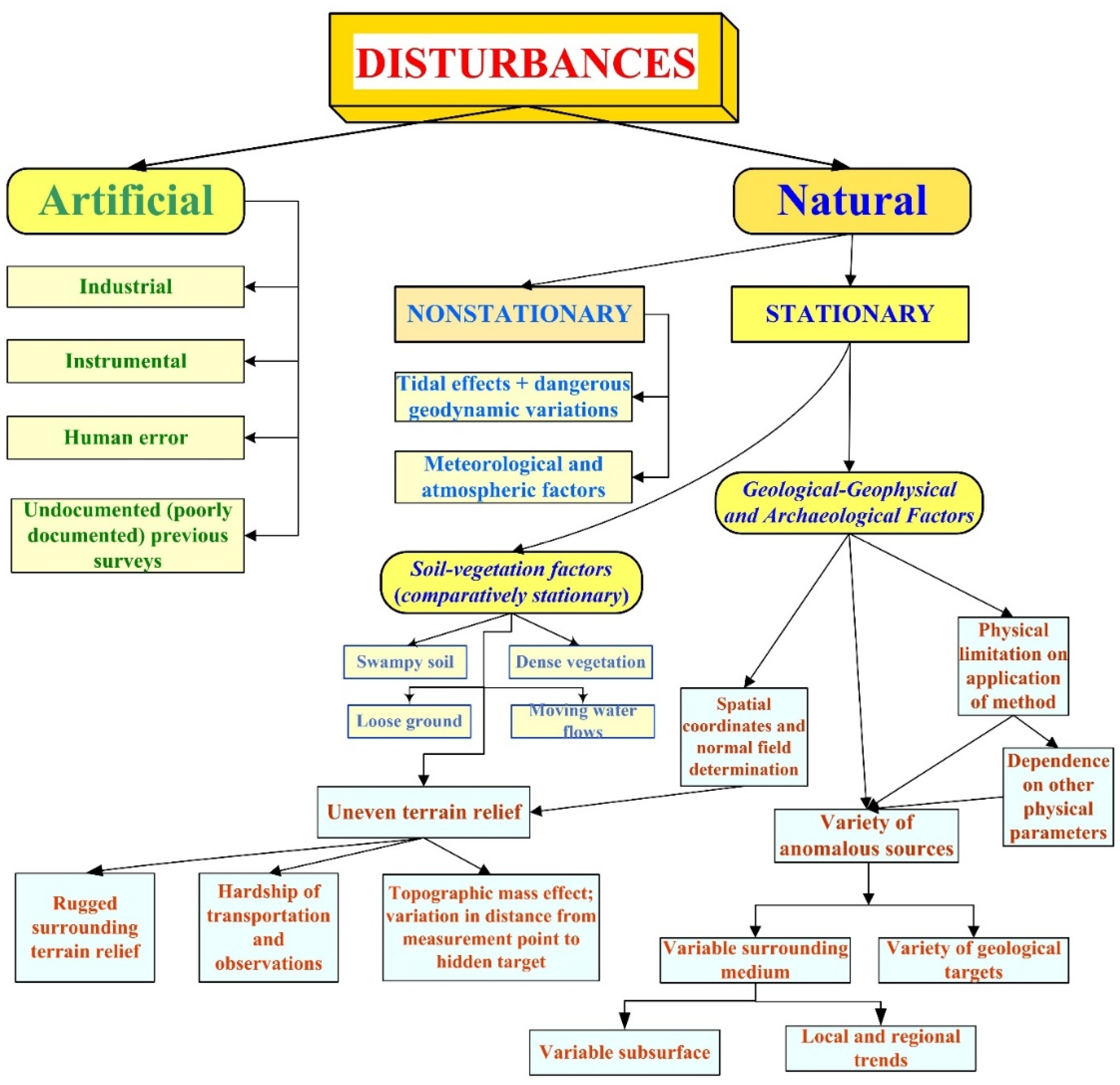
Figure 2.
Bouguer gravity anomalies computed from disturbing bodies with positive density contrast on uneven relief. (a) inclined smooth slope, (b) inclined complicated slope. (1) inclined profile, (2) horizontal profile, (3) anomalous body with a positive contrast density of 750 kg/m3, anomalies ΔgB, (4) on an inclined profile, (5) on a horizontal profile.
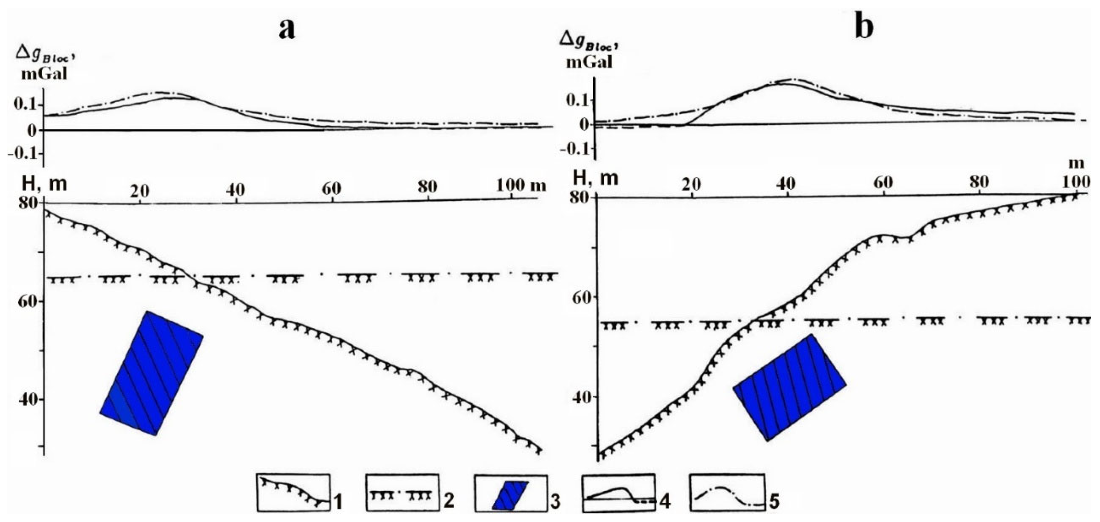
Figure 3.
Comparison of Bouguer gravity and vertical gradient anomalies. A: Bouguer gravity, B: vertical gradient gz (Wzz) computed for the base of 1.2 m, C: archaeological sequence.
Figure 3.
Comparison of Bouguer gravity and vertical gradient anomalies. A: Bouguer gravity, B: vertical gradient gz (Wzz) computed for the base of 1.2 m, C: archaeological sequence.
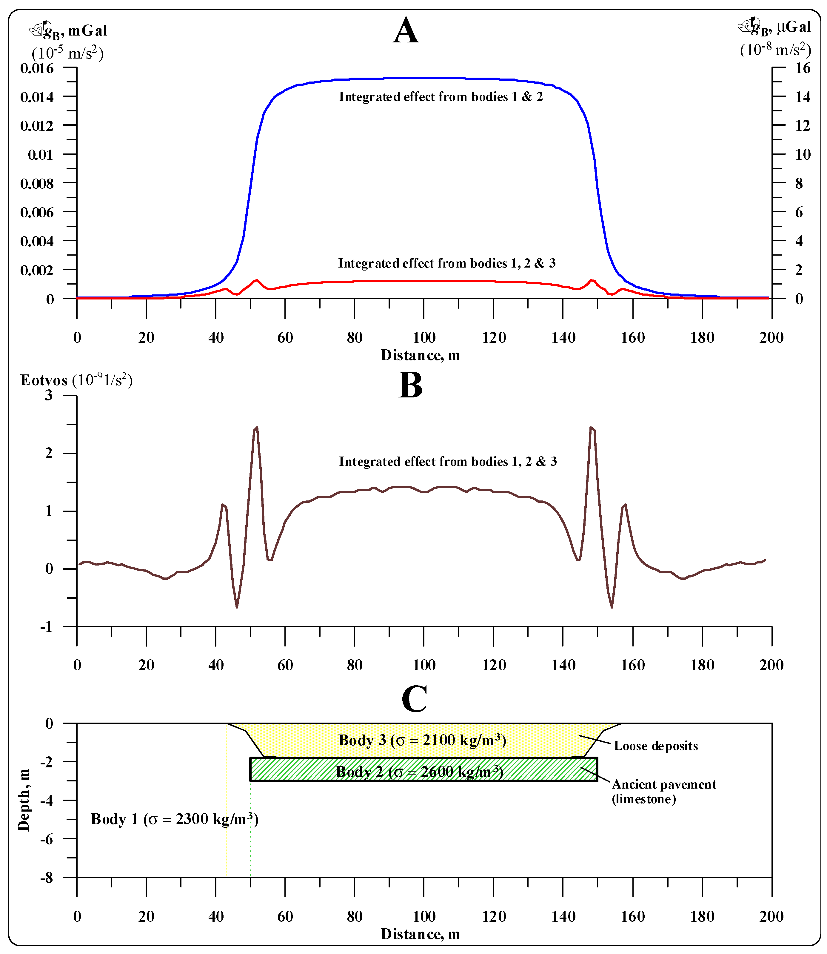
Figure 4.
Quantitative analysis of the gravity field from the buried archaeological cave under conditions of inclined relief.
Figure 4.
Quantitative analysis of the gravity field from the buried archaeological cave under conditions of inclined relief.
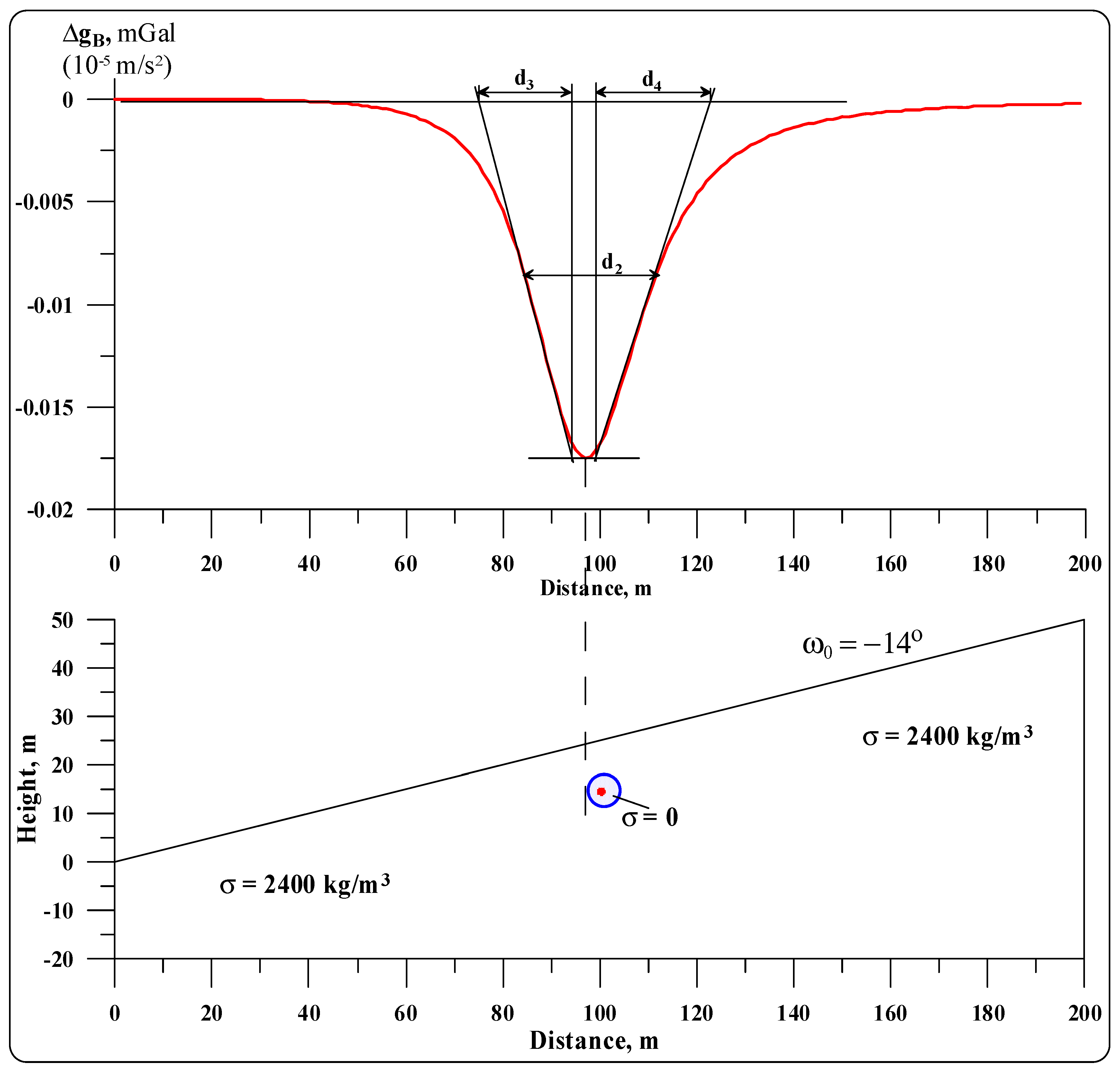
Figure 5.
Computing horizontal derivatives from models of two closely disposed underground caves. (A) Computed gravity curve, (B) Calculated first horizontal derivative of gravity field Δgx, (C) Calculated second horizontal derivative of gravity field Δgxx, (D) Physical-geological model.
Figure 5.
Computing horizontal derivatives from models of two closely disposed underground caves. (A) Computed gravity curve, (B) Calculated first horizontal derivative of gravity field Δgx, (C) Calculated second horizontal derivative of gravity field Δgxx, (D) Physical-geological model.
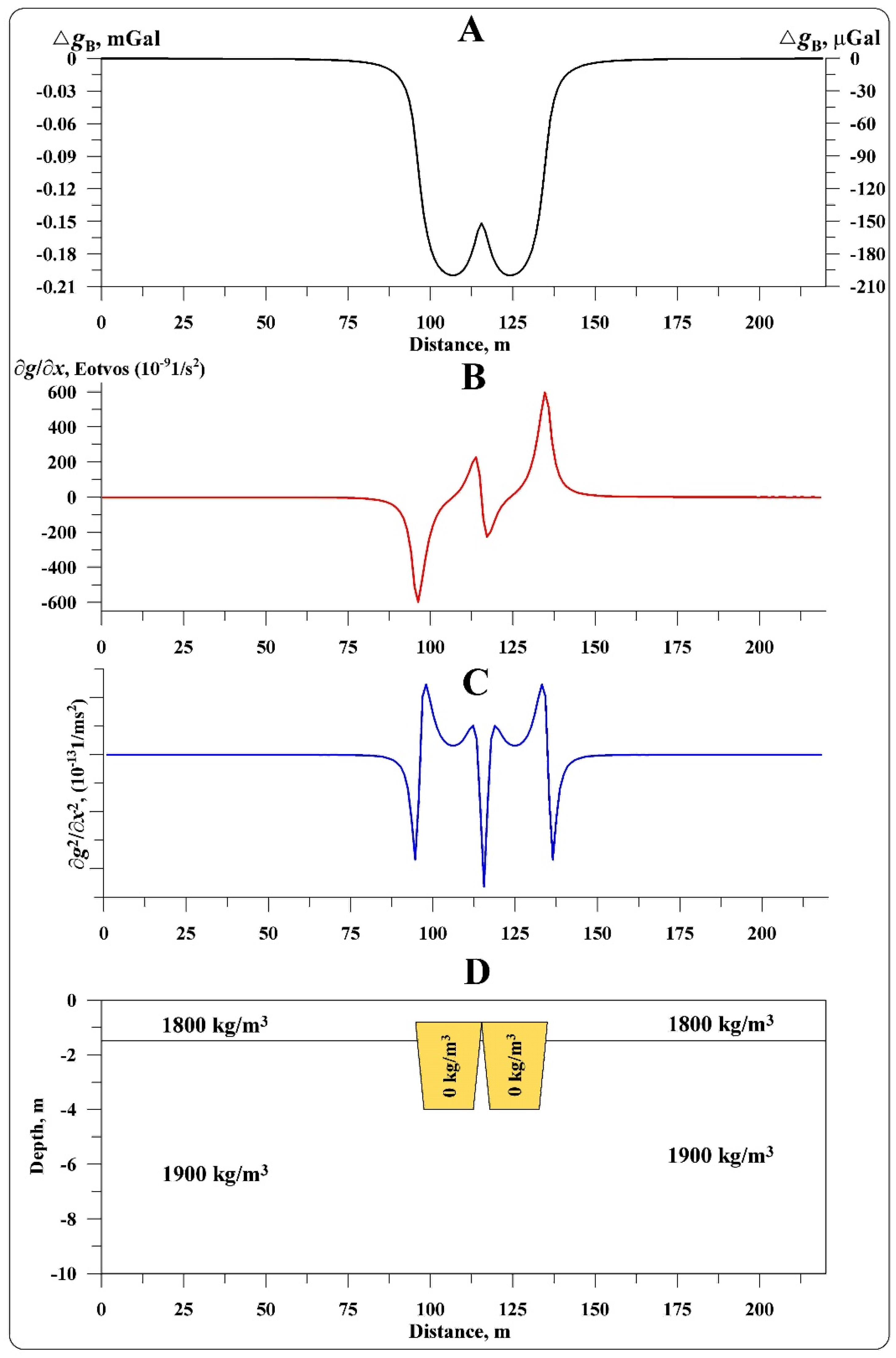
Figure 6.
Inverse problem solution for the model of sinkhole performed using methods developed for complicated environments. The red dot indicates the position of the center of the sphere.
Figure 6.
Inverse problem solution for the model of sinkhole performed using methods developed for complicated environments. The red dot indicates the position of the center of the sphere.
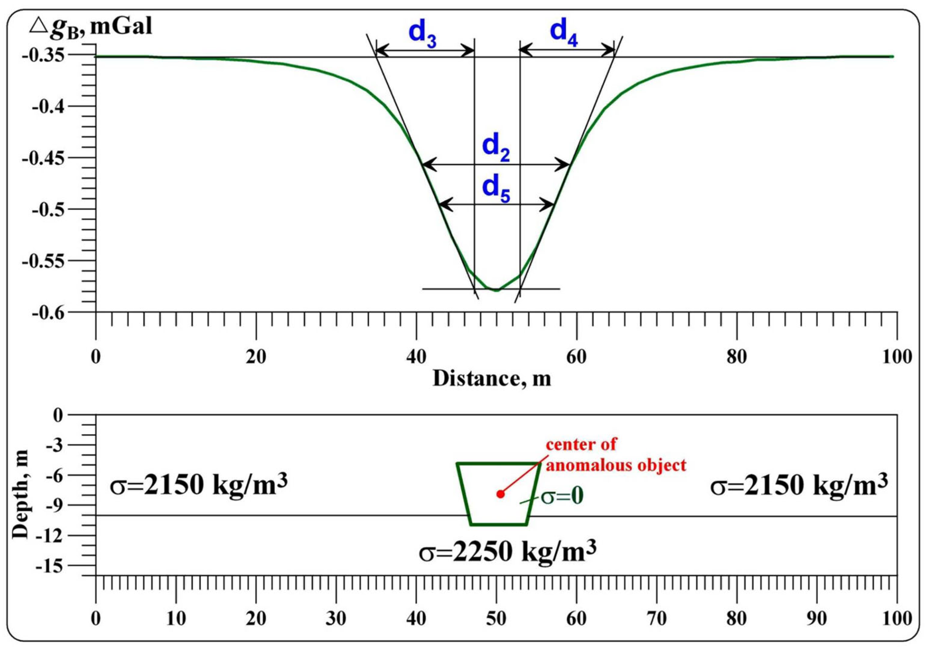
Figure 7.
Quantitative analysis of the gravity anomaly over the model of a thin horizontal bed (remains of the ancient Roman road). The blue crosses indicate the angle positions of the middle vertical thickness of the limestone road remain.
Figure 7.
Quantitative analysis of the gravity anomaly over the model of a thin horizontal bed (remains of the ancient Roman road). The blue crosses indicate the angle positions of the middle vertical thickness of the limestone road remain.
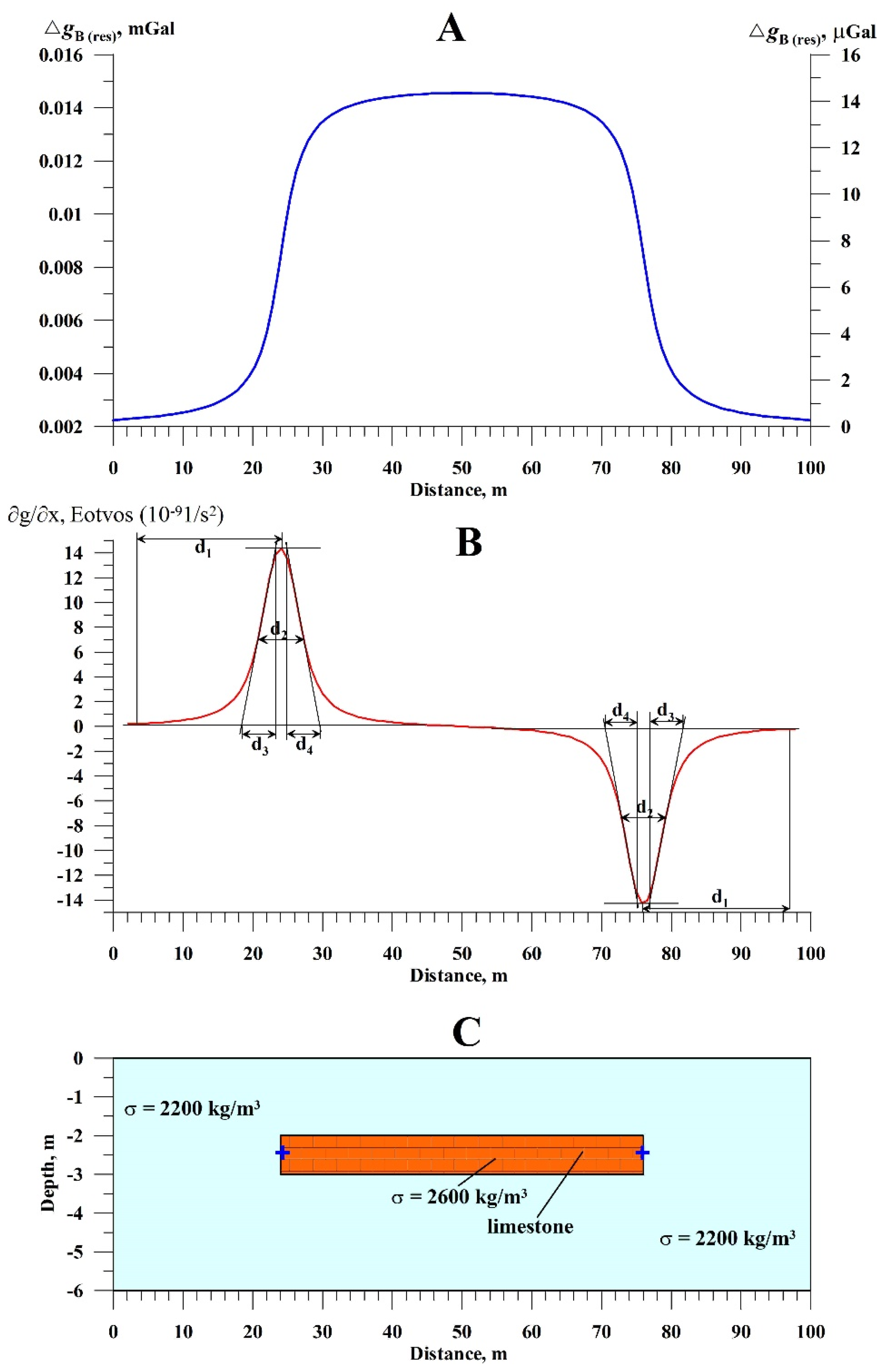
Figure 8.
Quantitative analysis of the gravity curve over the (initial data are after Padín et al. (2012)). The red circle with the dot shows the position of the HCC center (interpretation carried out by the author of this paper).
Figure 8.
Quantitative analysis of the gravity curve over the (initial data are after Padín et al. (2012)). The red circle with the dot shows the position of the HCC center (interpretation carried out by the author of this paper).
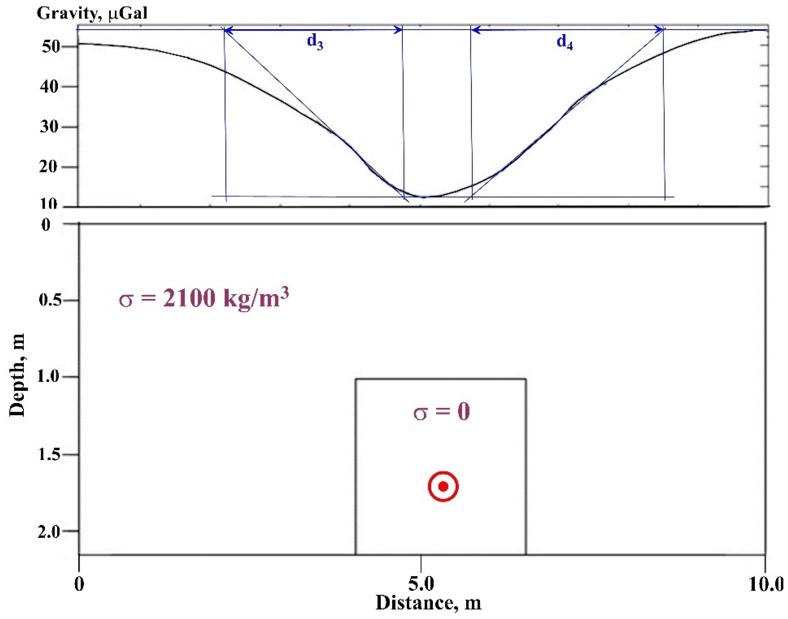
Figure 9.
Quantitative analysis of the gravity curve over the tunnel in the ancient Roman Amphitheater (initial data are taken from Di Filippo et al., 2005). The red circle with a dot indicates the position of the center of the HCC.
Figure 9.
Quantitative analysis of the gravity curve over the tunnel in the ancient Roman Amphitheater (initial data are taken from Di Filippo et al., 2005). The red circle with a dot indicates the position of the center of the HCC.
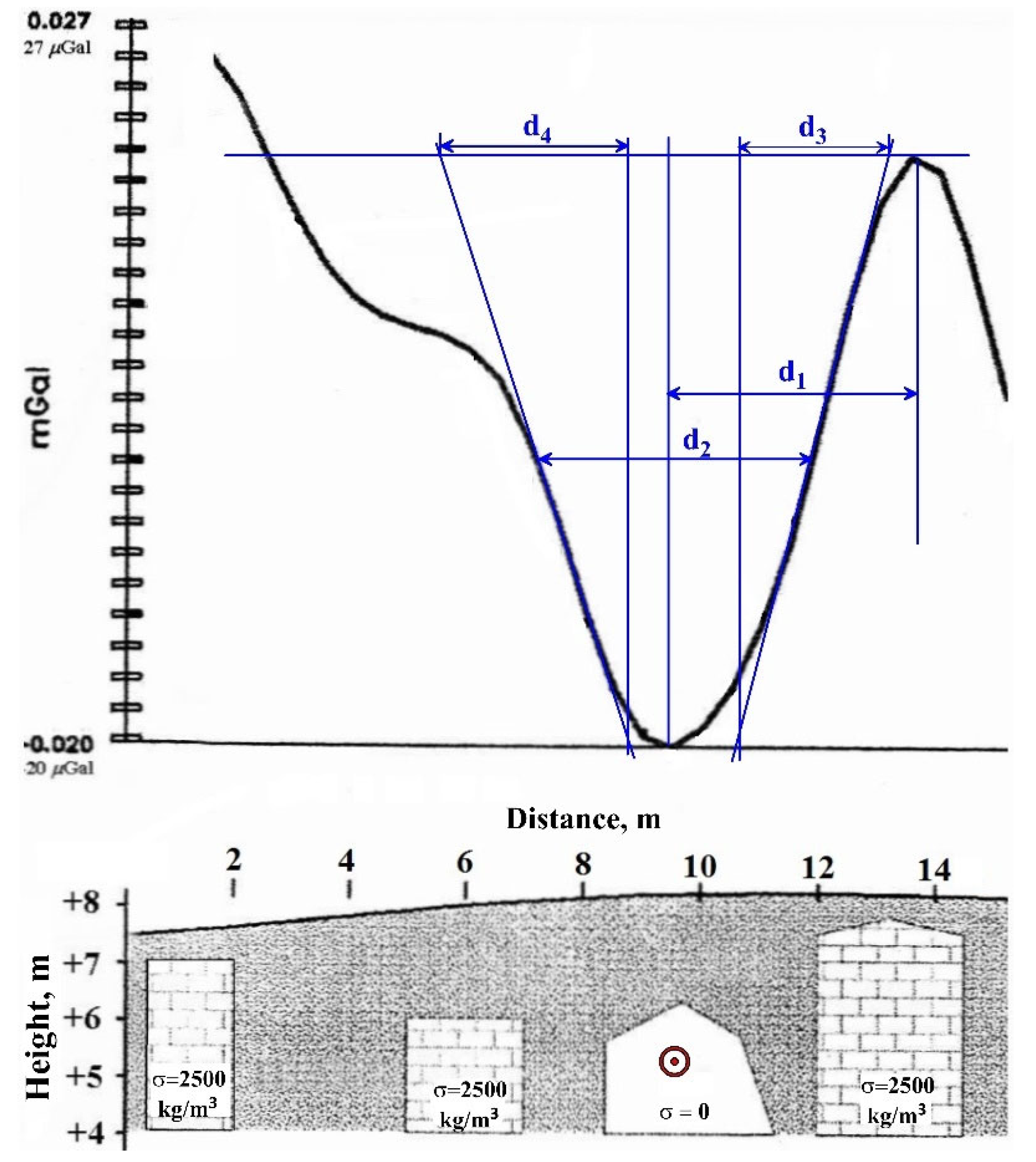
Figure 10.
Quantitative analysis of the gravity anomaly over the buried chamber in the Boden Vean, St. Anthony Meneage (Cornwall, UK) (the initial data are taken from Linford (1998)). The red circle with a dot indicates the position of the center of the HCC (author’s interpretation).
Figure 10.
Quantitative analysis of the gravity anomaly over the buried chamber in the Boden Vean, St. Anthony Meneage (Cornwall, UK) (the initial data are taken from Linford (1998)). The red circle with a dot indicates the position of the center of the HCC (author’s interpretation).
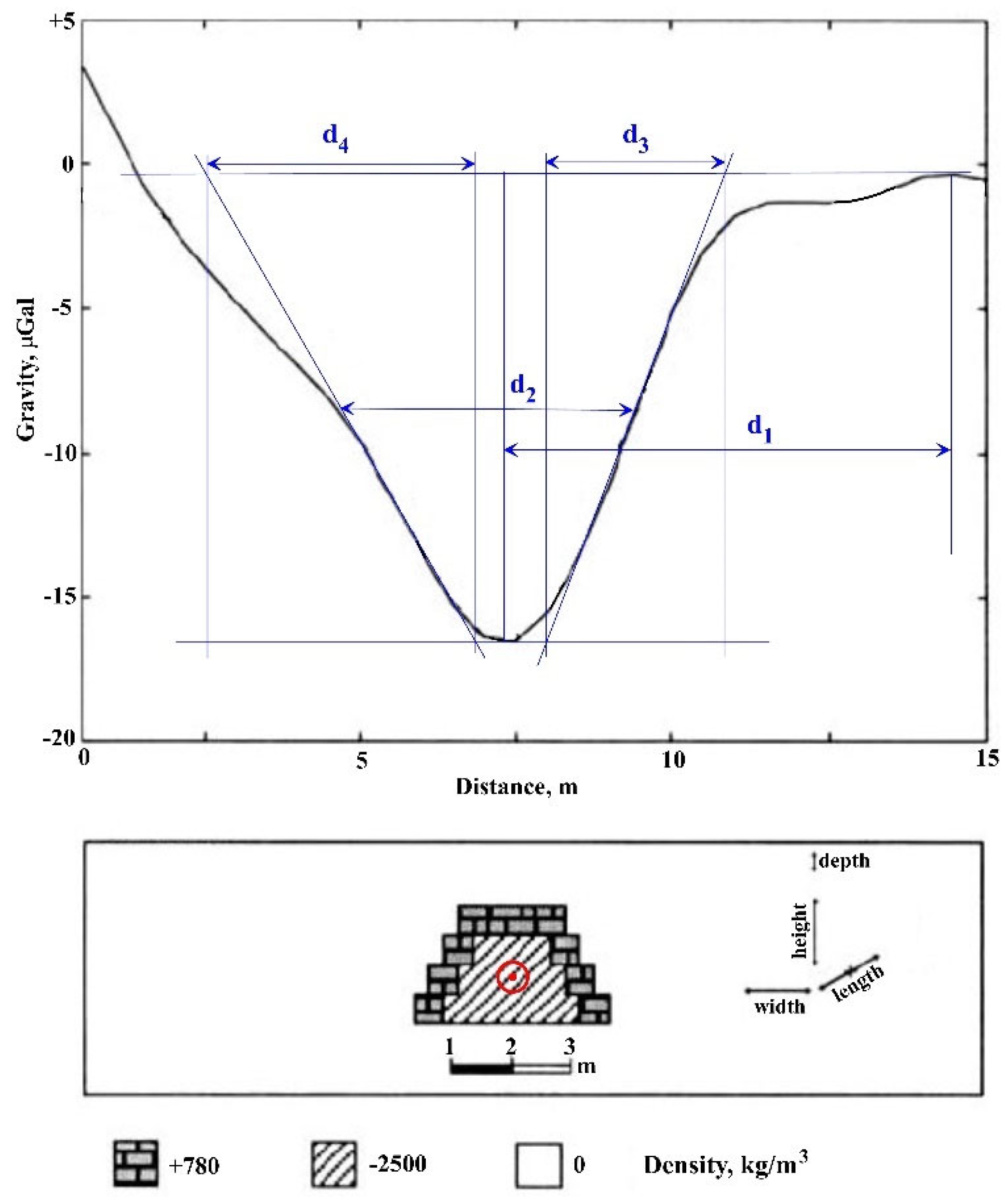
Figure 11.
Computing derivatives of the gravity potential for a horizontal polygonal prism.
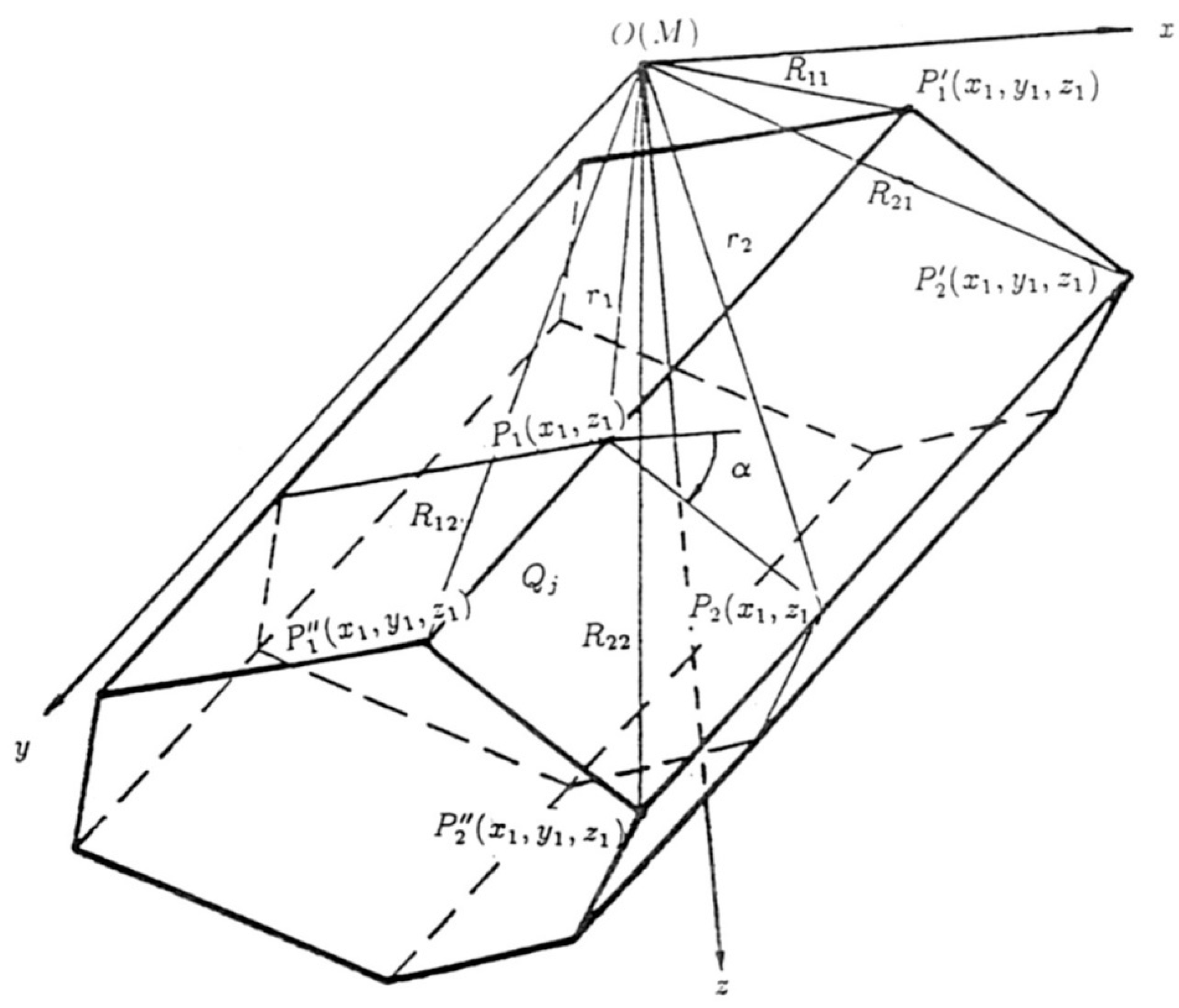
Figure 12.
Physical-geological model of a buried prehistoric cave and computed 3D gravity anomalies. (A) Location of projected profiles and disposition of buried cave (view over), (B) Computed gravity effects along profiles 1 – 5, (C) Geological-archaeological sequence (after Eppelbaum (2009), revised and supplemented).
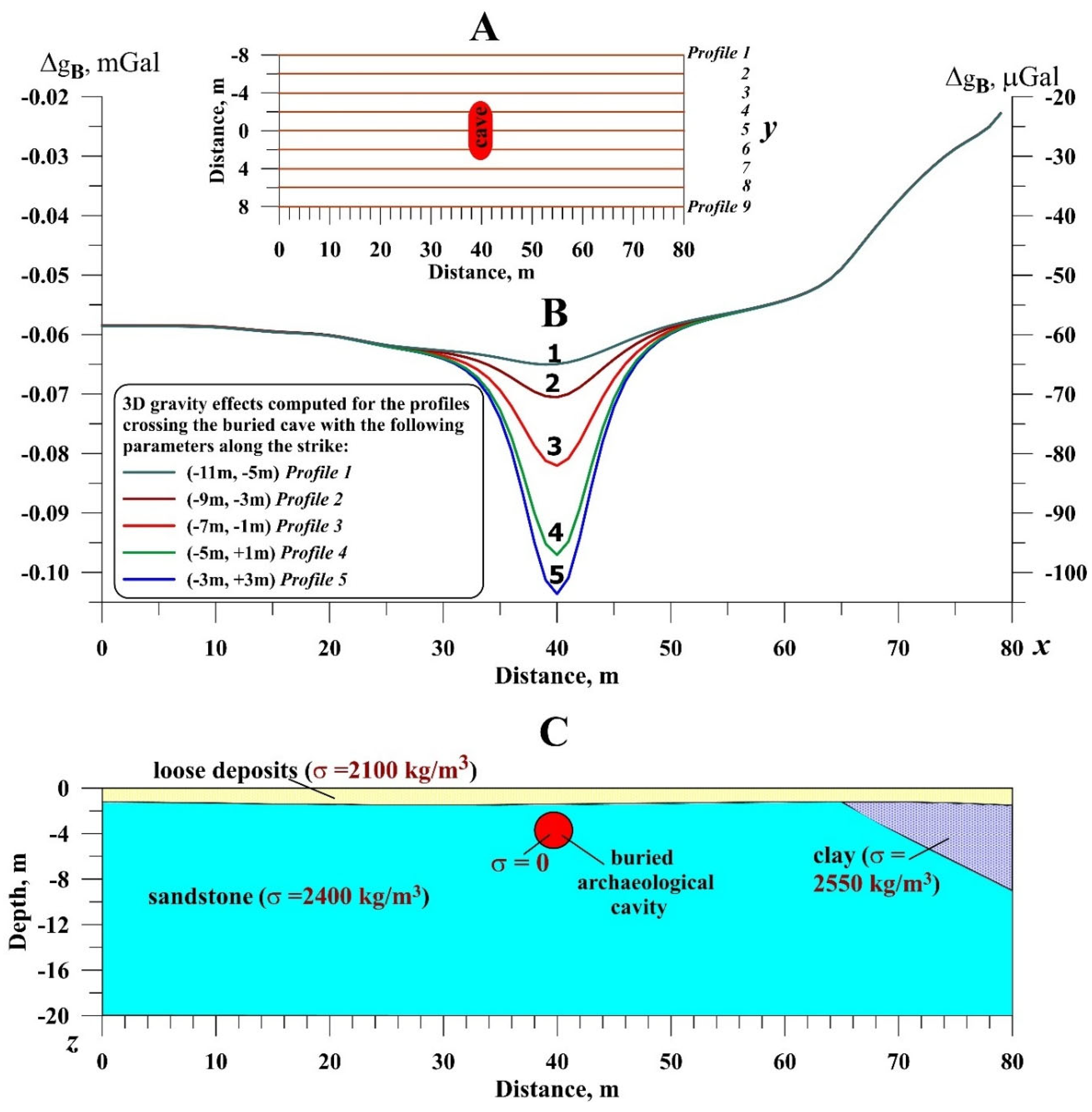
Figure 13.
3D gravity effects computed from a model of the buried furnace.
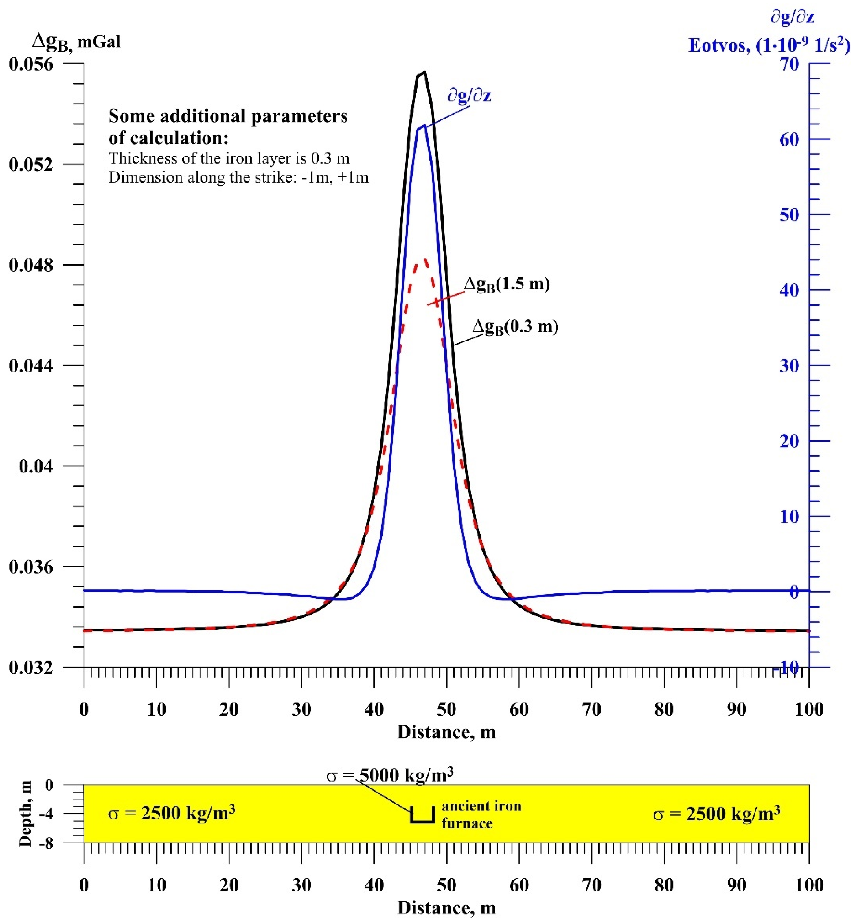
Figure 14.
3D gravity-magnetic effects from the initial PAM with the archaeological cavity and two geological layers (Model 1). Here σ is the density (kg/m3), and J is the magnetization (mA/m).
Figure 14.
3D gravity-magnetic effects from the initial PAM with the archaeological cavity and two geological layers (Model 1). Here σ is the density (kg/m3), and J is the magnetization (mA/m).
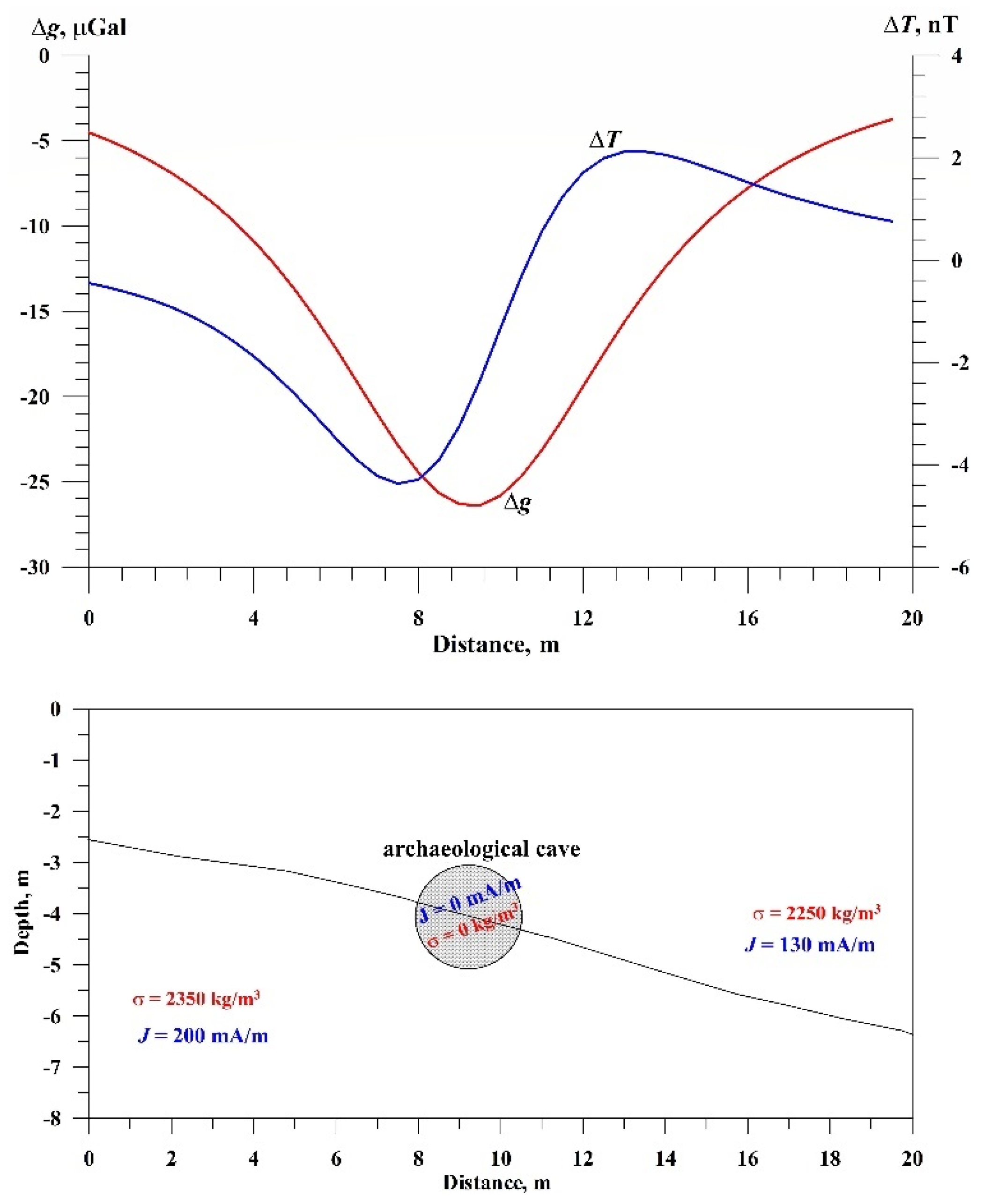
Figure 15.
3D gravity-magnetic effects from the PAM (one of the conventional geological sections) without the archaeological cavity (Model 5). Here σ is the density (kg/m3), and J is the magnetization (mA/m).
Figure 15.
3D gravity-magnetic effects from the PAM (one of the conventional geological sections) without the archaeological cavity (Model 5). Here σ is the density (kg/m3), and J is the magnetization (mA/m).
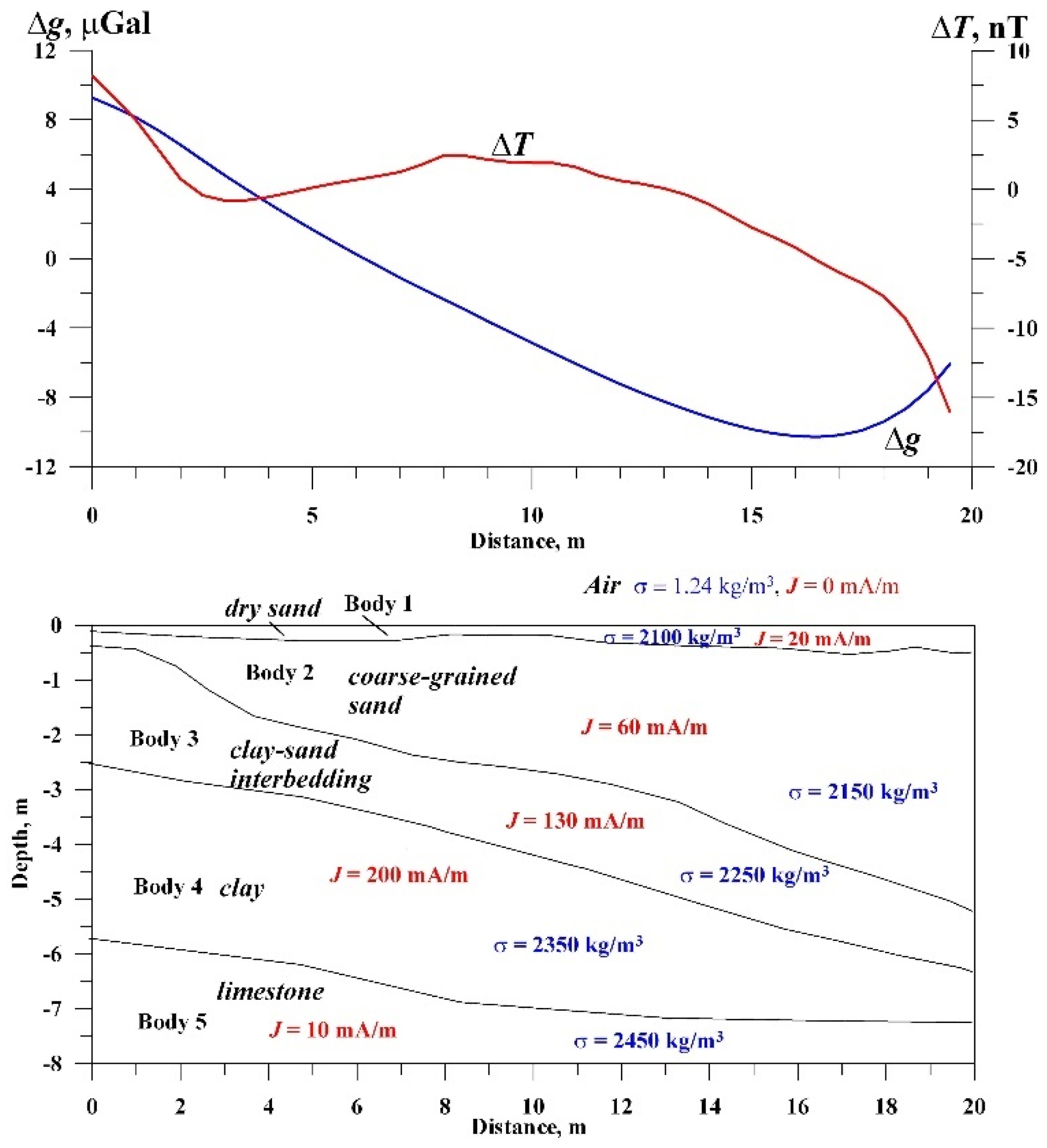
Figure 16.
3D gravity-magnetic effects from the PAM (one of the conventional geological sections) + the archaeological cavity (Model 32). Here, σ is the density (kg/m3), and J is the magnetization (mA/m).
Figure 16.
3D gravity-magnetic effects from the PAM (one of the conventional geological sections) + the archaeological cavity (Model 32). Here, σ is the density (kg/m3), and J is the magnetization (mA/m).
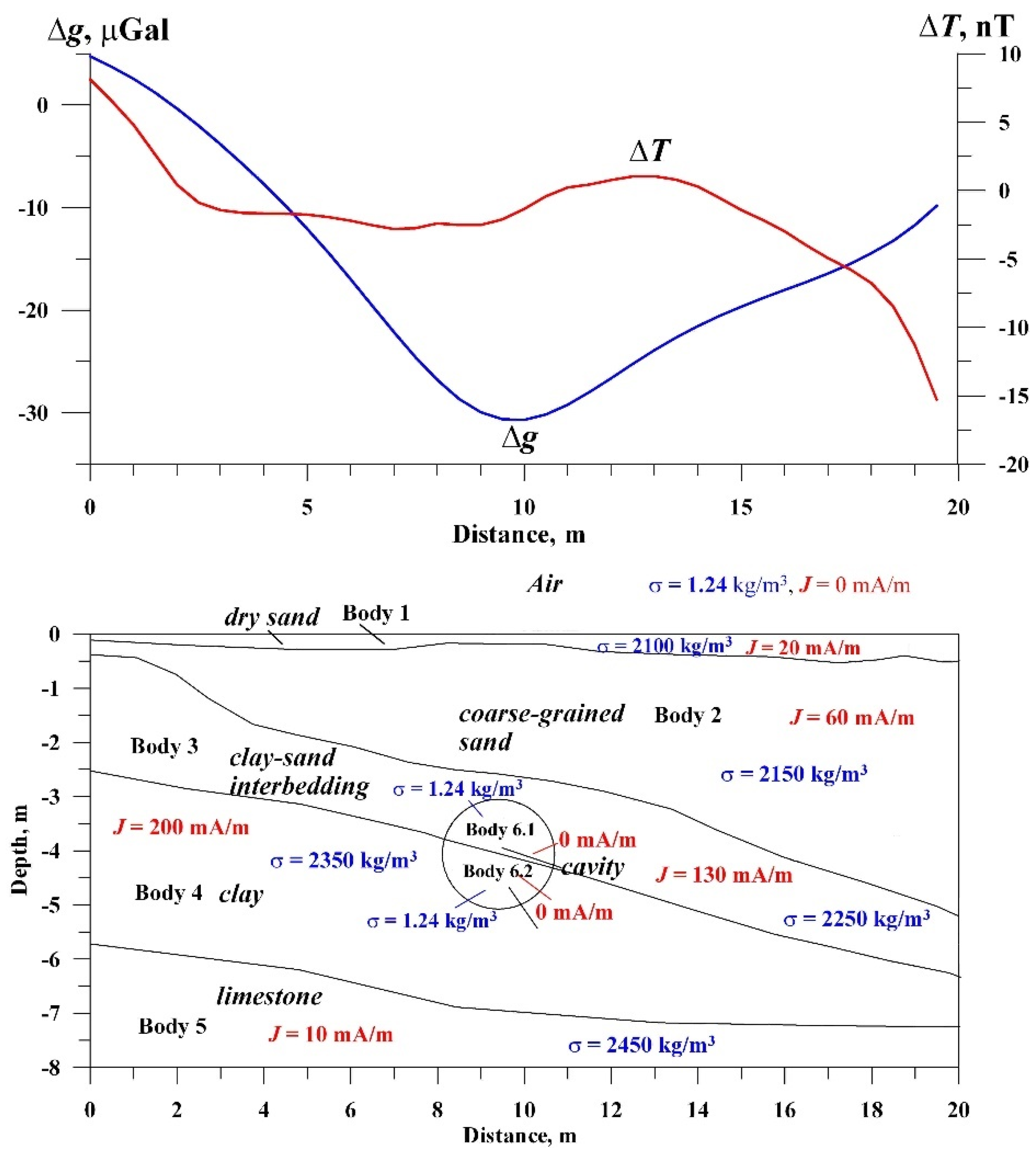

Table 1.
Comparison of some analytical expressions for magnetic and gravity fields.
| Field | Analytical expression | |
|---|---|---|
| Magnetic | Thin bed (TB) (3) |
Point source (rod) (4) |
| Gravity | Horizontal Circular Cylinder (HCC) (5) |
Sphere (6) |
Disclaimer/Publisher’s Note: The statements, opinions and data contained in all publications are solely those of the individual author(s) and contributor(s) and not of MDPI and/or the editor(s). MDPI and/or the editor(s) disclaim responsibility for any injury to people or property resulting from any ideas, methods, instructions or products referred to in the content. |
© 2025 by the authors. Licensee MDPI, Basel, Switzerland. This article is an open access article distributed under the terms and conditions of the Creative Commons Attribution (CC BY) license (http://creativecommons.org/licenses/by/4.0/).
Copyright: This open access article is published under a Creative Commons CC BY 4.0 license, which permit the free download, distribution, and reuse, provided that the author and preprint are cited in any reuse.


