Submitted:
26 June 2025
Posted:
27 June 2025
You are already at the latest version
Abstract
Efficient thermal management of lithium-ion batteries is crucial for electric vehicle safety and performance. This study investigates immersion cooling in serpentine channels for 18650 batteries, aiming to identify key factors affecting maximum battery temperature (Tmax) and pump power (Pw). A Box-Behnken experimental design is implemented with Computational Fluid Dynamics simulations to analyze responses Tmax and Pw. Five design variables are defined: partition length (Lp), battery charging/discharging rate (Crate), coolant volumetric flow rate (V), coolant inlet temperature (Tin) and ambient temperature (Tamb). Statistical significance is evaluated via Analysis of Variance. The results show that: Tin dominated Tmax, followed by Crate, V, and Lp. Significant interactions (V·Tin and V·Tamb) are observed. For Pw, V and V² show extreme significance, while Lp effects were minor. Interaction Lp·V was significant but secondary. After optimization to minimize Tmax, Tave and Pw, the optimal design values for Lp, Crate, V, Tin, and Tamb were determined to be 89.5 mm, 1.08 C, 0.51 LPM, 20 °C, and 25.62°C respectively. The corresponding optimized values are: Tmax = 22.87°C, Tave = 21.67°C, and Pw = 0.279 mW. Optimal thermal management requires prioritizing Tin control for temperature suppression and V regulation with non-linear compensation for energy efficiency.
Keywords:
response surface methodology
; battery thermal management
; CFD simulation
1. Introduction
The battery is one of the core components of a pure electric vehicle. At present, the power batteries of electric vehicles mainly include supercapacitors, nickel-based batteries, lead-acid batteries, lithium-ion batteries, zinc-air batteries, etc. Among them, lithium-ion batteries have become the preferred solution for electric vehicle manufacturers due to their high energy density, light weight, and long service life. However, the performance, lifespan and safety of lithium-ion batteries are very sensitive to temperature. An efficient battery thermal management system should ensure that the battery operates within the optimal working temperature range (15-35 °C) [1,2]and make the temperature distribution on the battery surface uniform. If the temperature of lithium-ion batteries exceeds 50°C, the charging efficiency and service life will be greatly reduced [3]. In the temperature range of 70-100°C, lithium-ion batteries may triggering thermal runaway and other safety accidents [4].
At present, the most commonly used thermal management methods in lithium-ion batteries include air cooling, liquid cooling, phase change materials (PCMs) and heat pipe cooling technologies [5]. The air cooling technique pumps ambient air to purge the battery module to accelerate the heat dissipation. It has the characteristics of simple structure, easy implementation and relatively low cost, but the cooling efficiency is low. Akinlabi and Solyali [6] reviewed the air-cooling battery thermal management systems, and concluded that it is difficult to control the temperature of high-energy-density lithium batteries by air-cooling battery thermal management system (BTMS). The PCMs cooling system is a passive cooling method, and the PCMs used usually has a large latent heat of fusion and an ideal melting point, and can store a large amount of heat generated during the charging and discharging process of the battery. However, the PCMs usually have low thermal conductivity and lead to poor thermal propagation. The PCMs should be modified[7,8,9] or added with other additives [10,11], and used in conjunction with other cooling methods [12,13,14]. Similar to the phase change material cooling system, heat pipe cooling usually needs to be used in combination with other cooling methods [15,16,17], and the heat transfer performance of the heat pipe will be reduced when the vehicle is affected by shock and vibration.
The liquid cooling system has gradually become the hotspot of BTMS. According to the contact type between the coolant and the batteries, it is usually divided into indirect liquid cooling (ICLC) and direct liquid cooling (DCLC, also called as immersion cooling) [18]. Indirect contact liquid cooling usually uses water or a mixture of water and ethylene glycol as the coolant. The coolant flows in channels of pipes, cold plates or water jackets, and removes the heat generated by the battery. Due to the electrical conductivity of the coolant, the indirect cooling system needs to be well sealed to prevent liquid leakage from causing a short circuit. At the same time, the thermal contact resistance between the metal separator and the battery needs to be considered. Although the indirect cooling system has good heat dissipation capacity, the structure of the system is relatively complex, the whole system is very bulky, expensive, and the maintenance cost increases. In the early days of direct contact liquid cooling, deionized water, silicone oil, mineral oil, and refrigerants were commonly used as coolants[19]. Although liquid has a high thermal conductivity compared with air, which can effectively reduce the maximum temperature of the batteries, the direct contact liquid cooling system still greatly relies on the liquid cooling arrangement to enhance the convective heat transfer coefficient, thereby improving the overall temperature uniformity of the battery pack.
In recent years, the immersion cooling system for power battery thermal management has become a new research hotspot. The battery is immersed in a dielectric coolant. Unlike the indirect liquid cooling system, the immersion cooling system has no contact thermal resistance, smaller volume, higher cooling efficiency, and more uniform temperature distribution. To prevent short circuits and electrochemical corrosion between the battery and the working fluid, the coolant should be selected to have insulation properties, non-toxicity, chemical inertness, high thermal conductivity, and flame-retardant characteristics [20,21]. Such fluids typically offer superior thermal performance for BTMS. Nelson and colleagues [22] developed a battery module comprising 12 serially connected cells, incorporating 1 mm wide flow channels filled with silicone oil between adjacent cells. Their experiments demonstrated that silicone oil, serving as a thermal medium, offers significantly better heat dissipation performance than air cooling. Karimi et al. [23] carried out a comparative assessment of water, silicone oil, and air as cooling media, showing that liquid-based cooling can effectively keep battery temperatures within an acceptable operational range, although minor internal temperature variations may still occur. Hirano et al. [24] explored the use of 3M’s Novec7000 for immersion cooling applications. The results indicated that when the battery undergoes 20C high-rate charge and discharge cycles, submerging it in Novec7000 successfully maintains maximum battery temperature Tmax at a stable 35°C. Tan et al. [25] utilized HFE-6120 as the working fluid, and conducted CFD simulations to analyze its key operational parameters in DCLC system. Satyanarayana et al. [26] compared the immersion cooling effectiveness of mineral oil and terminal oil under varying discharge rates. Their findings revealed that low-viscosity mineral oil is more efficient in managing Tmax, achieving a reduction of up to 49.16% in Tmax compared to natural air convection cooling. Patil et al. [27] investigated the direct cooling performance of Li-ion batteries using dielectric fluid immersion cooling combined with tab cooling. By inserting baffles, the disturbance and residence time of the coolant are increased. The results demonstrated significantly improved thermal management, with up to a 46.8% reduction in maximum tab temperature and better overall pack performance compared to conventional cooling methods. Wu et al. [28] compared single-phase and two-phase liquid cooling systems for large lithium-ion batteries, showing that the single-phase system with deionized water and copper foam provides superior thermal performance, achieving lower temperatures and better uniformity during high-rate discharge. Choi et al. [29] proposed a hybrid immersion-cooling structure with one pass partition and graphite fins. The performance of the structure was investigated with variations in key design parameters such as flow direction, battery spacing, pass partitions, and thermal conductive materials. The results show that, compared to conventional structures, this hybrid immersion structure achieves a maximum temperature reduction of 6.7 °C and a temperature difference reduction of 3.0 K under nearly the same weight condition. Zhao et al. [30] developed a hybrid battery thermal management system combining direct liquid cooling with forced air cooling. A jacket was designed outside the battery, with liquid coolant filled between the battery case and the jacket to achieve direct cooling, while air cooling was applied externally. The effects of gap spacing between the battery and liquid-cooling jacket, number of cooling pipelines, liquid flow rate, and fan position on cooling performance were analyzed through numerical simulation. Febriyanto et al. [31] investigated the thermal performance of a Serpentine Channel Immersion Cooling (SCIC) system. The results showed that increasing the coolant flow rate enhances the heat transfer coefficient and reduces battery surface temperature, with a notable balance between heat dissipation and pumping power at 1 LPM (liters per minute).
The above-mentioned studies demonstrate that improvements in the single-phase immersion cooling performance of batteries are mainly achieved through the use of higher-performance coolants or the optimization of flow channel structures. While structural optimization of flow channels has proven effective in enhancing heat dissipation, there remains a significant lack of quantitative research on the relationships between channel design parameters, operational parameters, and thermal response indicators—particularly the maximum battery temperature Tmax and pump power consumption Pw. Current research is largely confined to experimental validations or simulation trials based on discrete parameter values, with no universally applicable mathematical correlation model yet established. In this study, 18650-type lithium-ion batteries are selected as the research subject, and HFE-7100 was chosen as the immersion coolant. A battery thermal management model incorporating a serpentine channel configuration was developed using the ANSYS Fluent computational fluid dynamics platform. The focus is on investigating the impact mechanisms of key factors such as partition length, coolant flow velocity, and ambient temperature on thermal performance. To overcome the limitations of traditional single-variable analysis methods, this study employed Response Surface Methodology (RSM) to construct a quadratic polynomial regression model. Experimental conditions were designed using the Box-Behnken Design (BBD) approach, enabling systematic quantification of the contributions of each design variable and their interactions on Tmax and Pw. This mathematical model accurately captures the nonlinear variation patterns of thermal responses under multi-parameter coupling conditions, providing a solid theoretical foundation for the optimized design of immersion cooling systems.
2. Methodology
2.1. Physical Model
The battery module’s geometric design is derived from literature [31], as shown in Figure 1. It uses a 290 mm × 120 mm × 75 mm rectangular housing. Twenty-four 18650 LiFePO4 batteries are connected in series. The individual battery cell model has dimensions of 18 mm diameter × 65 mm height, represented by a cylindrical approximation. The spacing between adjacent columns is 24 mm, while the spacing between rows is 31 mm. The layout follows a six-loop serpentine-channel pattern with 4 batteries per row. All batteries maintain identical electrode orientation. Partitions physically separate battery groups. The module provides 78.6 V nominal voltage. Table 1 summarizes parameters of 18650-type batteries, while Table 2 lists key thermophysical properties of HFE-7100 coolant (data sourced from [31]).
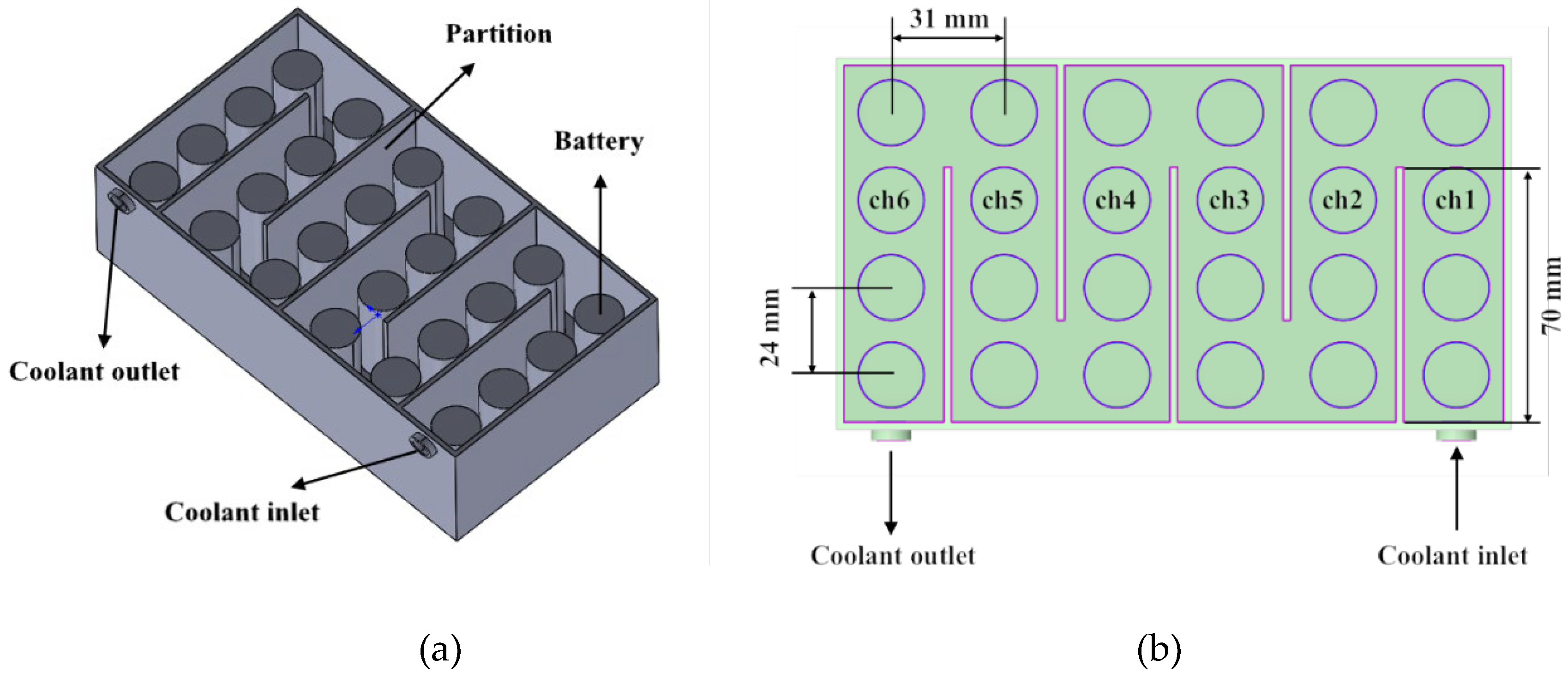
Figure 1.
Schematic diagram of the battery module: (a) Three-dimensional view of battery holder design; (b) Flow channel configuration.
Figure 1.
Schematic diagram of the battery module: (a) Three-dimensional view of battery holder design; (b) Flow channel configuration.

Table 1.
Technical parameters of lithium-ion battery [31].
Table 1.
Technical parameters of lithium-ion battery [31].
| Parameter | Specification | Parameter | Specification |
| Type | LiFePO4 | Max Charge Current | 1C |
| Nominal Capacity | 1800 mAh | Weight | 46±1 g |
| Minimum Capacity | 1775 mAh | Diameter | 18 mm |
| Nominal Voltage | 3.2 V | Height | 65 mm |
| Internal Resistance | 30 mΩ | Battery arrangement | 24S |
| Discharge Cut-Off Voltage | 2.5 V | Total Nominal Voltage | 76.8 V |
| Max Charge Voltage | 3.65 V |
Table 2.
Thermophysical properties of HFE-7100 [31].
Table 2.
Thermophysical properties of HFE-7100 [31].
| Properties | Values | Unit |
| Boiling point | 334.15 | K |
| Specific heat | 1170 | J/(kg⋅K) |
| Latent heat vaporization | 112 | kJ/kg |
| Thermal conductivity | 0.068 | W/(m⋅K) |
| Liquid density | 1418.64 | kg/m3 |
| Vapor density | 0.98 | kg/m3 |
| Kinematic viscosity | 3.008×10⁻⁷ | m2/s |
2.2. Governing Equations
Some assumptions are made here to simplify the problem:
- (1)
- Constant physical properties are maintained for both liquid coolant and battery components.
- (2)
- Perfect interfacial contact is established between solid and fluid domains (no-slip boundary condition).
- (3)
- Incompressible flow is adopted for coolant.
- (4)
- Buoyancy effects on fluid flow are excluded from the simulation.
- (5)
- Thermal radiation is omitted in the heat transfer simulation.
For the HFE-7100 liquid, the continuity equation can be written as:
where ρl is the density of the fluid, u is velocity component and t is time.
Momentum equation of single-phase HFE-7000 flow:
where p is the pressure, µeff is the effective viscosity and has the form of:
where µ is molecular viscosity, µt is turbulent viscosity. The turbulent viscosity µt is directly related to the turbulent kinetic energy k and the dissipation rate ε:
The transport equations in k-ε model are shown as:
where Gk is the production of turbulence kinetic energy. Values of the constants in the k-e equations are given as follows: Cμ=0.09, C1=1.44, C2=1.92, σk=1.0, σε=1.3.
The energy conservation equation of the coolant is:
The energy conservation equation of the battery cell is expressed as:
where ρs, Cp,s, and T are the battery material density, specific heat capacity, and temperature, respectively. λs is the thermal conductivity of the battery. The heat source term, Sb, is the volumetric heat generation rate in the battery cell which can be divided into reversible heat and irreversible heat according to their origins, and can be presented as:
where I represents the current, Vt represents the voltage during operation, U represents the voltage when the circuit is open, T represents the temperature of battery, and ∂U/∂T represents the coefficient of entropy.
Discharge current I at any discharge rate can be determined by multiplying the Crate by the battery’s nominal capacity:
The ideal pump power is calculated as:
where Pw is pump power, ΔP is the pressure drop between the coolant inlet and outlet, V is the volumetric flow rate of the coolant.
2.3. Solution Strategy
2.3.1. Boundary Conditions
In this study, the coolant velocity is specified as an input parameter, with the inlet of the computational domain defined as a velocity inlet boundary. So, the velocity inlet boundary condition is applied, with the flow direction orthogonal to the inlet plane:
On the outer surfaces of the battery module, a no-slip wall boundary condition is applied, and a convective heat transfer coefficient h of 20 W/(m2·K) is assigned to model heat dissipation. Tamb is the ambient temperature, and satisfies the following formula:
At the outlet, the boundary is defined as an outflow condition to accommodate variable flow rates:
At the fluid-solid interface, continuity of temperature and heat flux is enforced to ensure energy conservation:
2.3.2. Mesh Independence Check
To ensure the reliability of numerical simulations for battery immersion cooling, a comprehensive grid independence study was conducted by systematically refining the mesh resolution from coarse to medium and fine, as depicted in Table 3. The results indicate that the maximum battery temperature under the medium grid density deviates by less than 0.86% compared to the finest mesh, while temperature gradients exhibit a maximum deviation of 1.57%. The detailed mesh structure of the computational domain is illustrated in Figure 2. Given these results, the medium grid configuration was ultimately selected as a balance between computational efficiency and solution accuracy, ensuring y+ values below 5 in boundary layers. The simulations were performed using a pressure-based solver with the pressure correction algorithm for pressure-velocity coupling. The Navier-Stokes equations were solved via a SIMPLEC algorithm, while the convective and diffusive terms in the energy equation were discretized using a second-order upwind scheme. Convergence criteria were set to 10−4 for continuity and momentum equations and 10−6 for energy equations throughout all simulations.
2.4. Response Surface Design
The Response Surface Method (RSM) is a statistical experimental design and data analysis technique used to systematically study the quantitative relationship between multiple influencing factors and a response variable. By constructing a mathematical model (such as a quadratic polynomial equation), RSM efficiently identifies the effects of key parameters on the output while minimizing the number of required experiments. Its main advantages include significantly reducing experimental costs, avoiding the high resource consumption associated with full factorial designs, and enabling precise determination of optimal operating conditions. Additionally, it allows for accurate prediction of response values under various conditions, thereby enhancing both the efficiency and reliability of the experimental outcomes. In this study, RSM was employed to establish the nonlinear response relationships between operational parameters (e.g., flow rate, coolant temperature), battery arrangement parameters (e.g., partition length), and battery temperature distribution, providing a theoretical foundation and practical guidance for optimizing thermal management strategies.
In this study, the partition length (Lp), battery discharge rate (Crate), coolant volumetric flow rate (V), coolant inlet temperature (Tin), and ambient temperature (Tamb) were selected as design variables, while the battery maximum temperature (Tmax), average temperature (Tave), and pump power (Pw)were chosen as response values. A response surface methodology with five factors at three levels and two response values was employed. The coding rule was defined as follows: 0 for the center level, -1 for the minimum level, and 1 for the maximum level. The coded matrix based on the Box-Behnken Design (BBD) is presented in Table 4.
Using Design expert 13.0 software and following the design principles of the BBD, a total of 46 experimental runs, including six center points, were designed for the five factors at three levels. The design scheme and results of the BBD experiments are summarized in Table 5.
3. Results and Discussion
3.1. Model Validation
Prior to analyzing the impact of battery design parameters on thermal behavior, validating the accuracy of the numerical model is essential. This study uses experimental data from Febriyanto et al. [31] to verify the numerical model. Figure 3 presents a comparison between the simulated data and the experimental results from Ref. [31]. Figure 3a shows the comparison of temperature values at the observation points across the six channels under 1C and 2C discharge rates. As can be observed from the figure, the simulated temperatures at all observation points are in good agreement with the experimental measurements. Under the 1C discharge rate, the maximum absolute error between the simulated and experimental values is 0.7 °C, with a corresponding relative error of 2.82%. Under the 2C discharge rate, the maximum absolute error is 1.0 °C, and the maximum relative error is 3.71%. Figure 3b compares the average temperatures across all six observation points between the simulation and experiment. It can be seen that, under the same discharge rate, the average temperature decreases with increasing coolant flow rate, and the simulated results align well with the experimental data. The maximum error occurs under the 1C discharge rate with a coolant flow rate of 0.5 LPM, where the absolute error is 0.58 °C, corresponding to a relative error of 2.17%. The results demonstrate a high degree of consistency between the numerical simulation outcomes and the experimental data, not only validating the model’s capability to accurately predict the actual temperature distribution but also confirming its reliability as a foundation for further investigations.
3.2. Analysis of Variance
3.2.1. ANOVA of Battery Temperature
Table 6 is the ANOVA results for Tmax after backward elimination. The ANOVA results indicate that the constructed quadratic polynomial model possesses extremely high statistical significance. The F-value is a ratio obtained by dividing the model mean squares by the error of mean squares. It is a statistic used to test the overall significance of the model. A higher F-value indicates that the model explains a substantial portion of the variability in the data, rather than variations caused by random noise. This helps determine whether the independent variables significantly affect the dependent variable. The p-value is the probability used to decide whether to reject the null hypothesis. The null hypothesis typically states that all model coefficients are equal to zero (i.e., the model has no explanatory power). A smaller p-value suggests that the observed data (or more extreme results) would be less likely to occur under the null hypothesis. Generally, if the p-value is less than 0.05, the result is considered statistically significant. In Table 6, the model’s F-value reached 4768.12, significantly greater than 1, with a corresponding p-value less than 0.0001. This demonstrates that the model’s ability to predict Tmax is statistically very significant. According to the statistical standards of response surface methodology (RSM), a model p-value < 0.01 indicates good fitting accuracy, allowing this response surface approximation model to be employed in subsequent optimization design. In this study, the p-values for all main effects and interaction effects were significant (all < 0.01 or < 0.05), further confirming the model’s validity.
The ANOVA results reveal the significance and relative importance of each factor’s influence on Tmax. Based on the magnitude of the F-values, the factors are ranked in descending order of influence on Tmax as follows: Tin > Crate > V > Lp > Tamb. Tin had the highest F-value (48033.91) and the largest Sum of Squares (336.81), indicating it is the most significant factor affecting Tmax, with a contribution far exceeding that of other variables. Regarding interaction effects, the interactions V·Tin and V·Tamb were the most significant (F=26.37), followed by Crate·V (F=17.47). The existence of these interaction terms indicates that the effects of the factors on Tmax are not independent; rather, they exhibit complex synergistic or antagonistic effects. For instance, the significant V·Tin and V·Tamb interactions suggest that optimizing the level of V requires simultaneous consideration of the levels of Tin and Tamb to achieve the optimal Tmax value.
The R2 value measures the proportion of total variation explained by the model. Ranging from 0 to 1, a value closer to 1 indicates a better fit of the model to the data. However, R2 has a limitation: it tends to increase (or at least not decrease) as more independent variables are added to the model, even if these variables are unrelated to the response variable. This may lead to overfitting. To address this limitation of R2, the adjusted R2 is introduced. It accounts for the number of independent variables in the model by imposing a penalty for each additional variable. Consequently, adjusted R2 increases only if a newly added variable genuinely enhances the model’s explanatory power. This makes it a more reliable metric for comparing models with different numbers of independent variables. Predicted R2 evaluates the model’s predictive capability. Based on cross-validation principles, it partitions the dataset, trains the model on one subset, and tests its predictive accuracy on the remaining subsets. A higher predicted R2 indicates better performance on unseen data. If predicted R2 is significantly lower than R2, it suggests potential overfitting. The S-value represents the average deviation between observed and predicted values. As the standard deviation of model residuals, it estimates the uncertainty of predictions. Generally, a smaller S-value implies closer alignment of predictions with actual observations, reflecting higher model precision. For a model to demonstrate high fitting accuracy and robust predictive capability, the following conditions should be met: R2 and adjusted R2 are both high and relatively close, indicating strong explanatory power without over-reliance on redundant variables. Predicted R2 is high and approximates R2, confirming strong generalization ability and predictive performance on new data.
The predictive capability of the response surface model was evaluated using the Predicted R2 metric. The result shows a Predicted R2 of 99.94%, differing only 0.02% from the Adjusted R2 of 99.91%. This aligns with the model adequacy criterion stipulating a difference of less than 0.2% between Predicted R2 and Adjusted R2. This demonstrates that the model not only fits the experimental data exceptionally well but also possesses robust predictive power for new data, establishing it as a reliable basis for subsequent optimization processes.
Table 7 is the ANOVA results for Tave after backward elimination. The ANOVA table indicates that the model is highly significant as a whole, with an F-value of 4652.34 and a corresponding p-value much smaller than 0.0001, demonstrating that the model’s predictions for Tave are statistically significant. The model sum of squares is as high as 353.79, while the residual sum of squares is only 0.235. This large discrepancy further confirms the excellent fitting performance of the model. From the ANOVA results, it can be observed that all examined factors and their interactions significantly affect Tave (p < 0.05). Among them, Tin exhibits the highest F-value (48,760.41), indicating that it has the most significant influence on Tave. This is followed by Lp (F = 477.83) and Crate (F = 831.46), while V (F = 62.43) has a relatively smaller but still significant effect. Regarding interaction effects, the combination of V and Tamb (F = 26.75) shows the lowest F-value among interactions; however, its p-value remains below 0.0001, indicating that although its impact is less pronounced than main effects, it still plays a non-negligible role. In terms of quadratic terms, Lp·Lp (F = 16.98), Crate·Crate (F = 14.01), and V·V (F = 62.43) are all statistically significant, suggesting clear nonlinear relationships between these factors and Tave. The model also demonstrates excellent goodness-of-fit performance, with very high R2, adjusted R2, and predicted R2 values. The standard deviation S of the model is only 0.0831, indicating minimal average deviation between predicted and actual values, which reflects the model’s high accuracy. These results confirm that the response surface model accurately characterizes the relationship between Tave and the design parameters.
3.2.2. ANOVA of Pump Power
Table 8 is the ANOVA results for Pw after backward elimination. The ANOVA results indicate that the response surface model possesses extremely high significance and predictive capability for the Pw response value. The overall model F-value is remarkably high at 62311.83, with a corresponding p-value less than 0.0001, demonstrating the model’s high statistical significance. The model’s multiple coefficient of determination (R2) is 99.99%, the Adjusted R2 is also 99.99%, and Predicted R2 is 99.97%. All three values are very close to 100%, with negligible differences (a mere 0.02%), indicating an excellent fit to the data, explaining nearly all the variation in the response value. The standard deviation (S-value) is 0.0304, reflecting minimal differences between the model’s predicted values and actual values, confirming the model’s high precision.
The ANOVA results further indicate that all main effects and interaction/squared terms exert an extremely significant influence on the Pw response value (P<0.01), though the magnitude of their effects varies considerably. By comparing the magnitude of the F-values, the hierarchy of influences of the factors on the Pw response value can be determined: The V variable and its squared term have the most significant impact, with a main effect F-value of 275000 and a squared term F-value of 35538.51, substantially higher than those of other factors. This indicates that the V variable not only has a highly significant effect but also exhibits a strong non-linear relationship with the Pw response value. The Lp variable and its squared term also exhibit a highly significant influence, but their F-values are relatively smaller (main effect F-value = 67.45, squared term F-value = 37.33), indicating a lesser impact compared to the V variable. The F-value for the interaction term Lp·V is 10.79. Although significant, it is considerably lower than the F-values of the main effects and squared terms, suggesting that the interaction effect between Lp and V on the Pw response value is relatively weak. This interaction’s significance might be attributable to the characteristics of the experimental design rather than indicating a substantial synergistic or antagonistic effect within the actual process. Consequently, during optimization, primary consideration should be given to the main effects and squared terms, with the interaction effect treated as a secondary factor for adjustment.
3.3. Regression Model of Responses
The regression equation for evaluating the objective functions G including Tmax, Tave and Pw is obtained as follows:
The coefficients of the regression response surface model are listed in Table 9. Figure 4 shows the simulated values and regression fitted values of Tmax and Pw in the quadratic response surface regression model. The maximum relative errors between the simulated and fitted values of Tmax and Pw are within acceptable ranges, indicating good agreement and suggesting that the established response surface regression model is highly reliable.
3.4. Response Surface Analysis
Figure 5 illustrates response surface contours, demonstrating the interaction effects of different parameters on Tmax and Pw. Figure 5a, 5b, and 5c indicate that Tmax decreases as the coolant flow rate V increases, but increases with higher Crate, Tin, and Tamb. Overall, the most significant factors affecting Tmax are Tin and Crate, whereas the effects of V and Tamb are relatively minor. Theoretically, to control Tmax, priority should be given to reducing Tin and Crate, i.e., minimizing the coolant inlet temperature and battery charge/discharge rate. However, lowering Tin means that after the coolant absorbs heat, it needs to be cooled down again through an external cooling cycle, which increases energy consumption. Moreover, the battery charge/discharge rate is influenced by many factors during vehicle operation and cannot be simply determined by the thermal management system alone. Therefore, adjusting the coolant flow rate becomes an effective method for controlling Tmax. It should be noted that when V exceeds 1.1 LPM, further increasing the coolant flow rate has little effect on reducing Tmax.
Figure 5d illustrates the interaction effect of V and Lp on Pw. As shown in the figure, pump power consumption significantly increases with the coolant flow rate V. Meanwhile, as Lp changes, Pw initially decreases and then increases, though its impact is much less pronounced compared to V. Specifically, when the coolant flow rate is below 0.7 LPM, the pump’s power consumption is lower.
In summary, regulating the coolant flow rate is one effective approach to controlling the Tmax of the electric vehicle battery system. However, attention must be paid to the diminishing efficiency gains at high flow rates. Additionally, considering the substantial increase in pump power consumption with increased flow rate, the design of the thermal management system should balance cooling performance and energy consumption.
According to the response surface analysis, considering factors Tmax, Tave and Pw as the objective function, the optimal point of the design factors is shown in Table 10. At this optimal point, the cooling system achieves minimal pump power while ensuring effective heat dissipation, thus balancing coolant flow rate and pump power. The composite desirability value is 1, indicating excellent overall performance, with all design parameters working synergistically as expected.
4. Conclusions
This paper investigates the immersion cooling performance of 18650 lithium-ion power batteries in a serpentine channel. Using a Box-Behnken Design, several key design factors were selected, including coolant flow rate, coolant inlet temperature, battery discharge rate, partition length, and ambient temperature. The maximum battery temperature and pump power consumption were chosen as the response variables. Computational Fluid Dynamics methods were employed to simulate and calculate these responses. The Analysis of Variance (ANOVA) method was applied to systematically evaluate the statistical significance and relative importance of each design variable on the two response variables. Key conclusions are summarized as follows:
(1) For the Tmax response, the ANOVA revealed a clear hierarchy of factor influence: the main effects were ranked as Tin > Crate > V > Lp > Tamb. Among these, the Tin factor demonstrated overwhelming dominance, with its exceptionally high F-value reaching 48033.91 and a sum of squares of 336.81. These values significantly exceeded those of other variables, indicating that Tin is the most critical factor governing Tmax. Additionally, two interaction effects, V·Tin and V·Tamb, also showed significant effects (F=26.37), suggesting their synergistic influences cannot be ignored.
(2) For the Pw response, the ANOVA results provided equally important insights: both the main effect of V and its squared term (V2) exhibited extreme significance (F-values of 275000 and 35538.51, respectively). This indicates that the effect of V on Pw is not only highly significant but also exhibits a strong non-linear relationship. In contrast, the main effect of Lp and its squared term (Lp2) had relatively minor effects (F-values of 67.45 and 37.33, respectively). Although the Lp·V interaction effect was statistically significant (F=10.79), its magnitude was far lower than the main effects and squared terms. This finding provides crucial guidance for modeling the Pw response: priority should be given to the main effect and non-linear effect of V, while interaction effects can be considered secondary adjustment factors.
(3) After optimization targeting minimization of Tmax, Tave and Pw, the optimal design values for Lp, Crate, V, Tin, and Tamb were determined to be 89.5 mm, 1.08 C, 0.51 LPM, 20 °C, and 25.62°C respectively. The corresponding optimized values are: Tmax = 22.87°C, Tave = 21.67°C, and Pw = 0.279 mW.
This study clarifies the significant effects and hierarchical structure of various factors on Tmax and Pw, thereby providing a theoretical foundation and practical guidance for parameter optimization in complex systems.
Author Contributions
Conceptualization, Z.L. and Y.Z.; methodology Z.F.; software, Q.L.; validation, Q.L. and Z.L.; formal analysis, Z.F. and R. H.; investigation, Z.F. and Q.L.; resources, Z.L.; data curation, Q.L. and Z.L.; writing—original draft preparation, Z.L.; writing—review and editing, Z.L.; visualization, Z.F. and and R. H.; supervision, Z.L. and Y.Z.; project administration, Z.L.; funding acquisition, Z.L. All authors have read and agreed to the published version of the manuscript.
Funding
This research was funded by Natural Science Foundation of Guangxi Province (Grant No. GuiKe AD22035561).
Conflicts of Interest
The authors declare no conflicts of interest.
Nomenclature
| C | constant/discharge rate |
| Ccap | capacity of the battery |
| cp | specific heat (J kg-1 K-1) |
| Gk | generation of turbulence kinetic energy |
| h | convective heat transfer coefficient |
| I | current |
| k | turbulent kinetic energy (m2/s2) |
| Lp | partitions length (m) |
| Pw | pump power consumption (W) |
| p | pressure (Pa) |
| S | source term |
| T | temperature (K) |
| t | time (s) |
| u | velocity (m/s) |
| U | open-circuit voltage |
| V | volumetric flow rate of the coolant (m3/s) |
| Vt | voltage during operation |
| x, y, z | coordinates (m) |
| Greek letters | |
| r | density (kg/m3) |
| l | thermal conductivity (W m-1 K-1) |
| ε | dissipation rate of the turbulent kinetic energy (m2/s3) |
| μ | dynamic viscosity (Pa·s) |
| s | constant |
| Subscripts | |
| amb | ambient |
| b | battery |
| eff | effective |
| l | coolant liquid |
| max | maximum |
| in | inlet |
| s | solid |
| t | turbulent |
References
- Wang, Q.; Jiang, B.; Li, B.; Yan, Y.Y. A critical review of thermal management models and solutions of lithium-ion batteries for the development of pure electric vehicles. Renewable and Sustainable Energy Reviews 2016, 64, 106-128. [CrossRef]
- Thakur, A.K.; Prabakaran, R.; Elkadeem, M.R.; Sharshir, S.W.; Arıcı, M.; Wang, C.; Zhao, W.S.; Hwang, J.-Y.; Saidur, R. A state of art review and future viewpoint on advance cooling techniques for Lithium–ion battery system of electric vehicles. Journal of Energy Storage 2020, 32, 101771. [CrossRef]
- Sato, N. Thermal Behaviour analysis of lithium-ion batteries for electric and hybrid vehicles. Journal of Power Sources 2001, 99, 70-77.
- Khateeb, S.A.; Amiruddin, S.; Farid, M.; Sleman, J.R.; Al-Hallaj, S. Thermal management of Li-ion battery with phase change material for electric scooter: experiment validation. Journal of Power Sources 2005, 142, 345–353.
- Lu, M.Y.; Zhang, X.L.; Ji, J.; Xu, X.F.; Zhang, Y.Y.C. Research progress on power battery cooling technology for electric vehicles. Journal of Energy Storage 2020, 27, 101155. [CrossRef]
- Akinlabi, A.A.H.; Solyali, D. Configuration, design, and optimization of air-cooled battery thermal management system for electric vehicles: A review. Renewable and Sustainable Energy Reviews 2020, 125, 109815. [CrossRef]
- Zhang, Z.G.; Fang, X.M. Study on paraffin/expanded graphite composite phase change thermal energy storage material. Energy Conversion and Management 2006, 47, 303–310.
- Zhang, D.; Tian, S.L.; Xiao, D.Y. Experimental study on the phase change behaviour of phase change material confined in pores. Solar Energy 2007, 81, 653-660.
- Li, W.Q.; Qu, Z.G.; He, Y.L.; Tao, Y.B. Experimental study of a passive thermal management system for high-powered lithium ion batteries using porous metal foam saturated with phase change materials. Journal of Power Sources 2014, 255, 9-15.
- Fukai, J.; Kanou, M.; Kodama, Y.; Miyatake, O. Thermal conductivity enhancement of energy storage media using carbon fibers. Energy Conversion and Management 2000, 41, 1543–1556.
- Mettawee, B.S.; Assassa, M.R. Thermal conductivity enhancement in a latent heat storage system. Solar Energy 2007, 81, 839–845.
- Jiang, K.; Liao, G.L.; E, J.Q.; Zhang, F.; Chen, J.W.; Leng, E.W. Thermal management technology of power lithium-ion batteries based on the phase transition of materials: A review. Journal of Energy Storage 2020, 32, 101816. [CrossRef]
- Li, J.W.; Zhang, H.Y. Thermal characteristics of power battery module with composite phase change material and external liquid cooling. International Journal of Heat and Mass Transfer 2020, 156, 119820. [CrossRef]
- Chen, K.; Hou, J.S.; Song, M.X.; Wang, S.F.; Wu, W.; Zhang, Y.L. Design of battery thermal management system based on phase change material and heat pipe. Applied Thermal Engineering 2021, 188, 116665.
- Wu, W.; Yang, X.; Zhang, G.; al, e. Experimental investigation on the thermal performance of heat pipe-assisted phase change material based battery thermal management system. Energy Conversion and Management 2017, 138, 486-492.
- Zhao, J.; Lv, P.; Rao, Z.H. Experimental study on the thermal management performance of phase change material coupled with heat pipe for cylindrical power battery pack. Experimental Thermal and Fluid Science 2017, 82, 182-188.
- Zhao, J.; Qu, J.; Rao, Z.H. Thermal characteristic and analysis of closed loop oscillation heat pipe/phase change material (CLOHP/PCM) coupling module with different working media. International Journal of Heat and Mass Transfer 2018, 126, 257-266.
- Li, X.; He, F.; Zhang, G.; Huang, Q.; Zhou, D. Experiment and simulation for pouch battery with silica cooling plates and copper mesh based air cooling thermal management system. Applied Thermal Engineering 2019, 146, 866–880. [CrossRef]
- Bai, F.; Chen, M.; Song, W.; Yu, Q.; Li, Y.; Feng, Z.; Ding, Y. Investigation of thermal management for lithium-ion pouch battery module based on phase change slurry and mini channel cooling plate. Energy 2019, 167, 561–574. [CrossRef]
- Kim, G.; Pesaran, A.; Spotnitz, R. A three-dimensional thermal abuse model for lithium-ion cells. Journal of Power Sources 2007, 170, 476–489. [CrossRef]
- Wang, Y.F.; Wu, J.T. Thermal performance predictions for an HFE-7000 direct flow boiling cooled battery thermal management system for electric vehicles. Energy Conversion and Management 2020, 207, 112569. [CrossRef]
- Nelson, P.; Dees, D.; Amine, K.; Henriksen, G. Modeling thermal management of lithium-ion PNGV batteries. Journal of Power Sources 2002, 110, 349–356. [CrossRef]
- Karimi, G.; Dehghan, A. Thermal analysis of high-power lithium-ion battery packs using flow network approach. International Journal of Energy Research 2014, 38, 1793–1811. [CrossRef]
- Hirano, H.; Tajima, T.; Hasegawa, T.; Sekiguchi, T.; Uchino, M. Boiling Liquid Battery Cooling for Electric Vehicle. In Proceedings of the In Proceedings of the 2014 IEEE Conference and Expo Transportation Electrification Asia-Pacific (ITEC Asia-Pacific), Beijing, China,, 31 August 2014; pp. 1–4.
- Tan, X.; Lyu, P.; Fan, Y.; Rao, J.; Ouyang, K. Numerical investigation of the direct liquid cooling of a fast-charging lithium-ion battery pack in hydrofluoroether. Applied Thermal Engineering 2021, 196, 117279. [CrossRef]
- Satyanarayana, G.; Sudhakar, D.; Vempally, M.; Ramesh, J.; Pathanjali, G. Experimental investigation and comparative analysis of immersion cooling of lithium-ion batteries using mineral and therminol oil. Applied Thermal Engineering 2023, 225, 120187. [CrossRef]
- Patil, M.; Seo, J.; Lee, M. A novel dielectric fluid immersion cooling technology for Li-ion battery thermal management. Energy Conversion and Management 2021, 229, 113715. [CrossRef]
- Wu, N.; Chen, Y.; Lin, B.; Li, J.; Zhou, X. Experimental assessment and comparison of single-phase versus two-phase liquid cooling battery thermal management systems. Journal of Energy Storage 2023, 72, 108727. [CrossRef]
- Choi, H.; Lee, H.; Kim, J.; Lee, H. Hybrid single-phase immersion cooling structure for battery thermal management under fast-charging conditions. Energy Conversion and Management 2023, 287, 117053. [CrossRef]
- Zhao, L.; Li, W.; Wang, G.; Cheng, W.; Chen, M. A novel thermal management system for lithium-ion battery modules combining direct liquid-cooling with forced air-cooling. Applied Thermal Engineering 2023, 232, 120992. [CrossRef]
- Febriyanto, R.; Ariyadi, H.M.; Pranoto, I.; Rahman, M.A. Experimental study of serpentine channels immersion cooling for lithium-ion battery thermal management using single-phase dielectric fluid. Journal of Energy Storage 2024, 97, 112799. [CrossRef]
Figure 2.
Mesh structure of the computational model.
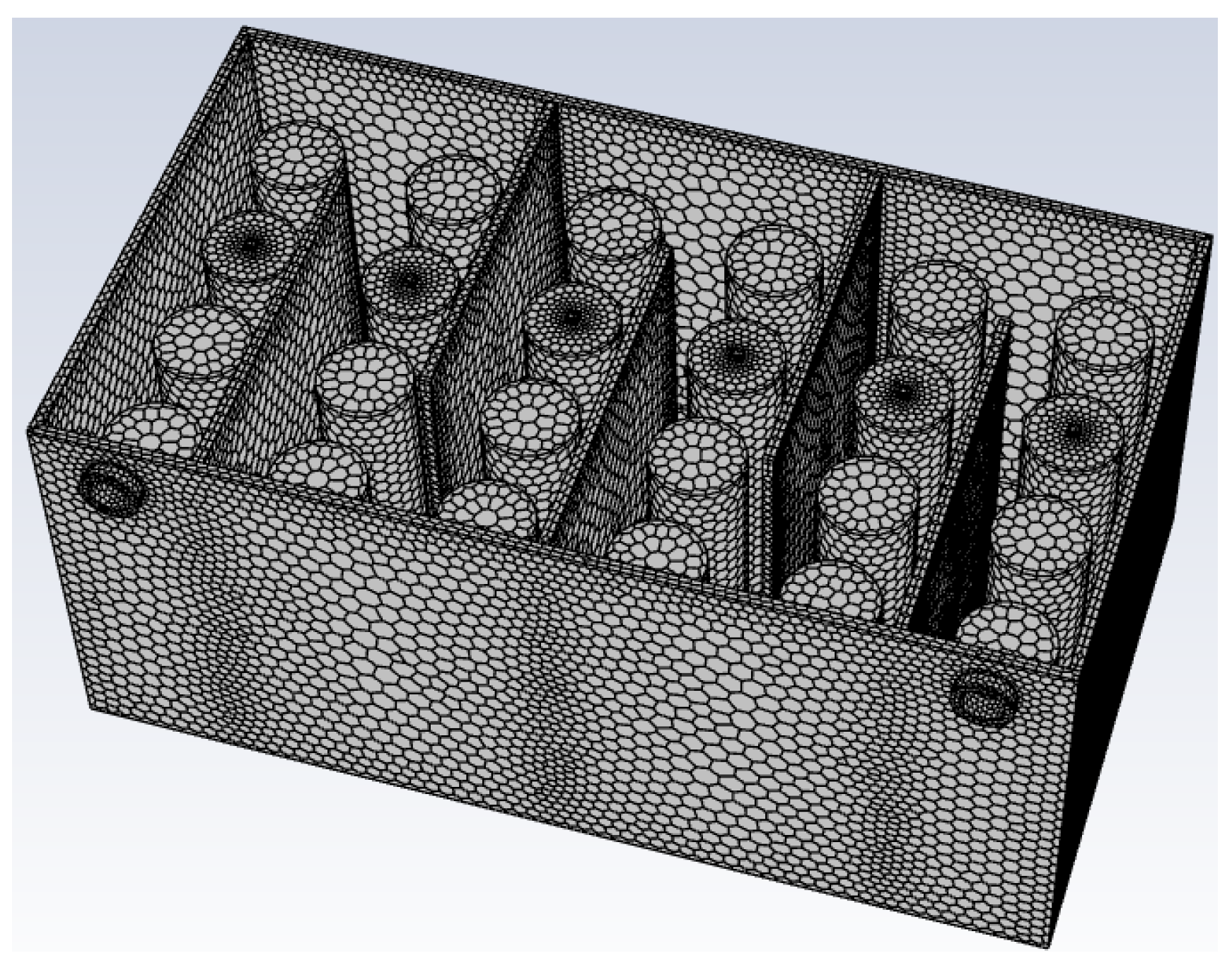
Figure 3.
Numerical result verification with experimentation: (a) Temperature tested in each channel; (b) Tave for various volume flow rates on discharge 1C, 1.5C, and 2C.
Figure 3.
Numerical result verification with experimentation: (a) Temperature tested in each channel; (b) Tave for various volume flow rates on discharge 1C, 1.5C, and 2C.
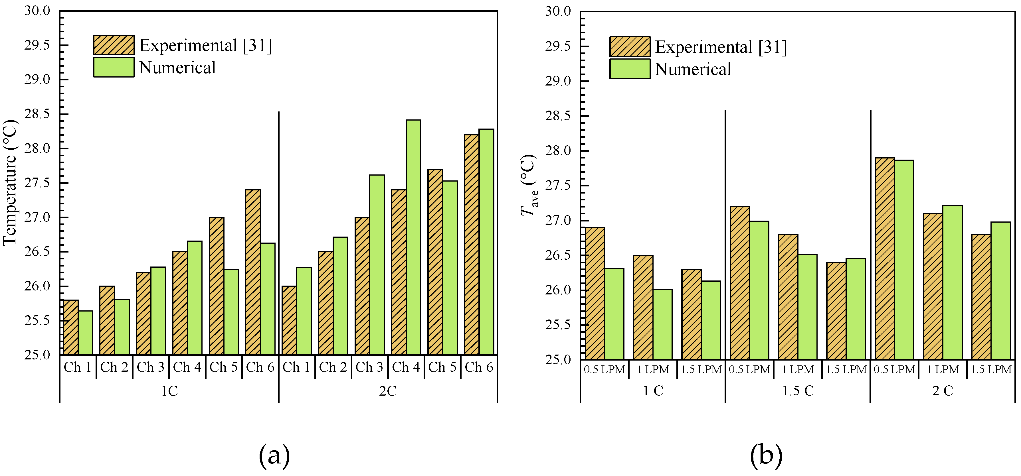
Figure 4.
Comparison of simulation values and fitting values: (a) Comparison of Tmax; (b) Comparison of Pw.
Figure 4.
Comparison of simulation values and fitting values: (a) Comparison of Tmax; (b) Comparison of Pw.
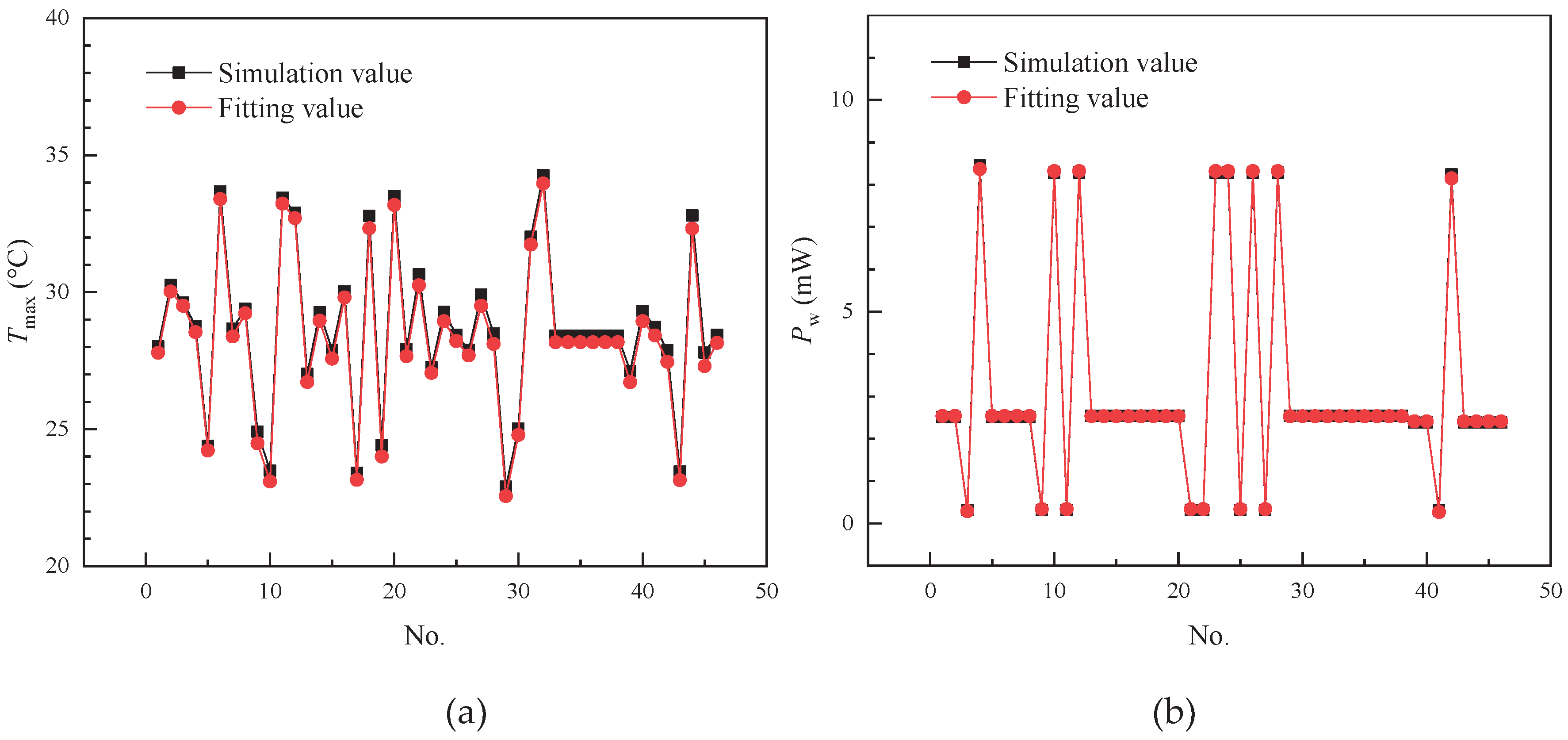
Figure 5.
RSM analysis of the combined effects for Tmax and Pw: (a) Contour of V and Crate interaction influence on Tmax (Lp =80 mm, Tin=25 °C, Tamb=30 °C); (b) Contour of V and Tin interaction influence on Tmax (Lp =80 mm, Crate =1.5 C, Tamb=30 °C); (c) Contour of V and Tamb interaction influence on Tmax (Lp =80 mm, Crate =1.5 C, Tin=25 °C); (d) Contour of V and Lp interaction influence on Pw (Crate =1.5 C, Tin=25 °C, Tamb=30 °C).
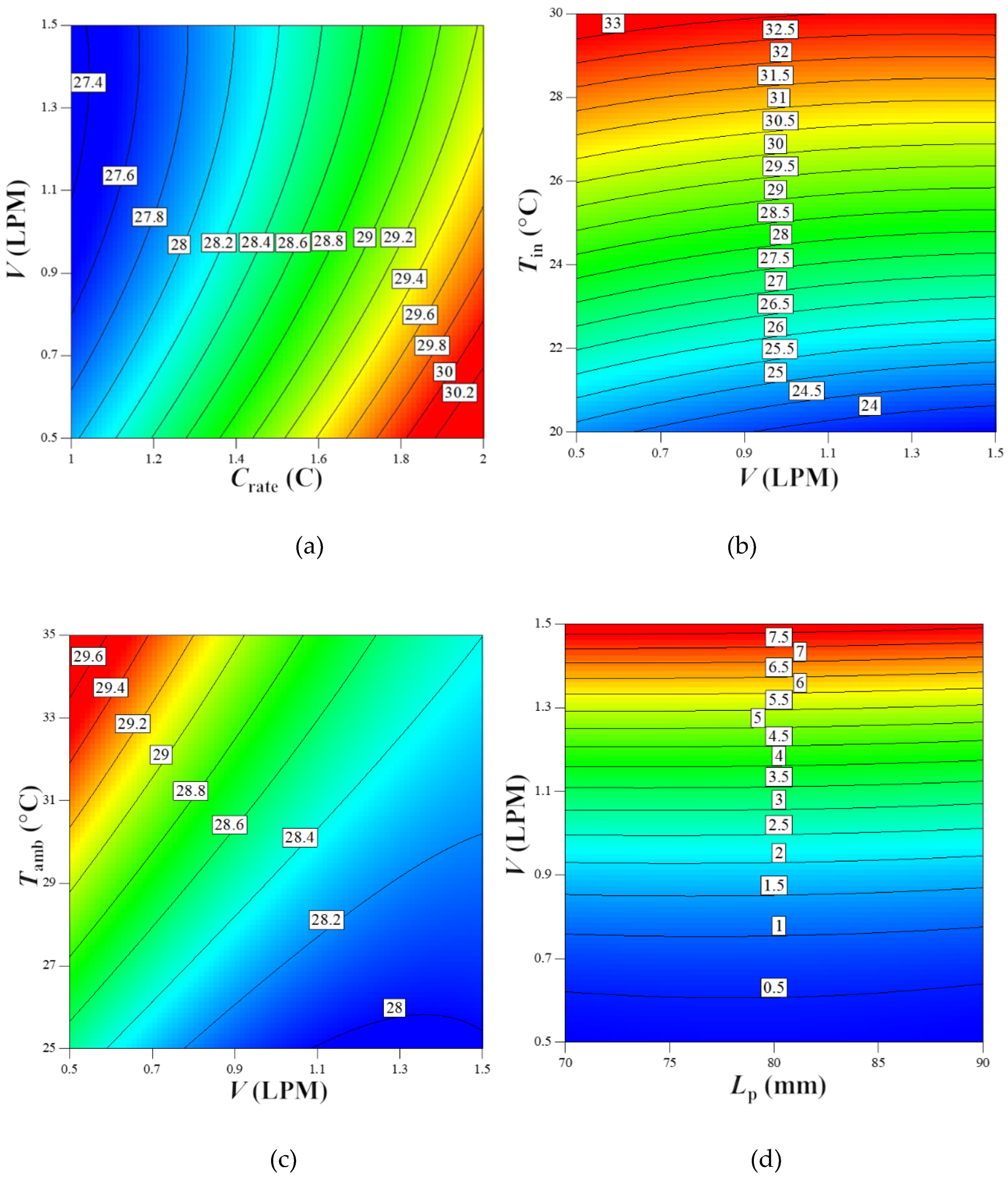
Table 3.
Grid independence check data for the numerical simulation.
| Grid density | Total elements | Tmax (°C) | Deviation of Tmax | Tave (°C) | Deviation of Tave | PW (mW) | Deviation of Pw |
| Coarse | 159350 | 27.43 | 4.33% | 25.82 | 4.51% | 2.37 | 5.58% |
| Medium | 231571 | 28.67 | 0.86% | 27.04 | 0.92% | 2.51 | 1.57% |
| Fine | 456852 | 28.92 | / | 27.29 | / | 2.55 | / |
Table 4.
Design matrix for the BBD.
| Factors | level | Units | ||
| -1 | 0 | 1 | ||
| Partitions length (Lp) | 70 | 80 | 90 | mm |
| C-rate (Crate) | 1 | 1.5 | 2 | C |
| Volumetric flow rate (V) | 0.5 | 1 | 1.5 | L/min |
| Coolant inlet temperature (Tin) | 20 | 25 | 30 | ℃ |
| Ambient temperature (Tamb) | 25 | 30 | 35 | ℃ |
Table 5.
DOE and corresponding results.
| No. | Factors | Response values | ||||||
| Lp(mm) | Crate(C) | V(L/min) | Tin(℃) | Tamb(℃) | Tmax(℃) | Tave(℃) | Pw(mW) | |
| 1 | 90 | 1.5 | 1 | 25 | 25 | 27.80 | 26.17 | 2.38 |
| 2 | 80 | 1.5 | 1.5 | 25 | 25 | 27.89 | 26.26 | 8.28 |
| 3 | 70 | 1.5 | 1 | 25 | 25 | 28.67 | 27.04 | 2.51 |
| 4 | 80 | 1.5 | 0.5 | 30 | 30 | 33.45 | 31.82 | 0.32 |
| 5 | 80 | 1.5 | 1.5 | 20 | 30 | 23.49 | 21.84 | 8.28 |
| 6 | 80 | 1.5 | 1 | 20 | 35 | 24.41 | 22.78 | 2.54 |
| 7 | 80 | 1.5 | 1 | 30 | 25 | 32.79 | 31.16 | 2.54 |
| 8 | 80 | 2 | 1.5 | 25 | 30 | 29.28 | 27.13 | 8.28 |
| 9 | 70 | 1.5 | 1.5 | 25 | 30 | 28.77 | 27.14 | 8.45 |
| 10 | 90 | 2 | 1 | 25 | 30 | 29.31 | 27.16 | 2.38 |
| 11 | 80 | 1.5 | 1 | 20 | 25 | 23.41 | 21.76 | 2.54 |
| 12 | 90 | 1.5 | 1 | 30 | 30 | 32.80 | 31.17 | 2.38 |
| 13 | 90 | 1.5 | 1 | 25 | 35 | 28.45 | 26.82 | 2.38 |
| 14 | 90 | 1.5 | 1.5 | 25 | 30 | 27.87 | 26.24 | 8.24 |
| 15 | 80 | 1.5 | 1 | 30 | 35 | 33.51 | 31.88 | 2.54 |
| 16 | 70 | 1.5 | 0.5 | 25 | 30 | 29.62 | 27.99 | 0.32 |
| 17 | 80 | 1 | 1 | 25 | 35 | 27.90 | 26.79 | 2.54 |
| 18 | 70 | 1.5 | 1 | 25 | 35 | 29.40 | 27.77 | 2.51 |
| 19 | 80 | 2 | 1 | 25 | 35 | 30.02 | 27.87 | 2.54 |
| 20 | 80 | 1.5 | 1 | 25 | 30 | 28.41 | 26.78 | 2.54 |
| 21 | 80 | 1 | 1.5 | 25 | 30 | 27.26 | 26.15 | 8.28 |
| 22 | 70 | 1.5 | 1 | 20 | 30 | 24.40 | 22.77 | 2.51 |
| 23 | 80 | 1.5 | 1 | 25 | 30 | 28.41 | 26.78 | 2.54 |
| 24 | 70 | 2 | 1 | 25 | 30 | 30.26 | 28.11 | 2.51 |
| 25 | 80 | 2 | 1 | 30 | 30 | 34.27 | 32.12 | 2.54 |
| 26 | 80 | 1.5 | 1 | 25 | 30 | 28.41 | 26.78 | 2.54 |
| 27 | 80 | 1 | 1 | 30 | 30 | 32.02 | 30.91 | 2.54 |
| 28 | 80 | 1 | 1 | 25 | 25 | 27.02 | 25.91 | 2.54 |
| 29 | 80 | 1.5 | 1 | 25 | 30 | 28.41 | 26.78 | 2.54 |
| 30 | 80 | 1.5 | 0.5 | 25 | 35 | 29.91 | 28.28 | 0.32 |
| 31 | 80 | 1.5 | 1.5 | 25 | 35 | 28.49 | 26.86 | 8.28 |
| 32 | 80 | 1.5 | 0.5 | 20 | 30 | 24.91 | 23.28 | 0.32 |
| 33 | 80 | 1.5 | 1 | 25 | 30 | 28.41 | 26.78 | 2.54 |
| 34 | 70 | 1.5 | 1 | 30 | 30 | 33.67 | 32.05 | 2.51 |
| 35 | 90 | 1 | 1 | 25 | 30 | 27.12 | 26.01 | 2.38 |
| 36 | 90 | 1.5 | 0.5 | 25 | 30 | 28.73 | 27.10 | 0.31 |
| 37 | 70 | 1 | 1 | 25 | 30 | 28.02 | 26.91 | 2.51 |
| 38 | 80 | 1.5 | 1.5 | 30 | 30 | 32.89 | 31.26 | 8.28 |
| 39 | 80 | 2 | 1 | 25 | 25 | 29.27 | 27.12 | 2.54 |
| 40 | 80 | 1.5 | 1 | 25 | 30 | 28.41 | 26.78 | 2.54 |
| 41 | 90 | 1.5 | 1 | 20 | 30 | 23.45 | 21.84 | 2.38 |
| 42 | 80 | 2 | 1 | 20 | 30 | 25.02 | 22.87 | 2.54 |
| 43 | 80 | 2 | 0.5 | 25 | 30 | 30.65 | 28.50 | 0.32 |
| 44 | 80 | 1 | 0.5 | 25 | 30 | 27.93 | 26.82 | 0.32 |
| 45 | 80 | 1.5 | 0.5 | 25 | 25 | 28.45 | 26.82 | 0.32 |
| 46 | 80 | 1 | 1 | 20 | 30 | 22.90 | 21.79 | 2.54 |
Table 6.
ANOVA for Tmax after backward elimination.
| Source | Sum of Squares | Degrees of freedom | Mean Square | F-value | p-value |
| Model | 367.77 | 11 | 33.43 | 4768.12 | < 0.0001 |
| Lp | 3.31 | 1 | 3.31 | 472.39 | < 0.0001 |
| Crate | 20.05 | 1 | 20.05 | 2859.1 | < 0.0001 |
| V | 3.72 | 1 | 3.72 | 529.84 | < 0.0001 |
| Tin | 336.81 | 1 | 336.81 | 48033.91 | < 0.0001 |
| Tamb | 2.88 | 1 | 2.88 | 410.94 | < 0.0001 |
| Crate·V | 0.1225 | 1 | 0.1225 | 17.47 | 0.0002 |
| V·Tin | 0.1849 | 1 | 0.1849 | 26.37 | < 0.0001 |
| V·Tamb | 0.1849 | 1 | 0.1849 | 26.37 | < 0.0001 |
| Lp·Lp | 0.1107 | 1 | 0.1107 | 15.79 | 0.0003 |
| Crate·Crate | 0.0956 | 1 | 0.0956 | 13.63 | 0.0008 |
| V·V | 0.4358 | 1 | 0.4358 | 62.15 | < 0.0001 |
| Residual | 0.2384 | 34 | 0.007 | / | / |
| Lack of Fit | 0.2384 | 29 | 0.0082 | / | / |
| Pure Error | 0 | 5 | 0 | / | / |
| Cor Total | 368.01 | 45 | / | / | / |
| S=0.0837 | R2=99.94% | Adjusted R2= 99.91% | Predicted R2= 99.85% | ||
Table 7.
ANOVA for Tave after backward elimination.
| Source | Sum of Squares | Degrees of freedom | Mean Square | F-value | p-value |
| Model | 353.79 | 11 | 32.16 | 4652.34 | < 0.0001 |
| Lp | 3.3 | 1 | 3.3 | 477.83 | < 0.0001 |
| Crate | 5.75 | 1 | 5.75 | 831.46 | < 0.0001 |
| V | 3.73 | 1 | 3.73 | 540.21 | < 0.0001 |
| Tin | 337.09 | 1 | 337.09 | 48760.41 | < 0.0001 |
| Tamb | 2.9 | 1 | 2.9 | 419.27 | < 0.0001 |
| Crate·V | 0.1225 | 1 | 0.1225 | 17.72 | 0.0002 |
| V·Tin | 0.1936 | 1 | 0.1936 | 28 | < 0.0001 |
| V·Tamb | 0.1849 | 1 | 0.1849 | 26.75 | < 0.0001 |
| Lp·Lp | 0.1174 | 1 | 0.1174 | 16.98 | 0.0002 |
| Crate·Crate | 0.0968 | 1 | 0.0968 | 14.01 | 0.0007 |
| V·V | 0.4316 | 1 | 0.4316 | 62.43 | < 0.0001 |
| Residual | 0.235 | 34 | 0.0069 | / | / |
| Lack of Fit | 0.235 | 29 | 0.0081 | / | / |
| Pure Error | 0 | 5 | 0 | / | / |
| Cor Total | 354.02 | 45 | / | / | / |
| S=0.0831 | R2=99.93% | Adjusted R2= 99.91% | Predicted R2= 99.85% | ||
Table 8.
ANOVA for Pw after backward elimination.
| Source | Sum of Squares | Degrees of freedom | Mean Square | F-value | p-value |
| Model | 288.68 | 5 | 57.74 | 62311.83 | < 0.0001 |
| Lp | 0.0625 | 1 | 0.0625 | 67.45 | < 0.0001 |
| V | 254.56 | 1 | 254.56 | 2.75E5 | < 0.0001 |
| Lp·V | 0.01 | 1 | 0.01 | 10.79 | 0.0021 |
| Lp·Lp | 0.0346 | 1 | 0.0346 | 37.33 | < 0.0001 |
| V·V | 32.93 | 1 | 32.93 | 35538.51 | < 0.0001 |
| Residual | 0.0371 | 40 | 0.0009 | / | / |
| Lack of Fit | 0.0371 | 35 | 0.0011 | / | / |
| Pure Error | 0 | 5 | 0 | / | / |
| Cor Total | 288.72 | 45 | / | / | / |
| S=0.0304 | R2=99.99% | Adjusted R2= 99.99% | Predicted R2= 99.97% | ||
Table 9.
Regression coefficient.
| Regression coefficient | Response | ||
| Tmax (°C) | Tave (°C) | Pw (W) | |
| a0 | 11.240 | 11.404 | -2.292 |
| a1 | -0.214 | -0.220 | 0.097 |
| a2 | 1.758 | 0.711 | / |
| a3 | -1.164 | -1.208 | -5.597 |
| a4 | 0.832 | 0.830 | / |
| a5 | 0.171 | 0.171 | / |
| a6 | / | / | -0.010 |
| a7 | -0.700 | -0.700 | / |
| a8 | 0.086 | 0.088 | / |
| a9 | -0.086 | -0.086 | / |
| a10 | 0.001 | 0.001 | -5.82e-4 |
| a11 | 0.393 | 0.396 | / |
| a12 | 0.840 | 0.836 | 7.187 |
Table 10.
The optimal point for Tmax, Tave and Pw.
| Lp (mm) | Crate(C) | V(LPM) | Tin(℃) | Tamb(℃) | Tmax(℃) | Tave(℃) | Pw(mW) | Composite desirability |
| 89.5 | 1.08 | 0.51 | 20 | 25.62 | 22.87 | 21.67 | 0.279 | 1 |
Disclaimer/Publisher’s Note: The statements, opinions and data contained in all publications are solely those of the individual author(s) and contributor(s) and not of MDPI and/or the editor(s). MDPI and/or the editor(s) disclaim responsibility for any injury to people or property resulting from any ideas, methods, instructions or products referred to in the content. |
© 2025 by the authors. Licensee MDPI, Basel, Switzerland. This article is an open access article distributed under the terms and conditions of the Creative Commons Attribution (CC BY) license (http://creativecommons.org/licenses/by/4.0/).
Copyright: This open access article is published under a Creative Commons CC BY 4.0 license, which permit the free download, distribution, and reuse, provided that the author and preprint are cited in any reuse.


