
Submitted:
25 June 2025
Posted:
26 June 2025
You are already at the latest version
Abstract
Each charging/discharging cycle leads to a gradual decrease of the battery’s capacity. Degradation of capacity in lithium-ion batteries represents a non-monotonous process with random jumps. Earlier studies claimed that the instantaneous degradation value of lithium-ion battery is influenced by the historical data, demonstrating long-range dependence. The existing methods ignore large jumps and long-range dependence in degradation processes. In order to capture long-range dependent property and random jumps, we deal with the fractional Poisson process. We also outline the relationship between the long-range correlation and the Hurst index. The connection between random jumps in capacitance and long-range dependence of the fractional Poisson process is proven. In order to construct the fractional Poisson predictive model, we included the fractional Brownian motion as the diffusion term and the fractional Poisson process as the jump term. The efficiency of our approach for calculation of the random walk was tested on the NASA’s dataset of Li-ion battery dataset. We claim that the predictive model based on the fractional Poisson process has a number of advantages over the fractional Brownian motion, fractional Levy stable motion, the Wiener model and the Long-Short Term Memory model.
Keywords:
fractional Poisson process
; long-range dependence
; Hurst exponent
; remaining useful life
1. Introduction
The capacity of lithium-ion batteries (LIBs) has a degradation trend with charging and discharge cycles. This results in the reduction of the end of life (EOL). A recommended practice to replace the battery on the capacity basis is estimated below 80% of the manufacturer’s rating [IEEE 1188-1996]. Widespread applications of LIBs demand accurate prediction of RUL of LIBs.
Xiong et al. [1] deduces mathematical equations through electrochemical theory and applies finite element analysis and numerical methods to solve equations to build a predicting model. Li et al. [2] proposed to simulate the battery load response under specific temperature conditions through a coupling model, which is suitable for the temperature range of 25℃ to 40℃ in daily life. Using circuit theory to explore and analyze the performance of batteries [3], the Rint model and impedance-capacitor (RC) network model [4] are classic examples of such methods. Through a large amount of historical degradation data, based on the capacity transfer relationship of the battery at adjacent time points, and applying Kulun's law, the capacity loss of the battery is modeled, and then a polynomial and exponential decay model is derived [5]. Most empirical models rely on statistical random filtering technology to track battery decay trends and optimize model parameters, such as particle filtering, Kalman filtering, etc. [6]. The prediction accuracy is highly dependent on the of model construction. Focusing on the research of data-driven methods, Chen et al. [7] combined variable modal decomposition and GPR, first decompose the capacity degradation data of lithium batteries into relatively stable components, and then conduct RUL prediction based on these components.
Li et al. [8] proposed a GPR prediction model with an automatic selection mechanism of kernel function. Jia et al. [9] mined key features from charge and discharge data, and then used GPR to estimate SOH and RUL, and effectiveness is proved. Peikun et al. [10] combined with gray correlation analysis and GPR method of multi-island genetic algorithm to optimize the prediction of SOH accuracy. these methods need high standards for data collection.
Xiao et al. [11] proposed a prediction technology combining RVM and three-parameter capacity decay model, Feng et al. [12] explored health indicator extracted from surface temperature changes when battery discharged, and Wang et al. [13] extracted new health indicator from the current curve during constant voltage charging of the battery. The RVM model is an emerging data-driven method, but its inherent high sparsity means that direct use of RVM for prediction may lead to instability of predicting result [14].
Deep learning such as recurrent neural network (RNN) is used for battery RUL prediction. Researchers [15] extracted key features of degradation data through empirical modal decomposition and grey relationship analysis, and used these features to deep RNNs to simulate cell RUL.
The current methods can only predict the volatility of the degradation trend. The fPp process can simulate irregular jumps caused by emergencies such as overcharge, short circuit or temperature abnormalities, and capacity regeneration, and can capture the continuous trend-long correlation and random fluctuations in the data.
The above methods can only predict the undulatory property of degradation trend, without considering the long-range dependence of lithium battery degradation process and the irregular jumps caused by capacity regeneration due to overcharge, short circuit or abnormal temperature emergencies. This paper proposes that the fPp prediction model can capture the long-range dependence property and random jump.
The organization of this paper is as follows. Section 2 discuses Long-range Dependence and Poisson Distribution, Section 3 Definition and characteristic of fractional Poisson process(fPp) Section 4 constructs a stochastic differential equation with adaptive jump intensity based on the fPp process. Section 5 is parameter estimation, section 6 is case study, section 7 is conclusion.
2. Long-Range Dependence and Poisson Distribution
2.1. Long-range Dependence
An autocorrelation function of a random series is a measure of the dependence of time series under different time interval(i.e. delays). Given a random sequence , its autocorrelation function see equation (1):
Because decay is very slow, it means that is significant correlation between sequence values even after a long lag. decays obeys power law, see equation(2):
where and c are a constant, H is the Hurst exponent, and its range is, which is used to determine whether a random process has the LRD characteristic. When , the autocorrelation function can be integrated or summed, meaning that the random sequence is not autocorrelation characteristics; when , the autocorrelation function cannot be integrated or summed, revealing that the random sequence exhibits correlation, where shows a short correlation, and when , the random process exhibits LRD characteristics.
2.2. Estimation of the Hurst exponent
A number of estimation algorithms of the Hurst exponent were proposed. Here, the heavy scale extreme difference method is used, namely the R/S method, which is as follow:
Divide the random sequence into subsequence of length . The average value of these subsequenece is as follows (3):
Calculate the cumulative deviation, as shown in Equation (4):
Calculate the extreme difference value, as shown in Equation (5)
Calculate the standard deviation, as shown in Equation (6)
Calculate the standard deviation, as shown in Equation (7)
Next, repeat the above steps, and on the premise that the formula (6) is satisfied, take different , get . Finally, the re-scaling extreme difference takes the logarithm and fits the straight line using the least squares method, as shown in equation (8):
The slope ratio is the desired H, see Figure 1.
2.3. Jump Characteristics of Poisson Distribution
For any time length , the probability of occurring n events obeys the Poisson distribution, as follows (9)
Where is the average times number occurs in unit time, and is recorded as .
2.4. Random walks characteristics of Poisson distribution
A Poisson process , defines , as a random walk approximation of is described as in Equation (10):
Where is a random variable with independent and homogeneous distribution. For , there is the probability of formula (11):
where . Let , is the Poisson random walk process, see Figure 3. When increases, the irregularity is stronger.
3. Definition and Characteristics of the Fractional Poisson Process
According to Wang et al. [16], the fPp is defined as a class of non-Gaussian processes with stationary increments, and the definition of is given as follows (12):
where .
According to equation (12), when , represents short-term correlation, when is a typical Poisson process. when , fPp has LRD properties. Obviously, the Poisson process is actually only a special case of fPp. The curve of the Hurst exponent with time is shown in Figure 4, and the Hurst ranges is from 0.5 to 0.1. The higher the surface curve, the stronger the long-range dependence.
4. Fractional Poisson process predictive model
For any random sequences , using the Black–Scholes formula, we can obtain a random differential equation based on Brownian motion, such as equation (13):
where and are the drift and diffusion coefficients, respectively; is the Brownian motion, and is replaced by fBm, thus the equation (13) has LRD characteristics, shown as equation (14), which can more accurately simulate the remaining useful life decay process of lithium batteries.
Where is the fBm process, is the fPp process, is the jump amplitude, and discretization can obtain the discrete equation (15).
the fPp difference prediction degradation model is deduced, as shown equation (16):
let ,,,,,,,substituing into equation (16),get random sequence simulation, as shown Figure 5.
5. Parameter estimation
5.1. Estimation of drift and diffusion coefficients
For model (16), the maximum likelihood method is applied to estimate the parameters. let sample , the joint probability density is as follows:
Two side takes logarithm(18)
Take the partial derivative for parameter and , and let them equal zero, respectively, get equation (19) , (20) and(21)
5.2. Estimation Parameter
First calculate the difference for , shown as equation (22)
Where is the battery capacity of the ith times charge or discharage period, here let 95th percentile as jump threshold, shown as equation (23)
Record jump times:
When given a Poisson process, the probability of occur times events during follows:
Construct the logarithmic likelihood function
By using the properties of logarithm equation (26) can be expanded as follows:
Then we obtain:
where represents the exponent function for , is equal to 1, otherwise it is equal to zero.
6. Case Study
This experiment used the RW12 degradation walk data set of four 18650 lithium batteries from NASA[17], which operated continuously at charge and discharge currents between -4.5A and 4.5A. This type of charging and discharging operation is called random walking (RW) operation. Each load period lasts for 5 minutes, and after 1500 cycles (approximately 5 days), a series of reference charge and discharge cycles are performed to provide a reference standard for the health of the battery. The voltage, current and temperature changes of lithium battery during the charge and discharge cycle are shown in Figure 6:
The capacity of RW12 battery is degraded as shown in Figure 7. The battery fails when the capacity EOL is set to 1.4Ah in this article. Therefore, the RW12 battery fails after the 56th cycle.
By degrading the data difference of RW12, the jump situation as shown in Figure 8(a) is obtained. Four points exceed the 95% threshold, so there is a situation that the fBm model cannot predict. As shown in Figure 8(b), the large jump point has both capacity regeneration and significant decline in capacity, which is suitable for RUL prediction using the fPp degradation model.
The result of our simulation is shown in Figure 9 (a); the gray area in Figure 9 (b) represents that the different values are within the error of 10%, i.e., the predicted values have an acceptable error.
The error analysis of the fPp RUL prediction for battery RW12 is shown in Table 1.
Comparing with the fBm model, LSTM model, fLsm model and Wiener model, Through the error analysis of MAE, MAPE, RMSE and , the prediction error evaluation of the fPp model is the smallest,see Table 2.
Table 2 are visualized as a histogram, see Figure 10. From Figure 10 (a), (b), and (c), it is evident that the fPp model has the lowest prediction error. Furthermore, Figure 10 (d) clearly shows that the fPp model's prediction result is close to 1, it is mean that the fPp degradation model has high accuracy.
6. Conclusion
By the NASA degradation walk data set, the effectiveness of the fPp differential degradation model with the capacity regeneration jumps was verified, and parameter can describe jumps. The walk degradation data satisfies the LRD and determines the EOL. By selecting different prediction starting points, the results of parameter estimation are fed into the fPp degradation model to obtain the PDF and RUL predictions. Finally, the fBm model, LSTM model, fLsm model, and Wiener model were used as comparison models to verify the effectiveness of the fPp degradation model.
Author Contributions
Conceptualization, Song W.Q.; methodology, Jing Shi; software, Jing Shi, and Feng L; validation, Aleksey K. and Wu Z.Y.; formal analysis, Aleksey K..; investigation,Wu Z.Y.; resources,Aleksey K. and Song W.Q.; data curation, Song W.Q; writing—original draft preparation, Jing Shi;; writing—review and editing, Aleksey K. ; visualization, Wu Z.Y; supervision, Song W.Q;.; project administration, Song W.Q..; funding acquisition, Jing Shi.
Acknowledgments
This research was supported by Science and Technology Plan Fund Project of the Fujian Provincial Department of Science and Technology, China(No. 2024H0038), and Scientific Research and Innovation Team of Minnan University of Science and Technology (No.2024XTD160).
Conflicts of Interest
The authors declare no conflicts of interest.
Abbreviations
| RUL | Remaining useful life |
| LRD | Long-range dependence |
| fPp | Fractional Poisson process |
| fBm | Fractional Brownian motion |
| fLsm | fractional Lévy stable motion |
| EOL | End of life |
| Probability density motion | |
| LSTM | Long-short term memory |
| GPR | Gaussian process regression |
| RVM | Relevance vector machine |
| RNN | Recurrent neural network |
| SOH | State of Health |
| Fractional Poisson process | |
| Fractional Brownian motion | |
| Hurst exponent | |
| The intensity of jumping | |
| Drift coefficient | |
| Diffusion parameter |
References
- Zhi Y, Wang H, Wang L. A state of health estimation method for electric vehicle Li-ion batteries using GA-PSO-SVR, Complex & Intelligent Systems, 2022, 8(3): 2167-2182. [CrossRef]
- Cho K, Kim S, Kim S, et al. Electrochemical Model-Based State-Space Approach for Real-Time Parameter Estimation of Lithium-Ion Batteries, Electro chemical Society Meeting Abstracts 244. The Electro chemical Society, Inc., 2023 (65):3052 -3052.
- Wang Y, Tian J, Sun Z, et al. A comprehensive review of battery modeling and state estimation approaches for advanced battery management systems, Renewable and Sustainable Energy Reviews, 2020, 131: 110015. [CrossRef]
- Liu W, Placke T, Chau K T. Overview of batteries and battery management for electric vehicles, Energy Reports, 2022, 8: 4058-4084. [CrossRef]
- Sui X, He S, Vilsen S B, et al. A review of non-probabilistic machine learning-based state of health estimation techniques for Lithium-ion battery, Applied Energy, 2021, 300: 117346. [CrossRef]
- Severson K A, Attia P M, Jin N, et al. Data-driven prediction of battery cycle life before capacity degradation, Nature Energy, 2019, 4(5): 383-391. [CrossRef]
- Chen J C , Chen T L , Liu W J ,et al.Combining empirical mode decomposition and deep recurrent neural networks for predictive maintenance of lithium-ion battery, Advanced Engineering Informatics, 2021, 50:101405.
- Li X, Yuan C, Wang Z. Multi-time-scale framework for prognostic health condition of lithium battery using modified Gaussian process regression and nonlinear regression,Journal of Power Sources, 2020, 467: 228358.
- Jia J , Liang J , Shi Y ,et al.SOH and RUL Prediction of Lithium-Ion Batteries Based on Gaussian Process Regression with Indirect Health Indicators, Energies, 2020, 13(2):375.
- Peikun S , Zhenpo W .Research of the Relationship between Li-ion Battery Charge Performance and SOH based on MIGA-Gpr Method, Energy Procedia, 2016, 88:608-613. [CrossRef]
- Xiao Y, Deng S, Han F, et al. A Model-Data-Fusion Pole Piece Thickness Prediction Method With Multisensor Fusion for Lithium Battery Rolling Machine, IEEE Access, 2022, 10: 55034-55050. [CrossRef]
- Feng H , Song D .A health indicator extraction based on surface temperature for lithium-ion batteries remaining useful life prediction,The Journal of Energy Storage, 2021, 34:102118. [CrossRef]
- Wang R, Feng H. Remaining useful life prediction of lithium-ion battery using a novel health indicator, Quality and Reliability Engineering International, 2021, 37(3): 1232-1243. [CrossRef]
- Hu C, Youn B D, Wang P, et al. Ensemble of data-driven prognostic algorithms for robust prediction of remaining useful life, Reliability Engineering & System Safety, 2012, 103: 120-135. [CrossRef]
- Chen J C , Chen T L , Liu W J ,et al.Combining empirical mode decomposition and deep recurrent neural networks for predictive maintenance of lithium-ion battery. Advanced Engineering Informatics, 2021, 50:101405.
- Wang X T, Wen Z X, Zhang S Y. Fractional poisson process (ii), Chaos, Solitons & Fractals, 2006, 28(1): 143-147.
- Saha B, Goebel K. Battery data set, NASA AMES prognostics data repository, 2007.
Figure 1.
Estimation of the Hurst exponent.
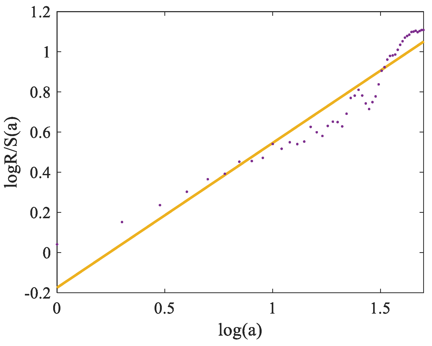
Figure 2.
Poisson Process Describing Sudden Events.
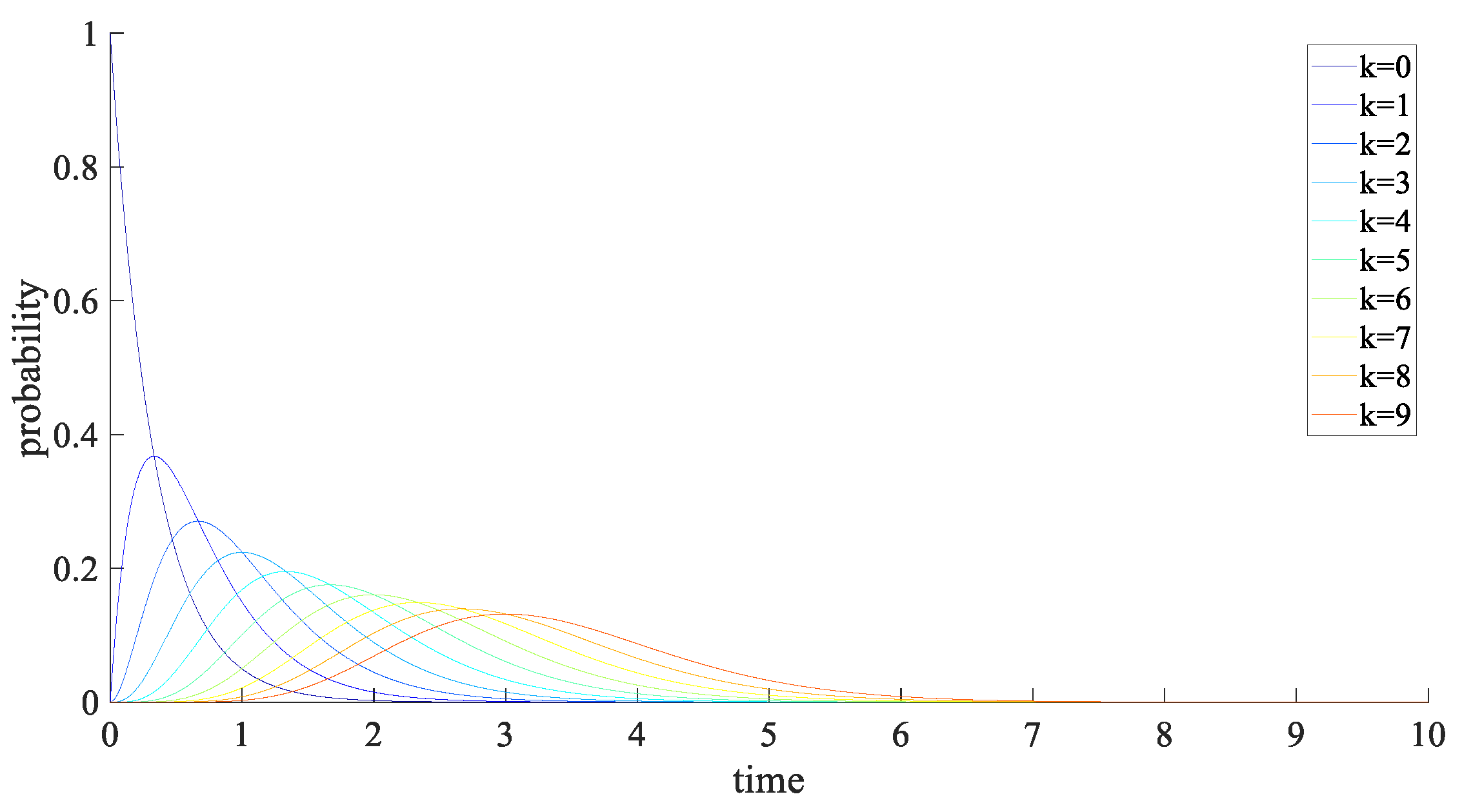
Figure 3.
Random walk approximation.
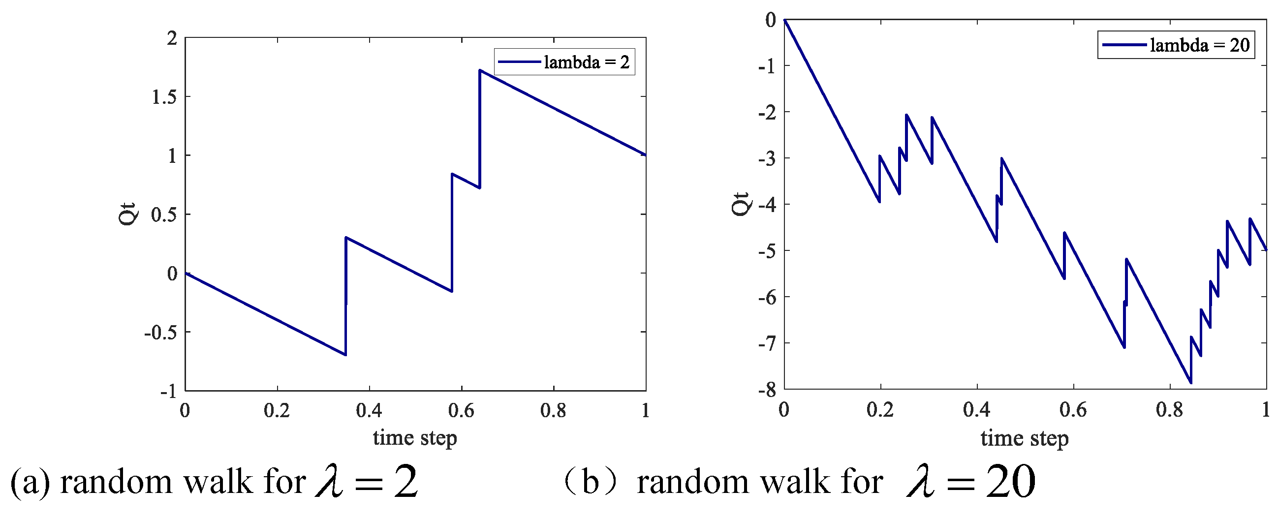
Figure 4.
Autocorrelation Function of fPp with Different Hurst Exponents.
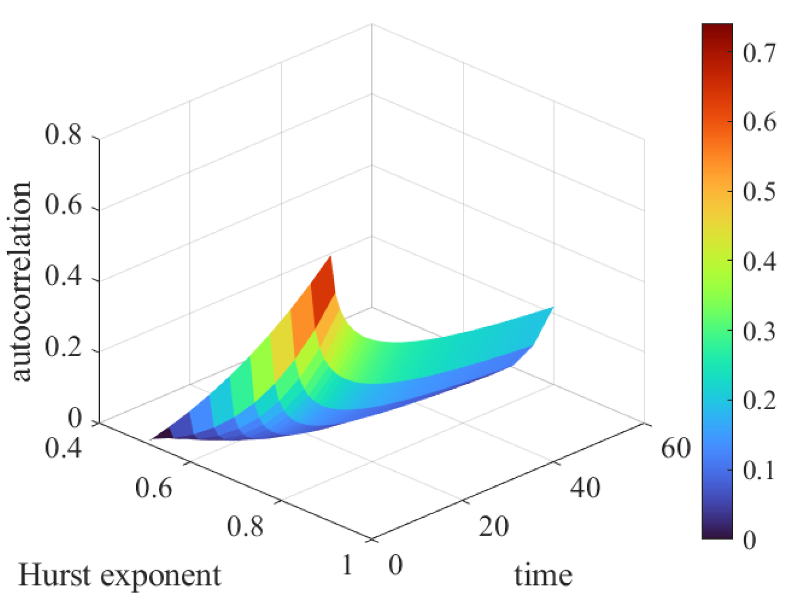
Figure 5.
Differential equation numerical simulation.
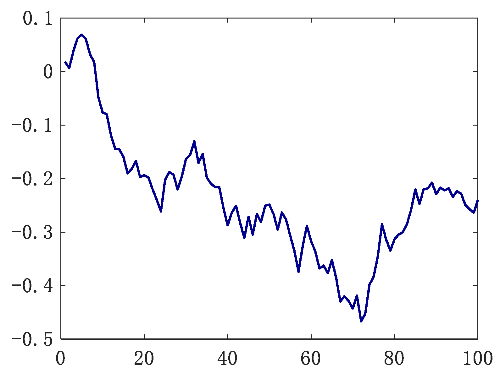
Figure 6.
Voltage, Current, and Temperature during the cycles charge-discharge.
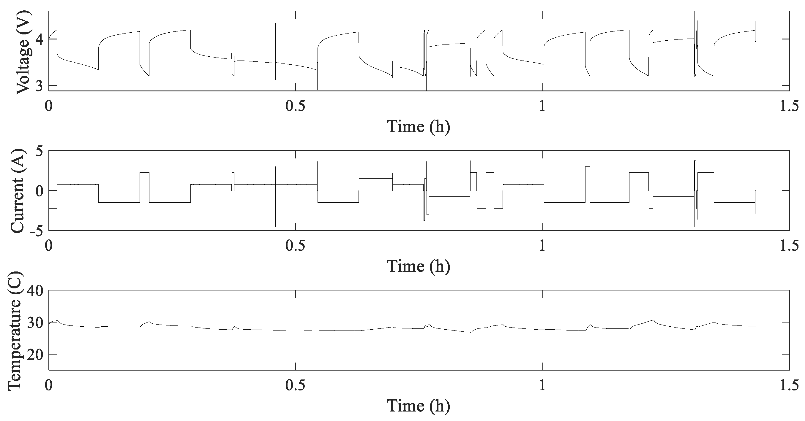
Figure 7.
Capacity Degradation and the Failure Threshold.
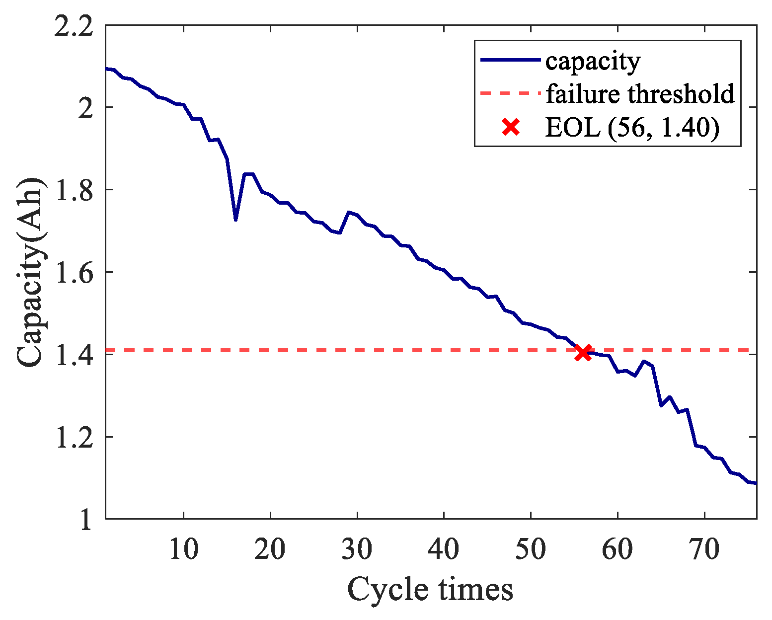
Figure 8.
Capacity Differential and Large Jump of RW12.
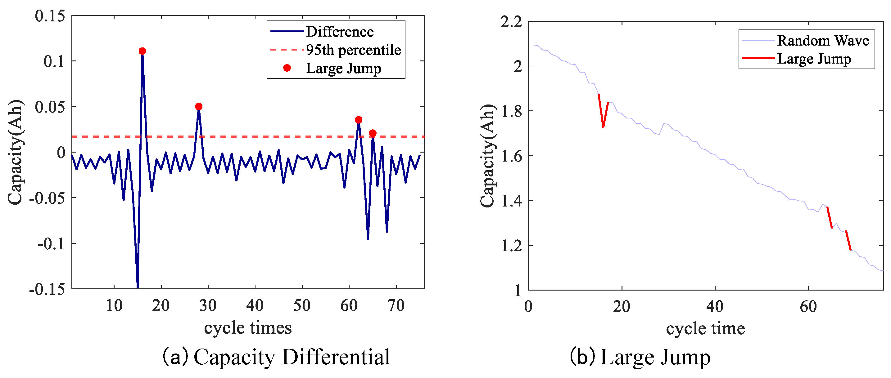
Figure 9.
RUL prediction results and performance Region of RW12.
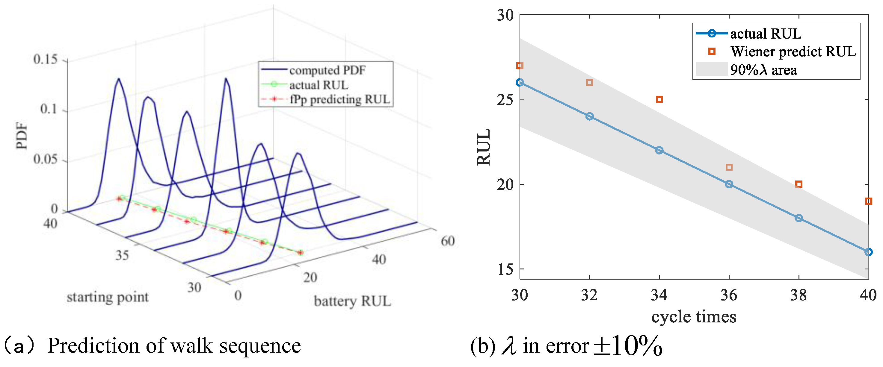
Figure 10.
Performance Evaluation of three Models.
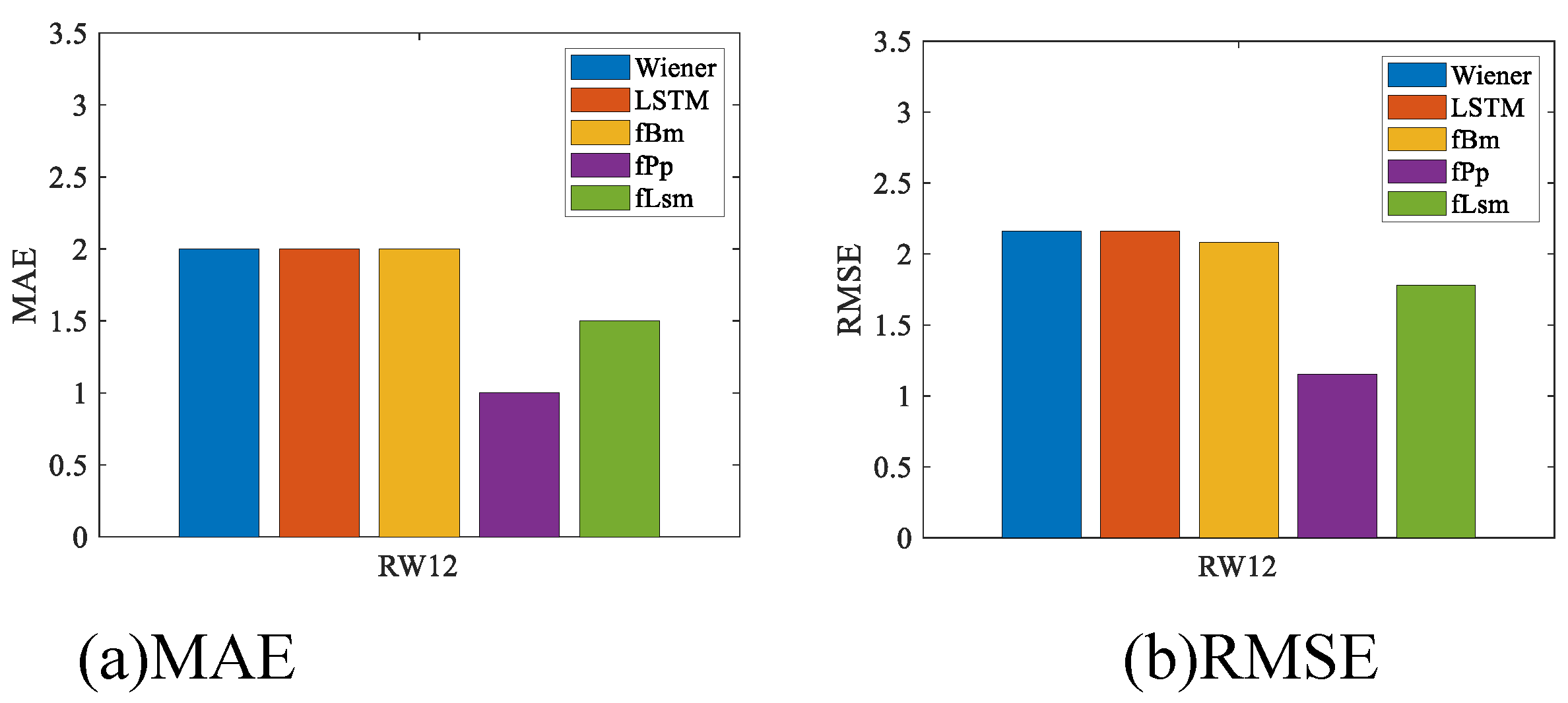
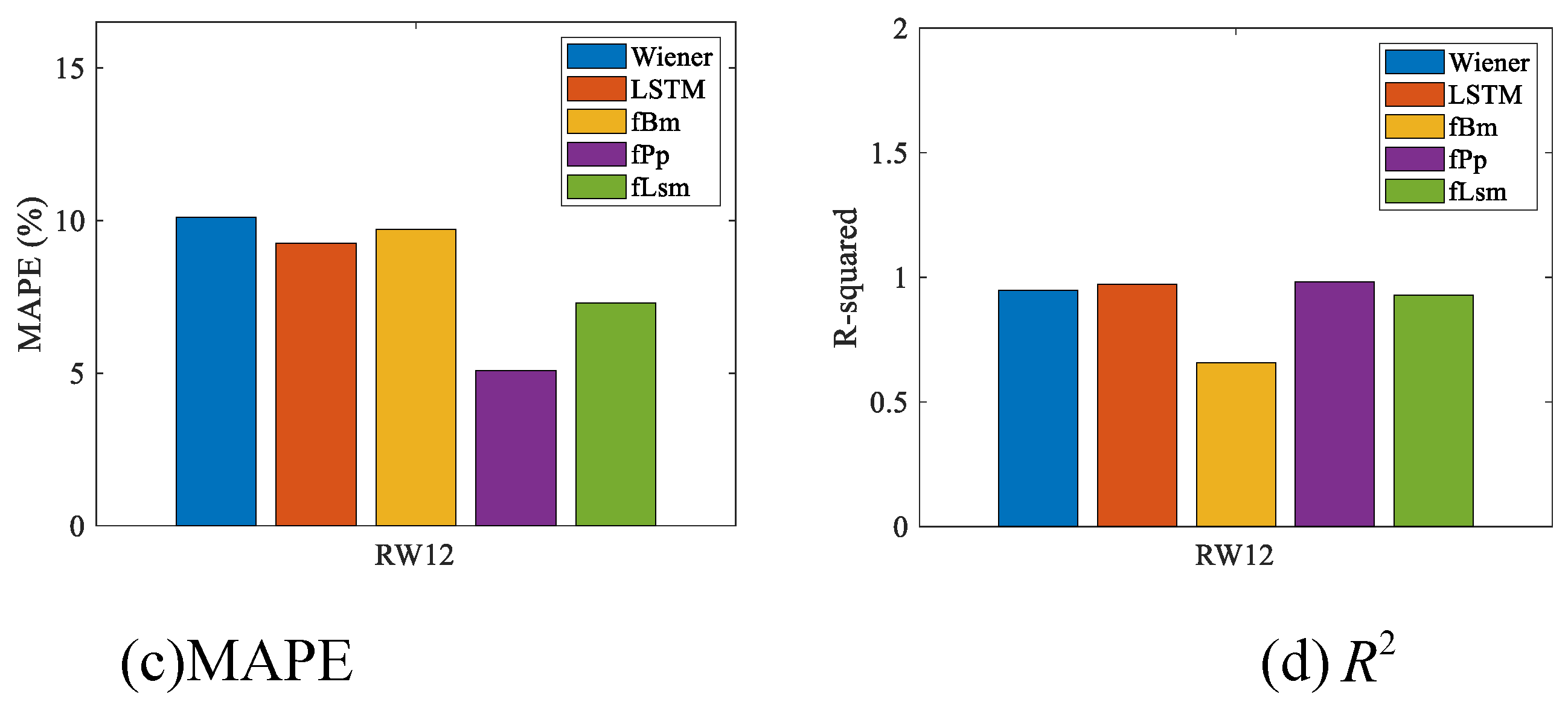

Table 1.
fPp model prediction results and error analysis of RW12.
| Start point | RUL actual | RULpredict value | AE | RE |
| 30 | 26 | 26 | 0 | 0.0000 |
| 32 | 24 | 23 | 1 | 0.0417 |
| 34 | 22 | 21 | 1 | 0.0455 |
| 36 | 20 | 18 | 2 | 0.1000 |
| 38 | 18 | 17 | 1 | 0.0556 |
| 40 | 16 | 15 | 1 | 0.0625 |
Table 2.
Comparative Prediction Evaluation of fPp Model and Benchmark Models.
| battery | Model | MAE | MAPE(%) | RMSE | |
| RW12 | fPp | 1.0000 | 5.0863 | 1.1547 | 0.9823 |
| fBm | 2.0000 | 9.7122 | 2.0817 | 0.6577 | |
| LSTM | 2.0000 | 9.2484 | 2.1602 | 0.9725 | |
| fLsm | 1.5000 | 7.2959 | 1.7795 | 0.9292 | |
| Wiener | 2.0000 | 10.1128 | 2.1602 | 0.9468 |
Disclaimer/Publisher’s Note: The statements, opinions and data contained in all publications are solely those of the individual author(s) and contributor(s) and not of MDPI and/or the editor(s). MDPI and/or the editor(s) disclaim responsibility for any injury to people or property resulting from any ideas, methods, instructions or products referred to in the content. |
© 2025 by the authors. Licensee MDPI, Basel, Switzerland. This article is an open access article distributed under the terms and conditions of the Creative Commons Attribution (CC BY) license (http://creativecommons.org/licenses/by/4.0/).
Copyright: This open access article is published under a Creative Commons CC BY 4.0 license, which permit the free download, distribution, and reuse, provided that the author and preprint are cited in any reuse.


