
Submitted:
24 June 2025
Posted:
26 June 2025
You are already at the latest version
Abstract
PM2.5 air pollution has become a critical environmental concern in Korea, requiring accurate forecasting systems for effective air quality management and public health protection. Numerical models face limitations including high computational costs, complex processes, and parameterization uncertainties. This study developed an LSTM-based PM2.5 forecasting model for the Seoul area using integrating observational data and numerical model outputs to overcome the limitations. To address input data gaps in future time steps where observational data are unavailable, WRF-CMAQ model outputs are incorporated as supplementary inputs. Three LSTM models with different training periods are developed: T3V19(3-year), T5V21(5-year), and T6V22(6-year training). Performance evaluation during January-March 2023 demonstrated significant improvements over the CMAQ model. The T6V22 model achieves a 96% improvement in NMB (1.3 vs. 32% for CMAQ), meeting “Goal” benchmark criteria. The correlation coefficient increased from 0.79 to 0.85, while NME decrees from 43.3% to 22.6%. LSTM models consistently outperformed conventional numerical models across all forecast lead times (D+0, D+1, D+2). The results suggest that as input data volume increases, model performance becomes more superior and enables more stable air quality predictions, providing a promising framework for operational forecasting systems
Keywords:
artificial intelligence (AI)
; long short-term memory (LSTM)
; PM2.5
; air quality forecast
; big data
1. Introduction
Air pollution has now become one of the most significant environmental concerns due to its detrimental effects on human health such as disease and mortality and the environment in the world, especially in Korea (WHO, 2016). Therefore, real-time PM2.5 concentration predictions in advance have significant practical and social values, which play a significant role in making atmospheric management decisions to control air pollution and are important information needed to facilitate sustainable development.
PM2.5 forecasting methods can be classified into numerical models and statistical models. Numerical models for forecasting PM2.5 are mainly used the Community Multiscale Air Quality (CMAQ) model (Zhang et al., 2022; Chang et al., 2021; TT de Almeida et al., 2018; Tao et al., 2020), CMAS (Flemming et al., 2017), WRF-Chem models (Reyes-Villegas et al., 2023; Li et al., 2023; Ma et al., 2018; Wang et al., 2020) and GEOS-Chem models (Yang and Zhao, 2023; Kumar et al., 2021; Travis et al., 2022). However, due to the complex pollutant diffusion mechanism, some problems produced by these models result in usage limitations, such as colossal calculation workload, the complexity of the process, uncertainty of parameters (Gao and Zhou, 2024, Huang et al., 2021; Ferreira et al., 2020; Sokhi et al., 2021; Baklanov et al., 2020).
Statistical models for forecasting PM2.5 are based on statistics and use historical time series data to predict future PM2.5 concentration. As historical observational data of air quality continues to accumulate and the demand for more efficient and accurate forecasting grows, machine learning methods—recognized for their strong predictive capabilities—have emerged in forecasting PM2.5 in recent years research (Do et al., 2023; Karimian et al., 2019; Vignesh et al., 2023). Compared with numerical models, the statistical prediction models not only avoid the complicated mechanism so that the model forecasts PM2.5 concentration faster, and the cost of each prediction can be reduced but also can achieve an almost improved level of PM2.5 concentration prediction accuracy of the physical prediction models.
Recently, long short-term memory neural network (LSTM; Hochreiter and Schmidhuber, 1997) has been used extensively for forecasting time-series data as a type of machine learning method due to its capability of simulating long and short-term tendencies simultaneously. Qadeer et al. (2020) shows that LSTM demonstrated the outstanding accuracy compared to gradient tree boosting models, RNN, and CNN in forecasting PM2.5 concentrations. Li et al. (2017) constructed a method of using the historical concentrations of all sites as the inputs of the LSTM and integrating auxiliary variables by a fully connected layer. As prediction of PM2.5 concentration increasingly adopts deep learning (DL) approaches, it is becoming evident that the performance and applicability of DL-based models depend more critically on quality and consistency of datasets than on the choice of algorithms.
In this study, we develop a model employing LSTM algorithm to overcome the limitations of numerical models and improve the accuracy of PM2.5 forecasts. We evaluated the model’s performance with respect to datasets enhancement for PM2.5 forecasting.
2. Input Data Collection and Preprocessing
2.1. Observational Meteorological and Air Quality Data
The meteorological data used in the model is based on real-time ASOS (Automated Surface Observing System) data obtained via API system of KMA (Korea Meteorological Administration). Although ASOS instruments collect a wide range of meteorological data, this study selected six key variables that are most relevant to the formation and dispersion of PM2.5. The first variable considered is air temperature, which exhibits a distinct diurnal cycle and can influence the increase or decrease of PM2.5 (Li et al., 2022). Increasing temperatures contribute to the enhanced chemical formation and accumulation of PM2.5. Dew temperatures and relative humidity, which serve as indicators of atmospheric moisture content, have been suggested to positively influence PM2.5 concentrations, as increased atmospheric humidity provides favorable conditions for aerosol formation and hygroscopic growth (Cheng et al., 2015). Wind speed, one of the key meteorological variables influencing the formation and dispersal of PM2.5, is negatively correlated with PM2.5 concentrations (Yu et al., 2018, Eun et al., 2020). Fujino and Miyamoto (2022) suggest that the scavenging efficiency was 2.03% for light precipitation, 28.15% for moderate precipitation, and 26.75% for heavy precipitation, suggesting that moderate or stronger rainfall is more effective in removing PM2.5 concentration. This implies that wet deposition processes such as rainout and washout play a significant role in reducing PM2.5 concentration during precipitation events. Precipitation duration, along with intensity, exerts a direct influence on PM2.5 concentration and should therefore be regarded as a key meteorological variable in PM2.5. The synoptic system which influences PM2.5 can be represented by sea level pressure (SLP). Chang et al. (2020) identified high-pressure systems as dominant synoptic patterns during high PM2.5 episodes in Seoul accounting for 83% of the cases. These conditions were associated with atmospheric stagnation and enhanced secondary aerosol formation, contributing to elevated PM2.5 concentration. In this study, the 6 variables are utilized as input for machine learning model (Table 1).
Observational air quality data is obtained from both urban ambient monitoring stations and background sites (Figure 1). SO2 and NO2 serve as precursors to PM2.5 and directly affect PM2.5 concentration. Ozone is a secondary pollutant that is primarily formed through photochemical reactions. It is generated when nitrogen oxides (NOx) react with VOCs under the influence of sunlight. NOx and SO2 can undergo chemical reactions in the presence of O3. These reactions result in the formation of nitrate and sulfate. Nitrate and sulfate are recognized as major components of PM2.5. In addition, VOCs can react with O3. This process contributes to the production of secondary organic aerosols. CO can react with hydroxyl radicals Known as OH. Through this reaction, O3 is produced by oxidation. As a result, CO indirectly contributes to the formation of secondary aerosols and leads to an increase in PM2.5 concentration.
2.2. Numerical Models
WRF (Weather Research and Forecasting) model is a mesoscale numerical model designed to simulate complex atmospheric phenomena. It incorporates a variety of physical and dynamical parameterizations and utilizes high resolution of land use data. Through these features, the model can capture regional characteristics and provide detailed atmospheric prediction (Skamarock et al., 2019). The WRF model in this study is used for simulating meteorological prediction data including air temperature, relative humidity, precipitation, geopotential height, pressure, and wind speed (U and V components) with altitude. Cosine similarity between meteorological variables is utilized to investigate the vertical structure of the atmosphere and to analyze characteristic patterns in meteorological behavior (Grell et al., 2005). Forecasting data generated by WRF model is widely recognized as important input for training AI-based prediction models, as they contribute significantly to improving predictive accuracy (Baklanov et al., 2014). The predicted input data for air quality variables are obtained using the Community Multiscale Air Quality (CMAQ) model. CMAQ incorporates a series of preprocessing steps-including ICON, BCON, MCIP, and JPROC-to prepare initial and boundary conditions. The CMAQ includes key atmospheric processes such as advection and diffusion in both horizontal and vertical directions, gas-phase and aqueous-phase chemistry, cloud mixing, aerosol dynamics and size distribution, velocity of deposition, etc. This model simulates pollutant distribution in a multivariate framework that accounts for interactions between emission sources (Skamarock and Klemp, 2008). Forecasting data from numerical models is used to prevent input gaps from the future time steps where observational data are no longer available in future time steps. DL model using both observed data and predicted data from numerical model significantly improved forecast accuracy at time steps without observed data, maintaining reduced errors (Chen et al., 2024). Input data utilizes PM10, PM2.5, O3, NO2, CO, and SO2 from CMAQ outputs such as Table 1.
FLEXPART (FLEXible PARTicle dispersion model) is a sophisticated lagrangian transport and dispersion model suitable for the simulation of a large range of atmospheric transport processes. It supports both forward and backward simulations: forward simulations are used to calculate pollutant transport and dispersion trajectories, while backward simulations are employed to identify the source and receptor locations of the potential emission (Bakels et al., 2024). Furthermore, the resulting back-trajectories are grouped using a clustering method based on the Euclidean distances between neighboring clusters (Lee et al., 2011). The FLEXPART model enables backward trajectory analysis that more accurately captures particle dispersion and turbulent mixing processes than conventional single-line trajectory approaches.
In this study, input data for forecasting PM2.5 concentration are combined with cluster analysis based on back-trajectory data from the FLEXPART model. Cluster analysis is performed on the backward trajectories generated by the FLEXPART model and identifies 5 representative transport patterns. By incorporating characteristic transport pathways and velocities for each cluster, the analysis provides valuable information for use as input data in DL-based PM2.5 prediction models.
2.3. Data Preprocessing and Data Set
Data preprocessing consisted of data missing imputation, data splitting, data correlation, seasonal grouping and normalization to enable the machine learning models to learn (Figure 2). Observed data of meteorological and air quality often contain missing value due to equipment malfunctions, extreme weather conditions, network outages and errors in the data collection process, resulting in datasets that can be missing periods. To solve this problem, missing values of observed data are imputed by values nearby. The data splitting procedure of input data at 6 hourly interval is to divide the dataset of training and validation sets (Figure 2). PM2.5 concentration has seasonal characteristics (Park et al., 2018; Jeong et al., 2022). Accordingly, the dataset is partitioned into 12 independent groups, each spanning three consecutive months. These groups are independently used for model training and evaluation. The Machine learning models work better when the range of numerical input variables is regulated to a standard value. But each meteorological and air quality data has different dimensions and magnitudes. To reduce the error and speed up the model training, all datasets were normalized in the range of 0-1 using the minimum and maximum values of the training set. The Machine learning models work better when the range of numerical input variables is regulated to a standard value. But each meteorological and air quality data has different dimensions and magnitudes. To reduce the error and speed up the model training, all datasets were normalized in the range of 0-1 using the minimum and maximum values of the training set.
As discussed in Section 2.1, PM2.5 concentrations are influenced by a variety of variables, including meteorological condition and air quality. To identify the most significant variables, we conduct a set of correlation analyses between the input variables and PM2.5 concentrations. The correlation is calculated using input variables averaged over 6-hour intervals, and a predefined threshold (R > 0.3) is applied. Variables with correlation values exceeding the threshold are retained as input features.
Table 2 summarizes the dataset utilized in this study. An LSTM-based model is employed to predict PM2.5 concentrations using three distinct datasets. Three LSTM-based models are developed using different training and validation periods. The first model, referred to as T3V19, is trained on data from 2016 to 2018 and validated using 2019 data. The second model, denoted as T5V21, is trained in five years of data (2016-2020) and validated on 2021 data. The third model (T6V22) extended the T5V21 dataset by including data from 2021 for training and used 2022 data for validation. All models use the same set of input variables; only the temporal coverage of the datasets differed.
Figure 3.
The basic structure of the LSTM. (a) LSTM. (b) Schematic of LSTM.
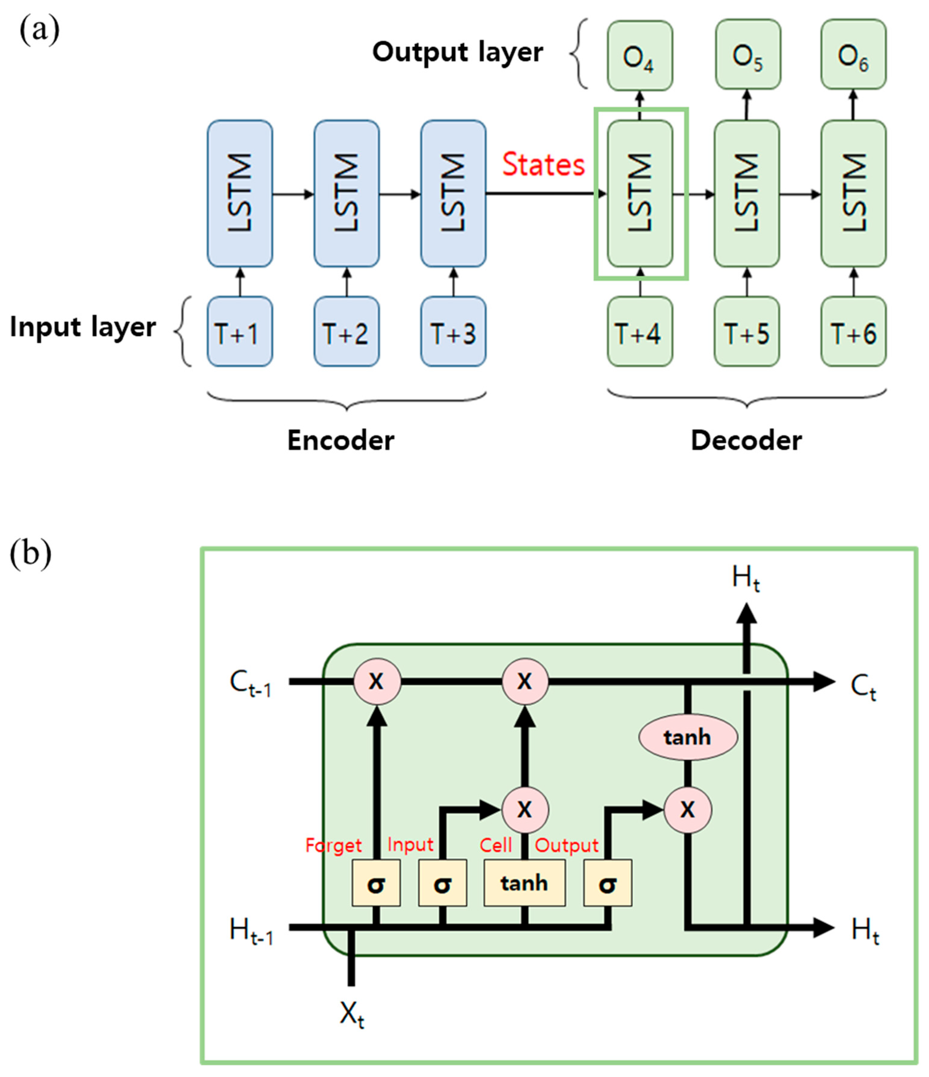

Table 2.
The configuration for CMAQ model in this study.
| CMAQ v5.0.2 Module | Option |
|---|---|
| Horizontal advection (ModHadv) | Hyamo |
| Vertical advection (ModVadv) | YAMO |
| Horizontal diffusion (ModHdiff) | Multiscale |
| Vertical diffusion (ModVdiff) | Eddy |
| Aerosol module (ModAero) | AERO5 |
| Gas-phase chemistry solver (ModChem) | EBI |
| Deposition velocity calculation (ModDepv) | M3dry |
| Cloud module (ModCloud) | RADM |
| Gas-phase chemistry mechanism (Mechanism) | SAPRC99 |
Table 3.
Volume of data for the LSTM model.
| Integrated Model Name | T3V19 | T5V21 | T6V22 |
|---|---|---|---|
| Target Region |
Seoul | ||
| Training Period | 2016 ~ 2018 (3 years) | 2016 ~ 2020 (5 years) | 2016 ~ 2021 (6 years) |
| Evaluation Period | 2019 (1 year) | 2021 (1 year) | 2022 (1 year) |
| Training Data number |
450 million | 760 million | 910 million |
| Forecasting period | January 2023 ~ March 2023 (3 months) | ||
3. Description of LSTM Model
3.1. LSTM Model for Forecasting PM2.5 Concentration
Long Short-Term Memory (LSTM) is a sophisticated neural network introduced by Hochreiter and Schmidhuber (1997). An LSTM structure consists of input, output, and forget gates, each of which performs an individual function. The forget gate selectively removes unnecessary information from the previous cell state:
The sigmoid function outputs values between 0 and 1 to determine information retention, where the 128-dimensional hidden state and input are concatenated as input.
The input gate selects information to update while generating new candidate values:
This study employs the sine function instead of tanh, leveraging its periodic characteristics to better model cyclical patterns in time-series data. The cell state combines selective forgetting and input:
Each element of the 128-dimensional cell state vector is independently updated, integrating long-term and short-term information.
The Output gate regulates the final output:
The output gate determines which portions of the cell state are output, generating the final hidden state through sine modulation. The model training employs the Backpropagation Through Time (BPTT) algorithm. To prevent overfitting, an early stopping technique is implemented to automatically terminate training when validation loss ceases to improve.
3.2. Model Evaluation
The performance statistics proposed by Emery et al. (2017) were used as the evaluation criteria. Emery et al. (2017) conducted a review of 38 peer-reviewed air quality modeling studies published in SCI-indexed journals and proposed criteria for evaluation of models using normalized mean bias (NMB), normalized mean error (NME), and the correlation coefficient (R). NMB indicates the degree to which model predictions systematically overestimate or underestimate, while a negative value indicates underestimation. NME measures the magnitude of the error by taking the absolute differences between predicted and observed values, with lower values indicating better model performance. R represents the strength and direction of the linear relationship between the predicted and observed values, ranging from -1 to 1.
According to Emery et al. (2017), the 33rd and 67th percentiles divide the overall distribution into three performance categories: studies within the 33rd quantile successfully meet the “goal” benchmarks that the best performing models are expected to achieve; studies between the 33rd and 67th quantiles successfully meet the “criteria” that the majority of modeling studies achieve; and studies that fall outside the 67th quantile indicate relatively poor performance for that specific metric. Emery et al., (2017) recommended evaluating model performance using normalized mean bias (NMB), normalized mean error (NME), and correlation coefficient (R). According to the “Goal” benchmarks, acceptable performance is defined as NMB ≤ 10 %, NME ≤ 35 %, and R ≥ 0.7. The “criteria” are defined as NMB ≤ 30 %, NME ≤ 50 %, and R ≥ 0.4. Root Mean Square Error (RMSE) is used to evaluate the overall error of model by comparing its forecasting data to observed data, which is used to measure the standard deviation of prediction error. RMSE is more sensitive to outliers and a lower RMSE implies the improvement of the model performance. IOA is a correlation-based measure of the differences between simulated and observed data in terms of the mean and variance. IOA varies between 0 and 1 with a value of 1 indicating a perfect match, and 0 no agreement at all.
Here, M and O represent the modeled and observed PM2.5 concentrations, respectively, and N denotes the total number of data points. This study evaluated the forecasted PM2.5 concentrations for D+0, D+1, and D+2.
4. Results
Evaluation of the overall performance of the LSTM models is conducted by assessing their D+0, D+1, and D+2 forecasting accuracy and comparing it with that of CMAQ over Seoul during the period from January 1 to March 30, 2023. The time series of daily forecasting and observed PM2.5 concentrations for the D+0, D+1, and D+2 are shown in Figure 4. All models are capable of accurately simulating the overall observed trend, but those trained on larger datasets tend to approximate the observed values more closely. The CMAQ results noticeably overestimate relative to the DL-model outputs across all lead times. The right panel of Figure 4 shows the differences between CMAQ, T3V19, T5V21, and T6V22-simulated and observed values. Like the PM2.5 concentration time series, the numerical model exhibits the largest difference, whereas the DL-based models show reduced differences as the data volume increases. In terms of predictive performance against CMAQ data, the three DL-based models (T3V19, T5V21, and T6V22) demonstrate more accurate forecasting performance over the entire forecasting period than CMAQ-based PM2.5 concentrations. This indicates that the DL-based models are capable of accurately exhibiting the characteristic rapid trends-both increases and decreases-in PM2.5 concentrations.
Figure 5 shows scatter plots of daily averaged PM2.5 concentration between observation and models across all lead times at Seoul. The DL-models achieved the best performance, particularly T6V22, with an R2 value of 0.75. The numerical model consistently overestimates PM2.5 concentration and shows limited ability to capture temporal patterns, which is indicated by its large regression slope. In contrast, the DL-based models demonstrate progressively improved pattern reproduction as the volume of the training dataset increases.
To evaluate the accuracy of CMAQ, T3V19, T5V21, and T6V22, Table 4 and Figure 6 present evaluation metrics for PM2.5 forecasting performance over a three-day (D+0, D+1, and D+2) period using five statistical metrics (R, IOA, NMB, NME, RMSE) in Seoul. The correlation coefficient evaluates how well the numerical and LSTM models represent the temporal trend of the observed values. The correlation coefficient (R) increases from 0.79 in the CMAQ model to 0.85 in the T6V22_6HR model.
The numerical model (CMAQ) records a Normalized Mean Bias (NMB) of 32.0%. This value exceeds the “Criteria” threshold of ±30% suggested by Emery et al. (2017) recommendations, which indicates low forecasting accuracy. When the training data covers three years, the NMB decreases to 23.8%. This value meets the Criteria threshold. When the data period extends to five years, the NMB drops sharply to 2.9%. This result is close to the “Goal” benchmark of ±10%. With six years of data, the NMB further decreases to 1.3%. This change results in approximately 96% improvement compared to the CMAQ model. The Normalized Mean Error (NME) decreases from 43.3% in the CMAQ model to 22.6% in the T6V22_6HR model. This reduction means that the prediction error becomes nearly half of its original value. RMSE, which penalizes large errors more heavily, shows the outstanding performance of the DL-models across all lead times compared to the numerical model. The RMSE values of the DL models range from5.7 to 11.1 , indicating up to 67.4% improvement over the numerical model. This suggests that the DL-models result in fewer large deviations from observed values than the numerical model. The Index of Agreement (IOA) also increases from 0.82 to 0.91. This change shows that the agreement between the predicted and observed values improves. These results confirm that the developed DL-based model shows better performance than the CMAQ model in Seoul in terms of overall accuracy. The expansion of the dataset improves all performance indicators. The improvements in NMB and NME are particularly significant.
5. Concluding Remarks
This study develops an LSTM-based PM2.5 prediction model for the Seoul area by integrating diverse observational data and numerical model data to overcome the limitations of CMAQ numerical models in PM2.5 forecasting, including high computational costs, emission inventory limitations, uncertainties in meteorological and chemistry assumptions, and enormous time requirements for numerical model improvements. The PM2.5 prediction model for the Seoul region is developed utilizing various meteorological and air quality observed data, numerical model outputs, and secondary variables.
Statistical evaluation shows that all LSTM models (T3V19, T5V21, T6V22) perform better than the conventional CMAQ model in terms of NMB, NME, and R across all lead times (D+0 to D+2). The CMAQ model shows relatively poor performance, with NMB ranging from 21.0% to 31.9%, NME from 39.9% to 45.3%, and R from 0.69 to 0.84 exceeding the “Criteria” thresholds for NMB (±30%) at D+1 and D+2. In contrast, the T3V19 meets the “Criteria” level, with NMB ranging from 23.8% to 26.4%, NME from 30.5% to 32.5%, and R from 0.86 to 0.92. The T5V21 and T6V22 satisfy “Goal” benchmarks (NMB ≤ ±10%, NME ≤ ±35%, R ≥ 0.7) across all lead times. Specifically, T5V21 shows NMB values between 2.9% and 8.6%, NME between 16.7% and 24.1%, and R between 0.83 and 0.94. T6V22 demonstrated the best performance, with NMB values between -0.2% and 3.7%, NME from 14.8% to 22.6%, and R values between 0.85 and 0.94. Compared to CMAQ, T6V22 reduced NMB by up to 96% and NME by up to 50%, demonstrating substantial improvement in forecast accuracy. These consistent results are maintained when lead time increases.
The LSTM model developed in this study can provide fast and accurate air quality forecast information to the public while compensating for the shortcomings of numerical models. Furthermore, given high-quality observational data and numerical model data continue to accumulate in the future, the performance of deep learning-based PM2.5 forecasting models is expected to be further enhanced. Future studies should focus on developing and evaluating models for various regions because each region has different characteristics of PM2.5. They should also assess the forecasting performance of the models over longer periods of ensure stability and accuracy.
Acknowledgments
This work was supported by a grant from the National Institute of Environmental Research (NIER), funded by the Ministry of Environment (MOE) of the Republic of Korea (NIER-2024-01-01-011).
Conflicts of Interest
The authors declare that they have no conflict of interest. (required).
References
- Bakels, L.; Tatsii, D.; Tipka, A.; Thompson, R.; Dütsch, M.; Blaschek, M.; Seibert, P.; Baier, K.; Bucci, S.; Cassiani, M.; et al. FLEXPART version 11: improved accuracy, efficiency, and flexibility. Geosci. Model Dev. 2024, 17, 7595–7627. [Google Scholar] [CrossRef]
- Baklanov, A.; Zhang, Y. Advances in air quality modeling and forecasting. Glob. Transitions 2020, 2, 261–270. [Google Scholar] [CrossRef]
- Baklanov, A.; Schlünzen, K.; Suppan, P.; Baldasano, J.; Brunner, D.; Aksoyoglu, S.; Carmichael, G.; Douros, J.; Flemming, J.; Forkel, R.; et al. Online coupled regional meteorology chemistry models in Europe: current status and prospects. Atmospheric Meas. Tech. 2014, 14, 317–398. [Google Scholar] [CrossRef]
- Chang, A. 2020. Cleaning and disinfectant chemical exposures and temporal associations with COVID-19—National poison data system, United States, January 1, 2020–March 31, 2020. MMWR. Morbidity and Mortality Weekly Report, 69.
- Chen, G.; Chen, S.; Li, D.; Chen, C. A hybrid deep learning air pollution prediction approach based on neighborhood selection and spatio-temporal attention. Sci. Rep. 2025, 15, 1–20. [Google Scholar] [CrossRef]
- Chen, Y.; Huang, L.; Xie, X.; Liu, Z.; Hu, J. Improved prediction of hourly PM2.5 concentrations with a long short-term memory and spatio-temporal causal convolutional network deep learning model. Sci. Total. Environ. 2023, 912, 168672. [Google Scholar] [CrossRef] [PubMed]
- Cheng, F.-Y.; Feng, C.-Y.; Yang, Z.-M.; Hsu, C.-H.; Chan, K.-W.; Lee, C.-Y.; Chang, S.-C. Evaluation of real-time PM2.5 forecasts with the WRF-CMAQ modeling system and weather-pattern-dependent bias-adjusted PM2.5 forecasts in Taiwan. Atmospheric Environ. 2021, 244. [Google Scholar] [CrossRef]
- Albuquerque, T.T.d.A.; Andrade, M.d.F.; Ynoue, R.Y.; Moreira, D.M.; Andreão, W.L.; dos Santos, F.S.; Nascimento, E.G.S. WRF-SMOKE-CMAQ modeling system for air quality evaluation in São Paulo megacity with a 2008 experimental campaign data. Environ. Sci. Pollut. Res. 2018, 25, 36555–36569. [Google Scholar] [CrossRef]
- Do, K.; Mahish, M.; Yeganeh, A.K.; Gao, Z.; Blanchard, C.L.; Ivey, C.E. Emerging investigator series: a machine learning approach to quantify the impact of meteorology on tropospheric ozone in the inland southern California. Environ. Sci. Atmos. 2023, 3, 1159–1173. [Google Scholar] [CrossRef]
- Emery, C.; Liu, Z.; Russell, A.G.; Odman, M.T.; Yarwood, G.; Kumar, N. Recommendations on statistics and benchmarks to assess photochemical model performance. J. Air Waste Manag. Assoc. 2017, 67, 582–598. [Google Scholar] [CrossRef]
- Ferreira, J.; Lopes, D.; Rafael, S.; Relvas, H.; Almeida, S.M.; Miranda, A.I. Modelling air quality levels of regulated metals: limitations and challenges. Environ. Sci. Pollut. Res. 2020, 27, 33916–33928. [Google Scholar] [CrossRef]
- Flemming, J.; Benedetti, A.; Inness, A.; Engelen, R.J.; Jones, L.; Huijnen, V.; Remy, S.; Parrington, M.; Suttie, M.; Bozzo, A.; et al. The CAMS interim Reanalysis of Carbon Monoxide, Ozone and Aerosol for 2003–2015. Atmos. Chem. Phys. 2017, 17, 1945–1983. [Google Scholar] [CrossRef]
- FLEXPART version 11 : improved accuracy, efficiency, and flexibility (2024).
- Fujino, R. and Miyamoto, Y., 2022. PM2.5 decrease with precipitation as revealed by single-point ground-based observation. Atmospheric Science Letters, 23(7), p.e1088.
- Gao, X. and Li, W., 2021. A graph-based LSTM model for PM2. 5 forecasting. Atmospheric Pollution Research, 12(9), p.101150. Yang, J. and Zhao, Y., 2023. Performance and application of air quality models on ozone simulation in China–A review. Atmospheric Environment, 293, p.119446.
- Gao, Z.; Zhou, X. A review of the CAMx, CMAQ, WRF-Chem and NAQPMS models: Application, evaluation and uncertainty factors. Environ. Pollut. 2023, 343, 123183. [Google Scholar] [CrossRef] [PubMed]
- Grell, G.A. , Peckham, S.E., Schmitz, R., McKeen, S.A., Frost, G., Skamarock, W.C. and Eder, B., 2005. Fully coupled “online” chemistry within the WRF model. Atmospheric environment, 39(37), pp.6957-6975.
- Hochreiter, S. & Schmidhuber, J. Long short-term memory. Neural Comput. 9(8), 1735–1780 (1997).
- Huang, L. , Zhu, Y., Zhai, H., Xue, S., Zhu, T., Shao, Y., Liu, Z., Emery, C., Yarwood, G., Wang, Y. and Fu, J., 2021. Recommendations on benchmarks for numerical air quality model applications in China–Part 1: PM 2.5 and chemical species. Atmospheric Chemistry and Physics, 21(4), pp.2725-2743.
- Jeong, D.; Yoo, C.; Yeh, S.-W.; Yoon, J.-H.; Lee, D.; Lee, J.-B.; Choi, J.-Y. Statistical Seasonal Forecasting of Winter and Spring PM2.5 Concentrations Over the Korean Peninsula. Asia-Pacific J. Atmospheric Sci. 2022, 58, 549–561. [Google Scholar] [CrossRef]
- Karimian, H.; Li, Q.; Wu, C.; Qi, Y.; Mo, Y.; Chen, G.; Zhang, X.; Sachdeva, S. Evaluation of Different Machine Learning Approaches to Forecasting PM2.5 Mass Concentrations. Aerosol Air Qual. Res. 2019, 19, 1400–1410. [Google Scholar] [CrossRef]
- Kumar, N.; Park, R.J.; Jeong, J.I.; Woo, J.-H.; Kim, Y.; Johnson, J.; Yarwood, G.; Kang, S.; Chun, S.; Knipping, E. Contributions of international sources to PM2.5 in South Korea. Atmospheric Environ. 2021, 261. [Google Scholar] [CrossRef]
- Li, N.; Zhang, H.; Zhu, S.; Liao, H.; Hu, J.; Tang, K.; Feng, W.; Zhang, R.; Shi, C.; Xu, H.; et al. Secondary PM2.5 dominates aerosol pollution in the Yangtze River Delta region: Environmental and health effects of the Clean air Plan. Environ. Int. 2022, 171, 107725. [Google Scholar] [CrossRef]
- Li, X.; Peng, L.; Yao, X.; Cui, S.; Hu, Y.; You, C.; Chi, T. Long short-term memory neural network for air pollutant concentration predictions: Method development and evaluation. Environ. Pollut. 2017, 231, 997–1004. [Google Scholar] [CrossRef] [PubMed]
- Li, Z. , Zhang, X., Liu, X. and Yu, B., 2022. PM2.5 pollution in six major Chinese urban agglomerations: spatiotemporal variations, health impacts, and the relationships with meteorological conditions. Atmosphere, 13(10), p.1696.
- Li, Z. , Zhang, X., Liu, X. and Yu, B., 2022. PM2.5 pollution in six major Chinese urban agglomerations: spatiotemporal variations, health impacts, and the relationships with meteorological conditions. Atmosphere, 13(10), p.1696.
- Ma, X.; Sha, T.; Wang, J.; Jia, H.; Tian, R. Investigating impact of emission inventories on PM2.5 simulations over North China Plain by WRF-Chem. Atmospheric Environ. 2018, 195, 125–140. [Google Scholar] [CrossRef]
- Park et al., Variation of PM2.5 Chemical Compositions and their Contributions to light extinction in Seoul, Aerosol and Air Quality Research, 18, 2220-2229, 2018.
- Park, E.H. , Heo, J., Hirakura, S., Hashizume, M., Deng, F., Kim, H. and Yi, S.M., 2018. Characteristics of PM 2.5 and its chemical constituents in Beijing, Seoul, and Nagasaki. Air Quality, Atmosphere & Health, 11, pp.1167-1178.
- Qadeer, K. , Rehman, W.U., Sheri, A.M., Park, I., Kim, H.K. and Jeon, M., 2020. A long short-term memory (LSTM) network for hourly estimation of PM2.5 concentration in two cities of South Korea. Applied Sciences, 10(11), p.3984.
- Retrieving ground-level PM2.5 concentrations in China (2013-2021) with a numerical-model-informed testbed to mitigate sample-imbalance-induced biases.
- Reyes-Villegas, E.; Lowe, D.; Johnson, J.S.; Carslaw, K.S.; Darbyshire, E.; Flynn, M.; Allan, J.D.; Coe, H.; Chen, Y.; Wild, O.; et al. Simulating organic aerosol in Delhi with WRF-Chem using the volatility-basis-set approach: exploring model uncertainty with a Gaussian process emulator. Atmospheric Meas. Tech. 2023, 23, 5763–5782. [Google Scholar] [CrossRef]
- Rybarczyk and Zalkeviciute, Machine Learning Approaches for Outdoor Air Quality Modelling: A Systematic Review (2018).
- Skamarock, W.C. , Klemp, J.B., Dudhia, J., Gill, D.O., Barker, D.M., Duda, M.G., Huang, X.Y., Wang, W. and Powers, J.G., 2008. A description of the advanced research WRF version 3. NCAR technical note, 475(125), pp.10-5065.
- Skamarock, W.C. , Klemp, J.B., Dudhia, J., Gill, D.O., Liu, Z., Berner, J., Wang, W., Powers, J.G., Duda, M.G., Barker, D.M. and Huang, X.Y., 2019. A description of the advanced research WRF model version 4. National Center for Atmospheric Research: Boulder, CO, USA, 145(145), p.550.
- Sokhi, R.S.; Moussiopoulos, N.; Baklanov, A.; Bartzis, J.; Coll, I.; Finardi, S.; Friedrich, R.; Geels, C.; Grönholm, T.; Halenka, T.; et al. Advances in air quality research – current and emerging challenges. Atmospheric Meas. Tech. 2022, 22, 4615–4703. [Google Scholar] [CrossRef]
- Statistical Seasonal Forecasting of Winter and Spring PM2.5 Concentrations over the Korean Peninsula, 2022, 58.
- Tao, H.; Xing, J.; Zhou, H.; Pleim, J.; Ran, L.; Chang, X.; Wang, S.; Chen, F.; Zheng, H.; Li, J. Impacts of improved modeling resolution on the simulation of meteorology, air quality, and human exposure to PM2.5, O3 in Beijing, China. J. Clean. Prod. 2020, 243. [Google Scholar] [CrossRef]
- Travis, K.R. , Crawford, J.H., Chen, G., Jordan, C.E., Nault, B.A., Kim, H., Jimenez, J.L., Campuzano-Jost, P., Dibb, J.E., Woo, J.H. and Kim, Y., 2022. Limitations in representation of physical processes prevent successful simulation of PM 2.5 during KORUS-AQ. Atmospheric Chemistry and Physics, 22(12), pp.7933-7958.
- Vignesh, P.P. , Jiang, J.H. and Kishore, P., 2023. Predicting PM2. 5 concentrations across USA using machine learning. Earth and Space Science, 10(10), p.e2023EA002911.
- Wang, P.; Qiao, X.; Zhang, H. Modeling PM2.5 and O3 with aerosol feedbacks using WRF/Chem over the Sichuan Basin, southwestern China. Chemosphere 2020, 254, 126735. [Google Scholar] [CrossRef] [PubMed]
- WHO Ambient Air Pollution: A Global Assessment of Exposure and Burden of Disease, 9789241511353 (2016) https://www.who.int/publications/i/item/9789241511353.
- Y. S. Kim, G. H. Y. S. Kim, G. H. Kwak, K. D. Lee, S. I. Na, C. W. Park, & N. W. Park: Performance Evaluation of Machine Learning and Deep Learning Algorithms in Crop Classification: Impact of Hyper-parameters and Training Sample Size. Korean Journal of Remote Sensing, 2018, 34(5), 811~827pp.
- Yu, M.; Cai, X.; Song, Y.; Wang, X. A fast forecasting method for PM2.5 concentrations based on footprint modeling and emission optimization. Atmospheric Environ. 2019, 219. [Google Scholar] [CrossRef]
- Zhang, H. , Wang, J., García, L.C., Zhou, M., Ge, C., Plessel, T., Szykman, J., Levy, R.C., Murphy, B. and Spero, T.L., 2022. Improving surface PM2. 5 forecasts in the United States using an ensemble of chemical transport model outputs: 2. Bias correction with satellite data for rural areas. Journal of Geophysical Research: Atmospheres, 127(1), p.e2021JD035563.
- Zhou, L.; Sun, L.; Luo, Y.; Xia, X.; Huang, L.; Liao, Z.; Yan, X. Air pollutant concentration trends in China: correlations between solar radiation, PM2.5, and O3. Air Qual. Atmosphere Heal. 2023, 16, 1721–1735. [Google Scholar] [CrossRef]
Figure 1.
The study area with WRF-CMAQ domain for 27 km horizontal grid. The red dots donate observed sites (25) of air quality in Seoul.
Figure 1.
The study area with WRF-CMAQ domain for 27 km horizontal grid. The red dots donate observed sites (25) of air quality in Seoul.
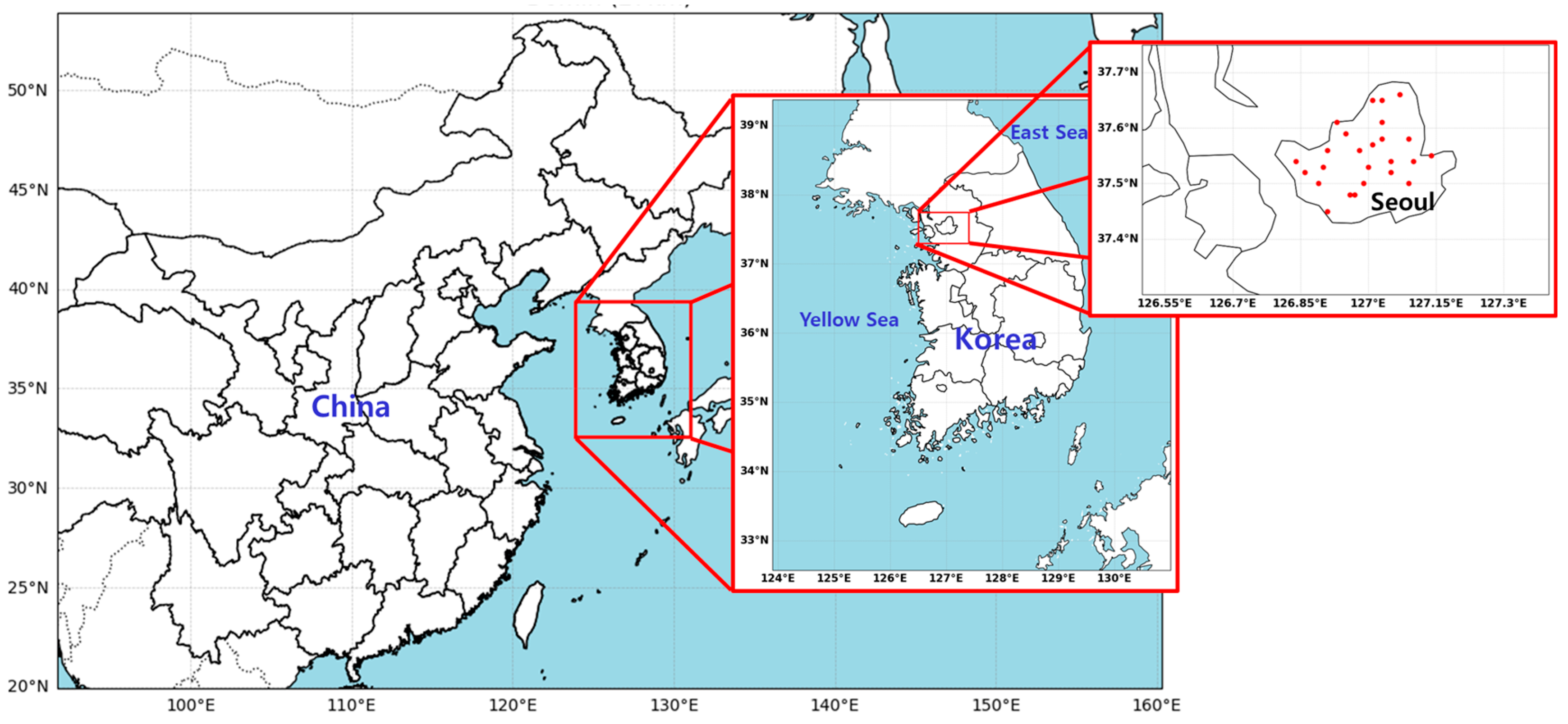
Figure 2.
Flowchart of the training process of the PM2.5 The network structure diagram of LSTM.
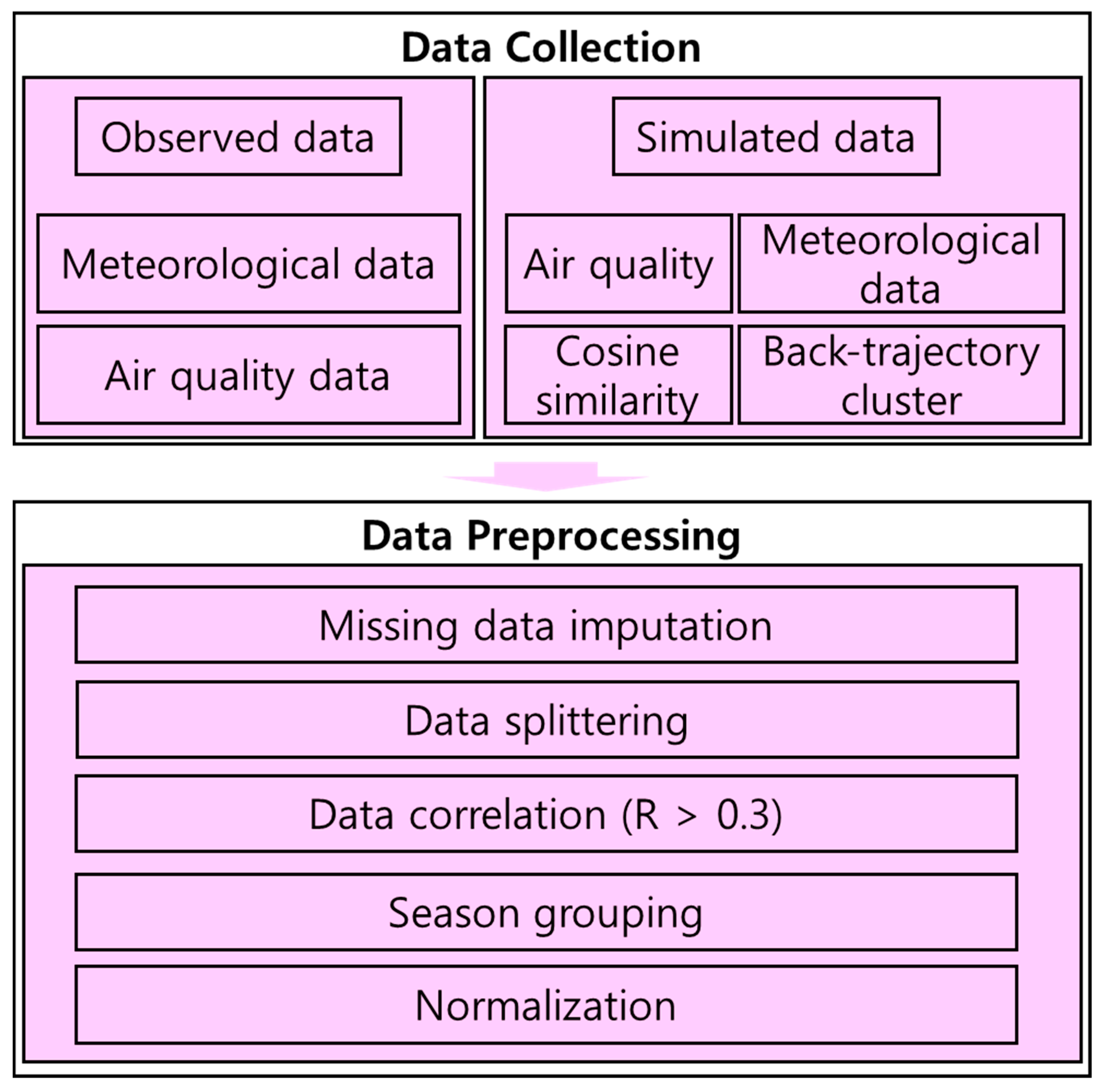
Figure 4.
Time series of daily PM2.5 concentration over 25 sites in Seoul from January and March 2023. The shaded gray (left) represents observational PM2.5 concentration while the blue, green, orange, and red represent PM2.5 concentrations of CMAQ, T3V19, T5V21, and T6V22. The dashed lines denote ‘bad’ and ‘very bad’ grades.
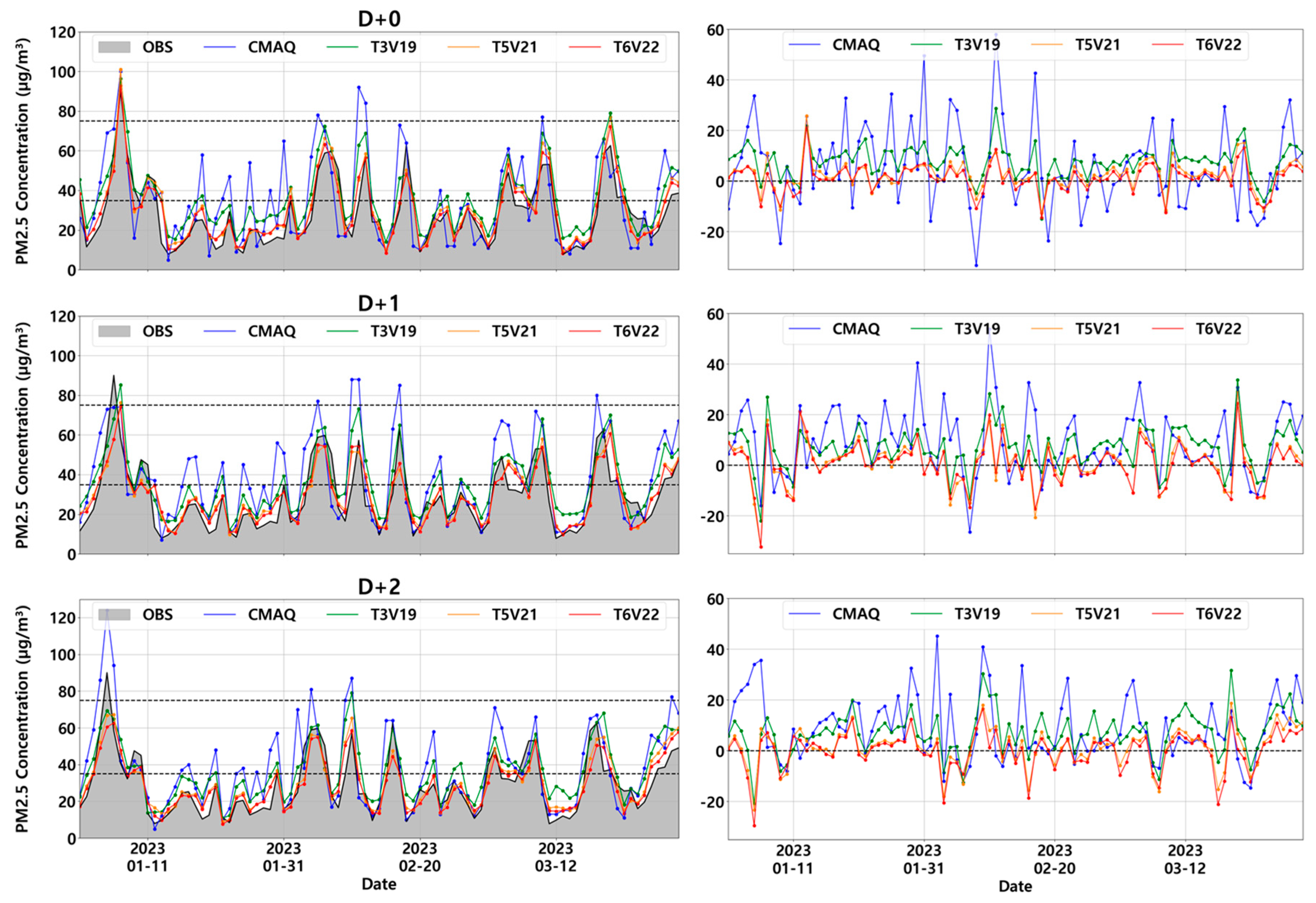
Figure 5.
The scatter plots between CMAQ, T3V19, T5V21, and T6V22 and observed data for PM2.5 concentrations in Seoul during all lead time (D+0, D+1, and D+2). The black dash lines indicate slope.
Figure 5.
The scatter plots between CMAQ, T3V19, T5V21, and T6V22 and observed data for PM2.5 concentrations in Seoul during all lead time (D+0, D+1, and D+2). The black dash lines indicate slope.
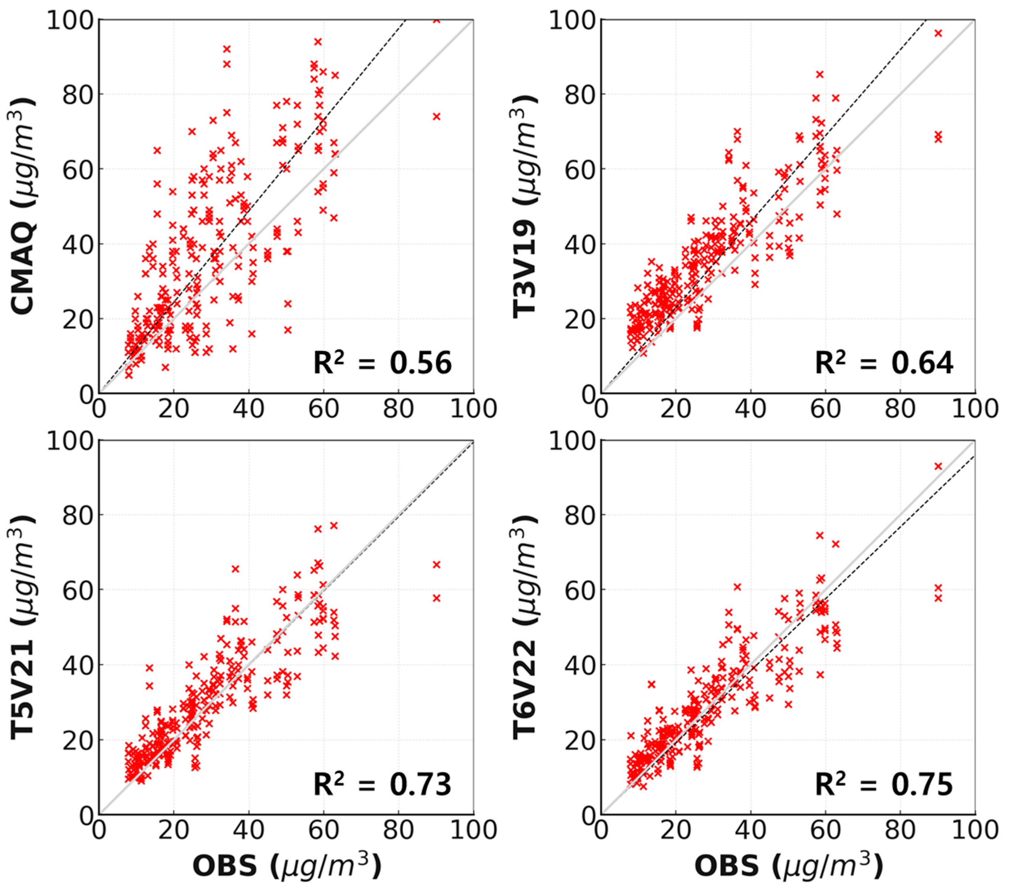
Figure 6.
Radar chart of D+0, D+1, and D+2 for R, NMB, NME, RMS, and IOA in Seoul.
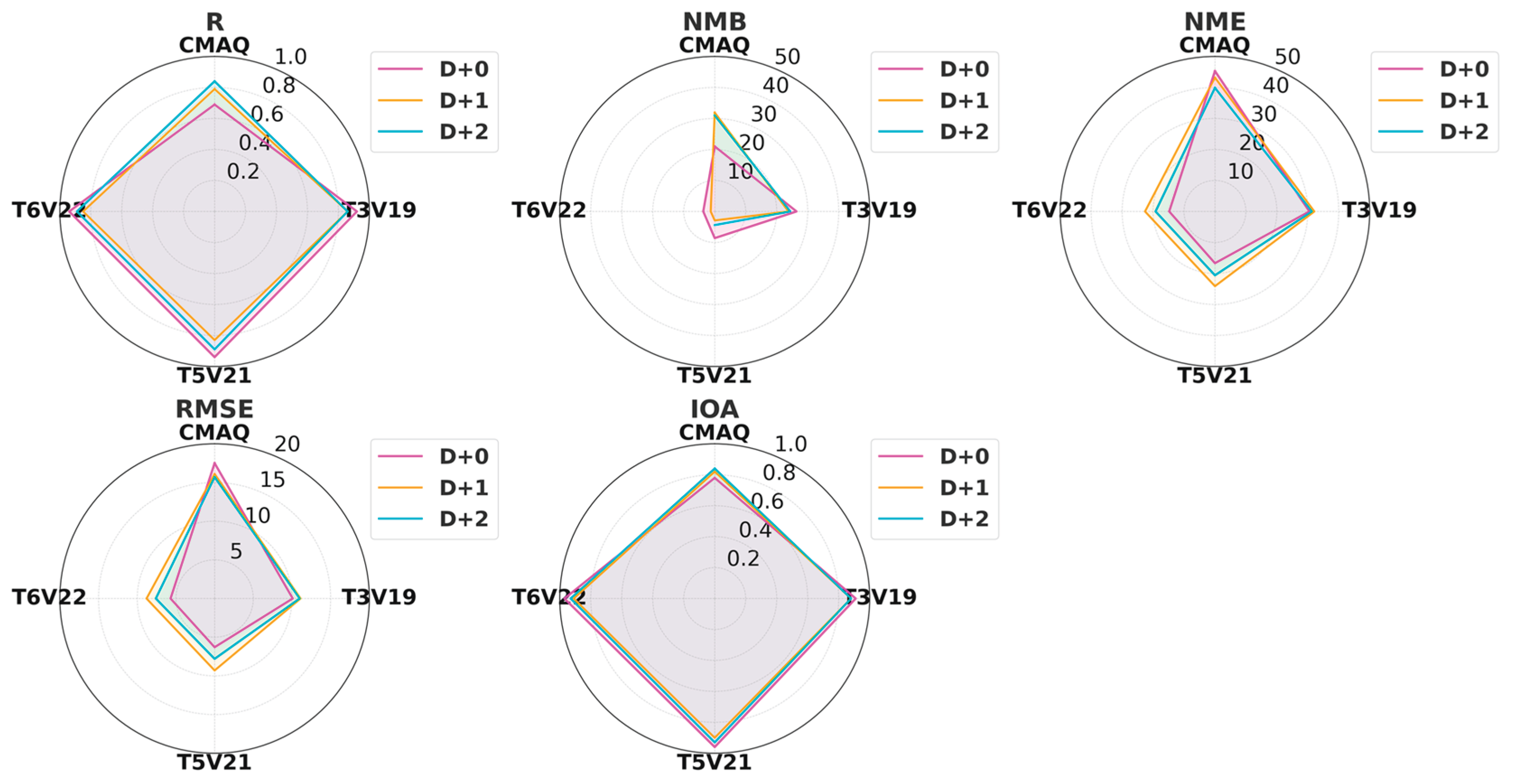
Table 1.
Variables of training and validation data for the LSTM model.
| Data Type | Variable | |
|---|---|---|
| Observation | Meteorological Variables (surface) |
Temperature (K), Dew point (K), Wind component (U, V; m/s), Sea level pressure (hPa), Precipitation (mm), Solar radiation (W/m2) |
| Air Quality variables | PM10 (μg/m3), PM2.5 (μg/m3), O3 (ppm), NO2 (ppm), CO (ppm), SO2 (ppm) | |
| Numerical data | Meteorological Variables (surface) |
Temperature (K), Dew point (K), Wind component (U, V; m/s), Sea level pressure (hPa), Precipitation (mm), Solar radiation (W/m2) |
| Meteorological Variables (925 hPa, 850 hPa, 700 hPa, 500 hPa) |
Temperature (K), , Relative humidity (%), Wind component (U, V; m/s), Geopotential height (m) | |
| Air Quality variables | PM10 (μg/m3), PM2.5 (μg/m3), O3 (ppm), NO2 (ppm), CO (ppm), SO2 (ppm) | |
| Back trajectory pattern | Local wind group, Northwestern wind group, Western wind group, Northern wind group, Short flow | |
| • Cosine Similarity (1000 hPa, 925 hPa, 850 hPa, 700 hPa, 500 hPa, 300 hPa) |
Temperature (K), Relative humidity (%), Wind components (U, V; m/s), Geopotential height (m) | |
Table 4.
Performance comparison of the 5 different evaluation measures between T3V19 T5V21, and T6V22-based PM2.5 prediction models for daily PM2.5 predictions.
Table 4.
Performance comparison of the 5 different evaluation measures between T3V19 T5V21, and T6V22-based PM2.5 prediction models for daily PM2.5 predictions.
| Forecast Lead Time | Models | R | NMB (%) | NME (%) | RMSE | IOA |
|---|---|---|---|---|---|---|
| D+0 | CMAQ | 0.69 | 21.0 | 45.3 | 17.5 | 0.78 |
| T3V19 | 0.92 | 26.4 | 30.5 | 10.1 | 0.91 | |
| T5V21 | 0.94 | 8.6 | 16.7 | 6.3 | 0.96 | |
| T6V22 | 0.94 | 3.7 | 14.8 | 5.7 | 0.97 | |
| D+1 | CMAQ | 0.79 | 31.9 | 43.2 | 16.1 | 0.82 |
| T3V19 | 0.86 | 23.8 | 32.1 | 11.1 | 0.88 | |
| T5V21 | 0.83 | 2.9 | 24.1 | 9.3 | 0.90 | |
| T6V22 | 0.85 | 1.3 | 22.6 | 8.8 | 0.91 | |
| D+2 | CMAQ | 0.84 | 31.0 | 39.9 | 15.7 | 0.84 |
| T3V19 | 0.86 | 24.4 | 31.3 | 11.1 | 0.88 | |
| T5V21 | 0.89 | 4.4 | 20.6 | 7.8 | 0.93 | |
| T6V22 | 0.89 | -0.2 | 19.2 | 7.6 | 0.93 |
Disclaimer/Publisher’s Note: The statements, opinions and data contained in all publications are solely those of the individual author(s) and contributor(s) and not of MDPI and/or the editor(s). MDPI and/or the editor(s) disclaim responsibility for any injury to people or property resulting from any ideas, methods, instructions or products referred to in the content. |
© 2025 by the authors. Licensee MDPI, Basel, Switzerland. This article is an open access article distributed under the terms and conditions of the Creative Commons Attribution (CC BY) license (http://creativecommons.org/licenses/by/4.0/).
Copyright: This open access article is published under a Creative Commons CC BY 4.0 license, which permit the free download, distribution, and reuse, provided that the author and preprint are cited in any reuse.


