
Submitted:
21 June 2025
Posted:
23 June 2025
You are already at the latest version
Abstract
Pests that live on mango leaves are bad for both the safety of our food and the growth of our business. It is most common for powdery mildery, golmachi, bacterial canker, and anthracnose to be found on mango leaves in Bangladesh. If these illnesses are caught early, they can make people more productive. However, this can't be done quickly and correctly by hand. This study suggests a method that uses CNN and transfer learning to find infections before they can spread. The data set came from the Mango farm and several fields. Our goal is to quickly and accurately find mango diseases so that they can help the growing business and save farmers a lot of time and work. It was ResNet50, MobileNetV2, DenseNet201, MobileNetV3, and VGG16 that we used as transfer learning models. We used different activation functions, like elu and ReLu, as well as sigmoid and softmax functions for the thick layer to sort the model into groups. Based on the f1 Score, accuracy, memory, and precision, the suggested way is a better model than the current models. Among this model, the ResNet50 model provided better results, with 96.49% accuracy.
Keywords:
Mango
; Neural Network
; deep learning
; Image Recognition
; Convolutionary Neural Network (CNN)
Introduction
Mango trees are a key source of food and have a major role in protecting wildlife. In the farming field, the “mango” is becoming a popular fruit. One of the largest widely grown and important crops in terms of trade is the mango. Bangladesh is the world’s seventh-largest mango grower. Mangoes are important to the success of our nation’s economy. But there is an issue. Mango trees occasionally become sick. Because the mangoes don’t grow well and are tough to sell, this could be harmful to the farmers. Among these, diseases that target Mango leaves have the ability to greatly impact both the amount and quality of the yield. As we all know, mangoes are also a great source of calcium, magnesium, folate, choline, vitamin A, vitamin C, and vitamin K. According to a Food and Agriculture Organization (FAO) study, By 2050, it is expected that there will be 9.1 billion people on the world., needing approximately 70% growth in food production to ensure a steady supply (Golhani et al., 2018). Plants must be shielded from illness in order to grow high-quality food. Mangoes face a range of illnesses throughout their lives. This paper covers different mango leaf illnesses and their signs, such as Golmachi, Powdery Mildew, Bacterial Canker, and Anthracnose. Illnesses in mango leaves need to be properly and quickly discovered in order to avoid yield losses and handle diseases effectively. When plant illnesses were first found, plant tracking was usually done on a daily basis by knowledgeable farmers. For tiny farms, it was possible to It is simple to spot the illnesses and to take prompt preventative and control action. However, big farms take a lot of time to finish and costly. Plant death comes from illnesses that hinder photosynthesis and affect the growth of the plant. This work’s main goal is to spot mango leaf diseases using a few well-known CNN models. Mango leaf disease identification with convolutional neural network models is one of four disease kinds that are used for classification. CNNs, or convolutional neural networks, have grown into incredibly powerful tools for picture recognition and classification (Rashed & kakon, 2025). These deep-learning models are helpful for studying plant diseases using pictures of leaves because they are very good at spotting small patterns and characteristics in images. CNNs have the ability to greatly increase the speed, accuracy, and scalability of the testing process when used to spot illnesses in mango leaves. This study aims to explore and apply a CNN- based method Regarding the automatic identification of illnesses affecting mango leaves. The suggested way involves putting the CNN model through training with a collection of numerous shots of mango leaves, both healthy and broken. As a result, a way for finding plant illnesses in their very early stages is important. For this reason, I hope that the work I’ve shared will be helpful to mango fruit farmers and scholars.
Literature Review
In this article (Arivazhagan & Ligi, 2018), the early and accurate identification of five mango leaf diseases is automated with a noteworthy 96.67% accuracy to Convolutional Neural Network (CNN) utilization model. The model’s success shows how well it may be applied in real- time scenarios, which might be very advantageous for large-scale farms looking to improve disease control. Ongoing attempts to improve stability and limits in the model’s capacity to adapt to different external situations. In order to improve farming output, There is use of machine learning and computer vision in this article (Singh et al., 2019) Introducing the MCNN model for Anthracnose detection in Mango leaves. MCNN offers computing efficiency and beats current methods with an amazing accuracy of 97.13%. Investigating different activation functions is one of the next directions. resolving inconsistent information in real time.
In this study (Maheshwari & Shrivastava, 2020), a deep learning method for automatic mango Using convolutional neural networks (CNNs) to identify leaf disease is suggested with the goal of improving food quality. The work handles the threat to plant health, especially in mango plants, and helps find answers to the global warming problem.
This paper (Patil et al., 2022) gets accuracies ranging from 94% to 98% by using ResNet models in a transfer learning approach for mango leaf disease detection. ResNet-18’s 98% success rate led to its selection. The suggested way makes it easier to spot leaf diseases quickly and effectively, which helps farms make choices.
This study (Krishnamoorthy et al., 2021), uses CNN and transfer learning to spot illnesses of rice plants. There are 5200 pictures in their collection. The pictures were gathered from several online sites, including Kaggle. Pictures of three diseases that affect rice leaves: bacterial blight, leaf blast, and brown spot —as well as healthy leaves are included in the collection. With a basic CNN model and some parameter tweaking, They succeeded in getting an accuracy of 84.75%. They made use of transfer learning and the InceptionResNetV2 model. There were 3000 cases in the test set and 4000 instances in the training set. They got a 95.67% success rate.
It was made clear in this study (Khan et al., 2021), that they were able to spot rose illnesses based only on pictures of roses. Rose disease, however, cannot be a good treatment because the results would be terrible if the tree already has a particular illness. In their work, they have used MobileNet to perform transfer learning. In their study, they even got a hopeful result of 95.63% accuracy. To identify the different plant species, this study (Ghazi et al., 2017), mixed the utilizing a deep convolutional neural network as a transfer learning method. They applied three fearsome deep learning brickwork scilicets: GoogleNet, AlexNet, and VGGNet. The accuracy of the combination method improved to an average 80%. The Mobilenetv2 pre-trained model was used as a method for feature extraction in this article (Moyazzoma et al., 2021) to suggest a transfer learning approach for spotting plant leaf diseases. This method split the leaves into two groups: disease-affected and disease-free, with a confirmation accuracy of 90.80%. In this study (Rizvee et al., 2023), models such as AlexNet and VGG16 are beaten by LeafNet, a CNN-based model created for early diagnosis of mango diseases in tropical South Asia, with an average accuracy of 98.55%. With its high accuracy, memory, F-score, and specificity—all of which were taught on a special dataset from Bangladesh LeafNet has the ability to improve mango output and ease financial problems. In this study (Khan et al., 2023) originally split the pictures in order to find Rose Leaf Disease. After that, they got a color distribution using the k-means grouping method. Furthermore, by calculating the difference between the color of the pixels and the picture weights, they have inferred smart edge recognition after spreading the pixels. In the end, they labeled the disease using CNN. Although the datasets’ labels and correctness are unknown in this work, the method appears to be very good, thus we will follow this line of research. A CNN-based model for finding carrot diseases was presented in this study (Methun et al., 2021) Four different types of carrot diseases are included, and a collection of healthy carrots is also made. Recall, accuracy, precision, and f1 score are familiar to compare the performance of the proposed model with the current model; however, a ROC curve and AUC value are missing to show which part of the suggested model works well. Inception V3 offers better accuracy in this suggested model, at 97.4%.
Convolutional neural networks were applied in this study (Gandhi et al., 2018), to identify the various plant disease kinds. They implement Generative Adversarial Networks, or GANs, in order to improve their picture collection. They apply two CNN-based models: MobileNet and Inception v3. When using Inception V3, they obtain an accuracy of 88.6%, and when using the MobileNet model, they obtain a 92% accuracy.
| Author Name | Methodology | Description | Outcome |
| Rahman et al., 2025 | CNN and transfer Learning | Using deep neural networks and transfer learning to predict rice diseases | 99% |
| Salauddin et al., 2025 | Convolutional Neural Networks | tomato leaf diseases detection based on CNN | 95.37% |
| Our proposed model | CNN with Transfer learning | Mango leaf diseases detection based on CNN | 96.49% |
Materials and Methods
This study works on finding diseases in mango leaves to help farmers improve earnings. A big collection of mango leaf pictures was taken from farms to examine different situations. Using transfer learning, we applied deep learning models like ResNet-50, VGG19, MobileNetV2, MobileNetV3, and DenseNet201. The images were divided into four categories: healthy and three cancer types. The models were tested using accuracy, loss, and performance plots. Among them, our method got high accuracy, showing the usefulness of these techniques.
Data Collection
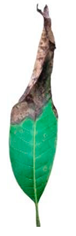
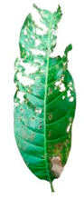
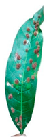
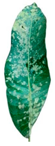
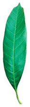
We gathered 998 mango leaf photos from different sources, including a mango farm, using a mobile camera. The collection includes five classes: healthy, golmachi, bacterial canker, anthracnose, and powdery mildew. These pictures were used to build a model capable of spotting four diseases and distinguishing them from healthy leaves.
Five characteristics are found in the collected information. Powdery mildery, Healthy, golmachi, bacterial canker, and anthracnose are the traits. The datasets for training and exams have been broken split into two separate parts, Every one including the dataset. A selection of the various training samples is kept for confirmation. Below are some examples of the dataset’s images:

Table 01.
Samples of the dataset’s images.
 |
 |
 |
 |
 |
| Anthracnose | Bacterial canker | Golmachi | Powdery mildew | Healthy |
Data Preprocessing
We changed the dataset such that certain low-resolution and fuzzy photos could be used in the study. After carefully reviewing the information, we removed any pictures that did not meet the minimum level of quality. We changed the picture sizes a little.
Statistical Analysis
There were 998 pictures in our collection, split into 5 categories. Several pictures shown earlier and the Index of Classes for each among those five Classes are shown below.
Table 02.
Class index for each of those five classes.
| Class Name | Class Index | No. of Images |
|---|---|---|
| powdery_mildery | 0 | 200 |
| Healthy | 1 | 200 |
| golmachi | 2 | 198 |
| bacterial_canker | 3 | 200 |
| anthracnose | 4 | 200 |
Proposed Methodology
For transfer learning, we applied VGG-19, MobileNetV2, ResNet-50, MobileNet-V3, and DesNet-201. For every model, we used different training and test files. The training dataset was used to build the training set and test set. After that, the models received training and preparation for the rating.
ResNet-50
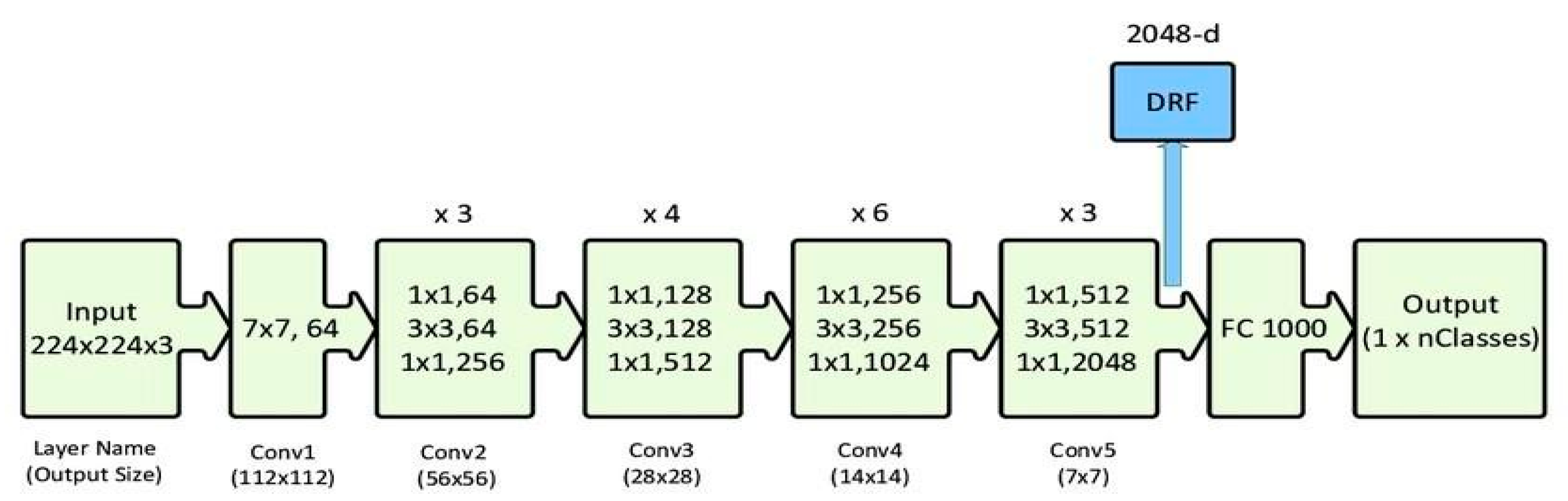
We used the ResNet-50 model to identify healthy and sick mango leaves. The collection of 998 images across five classes was trimmed to 224x224 pixels and standardized. Images were split into training and confirmation sets. Using transfer learning with Keras, ResNet-50 was applied to lower computing cost and training time. The model was trained and tested over multiple epochs, with accuracy and loss displayed using Matplotlib. Once learned, estimates on new pictures were made using OpenCV after cropping. This process showed the usefulness of transfer learning in disease classification.
Figure 01.
Sample Architecture model of ResNet-50.
VGG-19
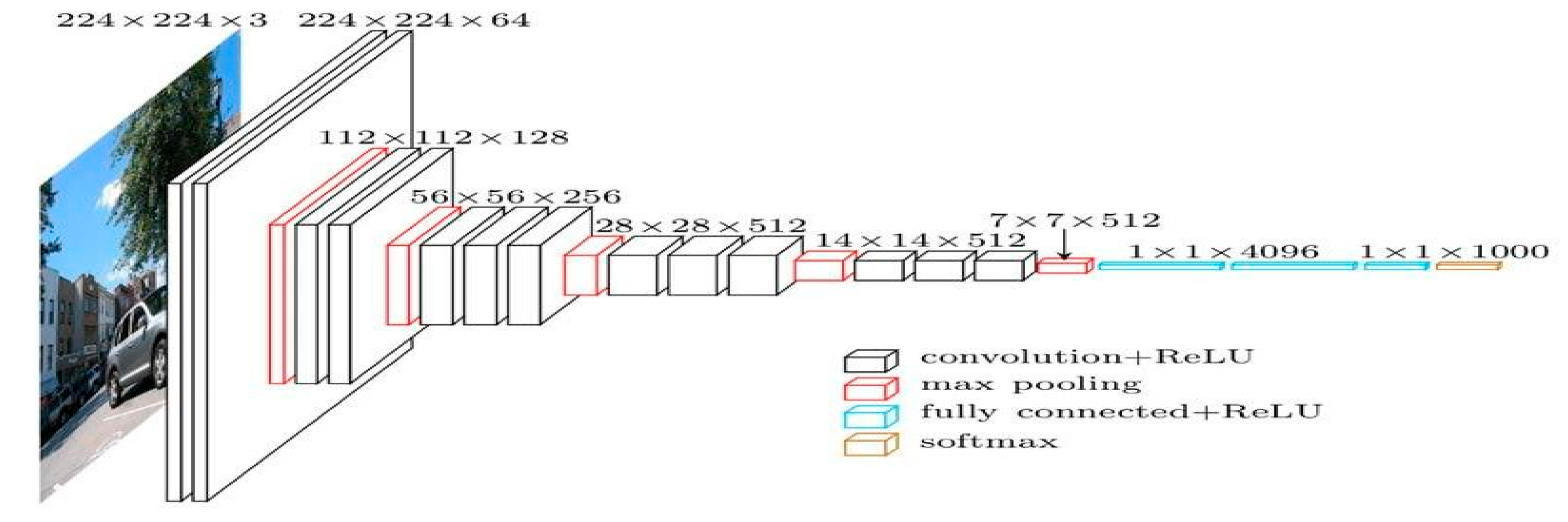
In this work, we have employed VGG19 in combination with Resnet-50 to spot dangerous pictures separately from healthy pictures by utilizing several layers and methods. The VGG19 model uses a 224 224 picture as its input, which has three channels, each of which has had its mean RGB value removed. Three fully connected (fc) layers and sixteen convolutional layers make up the model’s 19 weighted layers. In the VGG design, layers for 2D Convolution and Max Pooling form each block. However, the network’s depth has been further improved by adding a convolutional layer to the last three blocks. In addition to other VGG models, Keras has a special preparation method for VGG19. Getting the pretrained net is the last step in the training process, which starts with getting the resources. Next, in order to perform basic uses, we must group pictures, create a list of the available features of the expected object, Determine the chance of the ten most likely things that the net projected. This stops the accurate recognition of an object that is not of the ImageNet class. Next, you’ll need to get the names of every class that is being offered. The last three layers of the network must be erased to allow the skilled network to create an image’s vector representation. Once this is done, a group of shots and Put the traits of a group of pictures into a graphic style. We will take the first convolutional layer’s weights from the training net. The next step is to build a classifier using the test and training sets along with the pre-trained mode. The linear layer of the pre-trained net should be removed. The pretrained net should be at the top of our new net, followed by linear layers and softmax layers. If perfect accuracy is achieved on the test set, look up the total number of factors for each array online. Obtain the whole set of data. After that, an overview picture must be presented, along with the full list of factors and the numbers of the different types of levels.
Figure 03.
Sample Architecture model of VGG-19.
MobileNet-V2
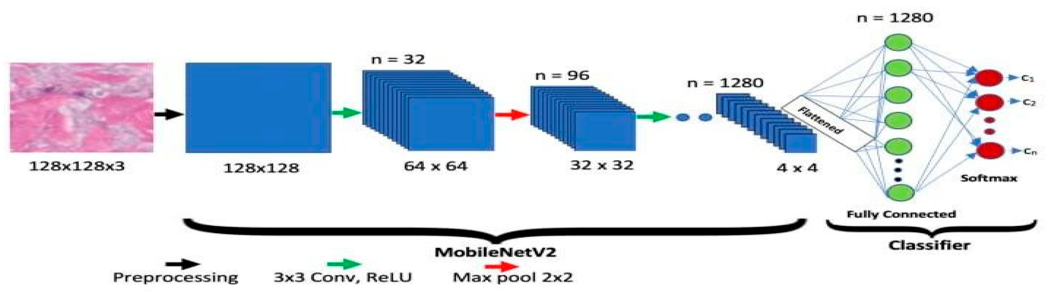
The Google group has approved MobileNet-V2. Two different types of blocks are present in it, each along with three levels. Eleven convolutional layers are present in each block, the first, second, and third having 32 filters each. Longitudinal bottlenecks between layers are important to limit the amount of data that non-linearity can influence. Block 2 has a step of two, whereas Block 1 has one. Each block has a unique pace.
Figure 04.
Sample Architecture model of MobileNet-V2.
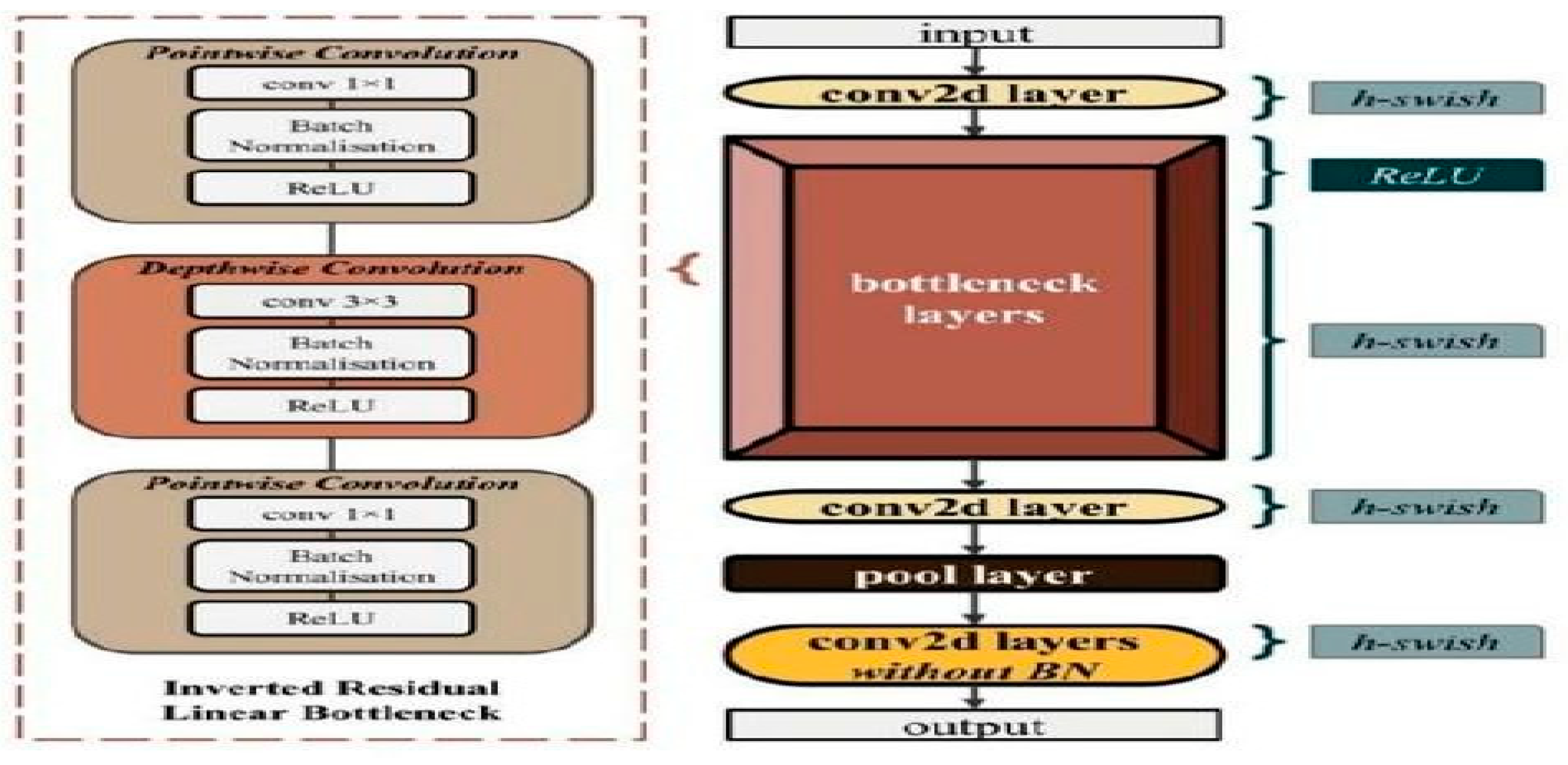
MobileNet-V3
With the help of the Net Adapt algorithm and hardware-aware network architecture search (NAS), A convolutional neural network called MobileNetV3 is tuned for CPUs in mobile phones. It is then further improved by new advancements in building. The 28- layer MobileNetV3 model uses hard-swish activation and batch normalization after the convolution layers.
Figure 05.
Sample Architecture model of MobileNet-V3.
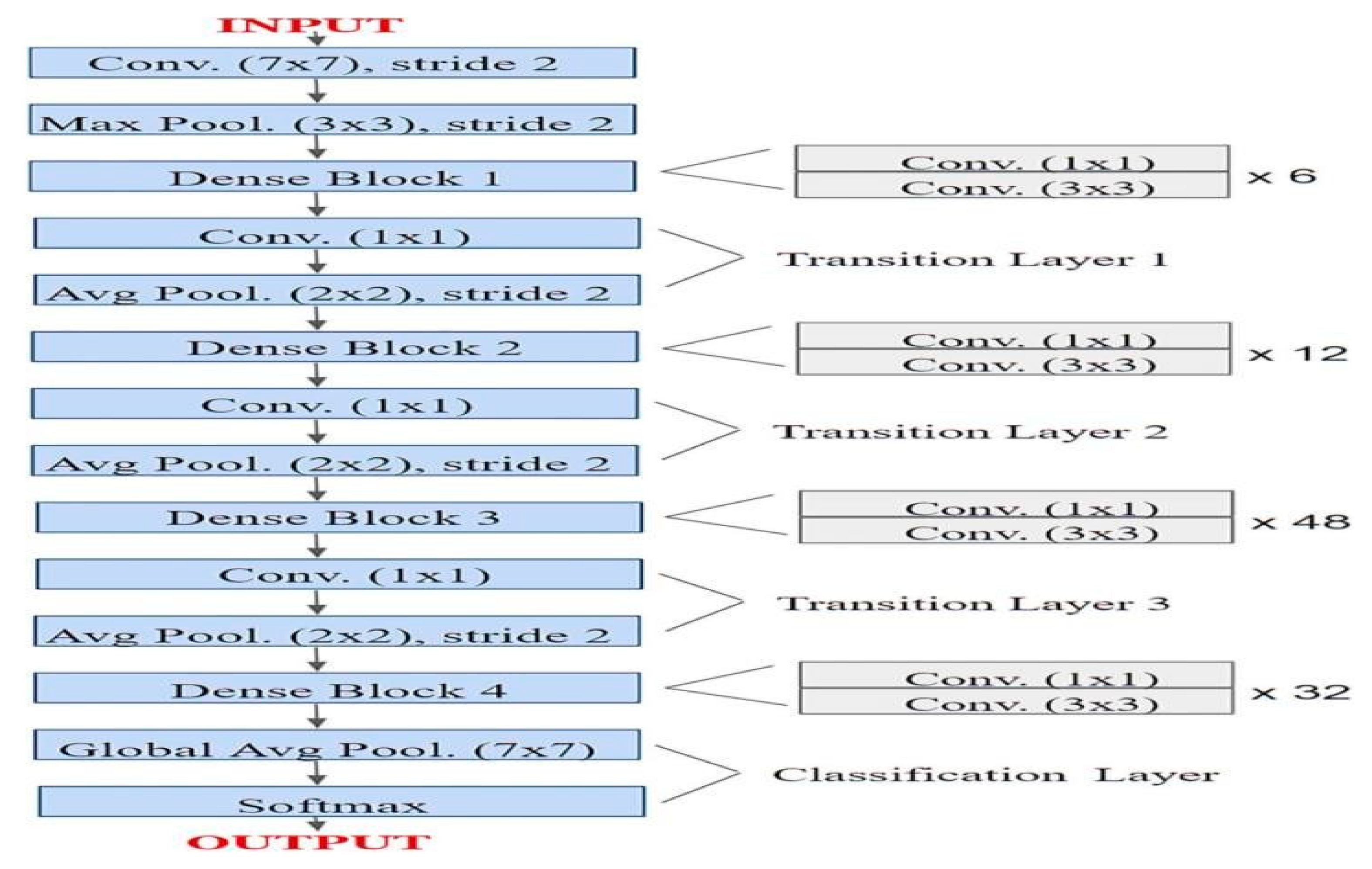
DenseNet-201
DenseNet-201 is a 201-layer convolutional neural network pretrained on the ImageNet collection with over a million pictures. It can recognize more than 1,000 object types, allowing it to learn diverse and complex traits. The network allows input pictures of 224x224 pixels, making it perfect for transfer learning in image classification tasks like mango leaf disease detection.
Figure 06.
Sample Architecture model of DenseNet-201.
Results and Discussion
We built our neural network using the transfer learning method. Five different transfer learning methods were put forth by us. such as MobileNetV2, ResNet50, VGG-19, and MobileNetV3 and DenseNet201
Table 03.
Accuracy comparison of several Model.
| Pre-trained Models | Test Accuracy |
|---|---|
| ResNet-50 | 96.49% |
| VGG-19 | 87% |
| MobileNet-v2 | 86.50% |
| MobileNet-v3 | 89% |
| DenseNet201 | 95.49% |
In this instance, ResNet50 fared better than those models, attaining an accuracy of 96.49%.
Figure 12 shows the training and evaluation accuracy/loss for the ResNet50 model. The blue line represents training ability, while the orange line shows evaluation results. Figure 07 shows the confusion matrix, showing that most illnesses were properly identified. However, some misclassifications happened — e.g., powdery_mildery was twice mistaken as golmachi, and healthy was mixed with powdery_mildery and golmachi. Despite these small mistakes, total performance was good. The Precision, Recall, and F1-score measures show the model’s high precision, with class names 0 to 4 representing powdery_mildery, healthy, golmachi, bacterial_canker, and anthracnose respectively.
Table 04.
ResNet50’s Classification report.
| Precision | Recall | F1-score | Support | |
|---|---|---|---|---|
| 0 | 0.93 | 0.95 | 0.94 | 40 |
| 1 | 1.00 | 0.93 | 0.96 | 40 |
| 2 | 0.91 | 0.97 | 0.94 | 40 |
| 3 | 1.00 | 1.00 | 1.00 | 40 |
| 4 | 1.00 | 0.97 | 0.99 | 40 |
| Accuracy | 0.96 | 200 | ||
| Macro avg | 0.97 | 0.97 | 0.97 | 200 |
| Weighted avg | 0.97 | 0.96 | 0.97 | 200 |
Figure 13 shows the training and evaluation accuracy/loss for the MobileNetV2 model. The blue lines show training measures, while the orange lines indicate evaluation results. Figure 08 shows the confusion matrix, showing that MobileNetV2 misclassified several data. For instance, powdery_mildery was often forecast as golmachi, and healthy leaves were mixed with powdery_mildery and golmachi. Similarly, anthracnose was mistaken as golmachi and bacterial_canker. Overall, the model failed compared to ResNet-50. Precision, Recall, and F1-score numbers show lower classification accuracy, with class names 0 to 4 representing powdery_mildery, healthy, golmachi, bacterial_canker, and anthracnose respectively.
Table 05.
MobileNetV2 Classification report.
| Precision | Recall | F1-score | Support | |
|---|---|---|---|---|
| 0 | 0.79 | 0.82 | 0.80 | 40 |
| 1 | 1.00 | 0.80 | 0.89 | 40 |
| 2 | 0.71 | 0.88 | 0.79 | 40 |
| 3 | 0.93 | 1.00 | 0.96 | 40 |
| 4 | 0.97 | 0.82 | 0.89 | 40 |
| Accuracy | 0.86 | 200 | ||
| Macro avg | 0.88 | 0.86 | 0.87 | 200 |
| Weighted avg | 0.88 | 0.86 | 0.87 | 200 |
Figure 14 shows the training and validation accuracy/loss for the VGG-19 model, where blue lines represent training data and orange lines indicate validation data. Figure 09 shows the confusion matrix, showing bad classification ability. Notable mistakes include misclassifying golmachi as powdery_mildery (11 times), and several healthy samples as powdery_mildery or golmachi. Powdery_mildery and anthracnose were also mixed. Overall, the model did significantly worse than ResNet-50. Precision, Recall, and F1-score measures confirm this, with labels 0 to 4 representing powdery_mildery, healthy, golmachi, bacterial_canker, and anthracnose respectively.
Table 06.
VGG-19 Classification report.
| Precision | Recall | F1-score | Support | |
|---|---|---|---|---|
| 0 | 0.69 | 0.95 | 0.80 | 40 |
| 1 | 1.00 | 0.80 | 0.89 | 40 |
| 2 | 0.89 | 0.62 | 0.74 | 40 |
| 3 | 0.93 | 1.00 | 0.96 | 40 |
| 4 | 0.93 | 0.97 | 0.95 | 40 |
| Accuracy | 0.87 | 200 | ||
| Macro avg | 0.89 | 0.87 | 0.87 | 200 |
| Weighted avg | 0.89 | 0.87 | 0.87 | 200 |
Figure 15 shows the training and validation accuracy/loss for the MobileNetV3 model, with blue lines showing training measures and orange lines indicating validation results. Figure 10 shows the confusion matrix, showing several misclassifications. For example, powdery_mildery was mixed with healthy, golmachi, and bacterial_canker; healthy leaves were misclassified as powdery_mildery and golmachi; and anthracnose was often forecast as golmachi. Overall, the model did worse than ResNet-50. The Precision, Recall, and F1-score numbers indicate this, with labels 0 to 4 corresponding to powdery_mildery, healthy, golmachi, bacterial_canker, and anthracnose respectively.
Table 07.
MobileNetV3 Classification report.
| Precision | Recall | F1-score | Support | |
|---|---|---|---|---|
| 0 | 0.82 | 0.80 | 0.81 | 40 |
| 1 | 0.97 | 0.85 | 0.91 | 40 |
| 2 | 0.77 | 0.93 | 0.84 | 40 |
| 3 | 0.93 | 0.97 | 0.95 | 40 |
| 4 | 1.00 | 0.90 | 0.95 | 40 |
| Accuracy | 0.89 | 200 | ||
| Macro avg | 0.90 | 0.89 | 0.89 | 200 |
| Weighted avg | 0.90 | 0.89 | 0.89 | 200 |
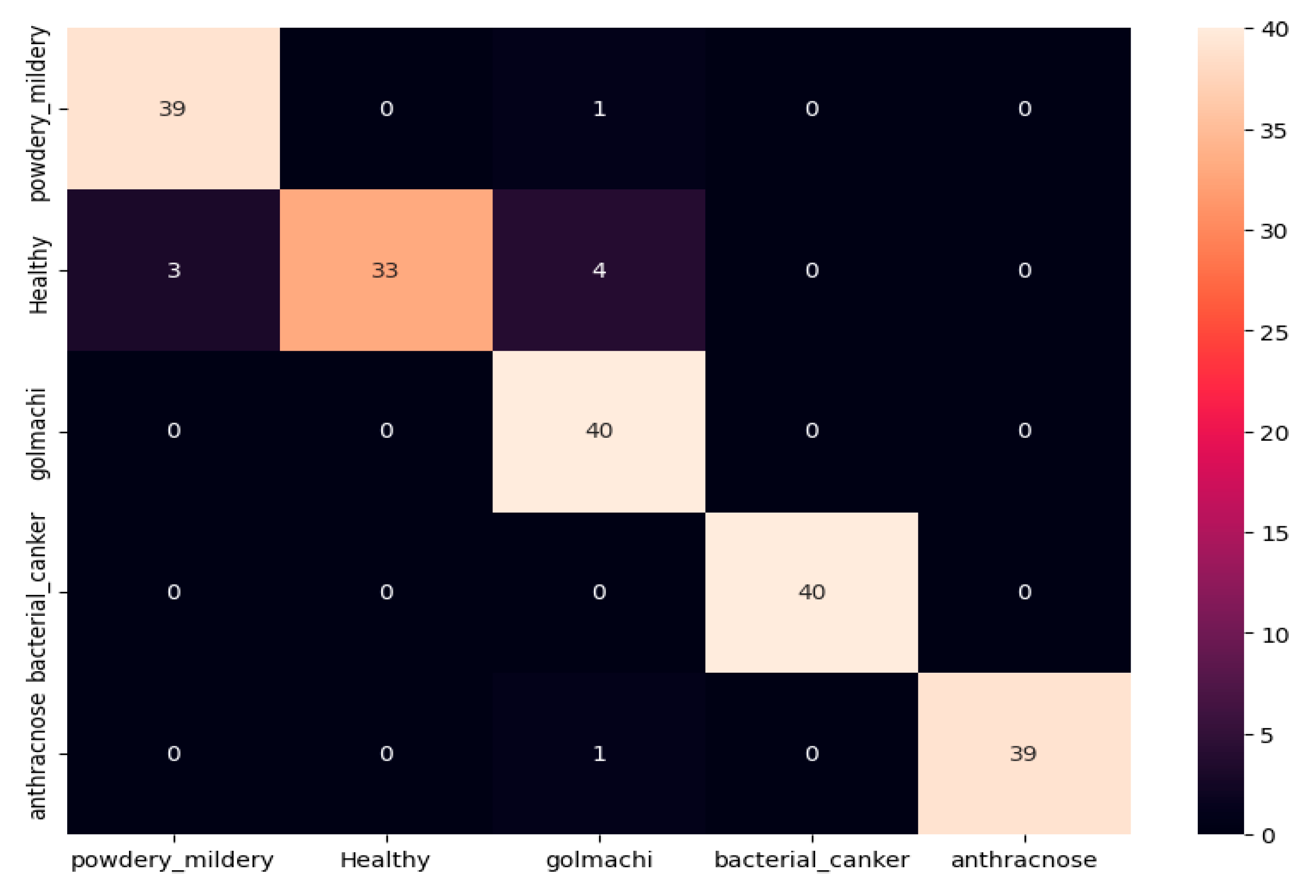
Figure 16 shows the training and evaluation accuracy/loss for the DenseNet201 model. Blue lines show training measures, while orange lines represent validation data. Figure 11 shows the confusion matrix, showing several misclassifications—such as powdery_mildery identified as golmachi, and healthy samples mislabeled as powdery_mildery or golmachi. Anthracnose was also confused with golmachi. Overall, DenseNet201 did not perform as well as ResNet-50. Precision, Recall, and F1-score results support this, with class names 0 to 4 representing powdery_mildery, healthy, golmachi, bacterial_canker, and anthracnose respectively.
Table 08.
DenseNet201 Classification report.
| Precision | Recall | F1-score | Support | |
|---|---|---|---|---|
| 0 | 0.93 | 0.97 | 0.95 | 40 |
| 1 | 1.00 | 0.82 | 0.90 | 40 |
| 2 | 0.87 | 1.00 | 0.93 | 40 |
| 3 | 1.00 | 1.00 | 1.00 | 40 |
| 4 | 1.00 | 0.97 | 0.99 | 40 |
| Accuracy | 0.95 | 200 | ||
| Macro avg | 0.96 | 0.95 | 0.95 | 200 |
| Weighted avg | 0.96 | 0.95 | 0.95 | 200 |
Confusion Metrix
The confusion matrix can be used to gauge how well classification models are working. The amount of info that we properly and wrongly identify is obvious. Thus, the following is my five models’ confusion matrix:
Figure 07.
Confusion Matrix of ResNet50.
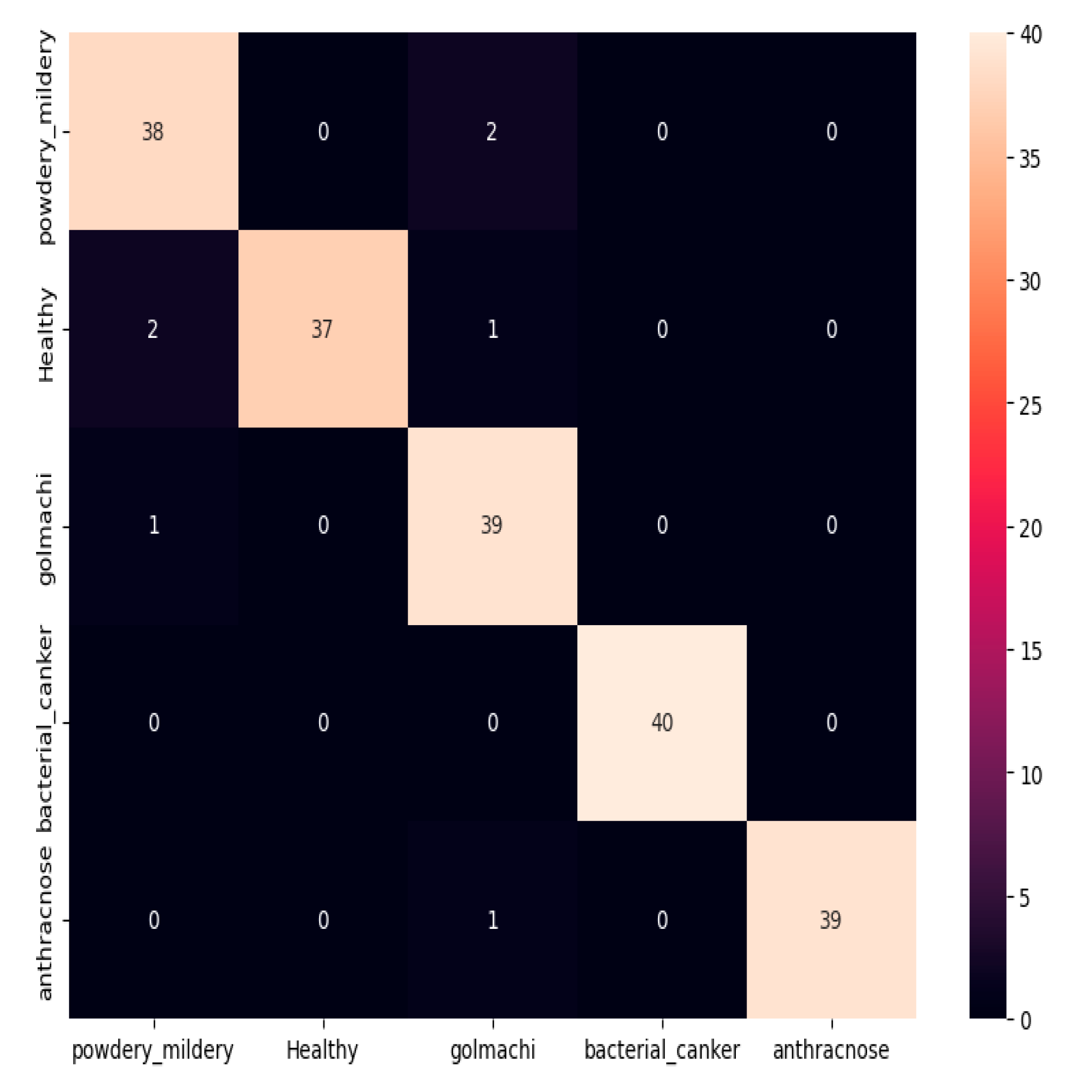
Figure 08.
Confusion Matrix of MobileNetV2.
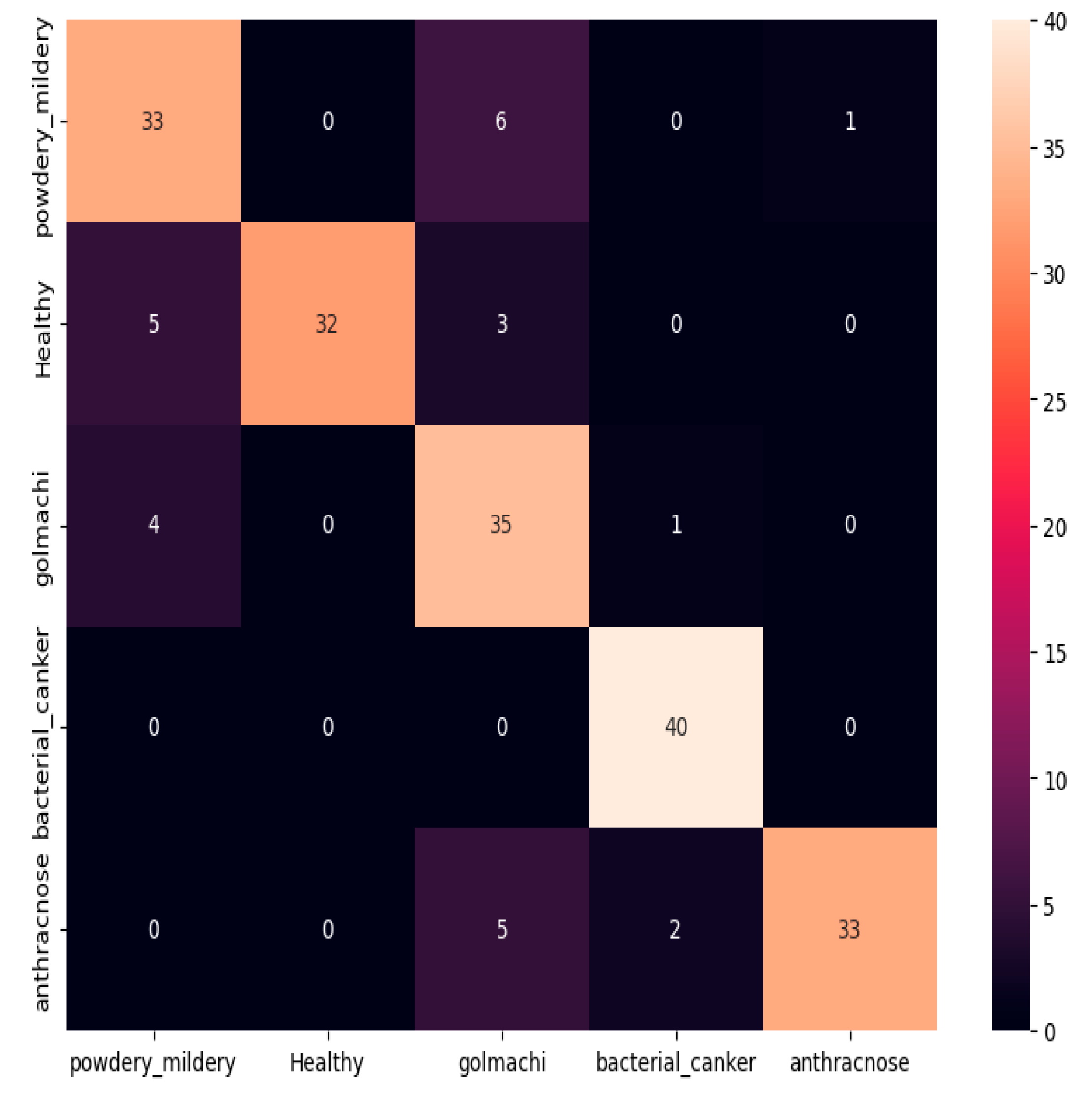
Figure 09.
Confusion Matrix of VGG-19.
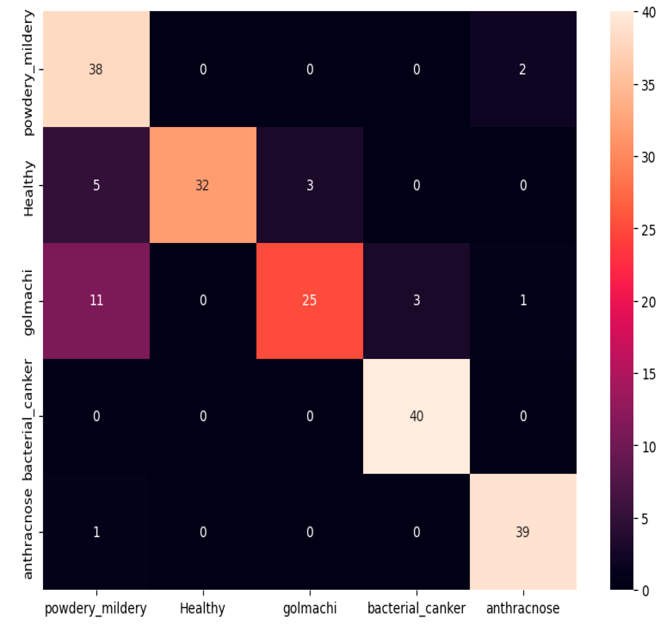
Figure 10.
Confusion Matrix of MobileNetV3.
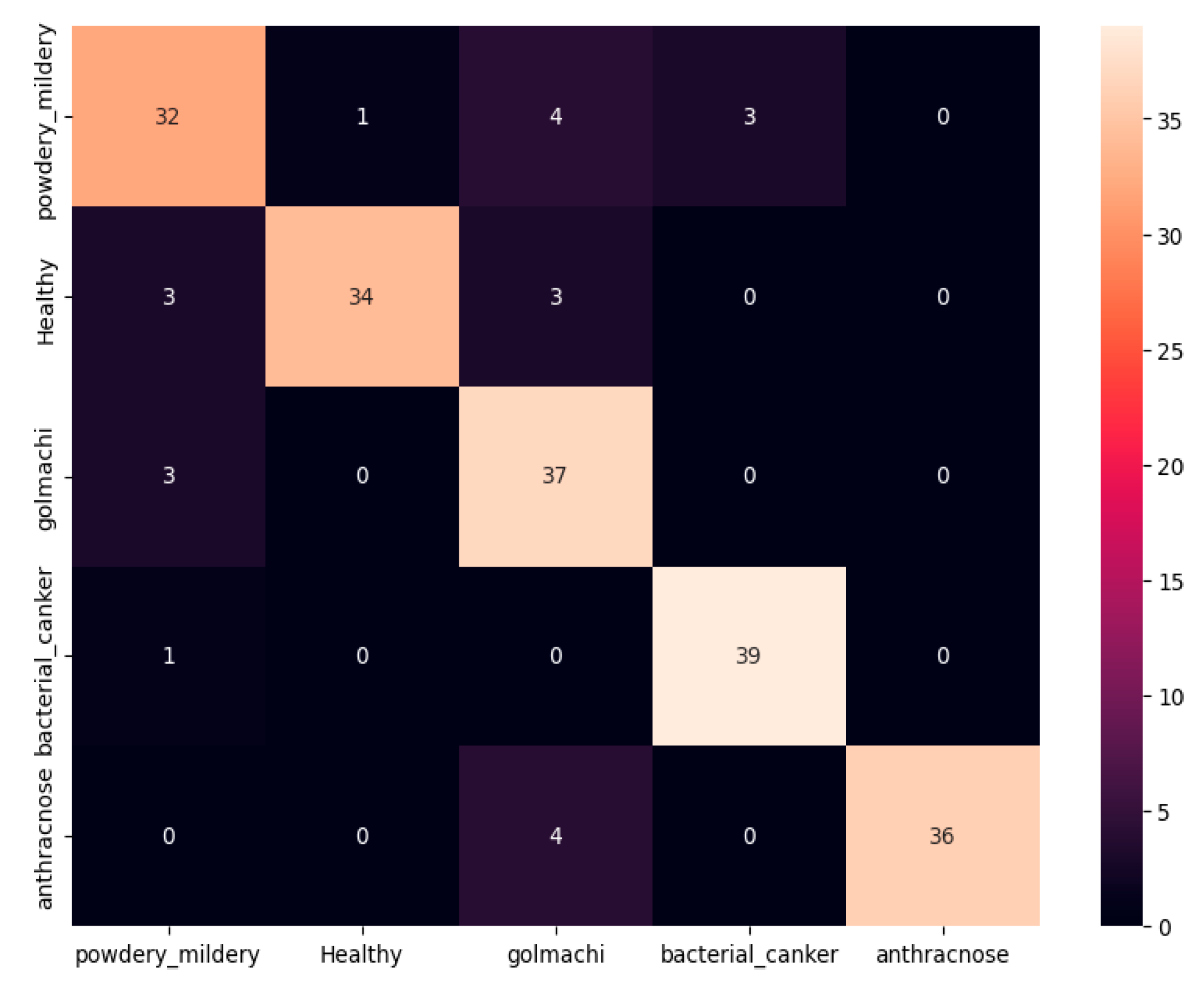
Figure 11.
Confusion Matrix of DenseNet201.
- Model Evolution
Figure 12.
ResNet50 Training-Validation Loss and Accuracy.
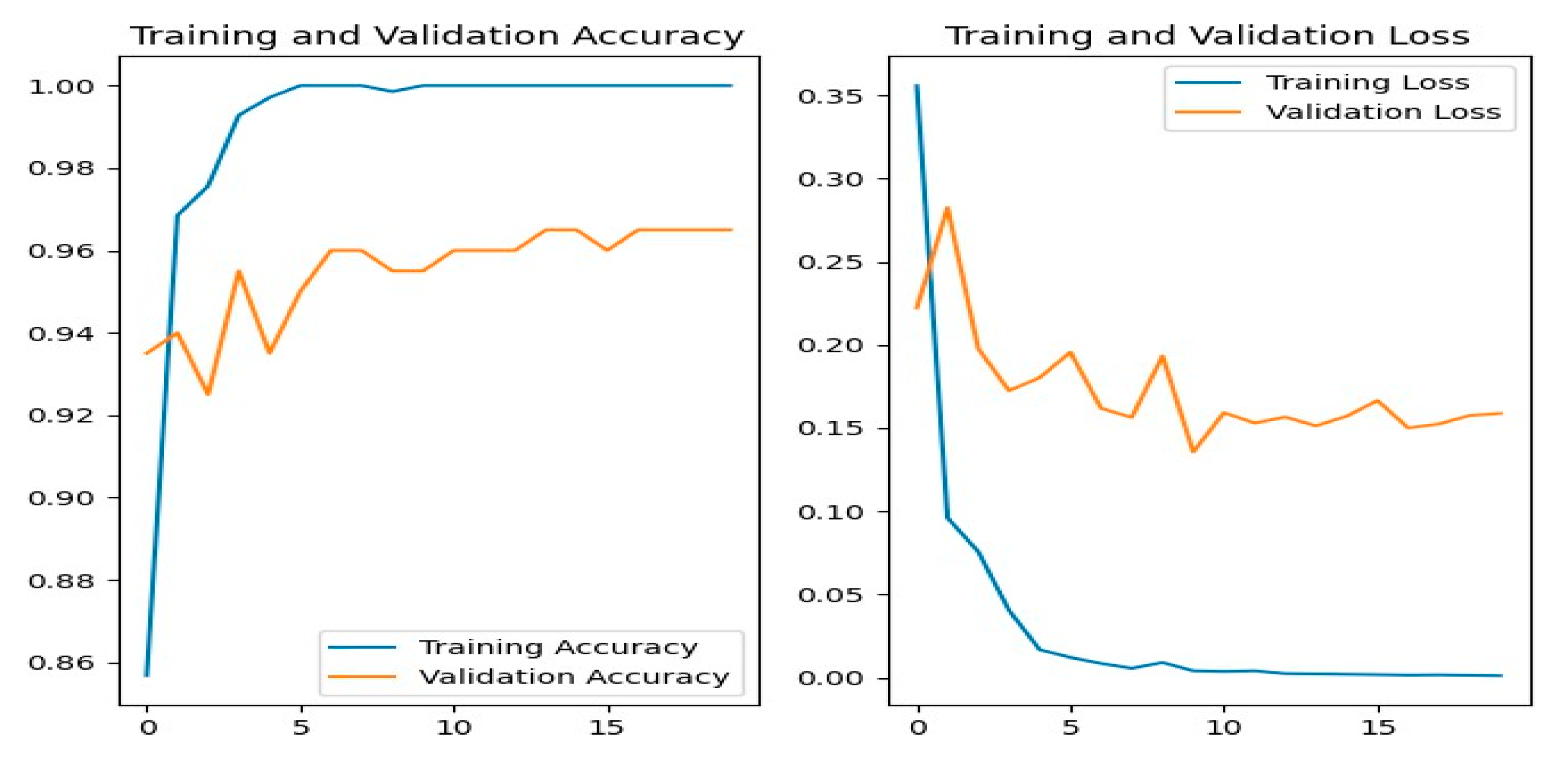
Figure 13.
MobileNetV2 Training-Validation Loss and Accuracy.
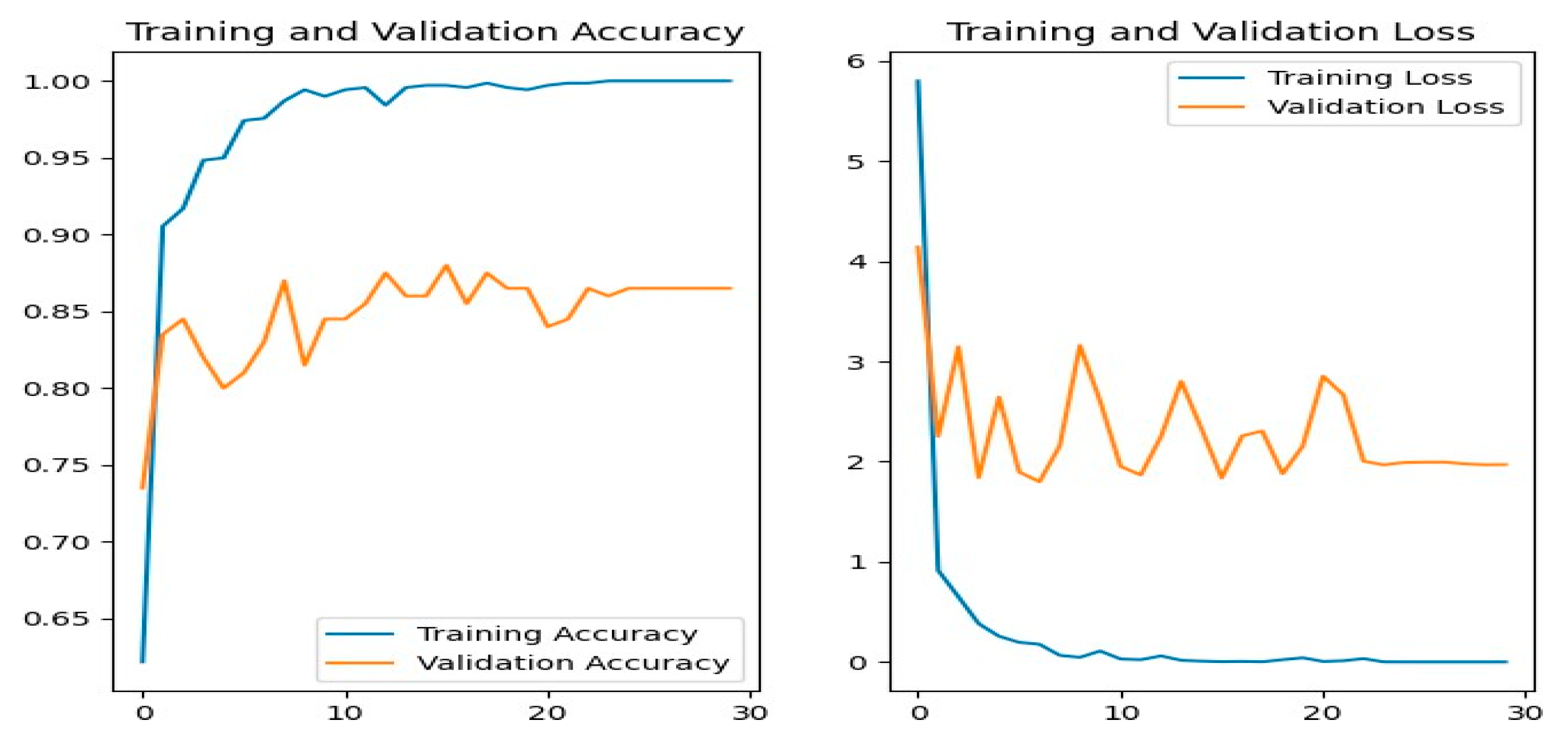
Figure 14.
VGG-19 Training-Validation Loss and Accuracy.
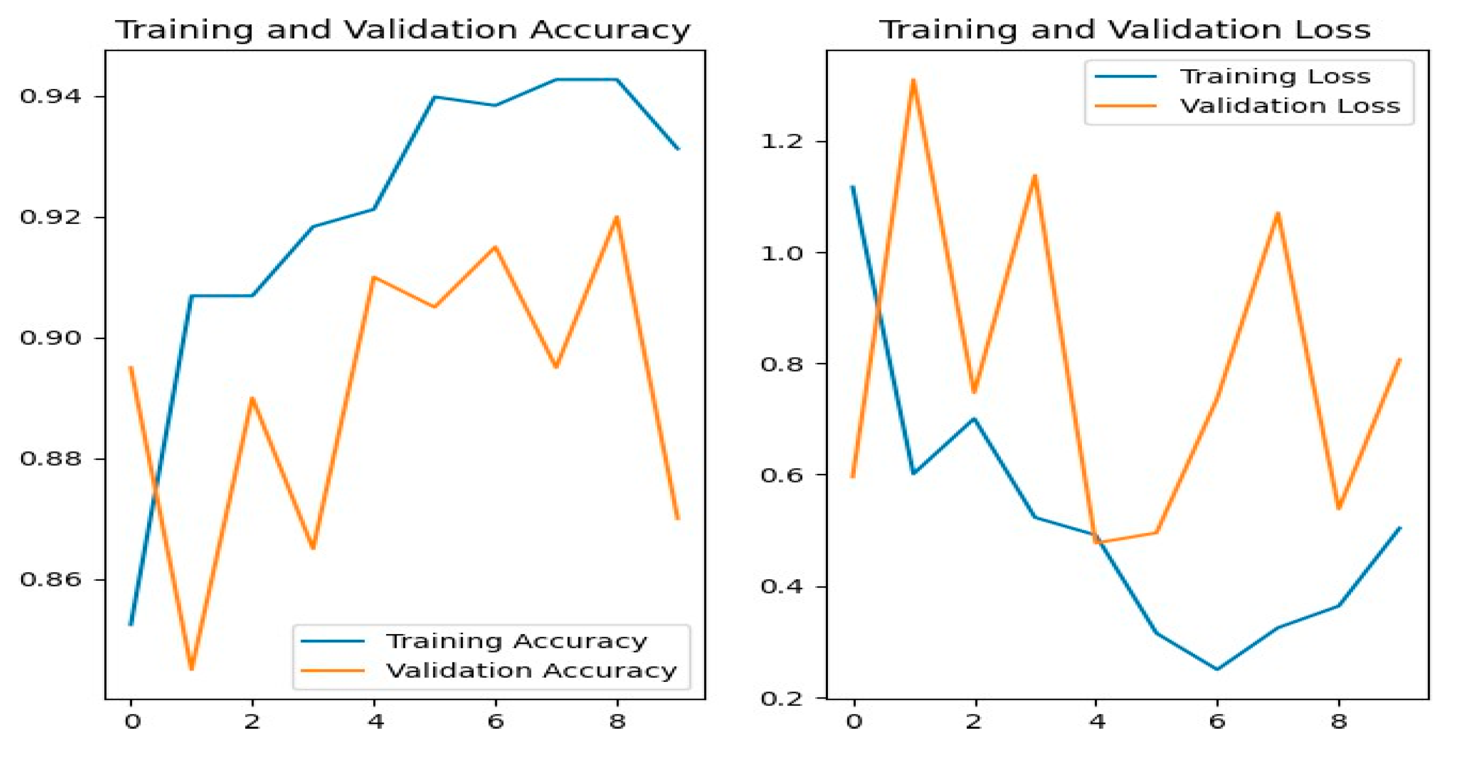
Figure 15.
MobileNetV3 Training-Validation Loss and Accuracy.
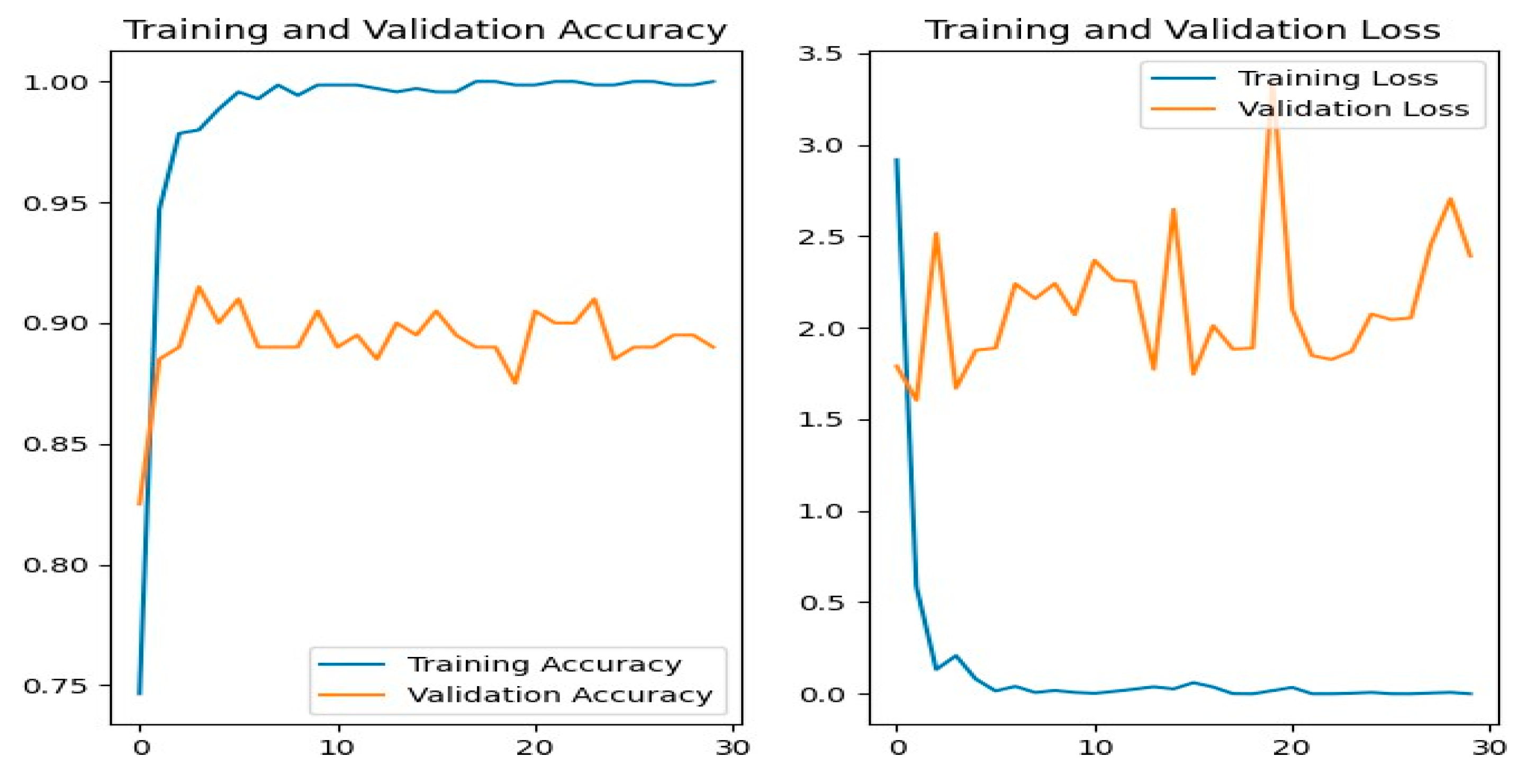
Figure 16.
DenseNet201 Training-Validation Loss and Accuracy.
Discussion
On the dataset, different methods give different results. Conversely, the result changes based on the dataset—that is, depending on whether the dataset has been changed or whether a new dataset using the same method is used. Our goal was to beat the accuracy of past study on this particular collection of diseases found in mango leaves. In our thesis work, we applied four deep learning methods to achieve our goals. In order to find a better accuracy, In our dataset, we applied five algorithms: ResNet-50, Mobile-NetV2, Vgg-19, MobileNetV3 and DenseNet-201. For these five methods, We found the precision, accuracy, and extra measures. One of the most clear things is that the algorithm’s result relies on the dataset’s features. A dataset that includes mistakes will give incorrect accuracy, and if the dataset’s traits change, the model’s estimate will also change. The best accuracy of 96.49% is achieved by ResNet- 50 out of the five methods that we used on our dataset. The creator gives this information to experts so they can work on diseases identification in mango leaves. We tried to compare our trial results with those of other studies because we also applied CNN and deep learning models. The goal of this study is to provide information about algorithm selection and adaptation from prior works to researchers who will work with utilizing deep learning models to find illnesses in mango leaf.
Limitations
While the suggested method shows high accuracy in spotting mango leaf diseases, it has some drawbacks. First, the sample is relatively small (998 pictures), which may not capture the full range of real-world situations. Environmental factors like lighting, leaf direction, and background sounds may affect model effectiveness. Additionally, the system was taught using data from limited regional locations, which may lower its generalizability to other areas or mango types. Hardware needs, such as high-configuration systems for training deep models, also pose a problem for broad use.
Future Work
Future improvements could include increasing the dataset with more varied and high-quality pictures from various areas and under different weather situations. Incorporating data enhancement methods and real-time picture capture can improve stability. A mobile tool could be made for on-field disease spotting to help farms directly. Further study can also explore lightweight models suited for low-resource devices and assess the merging of IoT and remote sensors for constant tracking of plant health.
Conclusions
In conclusion, Farmers will gain from this study in spotting leaf diseases more correctly. They can then study leaf diseases and offer cures for mango output based on the data. Our study wants to improve mango leaf disease detection through the use of CNNs with a focus on the RESNET-50 model and an accuracy of 96.49%. We also covered the classification report, the Confusion Matrix, and other graphics. The final the goal of this project is to build and improve an application for leaf disease identification that for our people, the method is easier to utilize. RESNET-50 is more accurate than other types, it was carefully picked. This shows how committed we are to using state-of-the-art tools to help mango farmers. We will continue our study to improve the efficiency of the method.
References
- Golhani, K., S. K. Balasundram, G. Vadamalai, and B. Pradhan. 2018. A review of neural networks in plant disease detection using hyperspectral data. Information Processing in Agriculture 5, 3: 354–371. [Google Scholar] [CrossRef]
- Rashed, M., and M. I. kakon. 2025. A Comparison of CNN Performance in Skin Cancer Detection. Preprints. [Google Scholar] [CrossRef]
- Arivazhagan, S., and S. V. Ligi. 2018. Mango leaf diseases identification using convolutional neural network. International Journal of Pure and Applied Mathematics 120, 6: 11067–11079. [Google Scholar]
- Singh, U. P., S. S. Chouhan, S. Jain, and S. Jain. 2019. Multilayer convolution neural network for the classification of mango leaves infected by anthracnose disease. IEEE access 7: 43721–43729. [Google Scholar] [CrossRef]
- Maheshwari, K., and A. Shrivastava. 2020. A review on mango leaf diseases identification using convolution neural network. International Journal of Scientific Research & Engineering Trends 6, 3: 1399–1403. [Google Scholar]
- Patil, R. Y., S. Gulvani, V. B. Waghmare, and I. K. Mujawar. 2022. Image based anthracnose and red-rust leaf disease detection using deep learning. TELKOMNIKA (Telecommunication Computing Electronics and Control) 20, 6: 1256–1263. [Google Scholar] [CrossRef]
- Krishnamoorthy, N., L. N. Prasad, C. P. Kumar, B. Subedi, H. B. Abraha, and V. E. Sathishkumar. 2021. Rice leaf diseases prediction using deep neural networks with transfer learning. Environmental Research 198: 111275. [Google Scholar]
- Khan, S. H., M. N. Hossain, S. Mozumder, S. Sharmin, and N. N. Moon. 2021. Rose leaf disease detection using cnn. In 2021 IEEE International Conference on Robotics, Automation, Artificial-Intelligence and Internet-of-Things (RAAICON), December; IEEE, pp. 37–41. [Google Scholar]
- Ghazi, M. M., B. Yanikoglu, and E. Aptoula. 2017. Plant identification using deep neural networks via optimization of transfer learning parameters. Neurocomputing 235: 228–235. [Google Scholar] [CrossRef]
- Moyazzoma, R., M. A. A. Hossain, M. H. Anuz, and A. Sattar. 2021. Transfer learning approach for plant leaf disease detection using CNN with pre-trained feature extraction method Mobilnetv2. In 2021 2nd International Conference on Robotics, Electrical and Signal Processing Techniques (ICREST), January; IEEE, pp. 526–529. [Google Scholar]
- Rizvee, R. A., T. H. Orpa, A. Ahnaf, M. A. Kabir, M. R. A. Rashid, M. M. Islam, and M. S. Ali. 2023. LeafNet: A proficient convolutional neural network for detecting seven prominent mango leaf diseases. Journal of Agriculture and Food Research 14: 100787. [Google Scholar] [CrossRef]
- Khan, S. H., M. N. Hossain, S. Mozumder, S. Sharmin, and N. N. Moon. 2021. Rose leaf disease detection using cnn. In 2021 IEEE International Conference on Robotics, Automation, Artificial-Intelligence and Internet-of-Things (RAAICON), December; IEEE, pp. 37–41. [Google Scholar]
- Methun, N. R., R. Yasmin, N. Begum, A. Rajbongshi, and M. E. Islam. 2021. Carrot disease recognition using deep learning approach for sustainable agriculture. International Journal of Advanced Computer Science and Applications 12, 9. [Google Scholar] [CrossRef]
- Gandhi, R., S. Nimbalkar, N. Yelamanchili, and S. Ponkshe. 2018. Plant disease detection using CNNs and GANs as an augmentative approach. In 2018 IEEE international conference on innovative research and development (ICIRD). IEEE, May, pp. 1–5. [Google Scholar]
- Salauddin, M., M. Rashed, and M. I. Kakon. 2025. Deep Learning-Based CNN Approach for Tomato Leaf Disease Detection. Preprints. [Google Scholar] [CrossRef]
- Rahman, M. S., M. Rashed, and M. I. Kakon. 2025. Deep Learning Approach for Rice Leaf Disease Detection Using CNN Models. Preprints. [Google Scholar] [CrossRef]
Disclaimer/Publisher’s Note: The statements, opinions and data contained in all publications are solely those of the individual author(s) and contributor(s) and not of MDPI and/or the editor(s). MDPI and/or the editor(s) disclaim responsibility for any injury to people or property resulting from any ideas, methods, instructions or products referred to in the content. |
© 2025 by the authors. Licensee MDPI, Basel, Switzerland. This article is an open access article distributed under the terms and conditions of the Creative Commons Attribution (CC BY) license (http://creativecommons.org/licenses/by/4.0/).
Copyright: This open access article is published under a Creative Commons CC BY 4.0 license, which permit the free download, distribution, and reuse, provided that the author and preprint are cited in any reuse.


