Submitted:
16 June 2025
Posted:
19 June 2025
You are already at the latest version
Abstract
This paper presents a Fine-grained Feature Extraction U-Net (FgFEU-Net) model to realize automatic localization and segmentation of breast cancer lesions with breast ultrasound images. In the FgFEU-Net model, we used the transfer learning method to replace the coding part of the backbone network with the VGG16 model to achieve deep and fine-grained feature extraction. The extracted low-level information is combined with the high-level knowledge of the U-Net decoding layer at the same layer and converted into high-resolution information to pinpoint lesions precisely. Finally, the high-resolution information is transformed into a high-resolution image through the final convolutional layer. In addition, the combo loss is adopted to deal with the imbalance between organ input images and their output images. The proposed model was tested and predicted in the BUS2018 (Breast Ultrasound Images 2018) dataset, and the proposed evaluation metric of accuracy, precision, and sensitivity reached 99.03%, 96.83%, and 99.35%, respectively.
Keywords:
breast tumor
; deep learning
; transfer learning
; combo loss
; semantic segmentation
1. Introduction
Biomedical image segmentation is essential in many medical applications [1,2]. Although segmentation methods based on CNN (convolutional neural network) can achieve accuracy, these methods usually rely on supervised training with large labeled datasets [3,4]. Annotating biomedical images requires a lot of expertise and time and is not feasible on a large scale. To solve the problem of labeling data, researchers usually use manual preprocessing, manual adjustment of the framework structure, and data augmentation [5]. However, these techniques involve complex engineering work and are often targeted to specific datasets.
According to statistics from the International Agency for Research on Cancer (IARC) under the WHO, 8.2 million people died of cancer in 2012, which is expected to rise to 27 million in 2030. Breast cancer is one of the most severe diseases of women [6,7]. Breast cancer diagnosis is usually performed by imaging systems or procedures, such as mammography, MRI, ultrasound images, and thermal imaging [8,9,10,11]. Medical image science research for cancer screening has been conducted for over 40 years. However, in clinical applications, live detection based on case images is undoubtedly the standard for detecting breast cancer. It is also essential for doctors to take the best treatment measures when accurately classifying pathological images.
There are usually two methods of detecting breast tumors. One is an artificial feature extraction-based image classification method, and the other is a deep learning-based pathological image classification method [12,13]. Traditional artificial feature-based breast cancer pathological classification methods mainly use artificial extraction features and support vector machines, random forests, nearest neighbor algorithms, and other classifiers to complete the classification based on these features [14,15,16]. In addition, since medical images involve patient privacy and medical ethics issues, the samples available for deep learning (DL) model training on breast cancer pathology images are minimal, which will seriously affect the model prediction accuracy and precision [17,18]. Based on previous research, we propose an enhanced transfer learning-based method for breast tumor segmentation and perform validation experiments on the Breast Ultrasound 2018 (BUS2018) [19] dataset. Firstly, the normalization [20] method is used for data preprocessing because the image sizes in the dataset are inconsistent. Secondly, data enhancement techniques such as flipping, translation, and denoising are used to process the graphics to expand the amount of trainable data [21,22]. Finally, the current popular U-Net medical image segmentation model is adopted as the basic model [23], and an improved model is constructed with VGG16 [24,25]. ReLU is adopted as the activation function [26]. In the DL model, binary cross entropy loss and dice coefficient loss are often used [27]. The advantage of this method is that in small sample datasets, the model can improve the accuracy of tumor segmentation without reducing the accuracy.
For medical image processing and analysis tasks, the network model needs to consider the image’s high-level semantic information and low-level features [28,29]. Traditional segmentation methods often used include RF (Random Forest) algorithm, kNN (K-Nearest Neighbor) algorithm, SVM (Support Vector Machine), and DL approaches, including CNN, LSTM, Bi-LSTM, ResNet, DenseNet, and VGGNet [30,31,32,33].
Edge detection, template matching techniques, and statistical models were employed in early medical image segmentation tasks. Zhao et al. [34] proposed an edge detection-based algorithm lung CT image segmentation technique. Lalonde et al. [35] used a template-matching method based on Huffman sentence distance for tumor image segmentation. Chen et al. [36] proposed a template matching method to achieve tumor image segmentation in brain CT. Tsai et al. [37] adapted a shape-based method 2D and 3D segmentation method for prostate MRI images. Li et al. [38] adopted an active profile model to segment liver tumors from abdominal CT images. In contrast, Li et al. [39] proposed a BBDS (Biomedical Body Data Segmentation) framework by CLS (Combining Level Sets) and SVM.
We have benefited from a literature review of research on medical image segmentation, some of which are impressive. Inspired by [40], we adopt dice loss [41] and Binary Cross-entropy loss (BCE) [42,43] to compose the combo loss function of the proposed enhanced model. Compared with the model training prediction in the case of Tversky (TC), BCE, and dice loss, we try to find the best model performance for breast tumor segmentation. Constructing an improved CNN model and selecting an appropriate loss function to realize breast tumor semantic segmentation is challenging when the number of sample categories is unevenly distributed.
The main contributions of this paper are as follows:
- (1)
- Based on the transfer learning (TL) method, the FgFEU-Net model is proposed for breast tumor segmentation. The model adopts U-Net model as the backbone network, Vgg16 as the pre-training model for fine-grained feature extraction, and adopts combined loss as a loss function.
- (2)
- To solve the imbalance between input and output in organ images, the combination loss is employed in the experiments. The performance of the model with TC loss, dice coefficient, and binary cross loss are compared with lots of experiments, respectively.
- (3)
- The model performance is compared with SVM, CNN, VGG16, VGG19, and U-Net in the same dataset. Experimental results indicate that the proposed model obtained the best segmentation performance.
The rest of this paper is organized as follows. Section 2 is related work. Section 3 is the methodology, including the proposed method, loss function, and evaluation metrics. Section 4 presents experiments and analysis, including experimental dataset description, experimental procedure, experiment result, and discussion. Section 5 presents the conclusion.
2. Related Work
Since the feature learning CNN is used to be insensitive to image noise, blur, contrast, and so on, CNN models exhibit excellent performance in medical images [44]. In 2015, Ronneberger et al. [23] proposed a U-shaped semantic segmentation network for medical image processing, which attracted the attention of researchers. It is a fully symmetrical U-net structure based on image encoding and decoding and adopts the skip-connection mechanism [45,46]. In 2019, Isensee et al. [47] proposed an adaptive medical image segmentation model no-new-Net (nnU-Net). The basic model of this method is U-Net.
In the numerous literature, in addition to establishing DL models, researchers mainly optimize the model from data preprocessing, loss function selection, supervision strategy of the training process, and so on. Seyed et al. [48] used the Tversky Loss (TC) function as a loss function for image segmentation with 3D fully connected CNNs. Yeung et al. [49] use unified focal loss as the loss function to solve the imbalance problem of the distribution of the number of medical images sample categories. In this method, the author adopts the generalized dice and Cross-Entropy (CE) loss to construct the Unified Focal loss function. CE loss is a typical function widely used in classification tasks and applied to the currently popular U-Net model [50]. In contrast, the attention-based U-Net method proposed by Schlemper et al. [51] and the V-Net model by Milletari et al. [52] applied the dice coefficient as the loss function. In image segmentation tasks, loss functions are roughly divided into assignment-based, region-based, and boundary-based [53].
In recent years, more and more classification tasks have used the combined loss as the loss function and achieved perfect results. Taghanaki et al. [40] employed dice and cross-entropy loss to construct a loss function for the segmentation task. Although these loss functions perform well in specific medical image segmentation tasks, they are not general and are primarily used based on particular models and large datasets to perform well. Galli et al. [54] proposed a pipelined tracer-aware approach for breast tumor detection. This method uses the three-time-points (3TP) processing process to achieve feature extraction and detection of breast tumors. However, this method is implemented based on the DCE-MRI method, which requires continuous sampling of images and consumes a lot of computation.
In addition, Yang et al. [55] proposed the CTG-Net cross-task network framework in breast tumor segmentation, Zovathiet al. [56] adopted the region labeling-based breast lesion segmentation method, and Fu et al. [57] proposed the automatic breast cancer segmentation framework based on attention mechanism. The AlexSegNet network proposed by Singha et al. [58] was used for breast tumor segmentation. According to the latest DL trend of nuclear segmentation in histopathological images by Basu et al. [59], from 2017 to 2021, medical image segmentation has developed from the original CNN to the current U-Net model and corresponding variant models, and the segmentation accuracy has been significantly improved. These research pieces of literature guide our research work.
3. Methodology
In this section, we propose a DL-based model on tumor segmentation in breast ultrasound images based on the theory of TL and present several loss functions based on this model. In addition, we briefly introduce the model evaluation metrics.
3.1. Proposed Approach
Basic U-Net Model. The U-shaped Network (U-Net) was proposed by Ronneberger et al. [23] at the MICCAI conference in 2015. It is a breakthrough in DL in medical image segmentation tasks. U-Net model is developed based on FCN, mainly including an encoder, BN (Bottleneck module), skip-connection, decoder, and other parts. The structure of our expected U-Net model for the breast cancer tumor segmentation is shown in Figure 1.
Pre-trained Model. Based on the DL model, the VGG16 trained on the ImageNet. It is adopted in object recognition, object classification, and other tasks due to features and low-level detail extraction characteristics. In the VGG16 model, the pre-trained weights of the VGG16 network are derived from the large image dataset ImageNet. The ImageNet image dataset contains 3.2 million annotated images in 5247 categories, characterized by large scale, deep hierarchical density, diversity, and complexity. Therefore, the pre-trained weights obtained in this dataset have better generalization and robustness. Applying pre-trained weights obtained in extensive data sets to medical image processing with small data samples can achieve better results and improve the efficiency of feature extraction and prediction accuracy using the concept of TL.
Overall Architecture. To meet the small sample segmentation task, we employed the TL method to fuse VGG16 and U-Net networks with an FgFEU-Net model to achieve the mission of breast tumor segmentation. The proposed network structure is shown in Figure 2. The model is mainly constructed by five parts, such as input layer, encoding layer, decoding layer, final convolution layer (Final-conv2D), and output layer.
The input layer is the input of the original image, the size is normalized to a dimension of 256 × 256 × 3, and the output layer is the segmentation mask of the predicted breast cancer lesion area. The encoding layer consists of the first ten layers of the VGG16 network. These ten layers are divided into four pairs of stacks, each subjected to 2 or 3 convolution operations. A dropout layer is introduced in the convolution operation to prevent model training from overfitting. The convolution kernel size in the stacked layer is 3 × 3, the encoding layer is output through the maxpool layer, and the window size of the maxpool layer is 2×2. As the number of network layers increases, the number of convolution kernel channels doubles after each pooling operation until it equals 512. Because the sample data of the experimental dataset is small, the first ten layers of parameters of the VGG16 pre-training model are used to initialize the parameters of the encoding layer convolution kernel through the TL method. It can speed up the model convergence while enhancing the model generalization ability. Due to the deepening of the depth of the network layer, the representation of the input by the encoding layer is more and more abstract, higher-dimensional features are extracted at the same time, and the feature expression ability of the image is gradually enhanced. After the coding layer processing, the image scale is reduced to 16 × 16.
The decoding layer adopts the U-Net network structure, which consists of four layers linked to the upsampling operation. Each layer also performs 2-3 different convolution operations. The convolution kernel size is 3 × 3, and the dropout layer is set between the convolution layers. Contrary to the encoding layer, convolution kernel channels gradually decrease as the decoding layer goes deeper. In the up-sampling operation, the traditional fully connected convolutional neural (FC) maps the image layer by layer and only up-samples the final mapping result to obtain an image whose size is the same as the input image, ignoring the intermediate mapping layer in the process. The output information has a particular symbolic ability for the image. The decoding layer utilizes the idea of the residual network. It connects the information of the intermediate mapping layer with the corresponding decoding layer by constructing a copy channel so that the gradient context information can be propagated to the higher resolution layer to combine the deep abstract features with the corresponding decoding layer. The shallow features are combined to locate the gray-level category image information.
The final convolution layer (Final-Conv) performs two convolution operations, the convolution kernel size is 3 × 3, 1 × 1, and the number of convolution kernels is 3. After two convolution operations, the image size is restored to the exact dimensions of the input image.
In the FgFEU-Net model, image encoding is the process of down-sampling. The encoding layer comprises four convolution operations and pooling operations stacked, and the convolution kernel and maximum pooling window sizes are 3×3 and 2×2, respectively. In the first layer, the convolution kernels is 64, then increases layer by layer, and the number of convolution kernels in the fourth layer is 512. Similarly, the process of image decoding is also the process of up-sampling. The decoding layer also contains four layers. Each decoding layer comprises the convolution kernel and max pooling layers, and an up-sampling operation links each stack. The convolution kernel size of each layer is 3 × 3, and the maxpool window size is 2 × 2. The number of convolution kernels gradually decreases from bottom to top, and the number of convolution kernels in the fourth layer is 64. The fourth layer of the decoding layer is linked with the final convolutional layer. After the final convolutional layer has undergone two convolutions, the segmentation mask of the breast cancer tumor is output through the Sigmoid classification function.
In our proposed FgFEU-Net model, the features of high-order and low-order images are extracted hierarchically by constructing replication channels, thus ensuring that the final output image contains the contextual information of the original image. In the down-sampling part, we adopt four convolution operations. The features of breast cancer tumor lesions in the sample image are extracted layer by layer by including convolution kernels of different sizes in each layer through the four-layer deconvolution operation in the up-sampling part. The information of the intermediate mapping layer is connected with the corresponding decoding layer information by constructing a replication channel. In this process, the high-resolution extraction of layer-by-layer low-level information is realized to accurately locate the location of tumor lesions, realize the semantic segmentation of tumor lesions, and help clinicians identify breast cancer tumor lesions and diagnose the disease.
3.2. Loss Function
Binary Cross-entropy Loss. Cross-entropy (CE) [42,60] measures the difference between two probability distributions for a given random variable or set of events. Since the cross-entropy loss is pixel-level segmentation, excellent results can be obtained in image segmentation tasks. BCE Loss is the binary classification cross-entropy loss. Since the breast tumor segmentation task is a classification task of background and lesion mask, it is a binary classification task. Hence, BCE loss is very suitable for this task. The definition of BCE Loss is shown in equation (1).
Here, y is the actual value of the sample, andis the predicted value.
Dice Coefficient Loss. Dice coefficients are often employed to measure the similarity of two samples in the DL model. The range of dice coefficients is [0,1], the larger the value, the closer the segmentation effect is to the actual value. In 2016, Carole et al. [27] used Dice loss as an essential indicator for model evaluation. Since then, the Dice Loss function has been familiar to researchers. The definitions of Dice coefficient and Dice Loss are shown in equations (2) and (3). Here, one is added in the numerator and denominator to ensure that the function is not undefined in edge-case scenarios such as when y==0. From equation (3), then the dice loss is region-related loss. It means that a pixel loss and gradient value are related to the label and predicted value of that point, and the label and expected value of other problems, which is different from CE loss and BCE.
Tversky Coefficient Loss. Seyed et al. [44] proposed the Tversky Loss function in CVPR 2018 based on the Tversky coefficient (TC). The TC mainly describes the similarity between the two features. TC is an extension of the dice coefficient, which uses α and β penalty coefficients to increase the weight of false positives (FP) and false negatives (FN). TC is defined as equation (4).
Here, when α = β = 0.5, it is regarded as a regular dice coefficient. Equation (5) is the definition of TC loss.
Here, 1 is added to the numerator and denominator to prevent the denominator from having a 0 value.
Combo Loss. Since BCE Loss performs well in two-class DL models, it can solve the gradient descent problem of model learning, especially in the learning rate gradient descent of small sample dataset training. On the other hand, because dice Loss can solve the problem of model overfitting well, it is widely used in medical image segmentation tasks, showing excellent performance. However, because the error curve in the model training is very confusing using dice Loss, it is difficult to observe the model convergence information, which is generally replaced by checking the error on the validation set. Therefore, combining the advantages of BCE and dice loss and maximizing the elimination of the interference caused by unfavorable factors, we use BCE and dice loss to form a combined loss function. The definition of combo loss is shown in equation (6).
Finally, the calculation of the combo loss is shown in equation (7).
Here, y is the actual value of the sample, and p ̂ is the predicted value of the sample predicted by the model.
3.3. Evaluation Metrics
Dice Similarity Coefficient. To evaluate the performance of the model and the effect of image segmentation, and compare it with the prediction effect of other loss functions, we adopt the DSC evaluation index [60,61,62]. The DSC is calculated by equation (8).
where the symbol P and R are predictive and actual labels, respectively. TP, FP, and FN represent true positive, false positive, and false negative rates. In addition, we also calculated the sensitivity and precision metrics of semantic segmentation, and the calculation formulas are shown in equations (9) and (10).
MIoU. MIoU (Mean Intersection over Union) is a standard metric for semantic segmentation. MIoU is obtained by calculating the average of the intersection and union ratio of the two sets of actual and predicted values. Compared with the IoU metric, MIoU can better demonstrate the segmentation performance of the model. In the semantic segmentation task, these two sets are the ground truth denoted as G, and the predicted value (Predicted Segmentation) denoted as P. Assuming that i represents the actual value, j represents the expected value. Pij represents the probability of predicting i as j, then MIoU is calculated by equation (11), which is equivalent to equation (12).
4. Experiments and Analysis
Based on the proposed model, loss function, and evaluation metrics described in section 3, we conducted detailed experiments, which will be described in this part, including dataset description, experimental procedures, experiment environment, and results. Finally, we discuss the experiment result.
4.1. Dataset Description
All images from the BUS2018[19] dataset were collected at baseline, including breast ultrasound images from women aged 25 to 75. These images were obtained in 2018. In this study, we use BUS2018 an experimental dataset which includes 874 benign tumor images, 266 normal images, and 420 malignant tumor images, both real and mask images. The average image size is 500×500 pixels, and the images are in PNG format. Due to the varying size of the sample images, we process all images size to 256 × 256 pixels. Since the mask feature value of normal sample images is zero, we only use benign and malignant tumor images and their mask for model training, a total of 1294 images. Since the number of samples is minimal, we divide the new dataset into a training and test dataset in a ratio of 8:2.
4.2. Experimental Procedures
The purpose of breast tumor image segmentation is to quickly and accurately identify the location of tumor lesions in breast ultrasound images and automatically generate tumor masks, providing an essential basis for doctors to diagnose diseases. Therefore, in our experiment, an ultrasound image of breast cancer (an ultrasound image with lesions) is input, the location of the lesion can be accurately predicted by the model, and the corresponding mask is generated. At the same time, calculate the DSC, MIoU, and precision values. The experimental procedure mainly includes the following four steps.
Data preprocessing. Due to the different sizes of the sample images in the BUS2018 dataset, we need to normalize the images first. In the data preprocessing process, invalid ultrasonic images were eliminated, and the size of all images was processed as 256 × 256.
Model parameter settings. As described in Section 3, in the encoding and decoding parts of the proposed model, we set the convolution kernel size to 3 × 3 and the pooling window size to 2 × 2, and extracted breast tumor ultrasound image lesions feature through the VGG16 model. The deep-level fine-grained information is merged with the up-sampling layer of the decoding part at the same layer and restored to high-resolution lesion information, which provides high-level information for the precise localization of lesions in the final convolutional layer. Considering the tiny number of samples, we set the batch size to 8, the training epoch to 100, and ReLU as an activation function. The initial learning rate is 0.00001, the learning rate is specified in the range of [0.00001, 1), and the early-stopping mechanism is used to dynamically adjust the learning rate of model training. The dropout used in the coding part is 0.07, which retains the deep features of the lesions, and the dropout set in the decoding layer is 0.1, which contains the high-level information of the image, which provides a guarantee for the improvement of fine-grained features of the lesions and high-level information. Adam is used as the optimizer. The convolution kernel size in the final convolution layer is 3 × 3, and 1 × 1, respectively. After two convolutions, the Sigmoid classification function separates the lesion area from the background image, and the output breast tumor segmentation corresponds to the mask images.
Model training and testing. First, the TC loss is used for the loss function, and by setting six groups, different thresholds are used to train and test the model. We attempt to find the best combination of penalty coefficients through the model performance change curve to prepare for model optimization. Then, through the test dataset for model testing, check the prediction performance and evaluation indicators. In addition, we also used BCE Loss, dice loss, and combo loss to train the model, and compared the training results under different loss functions. We use the early-stopping mechanism to monitor the validation loss to avoid overfitting and try to get the best model performance during the training process.
Model prediction and evaluation. To evaluate the impact of different loss functions on model prediction results, we trained and tested the model under different loss functions in the same data set, and loss rate, accuracy rate, precision, and IoU indicators, and sampled some of the prediction results with other model prediction results are compared. The evaluation indicators such as DSC, MIoU, and PPV mask image predicted by the model are displayed.
4.3. Experimental Environment
The experiments use benign and malignant tumors and their corresponding mask images for model training and testing. After removing some sample images without mask images, the final dataset size for model training and testing is 1294, including 874 benign tumors and their mask images and 420 malignant tumors and their mask images. Since the sample data is minimal, we randomly select 80% of the images for model training and 20% for testing. In addition, we normalized the images before the model training and uniformly processed the images into a pixel size of 256 × 256 due to the different image sizes.
The experimental computer is a graphics workstation equipped with an Intel Core I7, 32G memory, and a 2T hard disk, and it can access the Internet. In addition, it is equipped with an Nvidia GeForce RTX 3060Ti graphics card. The experimental software environment uses the Windows 10 operating system with an installed scientific computing library and the Python programming language for data processing, algorithm implementation, and model construction.
4.4. Experiment Result
In the TC loss function, the effect of different thresholds (e.g., α, β) on the model training results is shown in Figure 2 shows the change curve of the loss rate and the accuracy rate during the training process. Figure 4 shows the variation curve of DSC and loss rate for model training under different thresholds. Figure 5 shows model performance curves at different thresholds. In Figure 5, we mainly examine the MIoU, Sensitivity, and PPV performance metrics of the model training process. Table 1 shows the loss and accuracy metrics of different loss functions in model training. Figure 6 shows the results of model predictions at different thresholds. Such as Figure 7, Figure 8 and Figure 9 show the performance curves of models trained with BCE loss, Dice loss, and Combo loss, respectively. Figure 10 shows the prediction results of the models trained with different loss functions. Table 2 shows the evaluation indicators of DSC, Precision, Sensitivity, and MIoU predicted by different loss function models.
In addition, we compared the proposed method with commonly used tumor lesion segmentation methods, and the experimental results are shown in Table 3 compares the proposed method with the basic CNN, VGG16, VGG19, and their enhanced models. The experimental results reveal that the proposed method performs more excellent than the traditional model segmentation. Also, in the proposed method, the FgFEU-Net model performs better segmentation than the base U-Net model. The proposed FgFEU-Net model has a lower loss rate and better accuracy in both the model training and testing phases. In all model tests, the F1 value of the FgFEU-Net model reached 0.9815, and the ROC value reached 0.9906, which is the best among all models. Therefore, experiments show that the FgFEU-Net model has excellent segmentation performance in tumor detection.
Figure 3.
Accuracy and loss rate curve of model training under different penalty coefficients by TC loss function (In where, (a) α=0.1, β=0.9, (b) α=0.2, β=0.8, (c) α=0.3, β=0.7, (d) α=0.5, β=0.5, (e) α=0.5, β=0.5, (f) α=0.70, β=0.75.).
Figure 3.
Accuracy and loss rate curve of model training under different penalty coefficients by TC loss function (In where, (a) α=0.1, β=0.9, (b) α=0.2, β=0.8, (c) α=0.3, β=0.7, (d) α=0.5, β=0.5, (e) α=0.5, β=0.5, (f) α=0.70, β=0.75.).
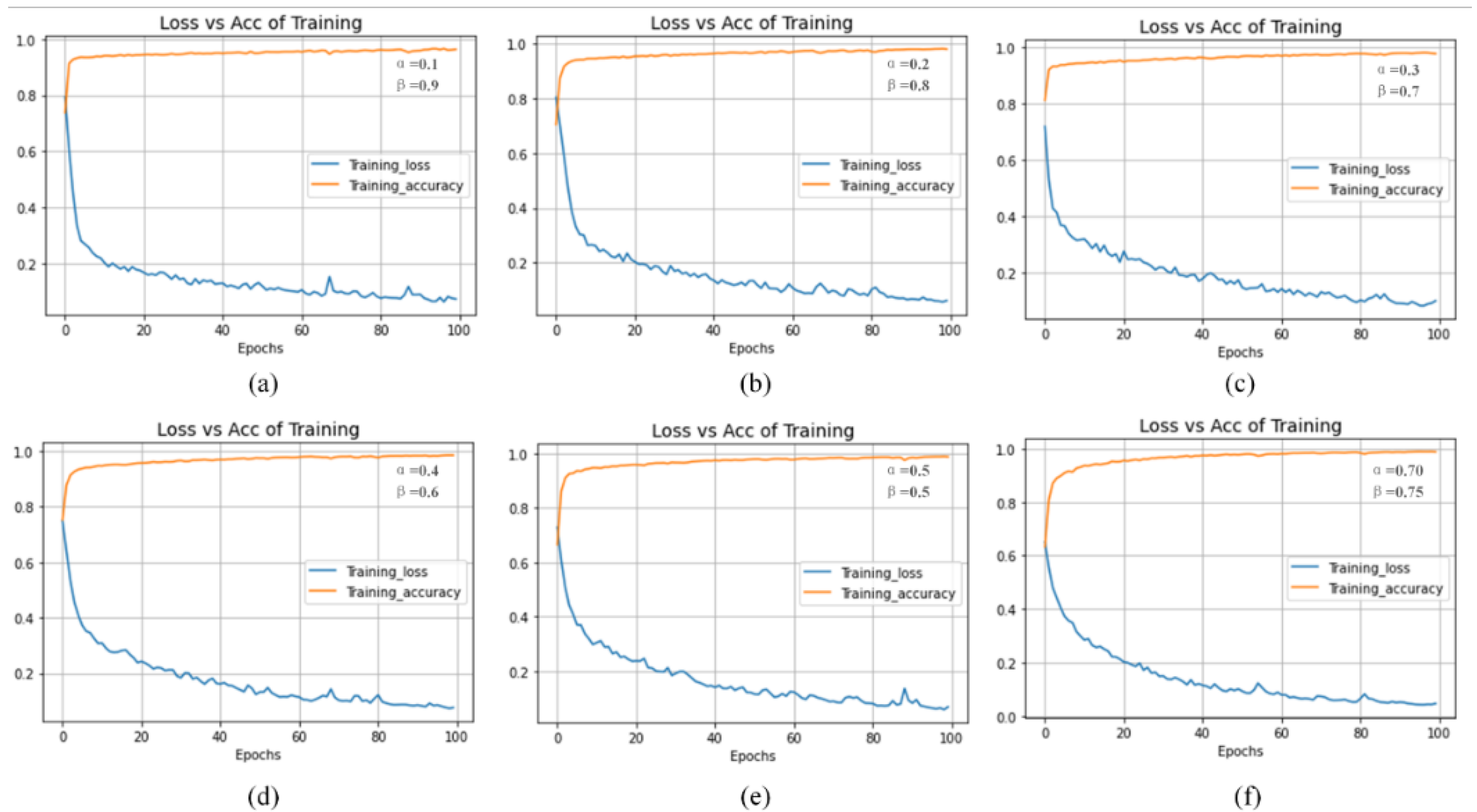
Figure 4.
Dice coefficient (DSC) and loss rate curve of model training under different penalty coefficients by TC loss function (In where, (a) α=0.1, β=0.9, (b) α=0.2, β=0.8, (c) α=0.3, β=0.7, (d) α=0.5, β=0.5, (e) α=0.5, β=0.5, (f) α=0.70, β=0.75.).
Figure 4.
Dice coefficient (DSC) and loss rate curve of model training under different penalty coefficients by TC loss function (In where, (a) α=0.1, β=0.9, (b) α=0.2, β=0.8, (c) α=0.3, β=0.7, (d) α=0.5, β=0.5, (e) α=0.5, β=0.5, (f) α=0.70, β=0.75.).
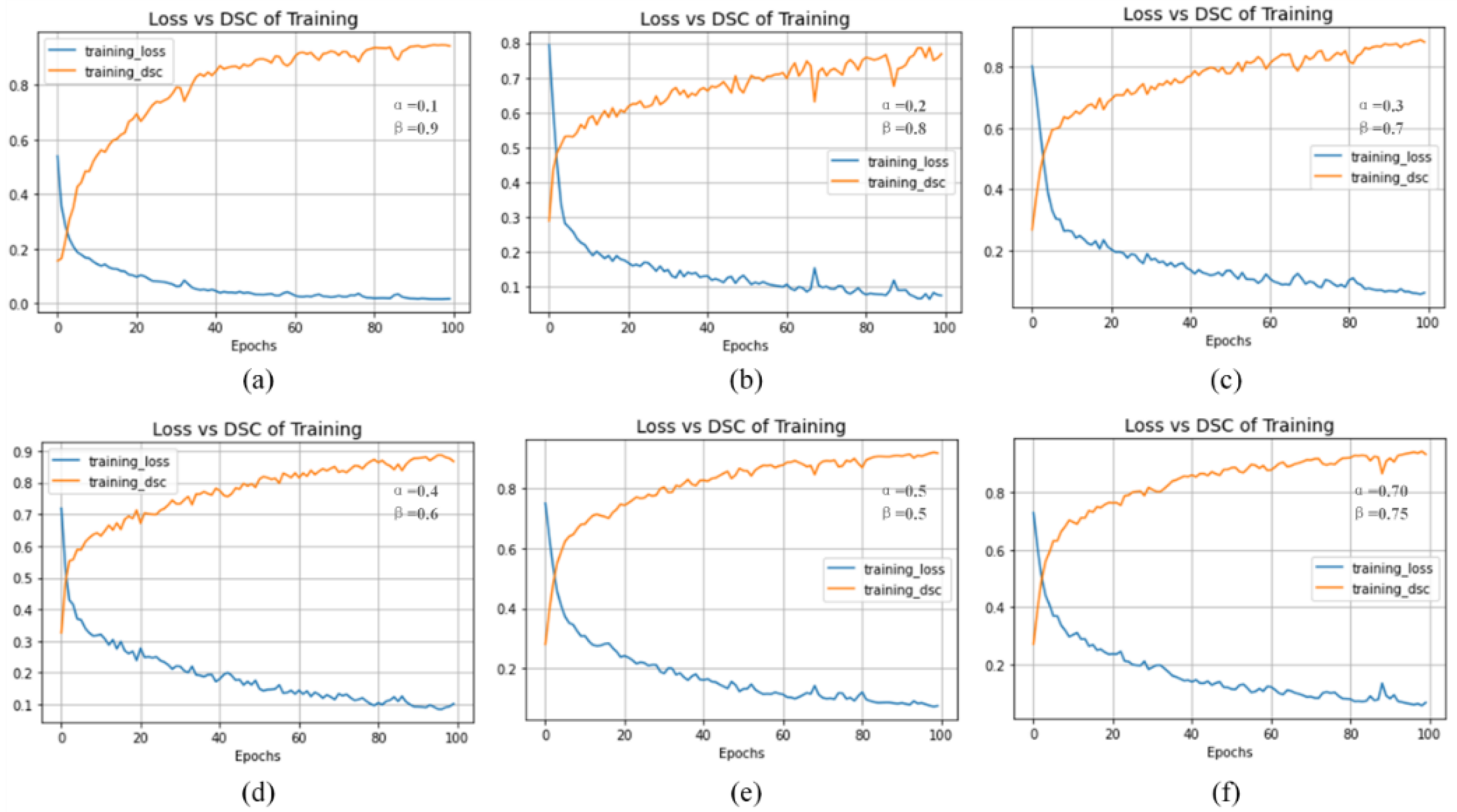
Figure 5.
Performance of model training with different penalty coefficients using TC loss function (In where, (a) α=0.1, β=0.9, (b) α=0.2, β=0.8, (c) α=0.3, β=0.7, (d) α=0.5, β=0.5, (e) α=0.5, β=0.5, (f) α=0.70, β=0.75.).
Figure 5.
Performance of model training with different penalty coefficients using TC loss function (In where, (a) α=0.1, β=0.9, (b) α=0.2, β=0.8, (c) α=0.3, β=0.7, (d) α=0.5, β=0.5, (e) α=0.5, β=0.5, (f) α=0.70, β=0.75.).
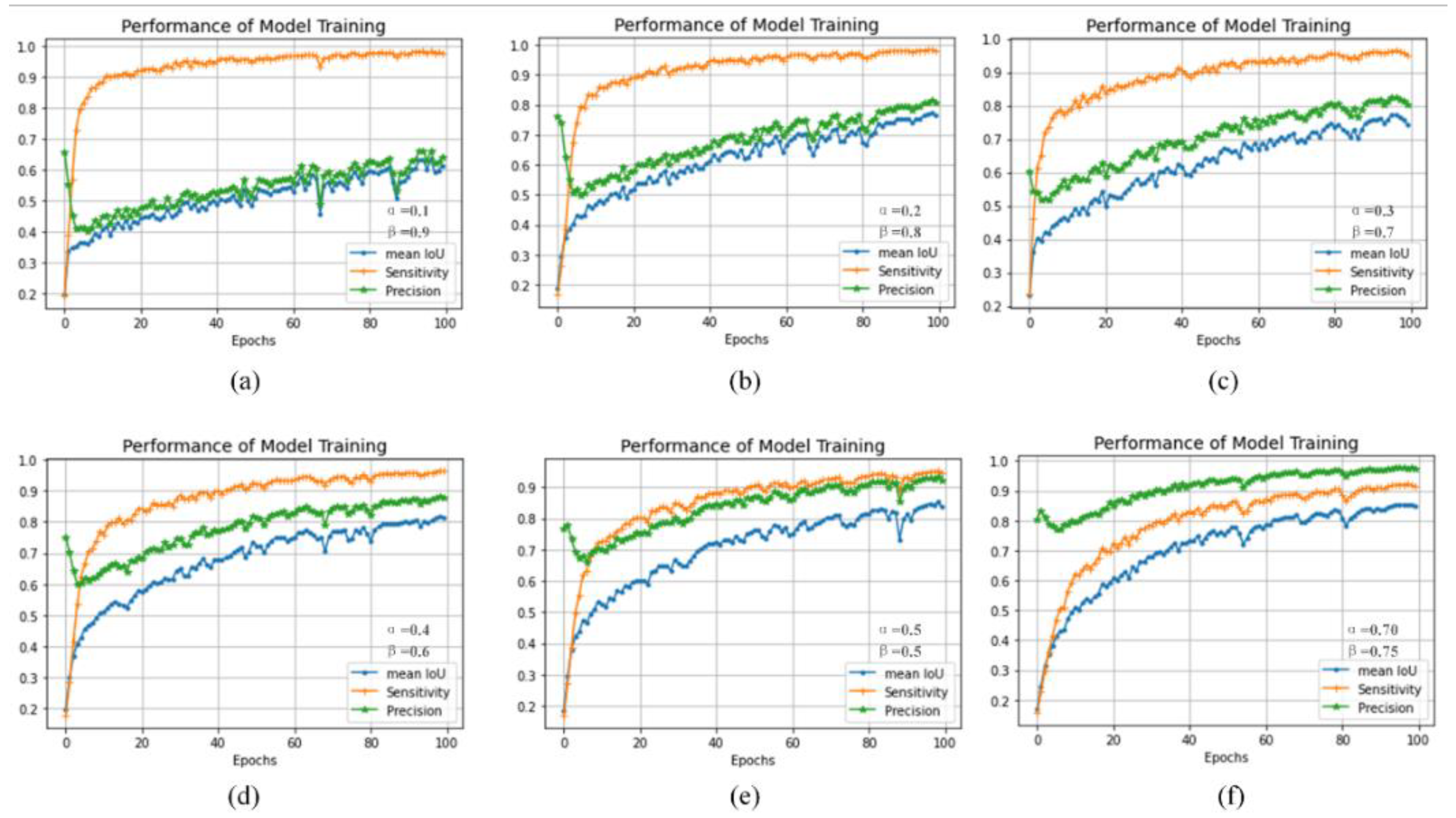
Figure 6.
Effect and evaluation metric of model prediction under different penalty coefficients with TC loss function (In where, (a) α=0.1, β=0.9, (b) α=0.2, β=0.8, (c) α=0.3, β=0.7, (d) α=0.5, β=0.5, (e) α=0.5, β=0.5, (f) α=0.70, β=0.75.).
Figure 6.
Effect and evaluation metric of model prediction under different penalty coefficients with TC loss function (In where, (a) α=0.1, β=0.9, (b) α=0.2, β=0.8, (c) α=0.3, β=0.7, (d) α=0.5, β=0.5, (e) α=0.5, β=0.5, (f) α=0.70, β=0.75.).
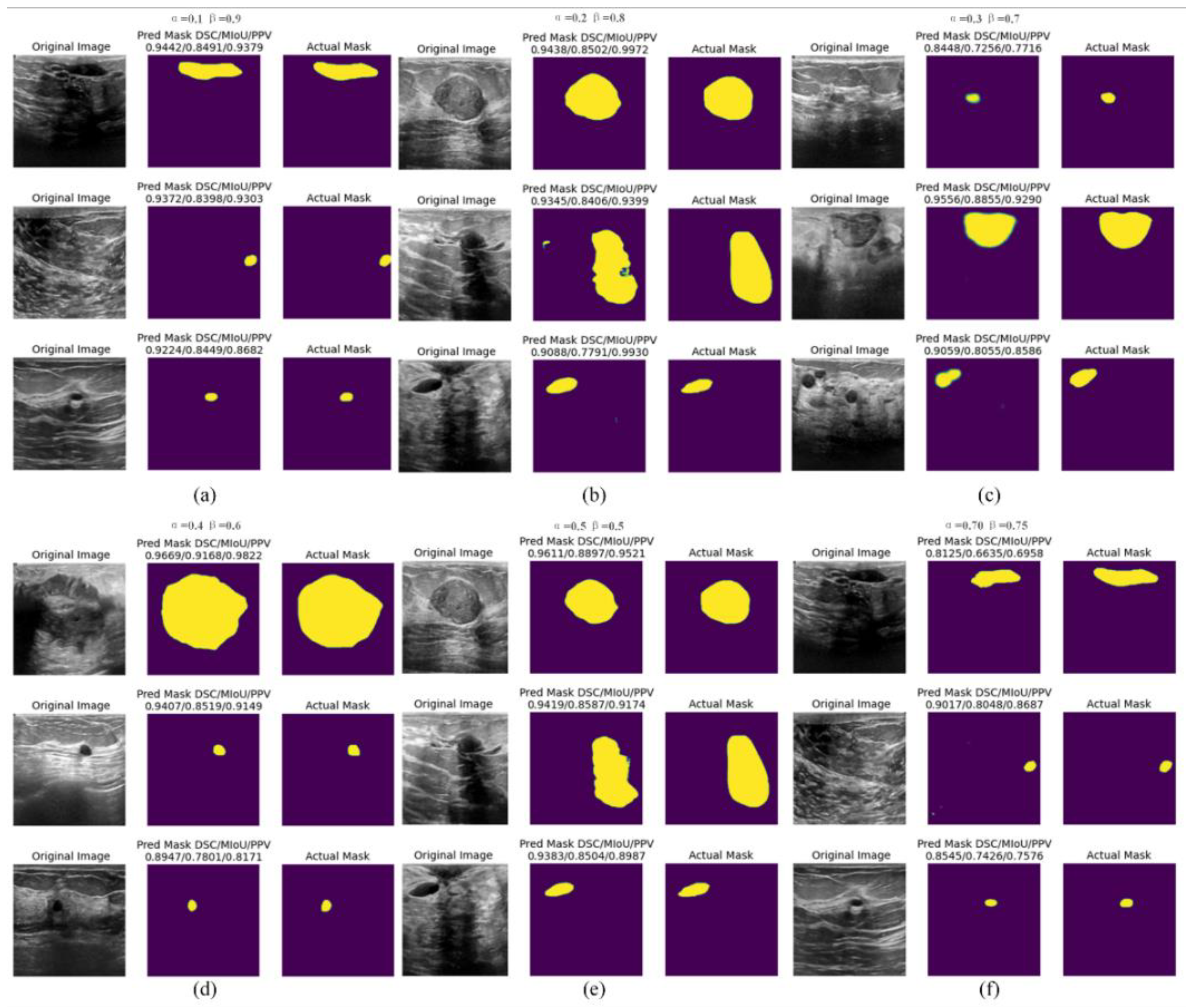
Figure 7.
The model training curve under the BCE loss function ((a) presents the loss rate and accuracy curve, (b) represents the loss rate and DSC curve, (c) illustrates the model training performance evaluation curve, including MIoU, Sensitivity, and Precision metrics.).
Figure 7.
The model training curve under the BCE loss function ((a) presents the loss rate and accuracy curve, (b) represents the loss rate and DSC curve, (c) illustrates the model training performance evaluation curve, including MIoU, Sensitivity, and Precision metrics.).
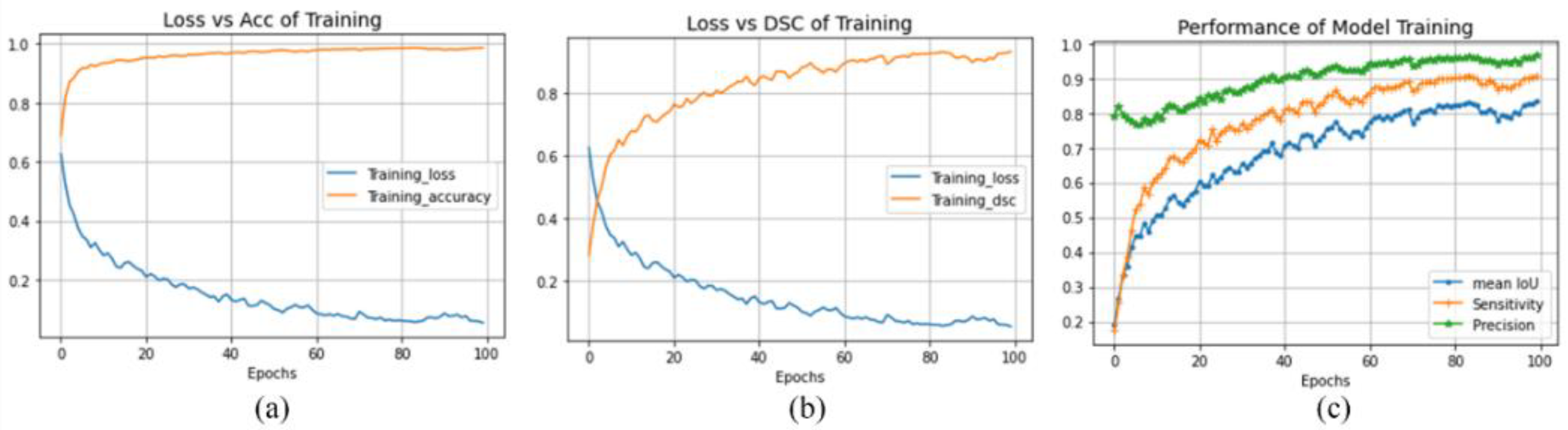
Figure 8.
The model training curve under the Dice loss function ((a) presents the loss rate and accuracy curve, (b) represents the loss rate and DSC curve, (c) represents the model training performance evaluation curve, including MIoU, Sensitivity, and Precision metrics.).
Figure 8.
The model training curve under the Dice loss function ((a) presents the loss rate and accuracy curve, (b) represents the loss rate and DSC curve, (c) represents the model training performance evaluation curve, including MIoU, Sensitivity, and Precision metrics.).
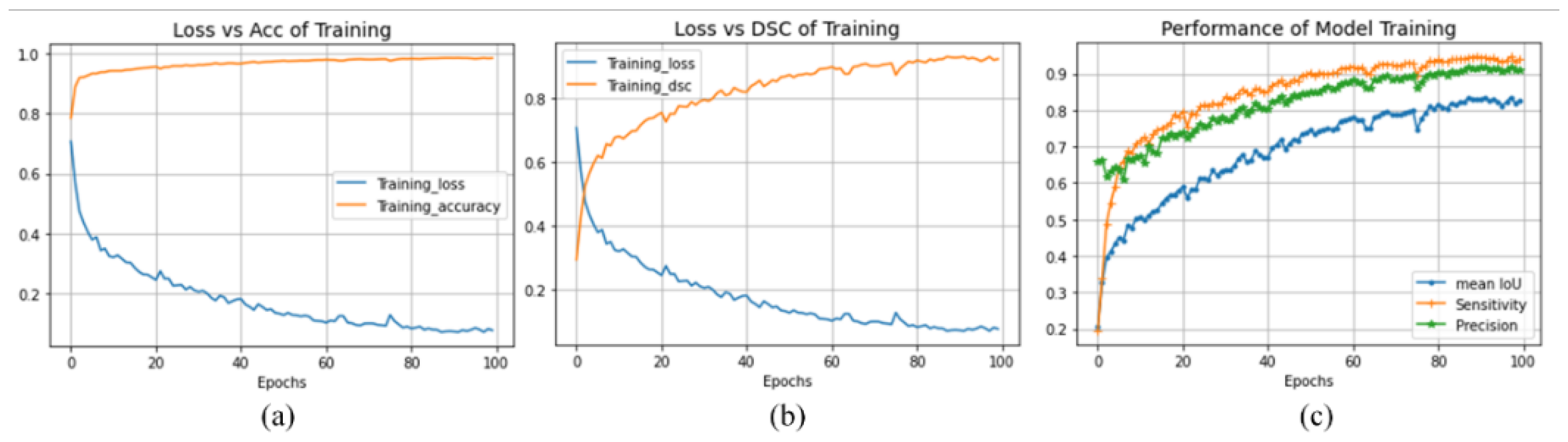
Figure 9.
The model training curve under the combo loss function ((a) presents the loss rate and accuracy curve, (b) represents the loss rate and DSC curve, (c) represents the model training performance evaluation curve, including MIoU, sensitivity, and precision metrics.).
Figure 9.
The model training curve under the combo loss function ((a) presents the loss rate and accuracy curve, (b) represents the loss rate and DSC curve, (c) represents the model training performance evaluation curve, including MIoU, sensitivity, and precision metrics.).
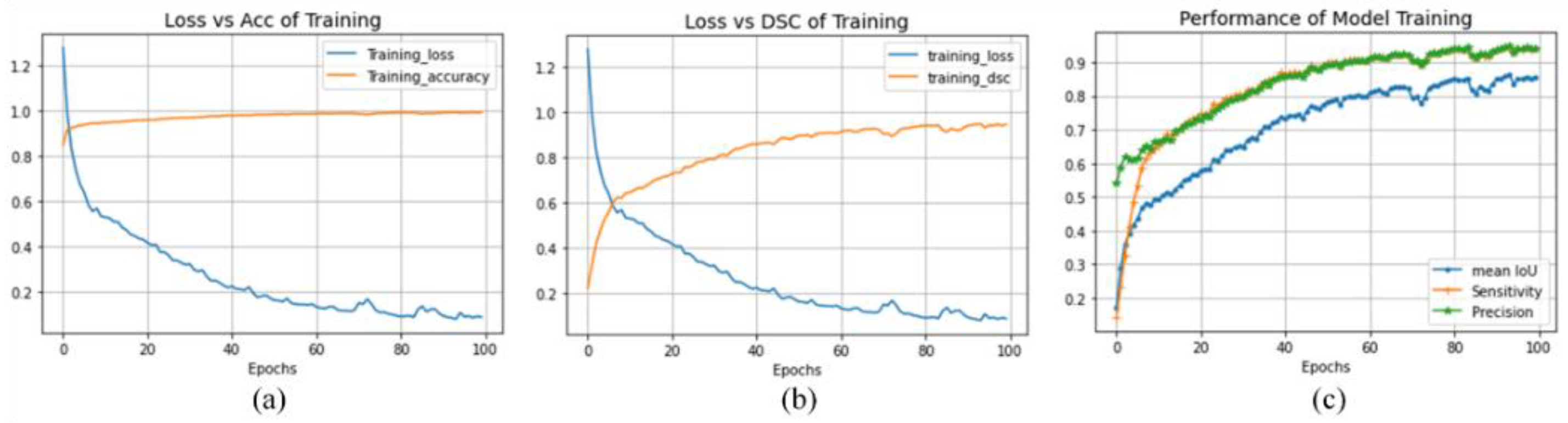
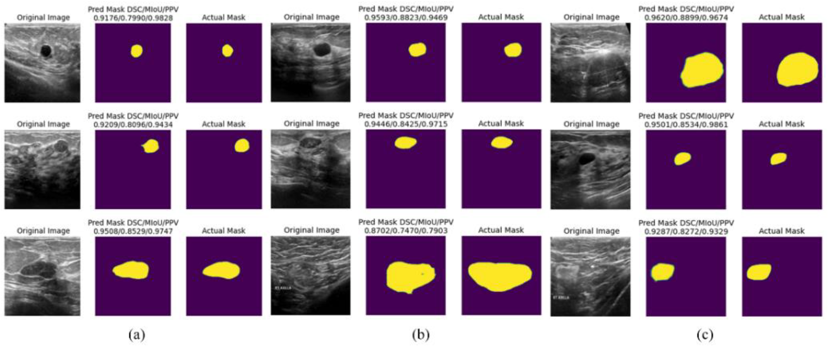
Figure 10.
The prediction results of the model under different loss functions.
4.5. Discussion
Based on the BUS2018 dataset, we use the TL method to build a FgFEU-Net model based on the U-Net model and compare the effects of different loss functions on model training and prediction. The experimental results are analyzed as follows.
Model training loss and accuracy with different loss functions. From the loss rate change curves in Figure 3 to Figure 9, we can see that the influence of different thresholds on model training changes significantly in the use of TC Loss. In all cases where the sum of α and β is 1, the point of α=β=0.5 is the best, as shown in (e) in Figure 3. In this case, TC Loss is precisely Dice Loss. In contrast, the model performance is outstanding when the sum of α and β is greater than 1, as shown in (f) in Figure 8. There is no jumping phenomenon because the loss rate of model training drops relatively smoothly. Under other loss function settings, we can conclude that the model has the best performance under the Combo loss function, as shown in Figure 9 (a).
Loss and DSC. Similarly, in the adoption of TC Loss, when α=β=0.5, the change of DSC is the best, as shown in Figure 4 (e). In contrast, the model’s performance is better when the sum of α and β is greater than 1, as shown in (f) in Figure 4. There is no jump phenomenon because the DSC rise of the model training is relatively smooth. Under other loss function settings, we can conclude that the model has the best performance under the Combo loss function, as shown in Figure 9 (b).
Model training performance. In the adoption of TC Loss, when α=β=0.5, the performance of the model is the best, as shown in (e) Figure 4, Precision is almost equal to sensitivity, but it is finally maintained at the level of 0.93. In contrast, when the sum of α and β is greater than 1, as shown in (f) in Figure 4, the performance of the model is better. Because the precision of model training rose more smoothly and reached a maximum of 0.98, sensitivity finally remained at the level of 0.93. Compared with the case of (e), the model training accuracy of (f) is greatly improved. Under other loss function settings, through the performance curve of model training, we can conclude that the performance of the model under the Combo loss function is the best, the precision rises more smoothly and gradually approaches 1, and the sensitivity is finally maintained at the level of 0.95 as shown in Figure 9 (c).
Analysis of model prediction results. From the two aspects of model prediction results and evaluation indicators, in TC loss, when α=0.70, β=0.75, the model predicts the best results, while under other loss rate functions, the model predicts the best in the case of Combo loss best results. Through comparison, we found that the BCE loss prediction rate is 0.0161, the accuracy rate is 0.9916, and the Mean IoU is 0.8654, the highest prediction among all models. In the case of combo loss, the model’s predicted loss rate is 0.0750, the accuracy rate is 0.9903, and the Mean IoU is 0.8645, second only to the case of BCE loss. Among the evaluation indicators of DSC, Sensitivity, and Precision, the model predicted the best results in the case of Combo loss, reaching 0.9802, 0.9935, and 0.9683, respectively. In the case of BCE loss, the evaluation index values of DSC, Sensitivity, and Precision reached 0.9501, 0.9690, and 0.9222, respectively, and the prediction performance was second only to the prediction performance of the model in the case of Combo loss.
On the other hand, from the model-predicted breast cancer tumor lesion mask results, the model predicted the best DSC/MIoU/PPV performance in the case of BCE Loss reaching 0.9555/0.8534/0.9967. The best performance of DSC/MIoU/PPV predicted by the model in the case of Dice loss reaches 0.9593/0.8823/0.9469. The best performance of DSC/MIoU/PPV predicted by the model under Combo loss is 0.9776/0.8350/0.9739. Therefore, the performance of our proposed model is excellent. With naked-eye visual observation, the mask predicted by our proposed model has a clear outline, and its height coincides with the lesion area of the original image, achieving the aim of breast tumor semantic segmentation. Further, Table 3 shows that our proposed FgFEU-Net model performs best in breast tumor segmentation experiments.
5. Conclusion
This paper proposes an FgFEU-Net model for tumor segmentation in breast ultrasound images based on TL. In the experiment, BUS2018 is used as the experimental dataset, the basic U-Net model as a backbone network, TC, dice, BCE, and combo loss to train and test the proposed FgFEU-Net model, and DSC/MIoU/Precision as the model to predict evaluation indicators. Experimental results indicate that the FgFEU-Net model with combo loss performs the best in model training and testing, followed by dice loss. The proposed method achieves 0.9802, 0.9683, and 0.9935 in DSC, precision, and sensitivity, respectively. In general, using the proposed model and finding a combined loss function can improve model prediction accuracy and be competent for small sample medical image segmentation without losing the model accuracy. It also solves the problem of unbalanced input and output of medical image segmentation.
Furthermore, the proposed method is compared with their enhanced models with SVM, CNN, VGG16, VGG19, LSTM, Bi-LSTM, ResNet, and DenseNet. Experimental results indicate that the proposed method performs better segmentation than the traditional model and has better segmentation performance than the basic U-Net model. Of course, our proposed method has not been experimented on other datasets. This is our future work.
Acknowledgments
This research was supported by the Natural Science Foundation Project of Jiujiang City under Grant S2024JXJJ0001, and in part by the Natural Science Foundation of Jiangxi Province under Grant 20232BAB202014, 20232BAB202053, 20232BAB202054.
References
- Guotai Wang, Wenqi Li, Maria A. Zuluaga, Rosalind Pratt, Premal A. Patel, Michael Aertsen, Tom Doel, Anna L. David, Jan Deprest, S’ebastien Ourselin, and Tom Vercauteren. Interactive medical image segmentation using deep learning with image-specific fine tuning. IEEE Transactions on Medical Imaging, 37(7):1562–1573, 2018. [CrossRef]
- Ran Gu, GuotaiWang, Tao Song, Rui Huang, Michael Aertsen, Jan Deprest, S’ebastien Ourselin, Tom Vercauteren, and Shaoting Zhang. Ca-net: Comprehensive attention convolutional neural networks for explainable medical image segmentation. IEEE Transactions on Medical Imaging, 40(2):699–711, 2021. [CrossRef]
- Annegreet Van Opbroek, M. Arfan Ikram, MeikeW. Vernooij, and Marleen de Bruijne. Transfer learning improves supervised image segmentation across imaging protocols. IEEE Transactions on Medical Imaging, 34(5):1018–1030, 2015. [CrossRef]
- Annegreet Van Opbroek, Hakim C. Achterberg, Meike W. Vernooij, and Marleen De Bruijne. Transfer learning for image segmentation by combining image weighting and kernel learning. IEEE Transactions on Medical Imaging, 38(1):213–224,2019. [CrossRef]
- Chien-Ming Lin, Chi-Yi Tsai, Yu-Cheng Lai, Shin-An Li, and Ching-Chang Wong. Visual object recognition and pose estimation based on a deep semantic segmentation network. IEEE Sensors Journal, 18(22):9370–9381, 2018. [CrossRef]
- Chaitanya Varma and Omkar Sawant. An alternative approach to detect breast cancer using digital image processing techniques. In 2018 International Conference on Communication and Signal Processing (ICCSP), pages 0134–0137, 2018.
- Etienne von Lavante and J. Alison Noble. Segmentation of breast cancer masses in ultrasound using radio-frequency signal derived parameters and strain estimates. In 2008 5th IEEE International Symposium on Biomedical Imaging: From Nano to Macro, pages 536–539, 2008.
- N Kavya, N Usha, N. Sriraam, D Sharath, and Prabha Ravi. Breast cancer detection using non invasive imaging and cyber physical system. In 2018 3rd International Conference on Circuits, Control, Communication and Computing (I4C), pages 1–4, 2018.
- Albert Gubern-M’erida, Michiel Kallenberg, Ritse M. Mann, Robert Mart’ı, and Nico Karssemeijer. Breast segmentation and density estimation in breast mri: A fully automatic framework. IEEE Journal of Biomedical and Health Informatics, 19(1):349–357, 2015. [CrossRef]
- Haeyun Lee, Jinhyoung Park, and Jae Youn Hwang. Channel attention module with multiscale grid average pooling for breast cancer segmentation in an ultrasound image. IEEE Transactions on Ultrasonics, Ferroelectrics, and Frequency Control, 67(7):1344–1353, 2020. [CrossRef]
- R. Meena Prakash, K. Bhuvaneshwari, M. Divya, K. Jamuna Sri, and A. Sulaiha Begum. Segmentation of thermal infrared breast images using k-means, fcm and em algorithms for breast cancer detection. In 2017 International Conference on Innovations in Information, Embedded and Communication Systems (ICIIECS), pages 1–4, 2017.
- Muhammed Emin Bagdigen and Gokhan Bilgin. Cell segmentation in triple-negative breast cancer histopathological images using u-net architecture. In 2020 28th Signal Processing and Communications Applications Conference (SIU), pages 1–4, 2020.
- Constance Fourcade, Ludovic Ferrer, Gianmarco Santini, No’emie Moreau, Caroline Rousseau, Marie Lacombe, Camille Guillerminet, Mathilde Colombi’e, Mario Campone, Diana Mateus, and Mathieu Rubeaux. Combining superpixels and deep learning approaches to segment active organs in metastatic breast cancer pet images. In 2020 42nd Annual International Conference of the IEEE Engineering in Medicine & Biology Society (EMBC), pages 1536–1539, 2020.
- Than Than Htay and Su Su Maung. Early stage breast cancer detection system using glcm feature extraction and k-nearest neighbor (k-nn) on mammography image. In 2018 18th International Symposium on Communications and Information Technologies (ISCIT), pages 171–175, 2018.
- Khaleel Al-Rababah, Shyamala Doraisamy, Mas Rina, and Fatimah Khalid. A color-based high temperature extraction method in breast thermogram to classify cancerous and healthy cases using svm. In 2018 2nd International Conference on Imaging, Signal Processing and Communication (ICISPC), pages 70–73, 2018.
- R. D. Ghongade and D. G.Wakde. Computer-aided diagnosis system for breast cancer using rf classifier. In 2017 International Conference on Wireless Communications, Signal Processing and Networking (WiSPNET), pages 1068–1072, 2017.
- Xiaowei Xu, Ling Fu, Yizhi Chen, Rasmus Larsson, Dandan Zhang, Shiteng Suo, Jia Hua, and Jun Zhao. Breast region segmentation being convolutional neural network in dynamic contrast enhanced mri. 2018 40th Annual International Conference of the IEEE Engineering in Medicine and Biology Society (EMBC), pages 750–753, 2018.
- Meriem Sebai, Tianjiang Wang, and Saad Ali Al-Fadhli. Partmitosis: A partially supervised deep learning framework for mitosis detection in breast cancer histopathology images. IEEE Access, 8:45133–45147, 2020. [CrossRef]
- Walid S. Al-Dhabyani, Mohammed Mohammed Mohammed Gomaa, H Khaled, and Aly A. Fahmy. Dataset of breast ultrasound images. Data in Brief, 28, 2019.
- Kaiwen Lu, Tianran Lin, Junzhou Xue, Jie Shang, and Chao Ni. An automated bearing fault diagnosis using a self-normalizing convolutional neural network. In 2019 International Conference on Quality, Reliability, Risk, Maintenance, and Safety Engineering (QR2MSE), pages 908–912, 2019.
- Zhen Huang, Tim Ng, Leo Liu, Henry Mason, Xiaodan Zhuang, and Daben Liu. Sndcnn: Self-normalizing deep cnns with scaled exponential linear units for speech recognition. In ICASSP 2020 - 2020 IEEE International Conference on Acoustics, Speech and Signal Processing (ICASSP), pages 6854–6858, 2020.
- Ngoc-Son Vu, Vu-Lam Nguyen, and Philippe-Henri Gosselin. A handcrafted normalized-convolution network for texture classification. In 2017 IEEE International Conference on Computer Vision Workshops (ICCVW), pages 1238–1245, 2017.
- Olaf Ronneberger, Philipp Fischer, and Thomas Brox. U-net: Convolutional networks for biomedical image segmentation. Computer Vision and Pattern Recognition (cs.CV), ArXiv, abs/1505.04597, 2015.
- Karen Simonyan and Andrew Zisserman. Very deep convolutional networks for large-scale image recognition. Computer Vision and Pattern Recognition (cs.CV), abs/1409.1556, 2014.
- Guotai Wang, Maria A. Zuluaga, Wenqi Li, Rosalind Pratt, Premal A. Patel, Michael Aertsen, Tom Doel, Anna L. David, Jan Deprest, S’ebastien Ourselin, and Tom Vercauteren. Deepigeos: A deep interactive geodesic framework for medical image segmentation. IEEE Transactions on Pattern Analysis and Machine Intelligence, 41(7):1559–1572, 2019. [CrossRef]
- Laura Raquel Bareiro Paniagua, Jos’e Luis V’azquez Noguera, Luis Salgueiro Romero, Deysi Natalia Leguizamon Correa, Diego P. Pinto-Roa, Julio C’esar Mello-Rom’an, Sebastian A. Grillo, Miguel Garc’ıa-Torres, Lizza A. Salgueiro Toledo, and Jacques Facon. Impact of melanocytic lesion image databases on the pre-training of segmentation tasks using the unet architecture.In 2021 XXIII Symposium on Image, Signal Processing and Artificial Vision (STSIVA), pages 1–6, 2021.
- Carole H Sudre, Wenqi Li, Tom Vercauteren, Sebastien Ourselin, and M Jorge Cardoso. Generalised dice overlap as a deep learning loss function for highly unbalanced segmentations. In Deep Learning in Medical Image Analysis and Multimodal Learning for Clinical Decision Support: Third International Workshop, DLMIA 2017, and 7th International Workshop, MLCDS 2017, Held in Conjunction with MICCAI 2017, Qu’ebec City, QC, Canada, September 14, Proceedings 3, pages 240–248. Springer, 2017.
- Loic Themyr, Cl’ement Rambour, Nicolas Thome, Toby Collins, and Alexandre Hostettler. Full contextual attention for multiresolution transformers in semantic segmentation. 2023 IEEE/CVF Winter Conference on Applications of Computer Vision (WACV), pages 3223–3232, 2022.
- Yichi Zhang, Zhenrong Shen, Rushi Jiao. Segment anything model for medical image segmentation: Current applications and future directions. Computers in Biology and Medicine, Vol.171, pages 108238, 2024.
- Jiménez-Gaona, Y.; Rodríguez-Álvarez, M.J.; Lakshminarayanan, V. Deep-Learning-Based Computer-Aided Systems for Breast Cancer Imaging: A Critical Review. Appl. Sci. 2020, 10, 8298. [CrossRef]
- Tianqi Yang, Oktay Karakus, Nantheera Anantrasirichai, and Alin Achim. Current advances in computational lung ultrasound imaging: A review. IEEE Transactions on Ultrasonics, Ferroelectrics, and Frequency Control, 70:2–15, 2021. [CrossRef]
- Stafford Michahial and Bindu A. Thomas. A novel algorithm for locating region of interest in breast ultra sound images. 2017 International Conference on Electrical, Electronics, Communication, Computer, and Optimization Techniques (ICEECCOT), pages 1–5, 2017.
- Yonghao Huang and Qinghua Huang. A superpixel-classification-based method for breast ultrasound images. 2018 5th International Conference on Systems and Informatics (ICSAI), pages 560–564, 2018.
- Zhao Yu-qian, Gui Wei-hua, Chen Zhen-cheng, Tang Jing-tian, and Li Ling-yun. Medical images edge detection based on mathematical morphology. 2005 IEEE Engineering in Medicine and Biology 27th Annual Conference, pages 6492–6495, 2005.
- M. Lalonde, M. Beaulieu, and L. Gagnon. Fast and robust optic disc detection using pyramidal decomposition and hausdorffbased template matching. IEEE Transactions on Medical Imaging, 20(11):1193–1200, 2001. [CrossRef]
- Wenan Chen, Rebecca Smith, Soo-Yeon Ji, Kevin RWard, and Kayvan Najarian. Automated ventricular systems segmentation in brain ct images by combining low-level segmentation and high-level template matching. BMC medical informatics and decision making, 9 Suppl 1:S4, November 2009. [CrossRef]
- A. Tsai, A. Yezzi, W. Wells, C. Tempany, D. Tucker, A. Fan, W.E. Grimson, and A. Willsky. A shape-based approach to the segmentation of medical imagery using level sets. IEEE Transactions on Medical Imaging, 22(2):137–154, 2003. [CrossRef]
- Changyang Li, XiuyingWang, Stefan Eberl, Michael Fulham, Yong Yin, Jinhu Chen, and David Dagan Feng. A likelihood and local constraint level set model for liver tumor segmentation from ct volumes. IEEE Transactions on Biomedical Engineering, 60(10):2967–2977, 2013. [CrossRef]
- S. Li, T. Fevens, and Adam Krzy˙zak. A svm-based framework for autonomous volumetric medical image segmentation using hierarchical and coupled level sets. In Computer Assisted Radiology and Surgery - International Congress and Exhibition, 2004.
- Saeid Asgari Taghanaki, Yefeng Zheng, Shaohua Kevin Zhou, Bogdan Georgescu, Puneet S. Sharma, Daguang Xu, Dorin Comaniciu, and G. Hamarneh. Combo loss: Handling input and output imbalance in multi-organ segmentation. Computerized medical imaging and graphics : the official journal of the Computerized Medical Imaging Society, 75:24–33, 2018.
- Xiaoya Li, Xiaofei Sun, Yuxian Meng, Junjun Liang, Fei Wu, and Jiwei Li. Dice loss for data-imbalanced NLP tasks. In Proceedings of the 58th Annual Meeting of the Association for Computational Linguistics, pages 465–476, Online, Jul 2020. Association for Computational Linguistics.
- Yaoshiang Ho and Samuel Wookey. The real-world-weight cross-entropy loss function: Modeling the costs of mislabeling. IEEE Access, 8:4806–4813, 2020. [CrossRef]
- Sheetal Janthakal and Girisha Hosalli. A binary cross entropy u-net based lesion segmentation of granular parakeratosis. In 2021 International Conference on Advancements in Electrical, Electronics, Communication, Computing and Automation (ICAECA), pages 1–7, 2021.
- Haonan Wang, Peng Cao, Jiaqi Wang, and Osmar R Zaiane. Uctransnet: Rethinking the skip connections in u-net from a channel-wise perspective with transformer. In AAAI Conference on Artificial Intelligence, 2021. [CrossRef]
- Fenglin Liu, Xuancheng Ren, Zhiyuan Zhang, Xu Sun, and Yuexian Zou. Rethinking skip connection with layer normalization in transformers and resnets. Machine Learning (cs.LG), ArXiv, abs/2105.07205, 2021.
- Kaiming He, Xiangyu Zhang, Shaoqing Ren, and Jian Sun. Deep residual learning for image recognition. In 2016 IEEE Conference on Computer Vision and Pattern Recognition (CVPR), pages 770–778, 2016.
- Fabian Isensee, Paul F. Jager, Simon A. A. Kohl, Jens Petersen, and Klaus Maier-Hein. Automated design of deep learning methods for biomedical image segmentation. Computer Vision and Pattern Recognition (cs.CV), arXiv: Computer Vision and Pattern Recognition, 2019.
- Seyed Sadegh Mohseni Salehi, Deniz Erdo˘gmus¸, and Ali Gholipour. Tversky Loss Function for Image Segmentation Using 3D Fully Convolutional Deep Networks. In: Wang, Q., Shi, Y., Suk, HI., Suzuki, K. (eds) Machine Learning in Medical Imaging. MLMI 2017. vol 10541, 2017.
- Michael Yeung, Evis Sala, Carola-Bibiane Sch¨onlieb, and Leonardo Rundo. Unified focal loss: Generalising dice and cross entropy-based losses to handle class imbalanced medical image segmentation. Computerized Medical Imaging and Graphics, 95, 2021.
- Liangliang Liu, Jianhong Cheng, Quan Quan, Fang-Xiang Wu, Yu-Ping Wang, and Jianxin Wang. A survey on u-shaped networks in medical image segmentations. Neurocomputing, 409:244–258, 2020. [CrossRef]
- Jo Schlemper, Ozan Oktay, Michiel Schaap, Mattias P. Heinrich, Bernhard Kainz, Ben Glocker, and Daniel Rueckert. Attention gated networks: Learning to leverage salient regions in medical images. Medical image analysis, 53:197 – 207, 2018. [CrossRef]
- Fausto Milletari, Nassir Navab, and Seyed-Ahmad Ahmadi. V-net: Fully convolutional neural networks for volumetric medical image segmentation. In 2016 Fourth International Conference on 3D Vision (3DV), pages 565–571, 2016.
- Hoel Kervadec, Jihene Bouchtiba, Christian Desrosiers, Eric Granger, Jos’e Dolz, and Ismail Ben Ayed. Boundary loss for highly unbalanced segmentation. Medical image analysis, 67:101851, 2018. [CrossRef]
- Antonio Galli, Stefano Marrone, Gabriele Piantadosi, Mario Sansone, and Carlo Sansone. A pipelined tracer-aware approach for lesion segmentation in breast dce-mri. Journal of Imaging, 7(12), 2021. [CrossRef]
- Kaiwen Yang, Aiga Suzuki, Jiaxing Ye, Hirokazu Nosato, Ayumi Izumori, and Hidenori Sakanashi. Ctg-net: Cross-task guided network for breast ultrasound diagnosis. PloS one, 17(8):e0271106, 2022. [CrossRef]
- Bendeg’uz H Zov’athi, R’eka Moh’acsi, Attila Marcell Sz’asz, and Gy¨orgy Cserey. Breast tumor tissue segmentation with areabased annotation using convolutional neural network. Diagnostics, 12(9):2161, 2022.
- Xianjun Fu, Hao Cao, Hexuan Hu, Bobo Lian, Yansong Wang, Qian Huang, and Yirui Wu. Attention-based active learning framework for segmentation of breast cancer in mammograms. Applied Sciences, 13(2):852, 2023. [CrossRef]
- Anu Singha and Mrinal Kanti Bhowmik. Alexsegnet: an accurate nuclei segmentation deep learning model in microscopic images for diagnosis of cancer. Multimedia Tools and Applications, 82(13):20431–20452, 2023. [CrossRef]
- Anusua Basu, Pradip Senapati, Mainak Deb, Rebika Rai, and Krishna Gopal Dhal. A survey on recent trends in deep learning for nucleus segmentation from histopathology images. Evolving Systems, pages 1–46, 2023. [CrossRef]
- Xuejian Li, Shiqiang Ma, Junhai Xu, Jijun Tang, Shengfeng He, Fei Guo. TranSiam: Aggregating multi-modal visual features with locality for medical image segmentation. Expert Systems with Applications, vol.237, pages 121574, 2024. [CrossRef]
- Yongjian Wu, Xiaoming Xi, Xianjing Meng, Xiushan Nie, Yanwei Ren, Guang Zhang, Cuihuan Tian, and Yilong Yin. Label-distribution learning-embedded active contour model for breast tumor segmentation. IEEE Access, 7:97857–97864, 2019. [CrossRef]
- Kexin Ding, Mu Zhou, HeWang, Olivier Gevaert, Dimitris Metaxas, and Shaoting Zhang. A large-scale synthetic pathological dataset for deep learning-enabled segmentation of breast cancer. Scientific Data, 10(1):231, 2023. [CrossRef]
Figure 1.
U-Net model architecture for breast tumor segmentation.
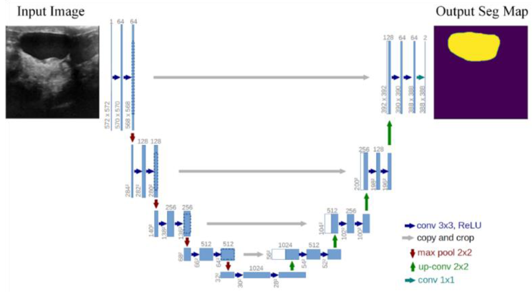
Figure 2.
The architecture of the proposed FgFEU-Net model based on TL.
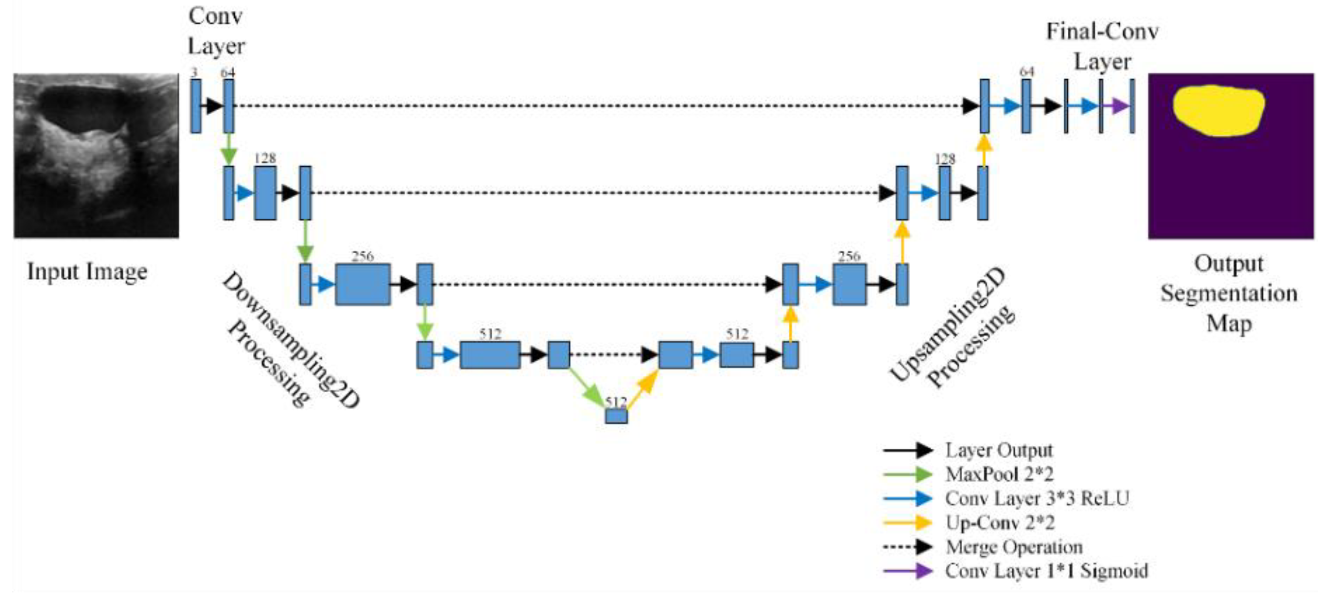

Table 1.
Model Test Loss-Accuracy using TC loss, BCE loss, Dice loss, and Combo.
| Loss Function | Model Prediction Evaluation | |||
|---|---|---|---|---|
| Penalty Coefficient | ||||
| TC Loss | α | β | Loss | Accuracy |
| 0.5 | 0.5 | 0.0602 | 0.9876 | |
| 0.4 | 0.6 | 0.0746 | 0.9848 | |
| 0.3 | 0.7 | 0.0988 | 0.9777 | |
| 0.2 | 0.8 | 0.0549 | 0.9801 | |
| 0.1 | 0.9 | 0.0956 | 0.9612 | |
| 0.7 | 0.75 | 0.0537 | 0.9866 | |
| BCE Loss | 0.0161 | 0.9916 | ||
| Dice Loss | 0.0874 | 0.9836 | ||
| Combo Loss | 0.0750 | 0.9903 | ||
Table 2.
Evaluation metrics using TC loss, BCE loss, Dice loss, and Combo loss in model prediction.
| Loss Function | Model Prediction Evaluation | |||||
|---|---|---|---|---|---|---|
| Penalty Coefficient | ||||||
| TC Loss | α | β | DSC | MIOU | Sensitivity | Precision |
| 0.5 | 0.5 | 0.9400 | 0.8456 | 0.9436 | 0.9368 | |
| 0.4 | 0.6 | 0.9160 | 0.8163 | 0.9692 | 0.8702 | |
| 0.3 | 0.7 | 0.9015 | 0.7414 | 0.9435 | 0.8194 | |
| 0.2 | 0.8 | 0.8903 | 0.7742 | 0.9863 | 0.8119 | |
| 0.1 | 0.9 | 0.7635 | 0.5993 | 0.9496 | 0.6398 | |
| 0.7 | 0.75 | 0.9356 | 0.8346 | 0.9097 | 0.9632 | |
| BCE Loss | 0.9501 | 0.8654 | 0.9690 | 0.9222 | ||
| Dice Loss | 0.9138 | 0.8083 | 0.9556 | 0.8773 | ||
| Combo Loss | 0.9802 | 0.8645 | 0.9935 | 0.9683 | ||
Table 3.
The lesion evaluation metrics of the proposed model are compared with methods in the literature in the breast tumor segmentation experiments. In comparative experiments, we compare the commonly used medical tumor segmentation models in the references, including CNN, VGG, LSTM, Bi-LSTM, ResNet, DenseNet, the currently popular U-Net model, and their enhanced models. The evaluation indicators of the comparative experiments include the loss and accuracy during model training and testing, respectively.
| Model | Loss | Accuracy | F1 | ROC | ||
|---|---|---|---|---|---|---|
| Training | Test | Training | Test | |||
| SVM | 0.1325 | 0.1589 | 0.9832 | 0.9829 | 0.9829 | 0.9876 |
| CNN | 0.4088 | 0.5516 | 0.7474 | 0.7924 | 0.7862 | 0.9016 |
| VGG16 | 0.4363 | 0.7057 | 0.9017 | 0.7350 | 0.7322 | 0.8645 |
| VGG16_Enhanced | 0.0315 | 0.0751 | 0.9866 | 0.9573 | 0.9567 | 0.9819 |
| VGG19 | 0.7640 | 0.5889 | 0.9480 | 0.7607 | 0.7571 | 0.8937 |
| VGG19_Enhanced | 0.1016 | 0.1519 | 0.9866 | 0.9573 | 0.9576 | 0.9879 |
| LSTM | 0.2457 | 0.8186 | 0.8859 | 0.7761 | 0.6855 | 0.6838 |
| Bi-LSTM | 0.1105 | 0.7648 | 0.9732 | 0.8034 | 0.7999 | 0.8034 |
| ResNet50 | 0.1574 | 0.2764 | 0.9782 | 0.9573 | 0.9570 | 0.9903 |
| DenseNet121 | 0.1774 | 0.2392 | 0.9285 | 0.9159 | 0.9126 | 0.9215 |
| U-Net | 0.0756 | 0.1985 | 0.9861 | 0.9656 | 0.9602 | 0.9762 |
| FgFEU-Net (Ours) | 0.0161 | 0.0874 | 0.9916 | 0.9836 | 0.9815 | 0.9906 |
Disclaimer/Publisher’s Note: The statements, opinions and data contained in all publications are solely those of the individual author(s) and contributor(s) and not of MDPI and/or the editor(s). MDPI and/or the editor(s) disclaim responsibility for any injury to people or property resulting from any ideas, methods, instructions or products referred to in the content. |
© 2025 by the authors. Licensee MDPI, Basel, Switzerland. This article is an open access article distributed under the terms and conditions of the Creative Commons Attribution (CC BY) license (http://creativecommons.org/licenses/by/4.0/).
Copyright: This open access article is published under a Creative Commons CC BY 4.0 license, which permit the free download, distribution, and reuse, provided that the author and preprint are cited in any reuse.


