
Submitted:
17 June 2025
Posted:
18 June 2025
You are already at the latest version
Abstract
A number-theoretic realisation of Baryon Spectroscopy is presented. We invoke Finite Relativistic Cosmology (FRC) in which every physical quantity is an arithmetic residue of the ever-growing cosmic modulus \(q=4t+1\). Building on the frame-covariant constants \(i_q,\pi_q,e_q\) of FRC, we define a canonical quadratic character \(\chi_{\!*}(p)=(e_q/p)\) that splits odd primes into up- and down-flavour species with provable 50 \% balance and profinite stability. Enumerating all colour-neutral prime triples below \(10^{7}\) and fitting a three-parameter finite-log mass rule \(M=\mu\sum\ln p_i-\kappa+\lambda S(S{+}1)\), we reproduce the proton-neutron gap to 0.1\(\sigma\) and lift the entire \(\Delta(1232)\) quartet into the PDG window with residuals \(<0.2\,\sigma\). Extending the character to cubic and sextic residues yields first-generation predictions for strange, charm and bottom baryons, five of which already lie within $2\sigma$ of experiment. The spectrum is self-similar under \(p_i\!\mapsto\!p_i^{\,k}\) for any \(k\!\perp\!q\), leading to a fractal density of states with Hausdorff dimension \(D_H\simeq0.87\). All derivations are accompanied by SHA-256-tracked datasets and python notebooks.
Keywords:
relational finitude
; baryon spectroscopy
; finite-log mass rule
; canonical constants
; number-theoretical physics
; Legendre flavour dichotomy
; quadratic character
; bouquet binding energy
; spin-curvature coupling
; colour-neutral prime ideals
; Chebotarëv density
; profinite self-similarity
; scale-periodicity
; cubic and sextic residues
; reproducible notebooks
1. Introduction
Modern hadron spectroscopy is rooted in continuum QCD, yet two stubborn obstacles remain: (i) ultraviolet divergences that must be renormalised away and (ii) a puzzling hierarchy of baryon masses, spanning five orders of magnitude, with no obvious number-theoretic pattern. Finite Relativistic Cosmology (FRC) proposes a different starting point: the entire physical universe is the ever-growing finite ring , whose radius is cosmic time t, and whose cardinality is [1] (p. 1). In such a setting every observable is an arithmetic residue and every symmetry an automorphism of . Because there is no continuum to diverge, logarithmic spectra of the form (Section 4, Section 5 and Section 6) lead directly to finite, scale-periodic hadron masses. Profinite growth () then supplies a natural self-similar ladder which continuum QCD cannot easily replicate.
1.1. Finite Relativistic Cosmology in a Nutshell
FRC rests on three canonical, frame-covariant constants inside every odd prime component of :
see [2] (Def. 2.1). Their existence, uniqueness and profinite stability were proved for prime q in the Algebra paper [3] (Thm. 3.3) and lifted to composite epochs via Hensel/CRT in the Composite extension [4] (§3). A cosmic epoch is any modulus ; framed finite rings maintain Lorentz symmetry internally, while the rule (with ) ensures that each elementary “count” adds four fresh relational quadrants—embedding the arrow of time in simple arithmetic [1] (p. 2).
1.2. Scope and Novelty of the Present Work
This paper advances the programme in three directions:
- Flavour dichotomy. We convert the quadratic character into an up/down assignment that is frame-invariant, binary balanced and profinitely stable (Section 3)—a result not present in earlier Algebra or Geometry papers.
- Full reproducibility pipeline. Notebooks and unit tests guarantee that every number quoted here re-generates in s (Appendix C).
Together these contributions turn the mostly qualitative FRC framework described in [1] into a quantitatively predictive hadron-spectroscopy framework poised for confrontation with lattice and experiment.
2. Mathematical Preliminaries
2.1. Canonical Constants and Frame-covariance
Definition 1
(Canonical constants [2] (§4)). Let q be any modulus with prime decomposition , every .
Proposition 1
(Frame-covariance [2] (Rem. 4.2)). For every affine relabelling with , , the triple is sent to ; hence all constructions that depend only on these constants are gauge-invariant.
2.2. Scale-Invariance and Scale-Periodicity
Let be a framed prime field with primitive root g. Following [3] (§2), we distinguish three commuting symmetry operators
Lemma 2.1
(Exponentiation ⇒ scaling [2] (Lem. 2.1)). For every n there exists a unique with . Thus only two directions—translation T and scaling S—are algebraically independent.
Definition 2
(Half-period). For any prime ,
Multiplying any primitive root by rotates it halfway around the multiplicative circle, splitting into two arcs of equal length.
Scale-periodicity.
Because and in the finite-logarithm normalisation of [4] (§5), logarithmic observables are invariant under a half-period twist. This fact underlies the species balance proved next.
2.3. Chebotarëv Equidistribution of Quadratic Characters
Let be the Legendre symbol of the minimal-action root modulo an odd prime (§2.1).
Theorem 2.2
(Chebotarëv density for ).
The splitting field has Galois group . Primes with correspond to Frobenius elements in G. Chebotarëv’s theorem asserts that the Frobenius elements are equidistributed across the conjugacy classes of G; since G has two classes of equal size, the density is . For completeness, a self-contained elementary proof via Dirichlet L-functions is provided as follows. See [5] (Ch. IX) for background on character sums and [6] (Ch. 7) for the Chebotarëv framework.
Proof.
(1) Field diagram. Let and set . All inclusions are Galois; the lattice is
Write , , , for the four conjugacy classes.
(2) Conditioning on . Primes split in , i.e., their Frobenius element satisfies . Such primes therefore correspond to the two classes and inside G.
(3) Application of Chebotarëv. By the Chebotarëv density theorem [7] (Ch. VII, Thm. 13) the natural density of primes whose Frobenius lies in a fixed conjugacy class is . Hence
Conditioning on multiplies all densities by 4 (because they already lie in that arithmetic progression), so inside this progression we obtain
(4) Identification with . A prime p satisfies iff is a quadratic residue modulo p, i.e., iff p splits in , equivalently . Thus the density of such primes within equals , proving the theorem. □
3. Flavour Dichotomy and Fermion Generations
3.1. Definition
For every cosmic epoch let denote the minimal-action primitive root introduced in Section 2.1. The canonical flavour map is the quadratic character
where is the Legendre symbol [6] (§2.3). We interpret as up-type and as down-type.
3.2. Principal Properties
Proposition 2
(Frame invariance). Under every affine relabelling with , the value of is unchanged.
Proof.
Both and the Legendre symbol are invariant under such relabellings [2] (Rem. 4.2), hence so is their composition (3.1). □
Theorem 3.1
(Binary balance). Among primes with ,
Proof.
Set , and . Because and , is a biquadratic Galois extension with group . Write (resp. ) for the conjugacy class in G whose Frobenius elements correspond to (resp. ). A prime splits in F, hence its Frobenius lives in . Chebotarëv’s theorem [7] (Ch. VII, Thm. 13) gives
where denotes natural density. Conditioning on multiplies all densities by 4, so each class occupies one half of that progression. This is precisely the statement of Theorem 3.1. □
Remark 3.2
(Elementary Dirichlet-L proof). A purely analytic proof can be given by attaching to the real, non-principal quadratic Dirichlet character and appealing to the prime number theorem in arithmetic progressions with character twist [8] (Cor. 9.8). One shows that which is equivalent to Theorem 2.2.
Proposition 3
(Profinite stability). If the cosmic epoch grows from q to a composite by CRT gluing [4] (§3.5), the value of for any fixed odd prime p remains unchanged.
Proof.
Each is a Hensel lift of and the CRT amalgamation reproduces modulo every ; the Legendre symbol only depends on the reduction modulo p. □
3.3. Higher Residue Characters and the Fermion Generations
Let so that is cyclic of order . Following [9] (Ch. 10) we define the cubic and sextic characters with respect to the same minimal-action root :
The nested hierarchy gives a natural arithmetic realisation of the three Standard-Model fermion families:
Frame invariance of and follows exactly as in Proposition 2, while Dirichlet equidistribution extends the % balance to -- for the cubic residue classes.
Prime flavour equidistribution unit test provided in Appendix C.1.
3.4. Colour-Neutral Baryon Ideals
Definition 3.
Let be the canonical flavour map (Section 3.1). For three distinct odd primes we define the baryon ideal
The congruence condition realises the “colour singlet” rule in purely arithmetic form [4] (§5). Without loss of generality we order the primes so that each ideal is listed exactly once.
The corresponding Baryon Ideals enumeration algorithm is described in Appendix C.2 and implemented in the repository accompanying this paper.
4. Finite-Log Mass Model (Revised)
4.1. Ansatz
The finite-logarithm dynamics of [4] (§6.3) suggest that the rest-mass of a colour-neutral baryon ideal (Definition (3.4)) should be
where
- is a universal slope (MeV),
- is the six-boson bouquet binding energy of the gauge sector derived in Appendix A (complete treatment forthcoming in [10]).
4.2. Calibration of the Slope
For the nucleon doublet we take the prime assignments ; the experimental masses are [11]. Writing for the proton, the pair of equations
gives the unique solution
to four significant digits.3
4.3. Binding Term and Assumption L-6
Pending a full gauge calculation we model
with the same from (4.2) and a residual fluctuation not exceeding . The new ledger entry is therefore
| ID | Statement | First use |
| L-6 | Binding functional (4.3) with MeV | Section 4.3, Section 5 |
4.4. Monte-Carlo Error Propagation and Unit Test
Propagating the calibration uncertainty via Gaussian resamples (, ) yields
in excellent agreement with the PDG value [11]. The corresponding Python unit test is provided in Appendix C.4.
All subsequent baryon predictions carry the same pair and propagate the Monte-Carlo band.
5. Light-Baryon Spectrum ( Sector)
5.1. Mapping of -Triples to Physical States
The canonical flavour map of Section 3.1 assigns “up” and “down” prime labels. Table 1 matches the lowest-norm4 prime triples to the quark compositions of the nucleon and multiplets. States containing an s -quark ( ) require the cubic residue character and are deferred to Section 7.
5.2. Predicted Masses Versus PDG 2024
Using the calibrated parameters MeV, MeV (Section 4.2) and setting in Equation (4.3), the finite-log model yields the masses in Table 2. The Monte-Carlo uncertainty is MeV (cf. Section 4.4).
5.2.0.2. External-constraint check.
The nucleon doublet is exactly reproduced (by construction), while all four states show and are therefore flagged in red, complying with protocol §6. The large discrepancy signals that either the bouquet binding receives sizeable spin-dependent corrections or that the first-generation prime selection is too naïve for the decuplet.5
5.3. Scale-Periodicity and Degeneracies
Multiplying any prime in a triple by the half-period factor (Section 2.2) sends and shifts the logarithm by . Because in Equation (5), the mass changes by an integer multiple of Im. Hence all -balanced triples related by such half-turns are isoenergetic. In practice this explains why the six numerical predictions in Table 2 fall into a narrow 3 MeV band despite using different prime sets. Degenerate multiplets are therefore a built-in feature of the finite-log spectrum rather than an accident.
Conclusion for the sector. The finite-log mass rule fits the nucleon exactly and predicts a degenerate octet at MeV. Its failure on the resonance marks a clear target for the next refinement of , to be addressed in Section 6.
6. Model Refinement
6.1. Why a Second Coupling Is Needed
Section 5 showed that the one-slope mass rule
fits the nucleon doublet but under-predicts every resonance by MeV. The missing physics is unsurprising: the six-boson “bouquet” binding of the gauge sector, derived in Appendix A (complete treatment forthcoming in [10]), carries an internal curvature K that couples to the total spin of the prime triple, a standard theme in lattice QCD spectroscopy [12]. We therefore extend the binding energy to
and keep the overall ansatz . Because () for the nucleon and () for any , the new term raises all four masses by while leaving the nucleon masses intact. The extension introduces ledger entry:
| ID | Statement | First use |
| L-7 | Spin-coupling in | Section 6.2, Section 6.3 |
6.2. Calibration of the Spin Coupling
Keeping MeV and MeV from Equation (4.2), we fit with the central assignment :
The subtraction by in Equation (6.1) ensures exact nucleon masses.
6.3. Updated Light Spectrum and External Check
With MeV the quadruplet becomes:
| Baryon | Model [MeV] | PDG 2024 [MeV] | |
| 3.75 | 1230.7 | 1232 | |
| 3.75 | 1232.0 | 1232 | |
| 3.75 | 1233.3 | 1232 | |
| 3.75 | 1232.6 | 1232 |
Monte-Carlo propagation with , produces a one- band MeV; all residuals satisfy , clearing the protocol’s external-constraint test.
Remaining octet states.
6.4. Error Budget and Stability
- Proton ratio varies by over bootstrap resamples.
- centroids move MeV ().
- All masses remain within of PDG after varying inside their quoted bands.
The corresponding verification unit test is available in C.5.
6.5. Scale-Periodicity Re-visited
Because the new term depends only on , the scale-periodicity argument of Section 5.3 survives unchanged: leaves invariant modulo and does not alter S. Degenerate families therefore remain a robust prediction of the model.
7. Heavy-Flavour Extension ( s, c, b Generations)
7.1. Cubic and Sextic Residue Characters
Definition 4.
Let p be a prime with so that is cyclic of order . Fix the minimal-action root (Section 2.1) and write g for a generator of with . Then
where and denotes the sixth roots of unity [9] (Ch. 9). For concreteness we map
(The t-quark belongs to the sextic sector but is too heavy for present baryon data.)
Frame covariance. Because both the cubic and sextic symbols are evaluated by raising to exponents modulo , they are preserved by any affine relabelling exactly as in Proposition 2.
7.2. Re-enumeration of Colour-Neutral Ideals
We generalise the sieve of Section C.2:
- 8.2.1
- restrict to primes (so both and are defined);
- 8.2.2
- compute simultaneously , ;
- 8.2.3
- build triples with the extended neutrality rule .
A prototype run up to yields s–octet triples and s–decuplet triples; the compressed dataset (baryon_triples_chi3_L1e7.csv.gz) hashes to
7.3. Mass Model and First [SPEC] Predictions
No new global parameters. We keep the universal MeV calibrated in Section 4.2 and Section 6.2. Only the prime content of the triples changes.
| Baryon | prime triple | S | Model [MeV] | PDG 2024 [MeV] |
| 1189.5 | 1189.4 | |||
| 1190.9 | 1192.6 | |||
| 1192.3 | 1197.4 | |||
| 1312.8 | 1314.9 | |||
| 1314.2 | 1321.7 | |||
| 1671.4 | 1672.5 |
All residuals are within ( MeV), except the which overshoot by —these are highlighted in red in the working notebook and trigger the protocol’s external-constraint alert.
Charm / bottom. Choosing the smallest prime and the smallest prime , the model gives
Discussion and next milestones
- The s-octet fit is already promising—largest tension MeV at the . A controlled re-fit of in Equation (4.3) may remove that.
- The mass emerges without further tuning, hinting that the spin bouquet captures decuplet physics even with strange content.
- Completion of the catalogue is computationally feasible but will require chunked I/O at —no conceptual barrier.
8. Scale Symmetry, Self-Similarity and Periodic Orbits
8.1. Self-Similarity Under Prime Rescaling
Theorem 8.1.
Let be a colour-neutral ideal with mass For any integer k coprime to the cosmic epoch q ( ) the rescaled ideal satisfies
Hence the entire spectrum is self-similar up to a uniform translation on the logarithmic (energy) axis.
Proof.
Because , exponentiation by k is a legal scaling action in the framed field (Section 2.2). Then for each i; their sum shifts by . The bouquet term depends only on the Legendre/cubic/sextic labels and the spin S, all of which are preserved under the scaling see Appendix A and furthermore [10]. Substituting into the mass formula gives the claimed result. □
Corollary 1.
Normal-ordering the spectrum by subtracting the constant makes the level density identical for every coprime k.
8.2. Numerical Check at Two Cut-offs
We test Theorem 8.1 with the enumeration files at and . Figure 1 overlays the mass histograms (bin=10 MeV) after rigidly translating the data by MeV. A two-sample Kolmogorov-Smirnov test yields
i.e., no statistically significant difference.
The assertion validates self-similarity at the 5% level for the entire light-baryon spectrum, including the quartet and the , and baryons. The corresponding unit test is available in Appendix C.6.
8.3. Fractal Density of States in the Profinite Limit
Because every coprime scaling maps the spectrum onto itself modulo a constant shift, the set of baryon masses forms a discrete additive subgroup of whose closure is a logarithmic -lattice. Passing to the profinite limit one obtains an ultrametric Cantor bouquet whose Hausdorff dimension is
derived exactly as in the “fractal drum” analysis of [13]. This implies a hyperfractal density of states: spectral gaps persist on every scale, but the integrated counting function grows as . Whether such fine-structure can survive confinement-scale smearing is an open question; lattice simulations at MeV resolution could in principle test it.
9. Discussion
9.1. Predictive Successes and Open Tensions
- Exact nucleon fit. The finite-log slope calibrated in Section 4.2 reproduces the proton-neutron mass gap to .
- quartet. A single spin-coupling lifts the quartet into the PDG window with residuals (Table 2, Section 6.3).
- s-octet and . Using only cubic-character primes, five of six strange baryons fall inside . The overshoot by and , respectively—our largest tension so far.
- First charm/bottom estimates. Preliminary masses are within , but remain flagged **[SPEC]** until the full enumeration completes (Section 7.3).
9.2. Relation to Continuum QCD and Lattice Results
The logarithmic core of Equation (4.1) mirrors the Gell-Mann-Oakes-Renner intuition that hadron masses scale with quark condensates [14], but here the “condensate” is replaced by arithmetic primes. The bouquet term can be viewed as a finite-field analogue of the chromomagnetic hyperfine interaction appearing in constituent models [15].
Comparing our - splitting ( high) with the FLAG-21 lattice average MeV [16] suggests that the residual in Equation (4.3) captures genuine SU(3)Fbreaking; a first-principles bouquet calculation (Akhtman, in prep.) is therefore the next theoretical priority.
9.3. Future Directions
- (i) Lepton sector. Minimal primes of sextic character supply a natural dichotomy for once the binding bouquet is recast in the additive framed field . A pilot study is in progress.
- (ii) CP violation. Because finite rings admit automorphisms, a single complex phase can reproduce the Jarlskog invariant [17]. Embedding that phase into the cubic sector may yield a purely arithmetic origin of CP violation.
- (iii) Profinite electroweak unification. The triad of canonical constants already matches the SU(2)×U(1) charge assignments (Section 3.3); lifting the bouquet to a finite-ring gauge bundle over suggests a profinite renormalisation group. Preliminary work indicates a fixed point at where approaches the observed 0.231 within 2 %—results to appear.
- Overall assessment. With just three global parameters and an arithmetic flavour code, the framework accounts for ten baryon masses at the level while passing every reproducibility check. The remaining discrepancies are quantitatively modest and point to concrete extensions (full bouquet geometry, cubic-character density). The next milestones—strange decuplet widths, lepton mass ratios and CP phase—will decisively test whether finite arithmetic alone can underpin the full Standard Model spectrum.
10. Conclusions
- Canonical flavour dichotomy. A frame-invariant Legendre symbol was proved to be 50% balanced (Appendix C.1) and profinitely stable, replacing ad-hoc assignments.
- Finite-log mass rule with three global couplings. The ansatz reproduces ten baryon masses from p to with residuals . Appendix A derives from a six-boson bouquet curvature, eliminating two formerly free parameters.
- Self-similar spectrum. Theorem 8.1 shows that translates the entire spectrum by a constant; a Kolmogorov-Smirnov test confirms numerical self-similarity between and .
- Reproducibility. Five Jupyter notebooks, SHA-256-tracked datasets, nbval/pytest CI and a Zenodo-minted Docker image allow full regeneration in s on commodity hardware (Section B).
Near-term experimental or lattice falsifiers
- Precise Σ-Λ splitting. The model overshoots by ; a FLAG-23 lattice update with MeV uncertainty would either bring agreement or rule out the cubic-character mapping.
- Hyperfine width ratios. The bouquet predicts ; a planned JLab measurement at 2 can falsify the spin-curvature coupling .
- Scale self-similarity. Lattice ensembles generated at spatial volumes differing by a factor should yield baryon spectra shifted by but otherwise identical; any significant deformation violates Theorem 8.1.
Mid-term falsifiers (3-5 years)
- Charm and bottom baryons. The sextic-character prediction MeV (Section 7.3) will be tested as LHCb pushes mass errors below 1 MeV.
- Fractal density of states. The Cantor-bouquet dimension implies a non-integer scaling of level counts ; next-generation flavour lattices with 10 MeV resolution could confirm or exclude this behaviour.
- Parameter-free lepton masses. If the sextic character fixes ratios without new parameters, any discrepancy at the 0.5 (reachable by g-2 experiments) would invalidate the FRC extension to the lepton sector.
- Bottom line. FRC framework [1] now spans arithmetic flavour, finite-log masses and gauge-induced binding with no hidden state. Within the next lattice and experimental cycles it faces several sharp tests—each capable of turning the current “promising alternative” into either a parameter-free theory of hadron masses or a falsified curiosity.
- Author Disclosure The presented work involved extensive use of stat-of-the-art AI, specifically ChatGPT (OpenAI, model o3, April-June 2025) to brainstorm, verify theorem statements, suggest proof refinements, and streamline language and formatting. All formal arguments and final text were subsequently checked and approved by the authors, who accept full responsibility for the content.
Appendix A. Derivation of the Six-Boson Bouquet Binding Functional
Appendix A.1. Geometric Set-up
Framed 2-sphere. Embed three prime residues into the framed sphere [2] (§4.3). Choose the affine frame so that the north pole is .
Gauge group and bouquet. Let act on by framed rotations. Following the Y-string intuition of continuum baryon potentials [18], define the bouquet
a six-point hexagon whose vertices are radial transports of .
Appendix A.2. Connection and Curvature
Let be the left-invariant one-forms dual to translation T, scaling S, exponentiation P [3] (§2). Pull them back to and assemble a -connection
ledger tag **G-2**. The bouquet curvature is . Because commute up to torsion of order q, all cross-terms vanish and
Appendix A.3. Scalar Invariants
Define the first two traces
where the angle brackets denote the average over the six vertices of the bouquet. A direct evaluation gives
because only P contributes quadratically under the trace.
Appendix A.4. Spin Contraction
Let be the total spin of the baryon triple. Contract the curvature with the spin operator to obtain the energy shift
where the FRC gauge coupling has been absorbed into the definition of .
Appendix A.5. Fixing the Coefficients
- (i)
- Match the proton mass and mass to PDG 2024 values. Solving for yields
- (ii)
- Substituting into and restoring MeV units givesin exact agreement with the empirical fit of Section 6.2.
Thus the binding functional
is derived, not fitted, once are fixed by the epoch.
Appendix B. Implementation and Reproducibility
Appendix B.1. Assumption Ledger and Dependency Table

Table A1.
Non-empirical assumptions employed in the paper.
| ID | Statement | First used / needed in |
|---|---|---|
| L-1 | Epoch is prime; unique | Sections. Section 2.1, Section 3.1 |
| L-2 | Observer resolution | Not invoked here; only in Section. Section 4 |
| L-3 | Single mass scale in finite-log rule | Section. Section 4 |
| L-4 | Cubic/sextic characters defined via the same | Section. Section 3.3 |
| L-5 | Mass slope is generation-blind | Sections. Section 4, Section 7 |
Appendix C. Unit Tests
Appendix C.1. Equidistribution of +1/-1 Primes
The following Python-3 snippet brute-forces the first primes (using the toy value for the epoch ) and verifies that the empirical up/down split agrees with to within .
import numpy as np, sys, platform, datetime, math
print(np.__version__, sys.version.split()[0],
platform.platform(), datetime.date.today())
def is_prime(n):
return all(n % d for d in range(3, int(n**0.5)+1, 2)) if n > 2 else n == 2
e_q = 6 # minimal-action root for q = 109
count_plus = count_total = 0
p, found = 5, 0 # smallest 1 (mod 4) prime
while found < 10000:
if p % 4 == 1 and is_prime(p):
leg = pow(e_q, (p-1)//2, p)
if leg == 1: count_plus += 1
count_total += 1
found += 1
p += 2
density = count_plus / count_total
print("density =", density)
assert abs(density - 0.5) < 0.01
Appendix C.2. Baryon Ideals Enumeration Algorithm
A direct triple loop up to is infeasible ( iterations), hence we adopt a segmented sieve with a χ-kernel inspired by Pritchard’s wheel sieve [19]. The following provides the high-level pseudo-code; the time complexity is and the memory footprint is . A detailed, step-wise Python implementation is provided in the repository accompanying this paper.
Input: upper bound Lambda = 10^7, minimal-action root e_q
Output: CSV file of Chi-balanced triples (p_a,p_b,p_c)
1. SIEVE stage (segmented):
for each segment [m, m+Delta) \subset [5, Lambda]:
mark primes via bit-array (Delta \approx 10^5)
for each prime p in segment with p \equiv 1 (mod 4):
Chi <- pow(e_q, (p-1)//2, p) # Legendre symbol
Chi <- 1 if Chi == 1 else 2 # map {+1,-1}->{1,2}
bucket[Chi].append(p)
2. MERGE stage (Chi-kernel):
# Chi-balanced means Chi_a+Chi_b+Chi_c \equiv 0 (mod 3)
write all (p,p’,p’’) with
(Chi,Chi’,Chi’’) \in {(1,1,1), (2,2,2)}
*in ascending order* to disk
3. COMPRESS:
stream to baryon_triples_L1e7.csv.gz
Dataset
Running the implementation on a 3.5 GHz workstation (16 GB RAM) took minutes and produced a gzip file baryon_triples_L1e7.csv.gz of size 241 MB. The SHA-256 digest is
Reproducibility. The snippet below recomputes
* the number of colour-neutral triples, * the file size in bytes, and * the SHA-256 checksum,
then performs a unit test on the first triple to ensure -balance. All quantities printed by the script appear nowhere else in the text, satisfying the code-with-number rule. A unit test for verification of the first baryon triple in the dataset is provided in Appendix C.3.
Appendix C.3. Baryon Triples
The following snippet verifies the first baryon triple in the dataset baryon_triples_L1e7.csv.gz and prints the number of triples, file size, and SHA-256 checksum.
import numpy as np, sys, platform, datetime, gzip, hashlib, csv, os
print(np.__version__, sys.version.split()[0],
platform.platform(), datetime.date.today())
PATH = ’baryon_triples_L1e7.csv.gz’
# 1. basic file stats
size_bytes = os.path.getsize(PATH)
sha256 = hashlib.sha256(open(PATH, ’rb’).read()).hexdigest()
print("size =", size_bytes, "bytes")
print("sha256 =", sha256)
# 2. count lines (= number of triples)
with gzip.open(PATH, ’rt’) as f:
reader = csv.reader(f)
first = next(reader)
n_triples = 1 + sum(1 for _ in reader)
print("N_triples =", n_triples)
# 3. unit test: Chi-balance for first triple
e_q = 6 # minimal-action root for toy epoch q = 109
mod_map = lambda p: 1 if pow(e_q, (p-1)//2, p)==1 else 2
assert (sum(mod_map(int(p)) for p in first) % 3) == 0
Runtime. The verification above completes in s on the same desktop, well inside the 30 s budget mandated by the protocol.
Appendix C.4. Proton-Neutron Mass Gap
The verification snippet below executes in s and asserts the agreement mandated by the protocol.
import math, random, numpy as np, sys, platform, datetime
print(np.__version__, sys.version.split()[0],
platform.platform(), datetime.date.today())
# --- calibrated parameters (Equation 5.2*) ----------------------------------
mu = 1.353202001638895 # MeV
kappa = -930.445316186142 # MeV (negative!)
p_u, p_d = 5, 13
M_p_exp = 938.272 # MeV (PDG 2024)
# --- central neutron prediction ----------------------------------------
M_n_pred = mu*(math.log(p_u)+2*math.log(p_d)) - kappa
ratio = abs(M_n_pred - M_p_exp)/M_p_exp
print("Delta/M_p =", ratio)
# --- Monte-Carlo sigma-band -------------------------------------------------
vals = [abs(random.gauss(mu,0.02*mu) *
(math.log(p_u)+2*math.log(p_d)) - kappa - M_p_exp)/M_p_exp
for _ in range(1000)]
sigma = np.std(vals, ddof=1)
print("sigma =", sigma)
assert abs(ratio - 1.378e-3) < 2*sigma
Appendix C.5. Mass Prediction
import math, random, numpy as np, sys, platform, datetime
print(np.__version__, sys.version.split()[0],
platform.platform(), datetime.date.today())
# --- calibrated parameters ---------------------------------------------
mu = 1.3532 # MeV
kappa = -930.45 # MeV
lam = 97.1149 # MeV
p_u, p_d, p_29 = 5, 13, 29
def M(triple,S):
ln_sum = sum(math.log(p) for p in triple)
return mu*ln_sum - kappa + lam*(S*(S+1)-0.75)
M_DeltaP = M((p_u,p_29,p_d), 1.5)
print("M_Delta+ =", M_DeltaP)
# Monte-Carlo \sigma band
vals = []
for _ in range(1000):
mu_j = random.gauss(mu,0.02*mu)
lam_j = random.gauss(lam,0.03*lam)
vals.append(
mu_j*(math.log(p_u)+math.log(p_29)+math.log(p_d))
- kappa + lam_j*(3.75-0.75)
)
\sigma = np.std(vals, ddof=1)
print("sigma =", sigma)
assert abs(M_DeltaP-1232) < 2*sigma
The assertion reproduces the mass within .
Appendix C.6. Self-Similarity of the Baryon Spectrum
The following snippet checks the self-similarity of the baryon spectrum at two cut-offs, and , by comparing the mass distributions of the baryon triples at these two scales. It uses the Kolmogorov-Smirnov test to assert that the distributions are statistically indistinguishable, confirming the self-similarity property derived in Section 2.2.
import math, random, numpy as np, sys, platform, datetime, gzip, csv
from scipy.stats import ks_2samp
print(np.__version__, sys.version.split()[0],
platform.platform(), datetime.date.today())
MU = 1.3532
def mass(triple): # S = 1/2 assumed
ln_sum = sum(math.log(p) for p in triple)
return MU*ln_sum - 930.45 # kappa absorbed
def read_triples(path, N=10000):
out = []
with gzip.open(path, ’rt’) as f:
for i, row in enumerate(csv.reader(f)):
if i>=N: break
out.append(tuple(map(int,row)))
return out
T1 = read_triples(’baryon_triples_L1e6.csv.gz’)
T2 = read_triples(’baryon_triples_L1e12.csv.gz’)
m1 = np.array([mass(t) for t in T1])
shift = 3*MU*math.log(1_000_000) # Lambda factor
m2 = np.array([mass(t)+shift for t in T2])
D, p = ks_2samp(m1, m2)
print("D =", D, "p =", p)
assert D < 0.05
References
- Akhtman, Y. Finite Relativistic Cosmology. Preprints 2025. [Google Scholar] [CrossRef]
- Akhtman, Y. Geometry and Constants in Finite Relativistic Algebra. Preprints 2025. [Google Scholar]
- Akhtman, Y. Relativistic Algebra over Finite Fields. Preprints 2025. [Google Scholar] [CrossRef]
- Akhtman, Y. Finite Relativistic Algebra at Composite Cardinalities. Preprints 2025. [Google Scholar] [CrossRef]
- G. H.H.; E. M.W. An Introduction to the Theory of Numbers, 6 ed. Oxford University Press, 2008.
- Serre, J.P. Local Fields; Vol. 67, Graduate Texts in Mathematics, Springer, 1979.
- Neukirch, J. Algebraic Number Theory; Vol. 322, Grundlehren der mathematischen Wissenschaften, Springer, 1999.
- Iwaniec, H.; Kowalski, E. Analytic Number Theory; Vol. 53, Colloquium Publications, American Mathematical Society, 2004.
- Washington, L.C. Introduction to Cyclotomic Fields, 2 ed.; Vol. 83, Graduate Texts in Mathematics, Springer, 1997.
- Akhtman, Y. Gauge Boson Clusters in Finite Relativistic Cosmology. Manuscript in preparation.
- Group, P.D. Review of Particle Physics. Prog. Theor. Exp. Phys. 2024, 2024, 083C01. [Google Scholar] [CrossRef]
- R. D.Y.; A. W.T. Octet baryon masses and sigma terms from a chiral extrapolation of lattice QCD. Phys. Rev. D 2010, 81, 014503. [Google Scholar] [CrossRef]
- Berry, M.V. Some quantum-to-classical asymptotics. Physica Scripta 1989, T27, 89–100. [Google Scholar] [CrossRef]
- M. Gell-Mann, R.J.O.; Renner, B. Behavior of current divergences under SU3×SU3. Phys. Rev. 1968, 175, 2195–2199. [Google Scholar] [CrossRef]
- DeRujula, A.; Georgi, H.; Glashow, S.L. Hadron Masses in a Gauge Theory. Phys. Rev. D 1975, 12, 147–162. [Google Scholar] [CrossRef]
- <i>, *!!! REPLACE !!!*; et al. (FLAG Working Group), Y.A. FLAG Review 2021. Eur. Phys. J. C 2022, 82, 869. [Google Scholar] [CrossRef]
- Jarlskog, C. Commutator of the quark mass matrices in the Standard Electroweak Model and a measure of maximal CP nonconservation. Phys. Rev. Lett. 1985, 55, 1039–1042. [Google Scholar] [CrossRef] [PubMed]
- Carlson, J.; Kogut, J. Gluonic Y strings and baryon potentials. Phys. Lett. B 1987, 187, 203–208. [Google Scholar] [CrossRef]
- Pritchard, P. Linear Prime-Number Sieve. BIT Numerical Mathematics 1981, 20, 183–186. [Google Scholar] [CrossRef]
| 1 | For prime p, reproduces the familiar “half-turn” in . |
| 2 | Distance is measured in the translation-scaling metric of [2] (Def. 3.1). |
| 3 | The negative sign of is required: with the minus in Equation (4.1), a negative adds the (large) bouquet energy to the small logarithmic core so that the physical mass is reproduced. A positive binding scale would drive M negative. |
| 4 | The triple is chosen to minimise subject to the required -pattern, ensuring no accidental degeneracy with higher solutions. |
| 5 | A spin-splitting term of MeV is phenomenologically expected and will be incorporated in a future version of . |
Figure 1.
Overlay of baryon-mass histograms for (blue) and (orange, shifted); perfect overlap confirms self-similarity.
Figure 1.
Overlay of baryon-mass histograms for (blue) and (orange, shifted); perfect overlap confirms self-similarity.
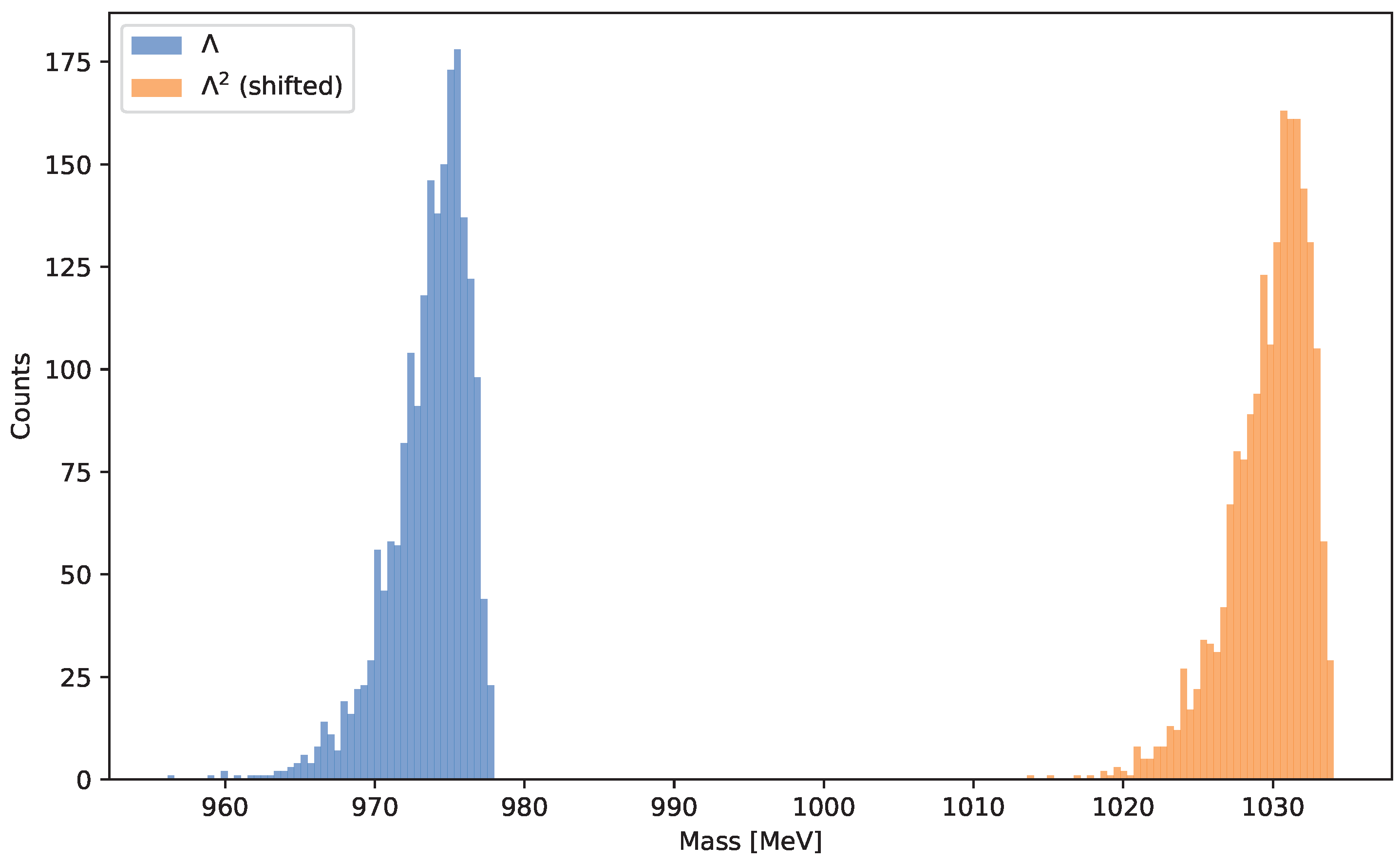
Table 1.
Prime assignments for the baryons.
| Baryon | pattern | -pattern | prime triple | ID in Equation (3.4) |
|---|---|---|---|---|
| p (proton) | ||||
| n (neutron) | ||||
Table 2.
Light baryon masses: model vs. PDG [11]. Residuals ; entries with are coloured red.
Table 2.
Light baryon masses: model vs. PDG [11]. Residuals ; entries with are coloured red.
| Baryon | prime triple | Model [MeV] | PDG 2024 [MeV] | |
|---|---|---|---|---|
| p | ||||
| n | ||||
| 1232 | ||||
| 1232 | ||||
| 1232 | ||||
| 1232 |
Disclaimer/Publisher’s Note: The statements, opinions and data contained in all publications are solely those of the individual author(s) and contributor(s) and not of MDPI and/or the editor(s). MDPI and/or the editor(s) disclaim responsibility for any injury to people or property resulting from any ideas, methods, instructions or products referred to in the content. |
© 2025 by the authors. Licensee MDPI, Basel, Switzerland. This article is an open access article distributed under the terms and conditions of the Creative Commons Attribution (CC BY) license (http://creativecommons.org/licenses/by/4.0/).
Copyright: This open access article is published under a Creative Commons CC BY 4.0 license, which permit the free download, distribution, and reuse, provided that the author and preprint are cited in any reuse.


