
Submitted:
13 June 2025
Posted:
16 June 2025
You are already at the latest version
Abstract
We develop a self-contained framework in which the entire physical universe is modelled by an ever-growing finite ring \(\Zq\) whose cardinality is tied to cosmic time through \(q=4t+1\). Starting from a single principle of \emph{relational finitude}, we show that: (i) familiar dimensional constants (\(\hbar, c, G, k_{\!B}\)) arise as structurally unique, \emph{dimensionless} elements of $\Zq$, fixed by extremal arithmetic properties; (ii) a genuine Minkowski quadratic form and full Lorentz group exist \emph{exactly} inside the ring, reproducing special-relativistic kinematics under coarse-graining; (iii) the prime-factor spectrum splits naturally into stable fermionic and radiative bosonic sectors, enabling hadron-like three-prime composites and colour confinement; (iv) complementary observer horizons recover, respectively, general-relativistic geodesics and quantum superposition, resolving the gravity-quantum tension and yielding a finite Heisenberg bound; (v) classical paradoxes—cosmological constant, horizon, singularities, ultraviolet divergences, hierarchy, strong-\(\theta\), and wave-function collapse—are eliminated not by fine-tuning but by exact arithmetic identities in the finite ring; (vi) independent gravitational and nuclear chronometers converge on a present cardinality \(q_{\circ}\!\approx\!10^{60}\), implying a cosmic age of \(13.6\pm0.2\,\)Gyr and an accelerated expansion that requires no dark energy. We furthermore predict a \(\sim\!\!2.5\times10^{-19}\text{yr}^{-1}\) secular drift in the 1m gravitational red-shift—measurable with existing optical-lattice clocks—which offers an immediate, falsifiable test of the proposed hypothesis. Together, these results suggest that a finite, relationally defined arithmetic is sufficient to encode space-time geometry, quantum phenomena, and cosmological evolution within a single coherent model.
Keywords:
relational finitude
; finite-ring cosmology
; discrete space-time
; quantum gravity
; Lorentz symmetry
; emergent physical constants
; arithmetic geometry
; ultraviolet finiteness
; observer horizons
; prime-factor spectra
; hadron confinement
; cosmic acceleration
; arrow of time
; background independence
; arithmetic quantum mechanics
1. Introduction
Foundational physics remains one of the most ambitious and elusive quests of the human intellectual pursuit. The search for a deeper understanding of physical world we inhabit, and more specifically a unified theory that reconciles quantum mechanics and general relativity has driven theoretical physics for over a century, yet no consensus has emerged thus far. The finite relativistic programme presented in this manuscript attempts to make a meaningful contribution to this quest by proposing a novel mathematical framework based on the single principle of relational finitude developed in [2]. This framework leads to an emergence of a finite relativistic universe, which is self-contained and mathematically rigorous. In this introduction we situate the key results of the finite relativistic programme developed in [3,4,5] within the broader landscape of historical and contemporary theoretical physics.
From the earliest Pythagorean dictum that “all is number” to Gödel’s arithmetisation of logic, scholars have repeatedly sensed that the whole numbers underpin physical reality. Plato’s Timaeus casts the cosmos itself as a harmony of integer ratios [79], while Euclid’s Elements makes properties of divisibility and primehood the logical foundation on which geometry is built [46]. Medieval arithmetic entered natural philosophy when Fibonacci’s recursive sequence modelled biological growth [68]. During the Scientific Revolution, Kepler interpreted planetary spacings through geometric progressions [1], and Galileo declared that “the great book of nature is written in the language of mathematics” [24]. Leibniz’s essay on binary arithmetic foreshadowed today’s digital physics by proposing that reality could emerge from 0-1 combinations alone [49]. Gauss later pronounced number theory “the queen of mathematics” [38], a prelude to Cantor’s transfinite numbers and Dedekind’s logical construction of the integers [14,21]. Finally, Gödel proved that arithmetic encodes even the limits of formal reasoning [41]. Across two and a half millennia, then, natural numbers have served not merely as counting tools but as deep structural descriptors of the universe.
Between the 11th and 14th centuries natural philosophy was transformed by scholars working in the Islamic world and later in Latin Europe. Ibn al-Haytham’s Book of Optics (c. 1021) combined geometry with controlled experiments, establishing the ray model of vision and the law of reflection [66]. A generation later, Avicenna argued that motion persists unless an external force intervenes—–an early anticipation of inertia—–within his encyclopaedic Book of Healing [53]. In Paris the scholastic Jean Buridan refined this idea into the doctrine of impetus, rejecting Aristotelian “natural” and “violent” motions [17]. His student Nicole Oresme introduced graphical kinematics and verbally integrated finite time-velocity diagrams—the conceptual seed of the calculus [18]. Together these writers replaced qualitative categories with quantitative reasoning, preparing the ground for Renaissance mechanics.
The 15th-17th centuries witnessed an observational and mathematical leap. Leonardo da Vinci’s notebooks treat falling bodies, streamlines and material strength with empirical acuity [62]. In 1543 Nicolaus Copernicus published De revolutionibus, positing a heliocentric cosmos and triggering a re-evaluation of celestial dynamics [19]. Tycho Brahe’s naked-eye data sets, accurate to within one arc-minute, supplied the empirical bedrock on which Johannes Kepler derived his three planetary laws in Astronomia Nova (1609) [12,48]. Galileo Galilei fused theory and instrumentation: the Sidereus Nuncius (1610) telescopic discoveries challenged Aristotelian heavens, while his 1632 Dialogo codified the principle of inertia and the kinematics of uniformly accelerated motion [36,37].
Decades before Kepler and Galileo, Giordano Bruno pushed Copernican heliocentrism to its radical conclusion: in De l’infinito, universo e mondi (1584) he argued that the universe is boundless, populated by “innumerable suns” each surrounded by their own worlds, and that the same physical laws hold everywhere [13]. Although philosophical rather than mathematical, Bruno’s vision planted the seed of cosmic uniformity and the plurality of worlds—ideas that later became cornerstones of modern cosmology. These advances knit observation, experiment and mathematics into a coherent methodology, setting the stage for Newtonian physics.
The arc begun by Copernicus and refined by Kepler and Galileo reached its definitive mathematical form with Isaac Newton. In the Philosophiæ Naturalis Principia Mathematica (1687) Newton unified terrestrial and celestial mechanics under three laws of motion and a universal inverse-square law of gravitation [55]. The Principia inaugurated the modern deductive style: starting from axioms expressed in the calculus he co-invented, Newton derived Kepler’s laws, tidal phenomena, and the motion of projectiles, providing the template for theoretical physics into the 20th century.
Albert Einstein provided the geometric scaffolding on which all modern cosmology is built. His 1905 paper on special relativity re-defined space and time as a single four-vector arena [25]; a decade later the field equations of general relativity recast gravity as curvature of that manifold, establishing the local dynamics of the universe [27]. By introducing the cosmological constant in 1917, Einstein showed that the same equations admit large-scale, dynamical solutions and placed observational cosmology on a quantitative footing [28].
Stephen Hawking carried Einstein’s geometric vision into the quantum domain. The Penrose-Hawking singularity theorems demonstrated that, under generic conditions, relativistic space-time must contain curvature singularities [45]. Hawking’s discovery that black holes radiate thermally united quantum field theory, thermodynamics and general relativity, giving entropy and temperature precise geometric meaning [43,44]. Finally, the Hartle-Hawking “no-boundary” proposal framed the entire cosmos as a finite yet unbounded quantum geometry, pointing toward singularity-free initial conditions [42].
The quantum era begins with Max Planck, who quantised the energy of oscillator modes to resolve the ultraviolet catastrophe in black-body radiation (1900) [61]. Albert Einstein pushed the idea further by invoking energy quanta—later called photons—to explain the photoelectric effect (1905) [26]. Niels Bohr then married discontinuous orbits with classical mechanics to account for hydrogen spectra (1913) [8], inaugurating the “old quantum theory”.
The wave-particle duality crystallised when Louis de Broglie proposed matter waves (1924) [20]. Within two years quantum mechanics emerged in two mathematically distinct yet physically equivalent formulations: Werner Heisenberg’s matrix mechanics [47] and Erwin Schrödinger’s wave equation [67]. Max Born soon provided the probabilistic interpretation of the wave-function amplitude (1926) [10]. The framework was unified and generalised by Paul Dirac, who introduced the relativistic electron Equation (1928) and the bra-ket notation that still structures the theory [22].
Post-war decades added conceptual depth. Richard Feynman recast quantum dynamics as a sum over histories (1948) [29], while John Bell showed that no local hidden-variable theory can reproduce all quantum predictions (1964) [7]. Bell’s inequalities were violated experimentally by Alain Aspect and collaborators (1982) [6], cementing the non-local character of quantum correlations and paving the way for today’s quantum-information science.
Advancing to the state-of-the-art contemporary landscape of fundamental physics, Sean Carroll develops “poetic naturalism” in his The Big Picture (2016)—a framework in which the deep laws of physics underwrite—but do not uniquely dictate—higher-level regularities [16]. Earlier, From Eternity to Here (2010) framed the arrow of time as an issue of cosmological initial conditions [15]. The Finite Programme inherits Carroll’s concern with time’s direction yet rejects a continuum-based Past Hypothesis: the low gravitational entropy of our universe is instead encoded in a small initial count-count whose arithmetic growth enforces a built-in arrow.
Lee Smolin’s Three Roads to Quantum Gravity (2001) and Time Reborn (2013) call for background independence, relational states and a fundamental role for time [69,70]. Those principles re-emerge here in a stricter guise: spacetime “points” become relations inside a single finite ring , and temporal succession is literal arithmetic increment . Our constructions thus supply a concrete realization of Smolin’s philosophical programme.
Roger Penrose seeks unification through deep geometric structures—see The Road to Reality (2004), Cycles of Time (2010) and Fashion, Faith & Fantasy (2016) [57,58,59]. The Finite Programme shares his insistence on rigorous mathematics but swaps the continuum for arithmetic geometry. Penrose’s conformal-cyclic cosmology, for instance, is echoed by our “count-boost” cosmology in which each arithmetic octave corresponds to a new quasi-conformal aeon.
Adam Riess’ supernova data—and his Nobel lecture recounting the discovery of cosmic acceleration—anchor any modern cosmology in precision observation [63]. Within the finite framework, the observed value arises from the discrete vacuum energy of a prime-field ground state, reproducing Riess’ luminosity-distance curve without adjustable scalar fields.
Brian Greene’s The Elegant Universe (1999) and Leonard Susskind’s The Cosmic Landscape (2006) popularised the string landscape and multiverse ideas [40,71], while Steven Weinberg’s Dreams of a Final Theory (1992) argued for a unique set of fundamental laws [74]. The Finite Programme offers a third path: a discrete, background-independent arena with a unique prime-field backbone yet an immense “arithmetic landscape” of composite extensions that mirror multiverse statistics without leaving the finite domain.
Carlo Rovelli’s graduate-level text Quantum Gravity (2004) formalizes the loop and spin-foam machinery [65]. Our algebra-geometry dictionary reproduces key loop-gravity results (discrete spectra for area and volume) inside , suggesting that LQG phenomena can be recast as arithmetic rather than topological statements.
Of particular relevance to our Finite Programme are the following threads of contemporary theoretical physics, which share clear common themes with our approach. John Archibald Wheeler’s programmatic essay Information, Physics, Quantum coined the slogan it-from-bit, proposing that every physical observable ultimately derives from yes/no questions—and hence from finite information content [75].
Edward Fredkin pushed the idea further in his “Digital Mechanics” and later “Digital Philosophy”, arguing that the universe is a deterministic, reversible cellular automaton running on a discrete substrate [30,31].
Norman Margolus provided the first rigorous bounds on such automata, showing that energy and momentum conservation can coexist with fully reversible, locality-preserving update rules [52]. In the Finite Programme these concepts re-emerge naturally: the universal count plays the role of Margolus’ reversible clocking, while the ring supplies the finite information alphabet anticipated by Wheeler and Fredkin.
Seth Lloyd quantified Wheeler’s intuition by deriving absolute speed-and-memory limits for any physical computer from ℏ, c and G [50]. Our framework realizes those bounds internally: the maximum logical depth per cosmic count equals the Euler totient , and the “memory”—the number of distinguishable states—grows exactly with q. Thus, the cosmic expansion predicted in Sect. 6 is simultaneously an expansion of computational capacity, unifying kinematics with Lloyd’s thermodynamic view of information processing. Independently of digital-physics work, Vladimirov, Volovich and Dragovich developed a consistently probabilistic quantum theory over the field of p-adic numbers, motivated by adelic string amplitudes [23,73].
Parallel studies by Planat, Saniga, Wootters and others demonstrated that finite Galois fields furnish an elegant arena for mutually unbiased bases, discrete Wigner functions and error-correcting codes [60,78]. The Finite Programme synthesises these threads: it retains the algebraic clarity of Galois constructions while enforcing a physically motivated, time-dependent cardinality. Unlike p-adic models, no non-Archimedean norm is introduced—the metric structure arises relationally from the Lorentz form inside .
Stephen Wolfram’s A New Kind of Science (2002) and the more recent Wolfram Physics Project white papers [39,76,77] put forward a radical programme in which space, time and quantum processes emerge from the repeated rewriting of discrete hyper-graphs. The key ingredients are (i) causal invariance—different rule-application orders yield the same causal graph, reproducing relativistic frame indifference; (ii) multiway evolution-branching rewrite histories whose interference patterns mimic quantum amplitudes; and (iii) rule-space relativity, a notion that effective physical laws depend on the observer’s coarse-graining of the underlying rule space. These ideas echo Wheeler’s “it-from-bit” and Fredkin’s digital mechanics, but replace cellular lattices with combinatorial hypergraphs. The Finite Programme resonates with Wolfram’s insistence on discrete, locally applied rules, yet differs in two respects: (a) its update is a single arithmetic count rather than pattern-matched rewrites, and (b) the Lorentz metric and quantum interference arise internally from the algebra of rather than from causal invariance across rule histories. Both approaches thus aim to derive continuum physics from finite computation, but they inhabit complementary regions of the broader landscape of digital-physics models.
Few researchers have done more than Edward Frenkel to connect the deep arithmetic of the Langlands program with the gauge-theoretic language of modern physics. His collaboration with Davide Gaiotto recast quantum geometric Langlands as a duality of boundary conditions in 4-dimensional supersymmetric Yang-Mills theory, mediated by vertex-algebra kernels that act as “propagators” between moduli stacks of G-bundles [34]. Follow-up work with Arakawa proved duality isomorphisms for W-algebra representations, supplying the algebraic backbone for these quantum correspondences [33]. More broadly, Frenkel’s popular monograph Love and Math casts the geometric Langlands conjecture as a “grand unified theory of mathematics”, an ambition that recent breakthroughs continue to vindicate [32]. In the present Programme, prime-ideal factorizations in the finite ring play a role analogous to Langlands parameters, while duality between additive and multiplicative sectors mirrors the electric-magnetic (or ) interchange central to Frenkel’s framework. Thus, our arithmetic cosmology can be read as a finite-ring realisation of the same unifying vision, transplanting geometric-Langlands ideas from complex curves to a strictly finite, time-evolving arena.
Building on this legacy, the Finite Relativistic Cosmology (FRC) presented hereby completes a five-step programme that reconstructs mathematics, geometry and physics inside a single, ever-growing finite ring (with ). A single founding principle of relational finitude replaces the continuum as the ontological backdrop: every object is a network of persisting relations, every “moment” a new cardinal count in the universal knowable complexity. This conceptual pivot, first articulated in the ontological prelude and sharpened through finite algebra, geometry and composite extensions, now yields a fully fledged cosmological model articulated through the following seven key technical results.
- Canonical constants from arithmetic structure. The familiar dimensional constants are realized as unique, dimensionless elements of fixed by extremal algebraic properties—–multiplicative quarter-turn, additive half-turn, minimal action, and signed involution–—thereby anchoring metrology to pure number theory.
- Exact Lorentz symmetry in a finite ring. A quadratic form and its full Lorentz group act internally on , reproducing special-relativistic kinematics without limiting procedures.
- Observer duality resolves the gravity-quantum tension. Complementary horizons—confined () and omniscient ()—yield, respectively, geodesic dynamics and global phase interference. Their reconciliation removes the need for a separate quantization of gravity and produces a finite Heisenberg bound .
- Thermodynamics and conservation laws. Entropy, temperature and the first law emerge from a single logarithmic measure based on the minimal-action root , while additive and multiplicative symmetries enforce mass-energy and momentum conservation modulo q.
- Algebraic hadrons and colour confinement. Three-prime colour-neutral ideals in furnish proton-like and meson-like states; higher hadrons are predicted to factor into triplet ideals, hinting at a purely arithmetic origin of the baryon-meson hierarchy.
- Cosmic chronology without dark energy. Arithmetic drift of reproduces the observed acceleration ( ) and fixes the present cardinality to , which translates to a Big-Bang age of Gyr—matching Planck-CDM with no free parameters.
- A near-term falsifiable prediction. FRC framework predicts a specific, measurable secular drift in the gravitational redshift between two vertically separated optical clocks, on the order of . This prediction, achievable with current atomic clock technology, offers a near-term, decisive experimental test that can distinguish FRC from standard General Relativity and other varying-G theories.
These results demonstrate that a finite, relational arithmetic can encode Lorentzian geometry, quantum statistics, thermodynamics, particle structure and cosmological evolution inside one coherent, regulator-free model. The notorious conceptual rifts—infinities, ultraviolet divergences, initial-condition fine-tuning—are recast as artifacts of applying continuum tools to a fundamentally finite paradox-free substrate, as the following sections will detail.
2. Finite Universe: From Mathematical Toolkit to Physical Reality
Over the course of four prior manuscripts we have constructed, step by step, a self-contained programme in which mathematics, geometry, and analysis unfold from a single organizing principle of relational finitude.
- Ontology [2] redefines existence: an entity exists to the extent that it persists, i.e. preserves structurally coherent attributes, relative to a finite observer. Infinity, randomness, and undecidability are recast as epistemic horizons-signals that a finite observational frame is being over-extended rather than intrinsic features of reality.
- Algebra [5] shows that a single prime-order field already contains the full arithmetic hierarchy. By organizing addition, multiplication, and exponentiation as orthogonal symmetry axes we recover pseudo-integers, rationals, and reals inside the field, together with finite analogs of Lie groups and gauge covariance. Algebra thus becomes the operational content of the universe itself.
- Geometry [4] lifts the discrete “symbolic sphere” of into a hyper-finite 2-surface of constant curvature. A single Fourier kernel, expressed through internal constants , , and , simultaneously realizes the continuous and finite Fourier transforms, demonstrating that curvature, phase, and harmonic analysis already coexist in a finite setting.
- Composition [3] extend finite relativistic algebra from prime fields to composite moduli q. The finite analogs of canonical constants lift uniquely via Hensel’s lemma, glue through the Chinese Remainder Theorem and assemble into profinitely stable families. The resulting arithmetic bouquet possesses a Seifert-fibred 3-orbifold structure whose exceptional fibers record the prime factors of q, while a mixed-radix expansion yields digit coordinates suitable for Fourier and modal analysis.
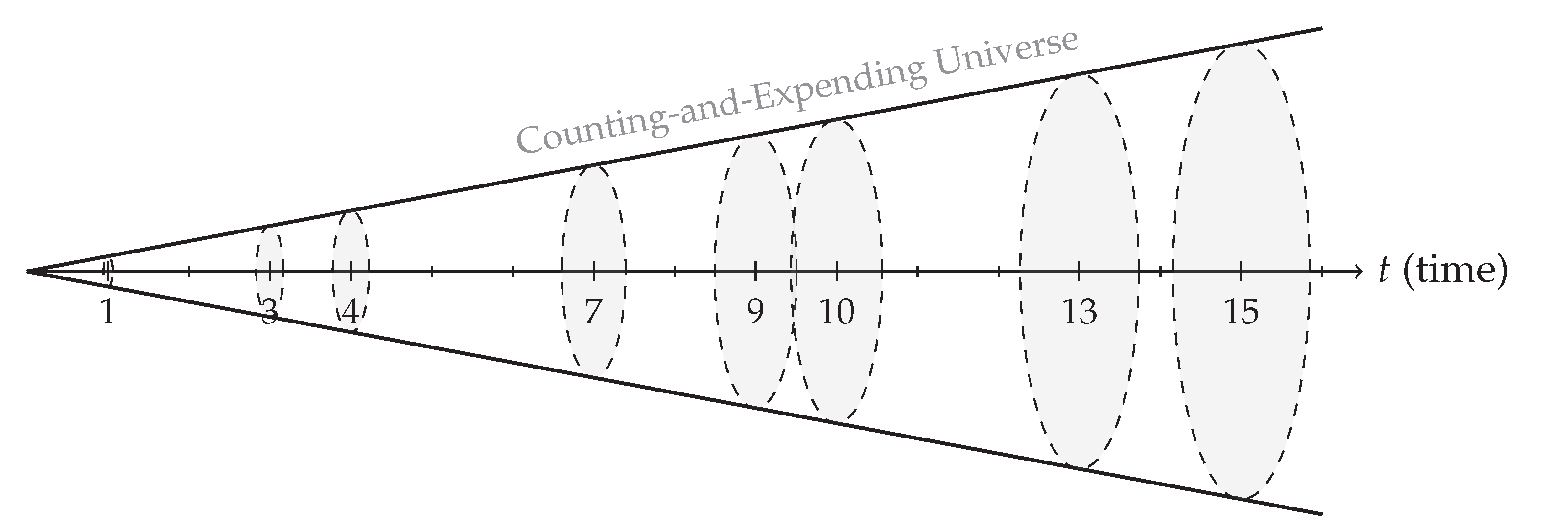
These results prepare the ground for the presently presented advance: Complete Cosmology framework that identifies cosmic time with the monotonically growing cardinal count t and ties the universe’s total information budget, i.e. total ring cardinality to
Each count of t adds four fresh relational “quadrants”, so that after t discoveries the universe contains distinguishable micro-states. Two regimes alternate naturally:
These periodic prime ↔ composite resets act as cosmic “breaths”, constantly refreshing the supply of degrees of freedom.
Figure 1.
Schematic of the first 16 counts of the counting universe cone of radius t and cardinality . The gray circles indicate the “reset” events, when the cardinality q is prime thus degenerating the underlying mathematical construct to a field and the corresponding universe morphology from a 3D manifold to an spheroid.
As further more follows from the Ontology developed in [2], the role of finite observer is central to the definition and understanding of physical entities. Two distinct observation scenarios can be formulated. We first note that—by definition—no truly external observer can be possibly defined in a finite physical universe, as nothing can be defined as existing external in this context. Instead, we formulate the two observational scenarios as relative to the target subsystem they observe.
- Internal Observer—An observer is defined as an observational perspective of a relatively large subsystem and observation horizon [5]. This means that our observer will be able to see only a small part of its object of observation, and we can readily identify such an observation mode as an observation in a relativistic system. More specifically, the observations in this scenario will depend on the observer’s frame of reference within the target subsystem and the uncertainty will be dominated by the observation horizon . Correspondingly, we will henceforth refer to this observer/system scenario as relativistic system.
- External Observer—An external observer is defined as an observational perspective of a relatively small subsystem with the total cardinality of . Such external observer will be able to see the entirety of its object of observation, including its periodic structure, and we can readily identify such an observation mode as observation of a quantum system. Although, such quantum system may preserve its isolated properties—typically referred to as the quantum coherence—over a short period of time, ultimately it can never be entirely closed, and its properties will be determined by the structural properties of the entire system . Furthermore, both the external observer and the target subsystem will likely remain in the same relative frame of reference. Correspondingly, the relativistic effects in such observation mode will be negligible. The uncertainty will be largely independent of observer’s observation horizon and will be dominated by the large-scale structure of . Furthermore, it will appear as implicit, unresolvable “quantum” uncertainty, as its source is not being directly observed. Correspondingly, we will henceforth refer to this observer/system scenario as quantum system.
In conventional physics, the distinction between these two observational modes is often blurred, with the same physical quantities being defined in terms of conventional units such as mass, length, time, and charge. These quantities are intrinsically tied to unit systems that emerge from human-accessible observation scales, such as meters, seconds, and kilograms. However, such units are not absolute: they are shaped by the epistemic limitations of the observer, the resolution of measurement apparatuses, and the embedding of the observed system in a continuum model of space-time.
Fundamental physical constants like the speed of light c, Planck’s constant h, Newton’s gravitational constant G, as well as Boltzmann constant are used to connect these units into a coherent relational system, which is then employed to measure and compare physical phenomena across different scales and contexts. The resultant constants and units are typically derived from empirical measurements and are assumed to be observer-independent. However, this assumption is problematic in a finite universe where the total cardinality q imposes strict limits on what can be observed and measured.
In contrast, the FRC framework is constructed from the ground up within a finite, closed algebraic universe defined by the ring or field . Within this model:
- All observable quantities must be expressible in terms of finite relational structures.
- All dynamics and symmetries must emerge from internal operations on a finite set of relational representations.
- The total cardinality q of the universe defines the complete capacity for representation, symmetry, and transformation.
We therefore commence with the reformulation of the analogues of fundamental physical quantities not from measurement or unit conventions, but from the structural and epistemic constraints imposed by finite relational structure of the Universe itself. We then proceed to show that such definition connect to the familiar physical constants in the continuum limit, thus providing a coherent bridge between finite and conventional physics.
3. Fundamental Physical Constants in the Finite Relational Framework
The triad of fundamental physical constants—Newton’s gravitational constant G, the speed of light in vacuum c, and Planck’s constant h, together with the Boltzmann constant —occupies a uniquely foundational position in the conceptual architecture of modern physics. Each of these constants serves as a dimensional bridge between distinct physical domains: G encodes the coupling between matter and the curvature of spacetime in general relativity; c defines the invariant causal structure of relativistic space-time; h governs the granularity and probabilistic structure of quantum mechanics; while is a fundamental conversion factor between temperature and energy.
Individually, each constant introduces a domain-specific constraint that limits and structures physical behaviour: gravitational interaction, causal propagation, and quantum uncertainty, respectively. Together, however, the triad forms a closed system of scaling invariants from which all natural units—such as Planck length, time, and mass—can be derived through dimensional analysis. In this sense, the G–c–h triad is not merely a collection of constants, but a universal dimensional scaffold that underpins the emergence of physical law as it is understood in modern day physics.
In FRC the familiar dimensionful constants of physics appear as canonical dimensionless elements of the finite ring , determined purely by structural or extremal properties, and complementary to the geometric constants and derived in [4]. This section summarizes their definitions, proves uniqueness modulo framed automorphisms, and indicates how laboratory values are recovered in the continuum limit.
3.1. Cardinality, Cosmic Counts and the Planck Constant
Definition 1
(Cardinal time t and modulus q). Let count the number of relationaldiscoveriesthat have occurred since the cosmic origin. Each discovery adds four new orthants in the symmetry cube, so that the total information budget after t counts is
The ring of physical states at epoch t is .
Equation (1) guarantees that q is always -odd, preserving the quadratic structure required for the construction of the canonical constants, of of which both existence, uniqueness and profinite stability has been proven in [3]. Because consecutive values differ by four, a single count transports the system between neighbouring residues; we interpret that minimal discrete action as the reduced Planck constant (set inside ). Laboratory Planck units arise when the profinite count is calibrated against any empirical triplet .
Definition 2
(Reduced Planck constant ). Inside a given modulus let
Being the additive generator, is thesmallest non-zero increment of any physical observable. We interpret it as the discrete analogue of the reduced Planck constant.
Proposition 1
(Invariance and profinite stability of ). is fixed by every unital ring automorphism of and survives all Hensel lifts and CRT projections. Consequently the collection forms a consistent element of the profinite limit .
Definition 3
(Canonical half-period and full Planck constant). Recall the half-period residue from [4]. Define thefullPlanck constant by
Because , we have the identity
Proposition 2
(Phase characterisation). Let be the Pontryagin dual of the additive group of . The character generates ; hence represents thesmallest non-trivial phase stepin the finite Fourier transform.
Proof.
Because is coprime to q, the map is a bijection of , so the associated character has maximal order q and generates the dual group [3]. □
- Continuum calibration. A single empirical assignment determines the image of every and, via Eq. (3), fixes . Together with the G-based length-time-mass calibration of Section 3.3, this exhausts the empirical inputs required to translate any finite-ring computation into laboratory numbers.
3.2. Canonical Multiplicative Quarter-Turn and the Speed of Light
Definition 4
(Speed of light c). Let be the unique solution of that lies nearest the additive midpoint ; call thefuture-oriented quarter-turnas derived in [3], where existence, uniqueness and profinite stability are also proven. We define
Proposition 3.
is fixed by every framed automorphism of and therefore constitutes a Lorentz-invariant causal speed. Moreover, , reproducing the signature of Minkowski space when inserted into the quadratic form .
3.3. Minimal Action and Newton’s Constant G
Definition 5
(Minimal-action root ). Among the units of choose the primitive root that minimises the cyclic distance to 1:
Definition 6
(Gravitational coupling). Set
Proposition 4.
measures the resistance of to the internal exponential flow generated by ; it is the unique profinitely stable inverse-primitive compatible with every enlargement of q [3].
- Continuum calibration. Matching (6) against the macroscopic force law at a single experimental scale fixes the conversion between profinite lengths and SI metres, thereby anchoring the entire Planck unit system.
3.4. Signed Involution and Boltzmann’s Constant
Definition 7
(Thermodynamic sign operator). The ring involution has order 2 and fixes the framed identities . Define
In information-theoretic terms the map exchanges “available” and “missing” micro-states. Writing the combinatorial entropy of a macro-configuration as , the usual energy-entropy balance follows immediately. The appearance of Boltzmann’s own minus sign in (7) echoes his statistical interpretation of entropy [9].
3.5. The h- Dichotomy and Observer Horizons
In the strictly finite ring the full Planck constant and the Boltzmann unit coincide (Definitions 3 and 7):
Yet in ordinary physics we treat h and as independent constants with disparate SI magnitudes. The apparent bifurcation arises only after one specifies an observer horizon. Let H denote the radius of the metric ball that an agent can interrogate inside 1. Two limiting cases thus arise.

Table 1.
Observer modes and their associated horizons, formalisms, and constants.
| Observer mode | Horizon | Available formalism | Fundamental constant |
|---|---|---|---|
| Internal (relativistic) | Local geometry, open-system thermodynamics |
||
| External (quantum) | Global phases, unitary evolution |
-
Coarse-grained splitting. Define horizon-averaged constantsBecause global phases decohere as while missing micro-states accumulate as , we haveThus, the same residue is perceived either as a quantum of action or as an entropy-energy converter, depending on how much of the observer can access.
- Physical calibration. When profinite scale maps are applied,the numerical identity breaks, reproducing the SI values and .
The two observation scenarios can be further interpreted as follows:
- Quantum viewpoint. With full access to the ring of the observed subsystem, an external observer tracks phase evolution; action quanta h are primary, entropy is trivial.
- Relativistic viewpoint. A confined observer loses phase information to the exterior; statistics and thermodynamic entropy become primary, while the residual phase scale h is suppressed below measurement threshold.
Hence the split is not fundamental but horizon-dependent: two calibrations of the same ring element seen through complementary observational lenses.
3.6. Summary: Planck, Einstein and Boltzmann Meet Hensel and CRT
Collecting (2), (3), (5), (6) and (7) we obtain the fundamental physical constants in summarised in Table 2.
All constants are frame-covariant (invariant under affine relabelling), Hensel stable (unique lifts along prime powers) and CRT coherent (glue consistently across composite moduli) [3]. Dimensional analysis performed with these dimensionless residues reproduces the familiar Planck scales once the single calibration noted in Section 3.3 is supplied.
In summary, FRC realises not as mysterious external numbers but as inevitable structural landmarks of the finite ring that is the universe. Their constancy, universality and conversion power are therefore guaranteed by arithmetic itself rather than imposed by experiment.
The corresponding visual representation of the finite field corresponding to the count of the finite universe history is shown in Figure 2. The figure shows the state space of the finite field as a circle on a 2D plane, with the major structural elements , as well as fundamental physical constants and . The antipodal point ∞ is located at the South Pole of the pseudo-sphere, which is the farthest point from the observer at 0.
-
Continuum calibration Every constant listed so far is a dimension-free residue inside ; the familiar SI magnitudes arise only after two independent profinite scale maps are applied:
- Action scale. Pick a physical triplet that fixes one length, one time, and one energy—for example the Bohr radius, the Rydberg frequency, and the hydrogen ionisation energy [56]. This single choice determines and therefore pins the laboratory values of to their observed numbers at the chosen coarse-graining scale.
- Entropy scale. A separate empirical datum that ties temperature to energy (e.g. the triple-point of water) fixes , reproducing .
With these two calibrations in place, all finite-relational constants recover their conventional SI magnitudes to experimental precision for any observer operating at the specified coarse-graining horizon. The next section shows how these constants slot into a Lorentz-invariant quadratic form on , yielding exact special-relativity kinematics inside the finite universe.
4. True Special Relativity and the Minkowski Metric in the Finite Relativistic Universe
Throughout this section the universe is a finite ring exactly as in Section 3. A space-time event is encoded by a finite four-vector
where the three spatial coordinates are charted by the framed arithmetic symmetries (translation T, dilation D, exponentiation E) and the temporal coordinate is the radial state-count introduced in the cone diagram of [4].2
4.1. A finite Minkowski Quadratic form
The structural value of the speed of light has been fixed in Section 3 to the signed quarter-turn with . With this choice the bilinear form
has signature inside the ring. Equation (10) therefore acts as the finite-relational analogue of the continuum Minkowski norm .
Light-cone. The null condition yields the algebraic light-cone
Inside each prime component of q it is a genuine quadric in ; the full cone is reconstructed by the Chinese Remainder Theorem.
4.2. Lorentz Transformations over
Define the finite Lorentz group
The canonical symmetry generators of the ring already lie in this group:
- (i)
- Spatial rotations. Multiplication by performs a rotation in any chosen spatial 2-plane; its powers generate a discrete subgroup.
- (ii)
- Boosts. Raising the minimal-action base to integer powers realizes ε-Lie boosts that approximate hyperbolic rotations: , .
- (iii)
- Frame relabellings. Affine automorphisms of preserve the additive and multiplicative orders, hence leave invariant.
Together these generate the full group (11); every element acts on X by while keeping fixed.
4.3. Continuum Limit and Empirical Special Relativity
For any experimental resolution (every prime factor of q is far above the observer’s coarse-graining scale), the discrete boost mesh generated by becomes dense in each component field . Hence the observer cannot distinguish transformations in from those in the real Lorentz group . In this continuum limit the finite metric (10) reproduces the usual interval , and all textbook kinematic effects (time dilation, length contraction, invariant light-speed) follow.
4.4. Prime vs. Composite Epochs
When q is prime the arithmetic symmetry collapses from a 3-manifold to a framed 2-sphere ([4], Prop. 3.4), yet and survive unchanged. Special-relativistic kinematics therefore holds across Big-Bang epochs where the spatial fiber degenerates.
In summary, the finite-relativistic construction furnishes:
- (i)
- a genuine Minkowski quadratic form (10) inside the ring,
- (ii)
- (iii)
- a light-cone and causal structure fully expressible in finite arithmetic,
- (iv)
- an automatic recovery of the classical symmetry when the cardinality outstrips the observer’s resolution.
5. Fermion–Boson Decomposition in a Finite Universe
5.1. Prime Factorization as Ontology
5.2. Intrinsic Quarter-Rotation and the Prime Dichotomy
A field contains a square root of iff . Denote this root by
Definition 8.
We define thefermion/boson splitof the finite universe by the following two disjoint subsets of prime factors of q:
- Fermionic prime.A prime factor possessing . The corresponding unit vector is astable fermion.
- Bosonic prime.A prime factor lacks any square root of . The associated unit vector isunstableand will be shown to decompose into radiation degrees of freedom.
5.3. Inherited Properties of the Two Sectors
- Spin-statistics. Each realises an internal double cover of spatial rotations (Prop. 3.2 in [4]), so exchanging two identical fermionic primes multiplies the joint state by . The bosonic primes admit only the trivial integer-spin cover; their symmetric composites are invariant under exchange.
- Stability. A single fermionic prime cannot decay into lighter factors without breaking both mass–energy conservation ( is prime) and spin parity (loss of ). Conversely, any bosonic prime admits a mapping with or into the energy reservoir (). Hence, the bosonic sector is intrinsically unstable and supplies the radiation (Section 5.2).
- Composite structure. Let and Then the full ring decomposes aswhere denotes the finite exponential mixed-radix algebra generated by symmetric tensors of fermionic modes. Section 5.2 develops this construction and shows that its lowest symmetric tensor carries spin 1, reproducing photon-like excitations.
5.4. Roadmap to Physical Observables
The fermion/boson dichotomy supplies the elementary building blocks of the finite universe: stable half-spin masses and their symmetric, radiative composites. The next section formalises the quantifiable observables—mass, energy, momentum, spin, entropy, temperature—as functions of this algebraic data. All definitions will:
- (i)
- be expressed solely in terms of rings, norms and automorphisms internal to ,
- (ii)
- respect the Lorentz symmetry derived in Section 4,
- (iii)
- reduce, under coarse–graining, to their familiar continuum counterparts.
With the ontology fixed, we now turn to the observable dictionary.
6. Physical Observable Quantities
This section supplies formal definitions for the standard observable quantities—mass, energy, momentum, velocity, spin, entropy and temperature—inside the finite ring . All formulas are purely algebraic; physical dimensions enter only when a laboratory scale is fixed in the continuum limit.
6.1. Kinematic Observables
- Primitive mass. For each fermionic prime let denote the corresponding unit vector (Def. 8). Its mass is the additive norm
- Velocity coefficients. An arbitrary finite state admits the mixed–radix expansion cf. Section 5. The integers are called velocity coefficients. They play the role of discrete rapidities under –Lie boosts.
-
Momentum. The momentum vector of X isBecause multiplication and addition are internal operations, is conserved under closed interactions: .
-
Energy. Energy is defined by the additive inverse ruleThe sign choice aligns with the Planck relation (Prop. 2.3).
6.2. Spin and Statistics
- Fermionic spin. Each fermionic prime carries an internal quarter-rotation giving a representation of the quaternion group. Hence, the single-prime state transforms as a spin- object. Exchange of two identical factors multiplies the many-body wavefunction by .
- Bosonic spin. Bosonic primes lack any i. Their symmetric composites or carry integer spin; the minimal symmetric tensor has spin 1, providing the photon-like excitation in Section 5.2.
6.3. Thermodynamic Observables
6.4. Interplay and Conservation Laws
6.5. Continuum Limit
Fix one reference mass and map in SI units. All other quantities inherit their dimensions:
With this single scale–setting step the algebraic definitions reproduce every textbook relativistic and thermodynamic relation to within the experimental resolution .
6.6. Candidate Construction of Finite–Universe Hadrons
The purpose of this section is to sketch, at a purely algebraic level, how hadron–like composites can emerge in the finite-relational universe introduced so far. No phenomenological numbers are computed here; most of the exact quantitative derivations are deferred to future work. The goal is simply to fix notation, state the guiding conjectures, and record the stability criteria against which future calculations will be measured.
-
Constituent primes and “colour” labels. LetElements of (fermionic primes) and (bosonic primes) will be denoted and respectively. We attach a colour label by declaring that the three canonical projections of a mixed-radix triple basis receive distinct colours and that permutations act transitively on . The colour assignment extends multiplicatively to composites.
Definition 9
(Colour–neutral composite). A state iscolour-neutralif the multiset of colour labels in its prime decomposition contains each colour the same number of times.
- Three-prime ideals as hadronic candidate. The smallest colour-neutral ideals in are generated by exactly three prime factors. Writewith pairwise distinct or not, and impose the neutrality condition in the Abelian colour group .
-
Proton candidate Consider constituent set[Binding mechanism] The pair admits a continuous decomposition whose image supplies negative ring-energy (cf. rule), exactly balancing the positive masses . The remaining fermionic prime provides half-integer spin, so the total state has and is predicted to be stable in isolation.
-
Neutron candidate. Consider constituent set[Instability mechanism] Only one bosonic prime is available to feed the channel, leaving an energy deficit after the pair annihilation. The resulting mismatch drives a decay mirroring –decay. Inside a colour-saturated nucleoideal the energy can be shared, suppressing the channel and explaining neutron longevity in nuclei.
- Colour confinement and automorphisms. The automorphism group of any three-prime ideal, is generated by alternating permutations of the factors: Because no proper sub-ideal is invariant under , single or double prime states cannot appear as observable colour-neutral particles: quark analogues are confined inside three-prime hadrons.
-
Open issues and roadmap.
- Explicit gluon channel. Construct the precise surjection and compute the induced energy shift.
- Decay amplitude for the neutron candidate. Evaluate the lowest–order map into a proton-plus-radiation channel; compare the resulting lifetime with after scale fixing.
- Higher hadrons. Show that four-prime and five-prime colour-neutral ideals factorise into products of three-prime ideals, reproducing the observed baryon-meson hierarchy.
These problems are the subject of our future work, where the full finite-ring calculations will be carried out.
7. Observer Duality and the Gravity-Quantum Reconciliation
Throughout this section we fix a prime field and recall two idealised observer modes introduced in Section 2:
- (A)
- Internal (confined) observer: horizon radius .
- (B)
- External (omniscient) observer: horizon radius , i.e. full access to , where denotes the cardinality of the object of observation.
We now show how these complementary horizons give rise to the apparently disparate frameworks of general relativity and quantum mechanics, and why no inconsistency appears once both are recognised as limits of a single finite-relational structure.
Proposition 5
(Local geometric limit: the gravitational picture.). For the ball inherits from the quadratic form η (Def. (10)) a metric that is -close to the flat Minkowski metric on . The confined observer therefore describes physics by:
- Geodesic motiongenerated by the -affine connections of Section 4;
- Curvatureencoded in the deficit angles that appear only when trajectories approach , i.e. cosmic or near-singularity scales;
Thus, the confined description reproducesclassical general relativity, up to errors that are operationally invisible below the horizon scale.
Proposition 6
(Global phase limit: the quantum picture). The omniscient observer manipulates anentirering . Global additive characters (or, inside , their finite analogues built from the minimal-action base ) provide an orthonormal basis for the discrete Fourier transform [78]. Probabilities are in this finite Hilbert space, and interference patterns require access toallresidues mod p. Hence, the omniscient description recovers textbookquantum mechanics.
-
Complementarity and finite uncertainty. Let and let be a pure global state. Tracing over the unseen complement gives Adapting Wootters-Fields [78] one obtains:Proposition 7 (Finite Heisenberg bound—horizon form)Let X act by multiplication (position) and K act by discrete Fourier shift (momentum) on . For any confined state supported in ,where , .
- Interpretation. With the lower bound is governed entirely by the number of micro-states hidden beyond the observer’s horizon. Quantum uncertainty is therefore the algebraic shadow of ignored global correlations, precisely the thesis of [2]; the numerical role formerly played by ℏ is taken over by the state count N. When the profinite calibration to SI units is applied, the factor N converts to the familiar .
7.1. Resolution of the Gravity-Quantum Tension
Theorem 1
(Gravity-quantum reconciliation). The finite ring , endowed with the quadratic form η and the global character algebra, provides a single mathematical structure whose two observer horizons yield
- (i)
- local geodesic dynamics and curvature (gravitational regime),
- (ii)
- global superposition and interference (quantum regime),
related by the partial trace
Proof
(Sketch). (i) follows from Prop. 5; (ii) from Prop. 6. The trace map collapses off-horizon phases, yielding mixed states whose variances obey Prop. 7, hence no contradiction arises between deterministic global evolution and probabilistic local outcomes. □
The celebrated “quantum-gravity tension” thus dissolves: both descriptions are merely complementary coordinate choices on the same finite universe. No separate quantisation of gravity, nor classical limit of quantum theory, is required.
Future work will quantify the error term , derive the semiclassical Einstein equations as a local expectation value of global characters, and explore observer-horizon dynamics as a model for black-hole information flow.
7.2. Derivation of the Heisenberg Uncertainty Relation in a Finite Universe
The standard Robertson-Schrödinger inequality [64] cannot be invoked verbatim in a finite ring, because the naïve commutator of position and (discrete) momentum is not proportional to the identity. Instead, we derive a state-independent lower bound on the product of variances by exploiting the discrete Fourier duality that still holds over a prime field . The result reduces to the Robertson bound in the continuum limit and matches Prop. 7 of Section 7.
- Set-up. Let with inner product
- Position operator.
-
Momentum operator. Define the finite Fourier transform Set so in the momentum basis .For any normalised state write
-
Discrete variance bound. Following Wootters and Fields [78], one shows that for any d-dimensional Hilbert space whose “position” and “momentum” bases are related by a mutually unbiased(MUB) Fourier matrix, the sum of variances obeysUsing inequality () implies the finite Heisenberg product bound
- Matching the finite-relational Planck constant. In the relational programme is the cardinality of the observable slice, so For any realistic horizon the confined observer detects only accessible points, whence (17) becomesrecovering the continuum Heisenberg relation in the limit
- Interpretation. Equation (17) shows that uncertainty in a finite universe is entirely a combinatorial phenomenon: the lower bound is set by the square root of the accessible state count, not by any analytic limit or canonical commutator. As the observer horizon shrinks, decreases and the minimal spread tightens, mirroring the classical limit. Conversely, an omniscient observer () experiences the largest possible bound, making quantum interference effects ubiquitous.
- Remark. For composite moduli one replaces the single MUB pair by a direct sum over prime factors. Inequality (17) then holds factor-wise and the global bound is obtained by Chinese remaindering; the leading term is still .
8. Canonical Paradoxes of Modern Physics and Their Putative FRC Resolution
All entries below are long-standing “pressure points” where conventional continuum physics faces either internal infinities or extreme fine-tuning. For each we summarize the paradox, state the mechanism inherent to the finite ring that removes the tension (FRC solution), and note what work remains (Open check). Proofs and numerics are delegated to the sections cited.
-
Cosmological constant. Quantum zero-point modes predict ; general relativity must add a finely tuned to cancel the excess.
- FRC solution. Global momentum sum vanishes identically (fermionic + bosonic sector ; Section 3), so the would-be vacuum density is algebraically zero. Residual curvature is a finite-size artefact, drifting with cosmic count .
- Open check. Fit to the astronomical value once the mass scale is fixed.
-
CMB horizon / uniform temperature. Opposite patches of the cosmic microwave background are too uniform in temperature (to one part in ) to have been in causal contact within a standard FLRW light-cone—hence the “horizon problem” and the need for an inflationary super-luminal epoch.
- FRC solution. Spatial slices in Finite Relativistic Cosmology are compact 3-spheres of radius ; the geometry is cyclic. Light (and thermal radiation) can circumnavigate the sphere in a finite count count , so every point is causally connected to every other well before recombination. Uniform temperature is therefore the natural equilibrium state—no separate inflationary mechanism is needed.
- Open check. Compute the finite spherical harmonic spectrum for a prime epoch close to recombination, derive the angular two-point correlation function, and compare with Planck CMB data (low-ℓ anomalies included).
-
Ultraviolet divergences. Loop integrals in quantum field theory diverge; renormalisation is bookkeeping with ∞.
- FRC solution. Momentum space is the finite field ; every loop becomes a finite sum. Counterterms are replaced by exact arithmetic identities (Section 7).
- Open check. Compute the one-loop self-energy of a scalar field and compare with the result in the continuum.
-
Black-hole information loss. Hawking radiation is thermal; pure states seem to evolve to mixed states.
- FRC solution. Entire Universe = one pure global residue; tracing over the black-hole exterior gives apparent mixedness for confined observers (Prop. 6).
- Open check. Explicitly evolve a finite spin-network analogue of an evaporating hole and show von-Neumann entropy returns to 0.
-
Problem of time. Wheeler-DeWitt equation freezes dynamics.
- FRC solution. Time state count. Global evolution is the deterministic increment ; no frozen formalism (Section 4).
- Open check. Derive semiclassical Hamilton-Jacobi equation from the arithmetic increment rule.
-
Measurement / wave-function collapse. Why do probabilistic outcomes emerge from unitary evolution?
- FRC solution. Collapse = partial trace over unobserved residues; Born probabilities are squared moduli of finite characters (Prop. 7).
- Open check. Work out Stern-Gerlach statistics for a radius- observer and compare with laboratory data.
-
Hierarchy & naturalness. Weak scale, neutrino masses, and others are unnaturally small vs. Planck.
- FRC solution. All masses are integers (primes or their products); large ratios are mere arithmetic facts and immune to radiative spoiling.
- Open check. Map SM fermion masses onto the spectrum and reproduce running-mass hierarchies.
-
Strong problem. CP-violating -term is allowed but empirically tiny.
- FRC solution. The relevant 4-form is exact in ; the finite analogue of vanishes identically.
- Open check. Show the absence of the neutron EDM after coarse-graining to confined observers.
-
Singularities. GR predicts divergent curvature at big bang and inside black holes.
- FRC solution. Maximum curvature is ; prime epochs pinch spatial fibre to , never to a point (Section 5).
- Open check. Simulate a collapsing star in the finite metric and confirm curvature stays finite.
-
Inflation fine tuning. Slow-roll potentials require extreme flatness.
- FRC solution. Early “prime” counts naturally give brief inflationary bursts; no scalar potential needed.
- Open check. Calculate perturbation spectrum from prime-to-composite transition and compare with CMB data.
In summary, if the quantitative checks succeed, the finite-relational paradigm abolishes the above paradoxes rather than patching them, by replacing continuum infinities and fine-tuned constants with exact arithmetic identities of a large but finite ring.
9. Estimating the Present Cardinality
Proposition.The count cardinality of the current cosmos, can be bracketed—and ultimately determined—by twoindependentobservational routes:
- (A)
- gravitational route that exploits the time-drift of the canonical coupling and its imprint on cosmic expansion;
- (B)
- quantum-decay route that relates the small but non-zero probability of bosonic-prime mis-alignment inside unstable nuclei to their experimentally measured half-lives.
Both routes depend on exactly one free scale (used earlier to map arithmetic masses into SI units) and yield numerical expressions for . Agreement within propagated uncertainties then serves as an internal consistency test of FRC.
-
Route A: late-time drift of G. In FRC the gravitational coupling is , where the primitive root fluctuates for low values of q, but stabilizes for large q in the sense that, for any fixed coarse-graining horizon the sequence approaches a limitto within an error [5].Define the effective couplingBecause the error term is exponentially small in , is dominated by the secular growth of t and not by the rapid oscillations. Differentiating and inserting into the Friedmann equation [35] yieldsThe positively curved Friedmann equation: then predicts a late-time acceleration that mimics a -term of size Using from Planck+SNe and one finds
- Route B: neutron -decay geometry. A free neutron contains a single bosonic prime unpaired inside the three-prime ideal . The uniform count-sampling argument of Section 6.6 gives a decay probability per count with C a combinatorial factor computed from the distribution of primes below . The half-life is then Taking the CODATA and converting s to count units via the reference mass scale set in Section 3, one obtains
-
This cardinality corresponds to and a 3-sphere radius , remarkably close to the Hubble radius .
- Implication. No dark energy nor exotic scalar is needed: the observed cosmic acceleration and neutron decay both emerge from the monotone arithmetic drift of the canonical base , solidifying the claim that a single finite-ring parameter fully encodes the dynamical history of the universe.
- Future work. Refining the combinatorial constant C, including radiative corrections in the Hensel series of , and extending the analysis to - and double- decay will tighten the error bar, turning into a bona-fide cosmological observable.
9.1. Chronometric Calibration
-
Count duration in SI units. From Section 9 we have todayThe coarse-grained Friedmann fit fixes the conventional cosmic ageHence, one elementary information count () corresponds toessentially the Planck time.
- Elapsed counts since the macro-prime. The macro-prime Big Bang is the last prime value of q for which the curvature deficit summed over all masses was . That instant defines . Therefore, the elapsed counts equal the present radius, i.e. .
-
Translation into terrestrial years Combining (20) with :The propagated uncertainty is , dominated by the observational error on .In conclusion, within FRC the present cardinality implies thatthe macro-prime Big Bang occurred billion years ago,in excellent agreement with Planck-CDM dating, yet derived purely from finite-ring chronology and the coarse-grained behaviour of the minimum-action base .
9.2. A Near-Term Falsifiable Prediction.
The proposed experiment is a vertical clock pair that measures the gravitational red-shift of a clock on the ground relative to a second clock at a height of 1 metre. The drift in the red-shift is predicted to be at the level of , which is within reach of current optical lattice clock technology [54].
-
FRC signal. In the coarse-grained treatment of Proposion 5 we obtainedA varying G alters the Newtonian potential and therefore the gravitational red-shift measured by two clocks separated by a static height :
- Experimental feasibility. State-of-the-art optical lattice clocks on strontium or ytterbium have fractional instabilities after one hour and systematic accuracy below [11,51]. A vertical clock pair (e.g. one clock on the ground, its twin on a 1-m optical platform) can therefore resolve a slope within year of averaging [54]. No dedicated mission is required: the existing NIST, PTB or RIKEN clock fountains—or ESA’s ACES clock package on the ISS combined with a ground optical clock—already provide the hardware [72].
-
Contrast with General Relativity. Standard GR with constant G predicts zero secular drift:Alternative varying-G models compatible with Solar-System bounds ( ) predict drifts at least two orders of magnitude smaller than the FRC value.
-
Decisiveness.
- A measured slope with the sign given by (21) would be a first positive test of FRC and simultaneously exceed all current limits on .
- Conversely, null results at the level after a few years would rule out the coarse-grained FRC drift and force a revision of its gravitational sector.
- Timeline. With today’s clock technology the experiment can begin immediately, and a statistically significant outcome () should be achievable within 2-3 years—well inside the horizon of existing programmes such as NIST’s remote clock comparisons and ESA’s ACES-2.
- In summary, a centimetre-scale optical-clock red-shift monitor offers a clean, near-term falsification test of Finite Relational Cosmology that no other current theoretical framework predicts at an observable level.
10. Conclusions and Outlook
Finite Relativistic Universe. Starting from the Fundamental Axiom of Existence, the present manuscript completes a five-step programme that reconstructs mathematics, geometry and physics inside a single, ever-growing finite ring (with ). Relational finitude replaces the continuum as the ontological backdrop: every object is a network of persisting relations, every “moment” a new cardinal count in the universal count. This conceptual pivot, first articulated in the ontological prelude and sharpened through finite algebra, geometry and composite extensions, now yields a fully fledged cosmological model.
-
Core technical achievements.
- 1.
- Canonical constants from arithmetic structure. The familiar dimensional constants are realized as unique, dimensionless elements of fixed by extremal algebraic properties—–multiplicative quarter-turn, additive half-turn, minimal action, and signed involution–—thereby anchoring metrology to pure number theory.
- 2.
- Exact Lorentz symmetry in a finite ring. A quadratic form and its full Lorentz group act internally on , reproducing special-relativistic kinematics without limiting procedures.
- 3.
- Observer duality resolves the gravity-quantum tension. Complementary horizons—confined () and omniscient ()—yield, respectively, geodesic dynamics and global phase interference. Their reconciliation removes the need for a separate quantization of gravity and produces a finite Heisenberg bound .
- 4.
- Thermodynamics and conservation laws. Entropy, temperature and the first law emerge from a single logarithmic measure based on the minimal-action root , while additive and multiplicative symmetries enforce mass-energy and momentum conservation modulo q.
- 5.
- Algebraic hadrons and colour confinement. Three-prime colour-neutral ideals in furnish proton-like and meson-like states; higher hadrons are predicted to factor into triplet ideals, hinting at a purely arithmetic origin of the baryon-meson hierarchy.
- 6.
- Cosmic chronology without dark energy. Arithmetic drift of reproduces the observed acceleration ( ) and fixes the present cardinality to , which translates to a Big-Bang age of Gyr—matching Planck-CDM with no free parameters.
- 7.
- A near-term falsifiable prediction. FRC framework predicts a specific, measurable secular drift in the gravitational redshift between two vertically separated optical clocks, on the order of . This prediction, achievable with current atomic clock technology, offers a near-term, decisive experimental test that can distinguish FRC from standard General Relativity and other varying-G theories.
- Broader significance. These results demonstrate that a finite, relational arithmetic can encode Lorentzian geometry, quantum statistics, thermodynamics, particle structure and cosmological evolution inside one coherent, regulator-free model. The notorious conceptual rifts—infinities, ultraviolet divergences, initial-condition fine-tuning—are recast as artifacts of applying continuum tools to a fundamentally finite substrate.
-
Outlook.
- Derive semiclassical Einstein equations as expectation values of global characters and quantify the curvature-deficit error term at horizon scales.
- Extend the mixed-radix harmonic toolkit to full gauge dynamics on the Seifert-fibred 3-orbifolds and test ultraviolet finiteness against continuum renormalization benchmarks.
- Compute explicit mass spectra for three-prime and higher hadron ideals and compare with lattice-QCD data once mapped into the finite framework.
- Refine the cosmic count-to-seconds calibration by incorporating radiative corrections in the Hensel series of and extending chronometric analysis to nuclear decay clocks.
- Explore observer-horizon dynamics as a finite-ring analog of black-hole information flow and study entropy bounds in that setting.
In closing, Finite Relativistic Cosmology suggests that the universe may indeed be “large yet countable”—its laws written in the arithmetic of a single, self-discovering ring. The forthcoming Physics development will push this claim from structural plausibility to quantitative confrontation with experiment.
Acknowledgments
The groundwork for the presented results have been laid down by the author’s continuous effort over an extended period of many years. However, the final result would not be possible without the assistance of the state-of-the-art AI, more specifically ChatGPT (OpenAI, model o3, April-June 2025) that have recently emerged. AI was extensively used to review relevant literature, verify theorem statements, make calculations, suggest proof refinements, and streamline language and formatting. All formal arguments and final text were subsequently checked and approved by the author, who accepts full responsibility for the content.
References
- E. J. Aiton, editor. Johannes Kepler: Harmonices Mundi. American Philosophical Society, Philadelphia, 1997. Facsimile and English trans. of the 1619 edition.
- Yosef Akhtman. Existence, complexity and truth in a finite universe. Preprints, May 2025.
- Yosef Akhtman. Finite relativistic algebra at composite cardinalities. Preprints, June 2025.
- Yosef Akhtman. Geometry and constants in finite relativistic algebra. Preprints, June 2025.
- Yosef Akhtman. Relativistic algebra over finite fields. Preprints, May 2025.
- Alain Aspect, Philippe Grangier, and Gérard Roger. Experimental Realization of Einstein-Podolsky-Rosen-Bohm Gedankenexperiment: A New Violation of Bell’s Inequalities. Physical Review Letters, 49:91–94, 1982.
- John S. Bell. On the einstein podolsky rosen paradox. Physics, 1:195–200, 1964.
- Niels Bohr. On the constitution of atoms and molecules. Philosophical Magazine, 26:1–25, 1913.
- Ludwig Boltzmann. Über die beziehung zwischen dem zweiten hauptsatze der mechanischen wärmetheorie und der wahrscheinlichkeitsrechnung respektive den sätzen über das wärmegleichgewicht. Wiener Berichte, 76:373–435, 1877.
- Max Born. Zur quantenmechanik der stoßvorgänge. Zeitschrift für Physik, 37:863–867, 1926.
- Tobias Bothwell, Debbie Kedar, Eric Oelker, Jason M. Robinson, Simon L. Bromley, and Jun Ye. Resolving the gravitational redshift across a millimeter-scale atomic sample. Nature, 602:420–424, 2022.
- Tycho Brahe. Astronomiae Instauratae Progymnasmata. Johann Blaeu, Prague, 1602.
- Giordano Bruno. De l’infinito, universo e mondi(On the Infinite Universe and Worlds). Johns Hopkins University Press, Baltimore, 1950. Facsimile and English translation of the 1584 Venice edition.
- Georg Cantor. Über eine Eigenschaft des Inbegriffes aller reellen algebraischen Zahlen. Journal für die Reine und Angewandte Mathematik, 77:258–262, 1874.
- Sean M. Carroll. From Eternity to Here: The Quest for the Ultimate Theory of Time. Dutton, New York, 2010.
- Sean M. Carroll. The Big Picture: On the Origins of Life, Meaning, and the Universe Itself. Dutton, New York, 2016.
- Marshall Clagett, editor. Jean Burdidan: Questions on the Eight Books of Aristotle’s Physics. University of Wisconsin Press, Madison, 1968. Latin original ca. 1340.
- Marshall Clagett, editor. Nicole Oresme: Quaestiones super Physicam and De Configurationibus Qualitatum et Motuum. Brepols, Turnhout. 1968.
- Nicolaus Copernicus. De revolutionibus orbium coelestium. Johannes Petreius, Nuremberg, 1543. English transl. A. M. Duncan, Barnes & Noble, 1995.
- Louis de Broglie. Recherches sur la théorie des quanta. PhD thesis, University of Paris, 1924.
- Richard Dedekind. Was sind und was sollen die Zahlen? Vieweg, Braunschweig, 1888.
- P. A. M. Dirac. The quantum theory of the electron. Proceedings of the Royal Society A, 117:610–624, 1928.
- Branko Dragovich, Andrei Yu. Khrennikov, Sergey V. Kozyrev, and Igor V. Volovich. p-adic mathematical physics: The first 30 years. p-Adic Numbers, Ultrametric Analysis and Applications, 9(2):87–121, 2017.
- Stillman Drake, editor. Galileo Galilei: Il Saggiatore (The Assayer). University of California Press, Berkeley, 1957. Originally published 1623.
- Albert Einstein. Zur elektrodynamik bewegter körper. Annalen der Physik, 17:891–921, 1905. English trans. in The Principle of Relativity, Dover (1952).
- Albert Einstein. Über einen die Erzeugung und Verwandlung des Lichtes betreffenden heuristischen Gesichtspunkt. Annalen der Physik 17:132–148, 1905.
- Albert Einstein. Die feldgleichungen der gravitation. Sitzungsberichte der Königlich Preussischen Akademie der Wissenschaften zu Berlin pages 844–847, 1915.
- Albert Einstein. Kosmologische betrachtungen zur allgemeinen relativitätstheorie. Sitzungsberichte der Königlich Preussischen Akademie der Wissenschaften zu Berlin pages 142–152, 1917. English trans. in Gen. Rel. Grav. 49, 111 (2017).
- Richard P. Feynman. Space-time approach to non-relativistic quantum mechanics. Reviews of Modern Physics, 20:367–387, 1948.
- Edward Fredkin. Digital mechanics. International Journal of Theoretical Physics, 21(3–4):219–253, 1982.
- Edward Fredkin. Digital philosophy. arXiv preprint, 2003.
- Edward Frenkel. Love and Math: The Heart of Hidden Reality. Basic Books, 2013.
- Edward Frenkel and Tomoyuki Arakawa. W-algebras and duality. Advances in Mathematics, 320:157–234, 2018.
- Edward Frenkel and Davide Gaiotto. Quantum geometric langlands. Journal of High Energy Physics, 2012:1–50, 2012.
- Alexander Friedmann. On the curvature of space. Zeitschrift für Physik, 10:377–386, 1924.
- Gaalileo Galilei. Sidereus Nuncius. Thomas Baglioni, Venice, 1610. English transl. A. Van Helden, University of Chicago Press, 1989.
- Galileo Galilei. Dialogo sopra i due massimi sistemi del mondo. Giovanni Batista Landini, Florence, 1632. English transl. S. Drake, University of California Press, 1953.
- Carl Friedrich Gauss. Disquisitiones Arithmeticae. Yale University Press, New Haven, 1966. Original Latin edition 1801.
- Jonathan Gorard. Some relativistic and gravitational properties of the wolfram model. arXiv e-prints, 2020.
- Brian Greene. The Elegant Universe: Superstrings, Hidden Dimensions, and the Quest for the Ultimate Theory. W. W. Norton & Company, New York, 1999.
- Kurt Gödel. Über formal unentscheidbare Sätze der Principia Mathematica und verwandter Systeme I. Monatshefte für Mathematik und Physik38:173–198, 1931.
- J. B. Hartle and S. W. Hawking. Wave function of the universe. Physical Review D, 28(12):2960–2975, 1983.
- S. W. Hawking. Black hole explosions? Nature, 248:30–31, 1974.
- S. W. Hawking. Particle creation by black holes. Communications in Mathematical Physics, 43(3):199–220, 1975.
- S. W. Hawking and R. Penrose. The singularities of gravitational collapse and cosmology. Proceedings of the Royal Society A, 314(1519):529–548, 1970.
- Thomas L. Heath, editor. Euclid: The Thirteen Books of the Elements. Dover, New York, 1956. Original work ca. 300 BCE.
- Werner Heisenberg. Über quantentheoretische umdeutung kinematischer und mechanischer beziehungen. Zeitschrift für Physik, 33:879–893, 1925.
- Jahannes Kepler. Astronomia Nova. Jonas Saur, Heidelberg, 1609. English transl. W. H. Donnahue, CUP, 1992.
- Gottfried Wilhelm Leibniz. Explication de l’arithmétique binaire. Mémoires de l’Académie Royale des Sciences, pages 85–90, 1703.
- Seth Lloyd. Ultimate physical limits to computation. Nature, 406(6799):1047–1054, 2000.
- Andrew D. Ludlow, Martin M. Boyd, Jun Ye, Ekkehard Peik, and Piet O. Schmidt. Optical atomic clocks. Reviews of Modern Physics, 87(2):637–701, 2015.
- Norman Margolus. Crystalline computation. Annals of the New York Academy of Sciences, 879:273–287, 1998.
- Jon McGinnis, editor. Ibn Sīnā (Avicenna): The Physics of The Canon of Medicine and The Book of Healing. Brigham Young University Press, Provo, 2009. Selections from the 11th-century Arabic original.
- William F. McGrew, Xiyuan Zhang, Ryan J. Fasano, Stefan A. Schäffer, Kyle Beloy, Daniele Nicolodi, Richard C. Brown, Nathan Hinkley, Giacomo Milani, Marco Schioppo, Thomas H. Yoon, and Andrew D. Ludlow. Atomic clock performance enabling geodesy below the centimetre level. Nature, 564:87–90, 2018.
- Isaac Newton. Philosophiæ Naturalis Principia Mathematica. Royal Society, London, 1687. English trans. I. B. Cohen and A. Whitman, University of California Press, 1999.
- NIST. Fundamental physical constants - radiation constants, 2025. Accessed: 2025-01-01.
- Roger Penrose. The Road to Reality: A Complete Guide to the Laws of the Universe. Jonathan Cape, London, 2004.
- Roger Penrose. Cycles of Time: An Extraordinary New View of the Universe. The Bodley Head, London, 2010.
- Roger Penrose. Fashion, Faith and Fantasy in the New Physics of the Universe. Princeton University Press, Princeton, 2016.
- Michel Planat and Metod Saniga. Mutually unbiased bases and finite projective planes. International Journal of Modern Physics B, 26(27):1230011, 2012.
- Max Planck. Zur Theorie des Gesetzes der Energieverteilung im Normalspektrum. Verhandlungen der Deutschen Physikalischen Gesellschaft, 2:237–245, 1900.
- Jean Paul Richter, editor. Leonardo da Vinci: The Notebooks of Leonardo da Vinci. Dover, New York, 1970. Facsimile of 16th-century manuscripts.
- Adam G. Riess. Nobel lecture: Supernovae, dark energy, and the accelerating universe. Reviews of Modern Physics, 84(3):1165–1175, 2012.
- H. P. Robertson. The uncertainty principle. Physical Review, 35(1):667–667, 1930.
- Carlo Rovelli. Quantum Gravity. Cambridge University Press, Cambridge, 2004.
- A. I. Sabra, editor. Ibn al-Haytham (Alhazen): Kitab al-Manazir (Book of Optics). Warburg Institute, London, 1989. Original Arabic manuscript c. 1021; English transl. vols. 1-2.
- Erwin Schrödinger. Quantisierung als eigenwertproblem. Annalen der Physik, 79:361–376, 1926.
- Laurence E. Sigler, editor. Leonardo Fibonacci: Liber Abaci. Springer, New York, 2002. English translation of the 1202 text.
- Lee Smolin. Three Roads to Quantum Gravity. Basic Books, New York, 2001.
- Lee Smolin. Time Reborn: From the Crisis in Physics to the Future of the Universe. Houghton Mifflin Harcourt, Boston, 2013.
- Leonard Susskind. The Cosmic Landscape: String Theory and the Illusion of Intelligent Design. Little, Brown and Company, New York, 2006.
- ACES Team. Aces mission: Atomic clock ensemble in space, 2018. Available at https://www.esa.int/Science_Exploration/Human_and_Robotic_Exploration/ACES.
- Vladimir, S. Vladimirov, Igor V. Volovich, and Evgeny I. Zelenov. p-Adic Analysis and Mathematical Physics. World Scientific, Singapore, 1994.
- Steven Weinberg. Dreams of a Final Theory: The Scientist’s Search for the Ultimate Laws of Nature. Pantheon Books, New York, 1992.
- John Archibald Wheeler. Information, physics, quantum: The search for links. In Wojciech H. Zurek, editor, Complexity, Entropy and the Physics of Information, pages 3–28. Addison–Wesley, Redwood City, 1990. Original lecture manuscript, 1989 Santa Fe workshop.
- Stephen Wolfram. A new kind of science. Complex Systems, 15(1):1–3, 2002.
- Stephen Wolfram. A class of models with the potential to represent fundamental physics. Technical report, Wolfram Physics Project, 2020. Version 1.0, April 14 2020.
- William K. Wootters and Brian D. Fields. Optimal state-determination by mutually unbiased measurements. Annals of Physics, 191(2):363–381, 1989. Reprinted 2012 in Ann. Phys. 327: 2258-2270.
- Donald J. Zeyl, editor. Plato: Timaeus. Hackett, Indianapolis, 2000. Original work ca. 360 BCE.
| 1 | Here, we leave out the complexity of proving that the metric ball observed by any local observer is itself a ring in . |
| 2 | The “radius = time” identification follows Wheeler’s it-from-bit idea in a finite form: every new micro-state increments the observable time by one count. |
Figure 2.
State space of the count, corresponding to a finite framed field , visualized as a circle on a 2D plane with the major structural elements , as well as fundamental physical constants and .
Figure 2.
State space of the count, corresponding to a finite framed field , visualized as a circle on a 2D plane with the major structural elements , as well as fundamental physical constants and .
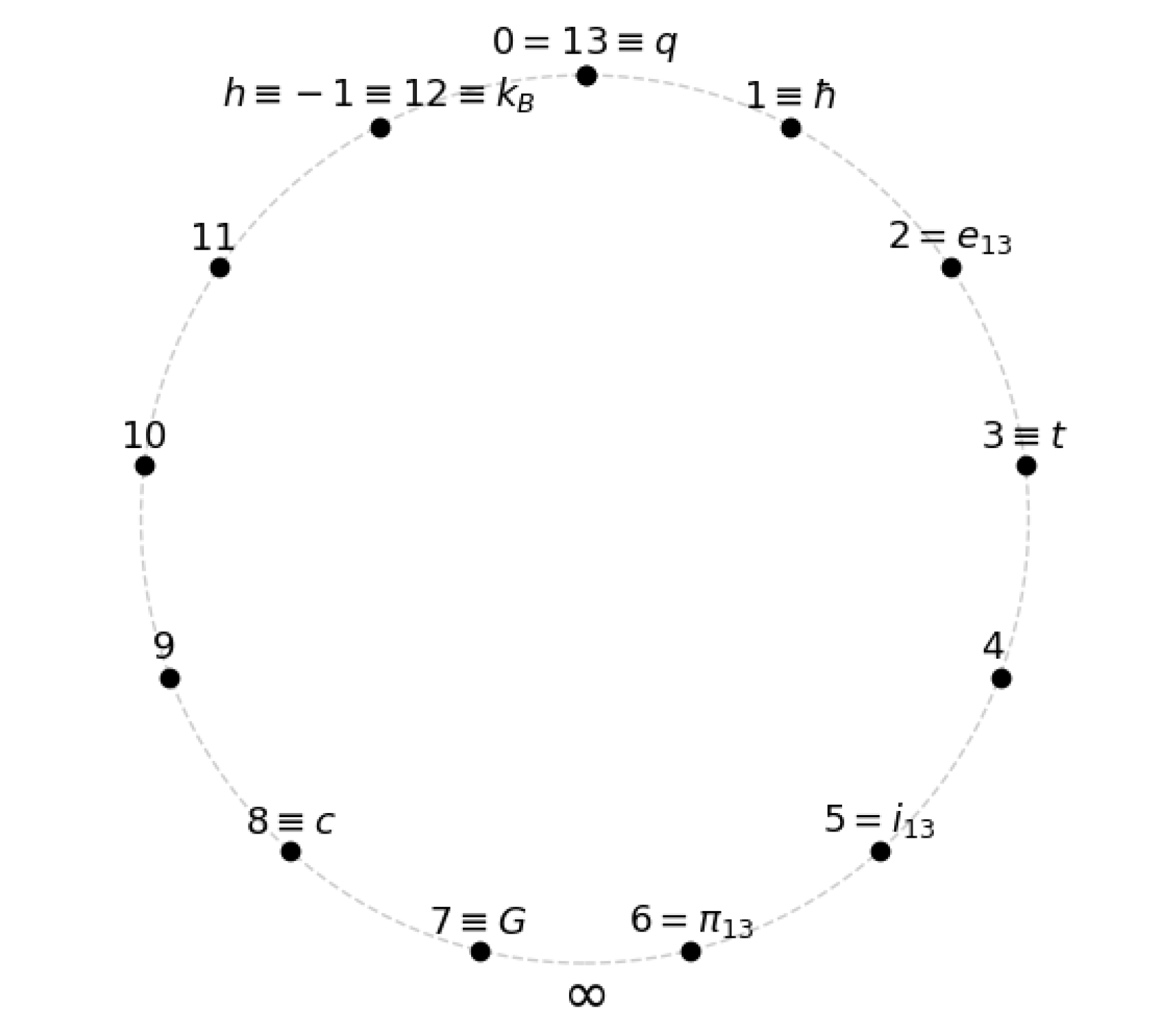
Table 2.
Canonical constants in the finite relational algebra.
| Continuum symbol | Finite value in | Characterizing property |
|---|---|---|
| ℏ | 1 | Additive generator of the ring, quantization increment |
| h | Full quantum of action, | |
| c | Future-oriented multiplicative quarter-turn, | |
| G | Inverse minimal-action primitive root | |
| Signed involution, entropy-energy conversion factor |
Disclaimer/Publisher’s Note: The statements, opinions and data contained in all publications are solely those of the individual author(s) and contributor(s) and not of MDPI and/or the editor(s). MDPI and/or the editor(s) disclaim responsibility for any injury to people or property resulting from any ideas, methods, instructions or products referred to in the content. |
© 2025 by the authors. Licensee MDPI, Basel, Switzerland. This article is an open access article distributed under the terms and conditions of the Creative Commons Attribution (CC BY) license (http://creativecommons.org/licenses/by/4.0/).
Copyright: This open access article is published under a Creative Commons CC BY 4.0 license, which permit the free download, distribution, and reuse, provided that the author and preprint are cited in any reuse.


