
Submitted:
17 June 2025
Posted:
18 June 2025
You are already at the latest version
Abstract
The nonlinear differential-algebraic equations (DAE) governing the six-degree-of-freedom motion of a fixed-wing aircraft consists of several coupled elements describing the linear (translational) motion, angular motion, and intermediate flight variables. In this work, we start with a generic mathematical framework for the equations of motion (EOM) in flight mechanics (flight dynamics) with six degrees of freedom (6-DOF) for a general (non-symmetric) airplane, and this mathematical framework incorporates body axes (fixed in the airplane at its center of gravity), inertial axes (fixed in the earth/ground at the take-off point), wind axes (aligned with the flight path/course), spherical flight path angles (azimuth angle measured clockwise from the geographic north, and elevation angle measured above the horizon plane), and spherical flight angles. We then customize these equations of motion to derive a customized version suitable for inverse simulation, where a target flight trajectory is specified while a set of corresponding necessary flight controls to achieve that maneuver are predicted. We then present a numerical procedure for integrating the developed inverse simulation system in time, utilizing symbolic mathematics, the explicit fourth-order Runge-Kutta numerical integration technique, and expressions of the finite difference method, such that the four necessary control variables (engine thrust force, ailerons’ deflection angle, elevators’ deflection angle, and rudder’s deflection angle) are estimated as discrete values over the entire maneuver time, and these values enable the airplane to achieve the desired flight trajectory as specified by three airplane’s inertial Cartesian coordinates along with the Eulerian roll/bank angle. The proposed numerical procedure of flight mechanics (flight dynamics) inverse simulation is demonstrated through an example representative of the Mirage III French fighter airplanes.
Keywords:
aircraft
; flight
; dynamics
; ailerons
; elevators
; rudder
1. Introduction
Mathematical modeling and numerical simulations are important tools for describing various nonlinear complex phenomena and processes, as well as implementing computer-aided design (CAD), computational fluid dynamics (CFD), and automatic control [1,2,3,4,5,6,7,8,9,10,11,12,13,14,15,16]. Flight mechanics (also called flight dynamics) is one of the engineering fields that benefits largely from mathematical modeling and numerical simulation; because simple analytical reduced-order solutions in aerospace applications and dynamics are typically not available except under very restrained conditions, and experimental techniques through wind-tunnel tests (WTT) and flight tests are stochastic (non-deterministic), expensive, limited in terms of the amount of data that can be measured directly, and sometimes intrusive (influencing the domain being tested) [17,18,19,20,21,22,23,24,25,26].
Inverse simulation (InvSim) in flight mechanics (flight dynamics) is a normative category of flight mechanics modeling in which a desired flight trajectory (flight maneuver or flight mission) is specified through a number of inputs, while the corresponding flight controls (the model-based feedforward control variables) needed to achieve this trajectory are predicted; the opposite of this modeling process is called forward flight mechanics simulation, which is an exploratory category of flight mechanics modeling [27,28,29,30,31,32,33]. Accurate inverse simulation flight mechanics (flight dynamics) modeling facilitates advanced modes of transportation through pilotless (autonomous) aviation activities, such as regular electrified urban air mobility (e-UAM) trips within smart cities or between neighbor cities, powered by clean renewables; although additional real-time control systems for external perturbation suppression should be augmented [34,35,36,37,38].
This work is a sequel to a previous part in which we provided a detailed mathematical framework for general modeling the motion for a fixed-wing aircraft, and this framework has several advantages; namely: (1) all six degrees of freedom (6-DOF) are included, (2) the singularity of upward/downward vertical flight (encountered in a traditional Euler-angle representation) is avoided, (3) linear (translational) momentum equations are transformed such that the order of terms does not suffer from large discrepancy under fast dynamics, (4) the assumption of airplane symmetry is eliminated, (5) the aerodynamic details for all the flight-dependent aerodynamic/stability coefficients are clearly expressed, (6) three sets of axes: inertial ground/earth axes, body-fixed axes, and wind axes are utilized instead of using the Euler angles directly to describe the attitude of the airplane, (7) two flight-path angles (azimuth and elevation) are utilized as an intermediate spherical coordinate system; allowing the separation of the flight path direction relative to air (the airplane course) from the airplane attitude relative to the ground (the airplane heading), (8) only scalar equations (rather than vector equations or quaternions) are utilized, which simplifies the implementation process as a digital flight mechanics simulator, (9) the variation of the air density with altitude is accounted for using the international standard atmosphere (ISA) model for air as an ideal homogeneous gas, and (10) the model can be easily adjusted to specific airplane conditions through user-defined input parameters, and also specialized airplane features (such as a nonlinear lift coefficient profile) can be handled through minor modifications [39,40,41,42,43,44,45,46,47,48,49,50,51,52,53,54,55,56,57,58,59,60,61,62,63,64,65].
The current work can be used within a curriculum module in college programs related to aeronautics, numerical methods, or control [66,67,68,69,70,71,72,73,74]
We do not address here social or economic aspects of flight and aviation modeling [75,76].
In the current work, the previously explained general nonlinear differential-algebraic equations (DAE) for flight mechanics are reformulated such that they fit specifically inverse simulation flight dynamics, and an algorithm is presented to numerically integrate these equations of motion (EOM) in a simple explicit process that does not require solving an algebraic system of equations, with the use of the fourth-order Runge-Kutta (RK4) numerical integration method; also numerical differentiation expressions based on the finite difference method (FDM) may be used [77,78,79,80,81,82,83,84]. We implement this proposed numerical procedure as a computer code, and demonstrate its utilization while inversely simulating a continuous-double-roll maneuver with a set of airplane data that nearly corresponds to the Mirage III fighter aircraft, produced by the French aerospace company Dassault Aviation [85,86,87].
2. Research Method
2.1. Problem Statement
The inverse simulation (InvSim) flight mechanics algorithm proposed here considers the airplane as a MIMO (multi-input multi-output) control system, with four inputs and four outputs. The four inputs are specified as the inertial (ground-referenced) Cartesian coordinates () of the airplane’s center of gravity (CG), and these coordinates may be described as analytical functions of time or as discrete values recorded with the corresponding time values (or with a uniform time step, . The () coordinate represents the signed distance traveled by the airplane in the positive geographic north direction from the initial flight point (the take-off point). The () coordinate represents the signed distance traveled by the airplane in the positive geographic east direction from the initial flight point. The () coordinate represents the signed distance traveled by the airplane toward the earth’s center from the initial flight point, and thus this coordinate is expected to have negative values except during parts of the maneuver where the airplane descends to an altitude below the initial altitude. Figure 1 illustrates these three input coordinates. The term “gravity axis” here refers to the inertial axis pointing toward the earth’s center (perpendicular to the horizon plane), and it is opposite to the “altitude axis” that is also perpendicular to the horizon plane but points toward the sky. The origin of these ground-referenced rectangular coordinates is the initial flight point (the first location of the trajectory to be inversely simulated).
In the current work, the altitude of the airplane’s center of gravity as measured from the mean sea level (MSL) is designated by the symbol (), and the initial altitude is designated by the symbol (). Therefore, the gained height of the airplane’s center of gravity above the initial trajectory point is (); which should be equal to the negative value of the () coordinate. Therefore,
The fourth input to the airplane model is the bank angle (also called roll angle) in radians, which is one of the three Euler angles, and it describes the lateral attitude of the airplane. If the starboard (right) and port (left) tips of the wing are at the same vertical position (having the same altitude), then the bank angle () is zero. By convention, the bank angle is positive if the wing’s starboard tip tilts down (and the wing’s port tip tilts up) [88,89]. Figure 2 illustrates the bank angle when it has a positive value.
The four outputs from the inverse simulation flight mechanics model here are the four flight controls (four control variables), computed as four discrete series of values (four numerical vectors). These controls are in charge of adjusting the speed and orientation of the airplane, such that the input conditions are satisfied. These controls are:
- The engine thrust force (), in newtons. This control can also be an electric propulsion force in the case of using an electric propeller or an electric ducted fan (EDF) [90,91,92,93,94]. This electrification has an environmental advantage through eliminating combustion emissions [95,96,97,98,99,100,101,102,103,104,105,106,107,108]. Hydrogen-based propulsion is also preferred environmentally due to the lack of harmful greenhouse gas (GHG) emissions [109,110,111,112,113,114,115,116,117,118]. The thrust force is a non-negative quantity.
- The ailerons’ deflection angle (), in radians. This deflection is primarily in charge of the rolling degree of freedom. This deflection angle is positive when the hinged starboard aileron tilts up and simultaneously the hinged port aileron tilts down (which induces a positive bank angle, ).
- The elevators’ deflection angle (), in radians. This deflection is primarily in charge of the pitching degree of freedom. This deflection angle is positive when both hinged elevators tilt down (which induces a positive pitch angle, , where the airplane’s nose tilts up).
-
The rudder’s deflection angle (), in radians. This deflection is primarily in charge of the yawing degree of freedom. This deflection angle is positive when the hinged rudder tilts toward the port/left side (which induces a positive yaw angle “heading angle”, , where the airplane’s nose tilts toward the port side).Figure 3 illustrates these four flight controls.
2.2. Research Approach
In order to solve the stated problem in the previous subsection, symbolic mathematical manipulation is combined with computational methods to build and present here a proposed numerical algorithm for solving the inverse simulation flight mechanics problem. A general set of flight mechanics equations of motions are first presented. These equations are then reformulated to be in the inverse simulation InvSim) form, such that the four output flight controls can be obtained for specified inputs (trajectory coordinates and bank angle). Then, a proposed algorithm is presented, which allows numerically integrating the reformulated coupled differential-algebraic equations (DAE) in a simple way that can be implemented using a general-purpose computer programming language, without the need for specialized capabilities [119,120]. We here use the MATLAB/Octave programing language, which is a high-level interpreted language especially suitable for numerical computations, although other programing languages (such as Python) can also be used [121,122,123,124,125,126].
The success of the proposed computational InvSim algorithm and the underlying mathematical model is supported by numerically simulating an example flight maneuver. We obtained some symbolic expressions for needed derivative terms manually using normal calculus rules; and independently using Mathematica (a popular software tool for symbolic mathematics and computations that has been used in many research works before), and both sets of obtained expressions were exactly compatible [127,128,129,130,131,132,133,134,135,136,137].
3. General Equations of Motion
In this part, we present part of a flight mechanics mathematical framework, which is not optimized specifically for inverse simulations. The equations of motion listed in this section are not just the six main equations (three linear/translational momentum equations and three angular/rotational momentum equations) for a six-degree-of-freedom flight. Instead, auxiliary intermediate equations are also listed, since they need to be considered along with the six main equations as a whole integrated coupled system.
3.1. Angular Velocity Vector in Body Axes
The roll rate (), pitch rate (), and yaw rate () are related to the Euler angular rates or Euler rates () that are the time derivatives of the Euler angles, according to
Figure 4 illustrates the three Euler angles () which describe the three-stage rotational transformation from the inertial axes system (north, east, gravity) into the body-fixed axes system ().
3.2. Linear-Momentum Equations and Equilibrium
The linear-momentum equations are transformed from the orthogonal Cartesian system into the body-fixed spherical wind axes, whose coordinates are the velocity magnitude (), the sideslip angle (), and the angle of attack (). These three variables () can be viewed as spherical coordinates, with the velocity magnitude () being the radial coordinate. The forward wind axis is tangent to the flight path and thus coincides with the total velocity vector (velocity of the airplane’s center of gravity). The sideslip angle () represents a rotational transformation of the wind axes such that the rotated lies in the airplane’s fixed plane (the airplane’s midplane), which is the plane of symmetry for symmetric airplanes.
The condition ( = 0°) means that the incoming airflow relative to the airplane is symmetric with respect to the midplane. The angle of attack () represents a subsequent rotational transformation (after the rotational transformation) such that the twice-rotated wind axes () coincide with the body-fixed axes (). Figure 5 illustrates the wind angles ( and ), as well as the relation between the wind axes system () and the body axes system ().
Although our definition for the angle of attack (AoA, ) discussed above, as a second angle of axes transformation, implies that in the absence of any sideslip ( = 0) and when = 0°, the longitudinal body axis () coincides with the forward wind axis (). This configuration corresponds to a horizontal steady-level flight with zero tilts by the airplane (the body-fixed plane is parallel to the horizon plane), and we refer to this configuration here as the “equilibrium” condition of flight. However, despite the horizontal orientation of the airplane’s body, and the zero value assigned to the angle of attack () as per our definition here, aerodynamic principles demand that there must be an exerted lifting force to counteract the weight of the airplane during an equilibrium flight.
The equilibrium lift force may require either using a nonsymmetrical (cambered) wing airfoil section while keeping the wing mounted parallel to the main airplane body (the fuselage), such that a non-zero upward lifting force can be induced even when the airplane is flying horizontally through the ambient air with its nose-to-tail longitudinal axis also being horizontal; or mounting the wing (which can be cambered or symmetric) at a small tilt angle called the angle of incidence or mounting angle (), such that when the airplane flies horizontally with a horizontal longitudinal body axis, there is still a non-zero lifting force that achieves the equilibrium condition because the tilted wing now faces the air asymmetrically, causing the air pressure at the lower surface of the wing to be higher than the air pressure at the upper surface of the wing due to the asymmetric air flow around the wing, and this leads to the upward lifting force component (combined with an aerodynamic drag force component) [138,139,140,141,142,143,144,145,146,147,148,149,150,151,152]. In the current study, we adopt the latter choice; thus, we assume that the wing is installed into the fuselage at an angle of incidence () that satisfies the equilibrium condition; and this tilt angle () is excluded from the angle of attack () used in the modeling and numerical simulation discussed here.
In the presented flight mechanics model here, the angle of attack () excludes any equilibrium angle between the velocity vector of the airplane’s center of gravity (whose magnitude is ) and the wing’s mean chord line (the virtual straight line connecting the leading edge with the trailing edge of the wing of an airfoil section) [153,154,155,156,157,158]. Therefore, the symbol () that appears in this study means the change in the conventional angle of attack (denoted here by the symbol ; and it includes the angle of incidence or the tilt of the wing relative to the velocity vector of the airplane) from its equilibrium conventional value (), which is assumed to be equal to the angle of incidence in the current work. Therefore, we have
In aeronautics, the equilibrium conventional angle of attack () is not truly a constant, but it depends on the flight speed and air density (this, on the flight altitude). Thus, our assumption of equality between the equilibrium conventional angle of attack and the angle of incidence () implies that the angle of incidence is effectively adjustable also, for example through using movable flaps attached to the wing and these allow mildly adjusting the wing’s effective angle of incidence [159,160,161].
Figure 6 illustrates the difference between the angle of incidence () and the angle of attack (), and also shows how they differ from the Euler pitch angle () discussed in the previous subsection, and from the elevation flight path angle () that describes the climb angle of the airplane based on its course of flight as a point particle.
The linear-momentum equations (with its components corresponding to the wind axes) are
where Equation (8) is the component of the vector linear momentum equation, Equation (9) is its component, and Equation (10) is its component.
In the above equations, () is the airplane mass, () is the wing planform area, () is the thrust force, () is the Euler’s pitch angle, () is the gravitational acceleration, () are nondimensional force coefficients (to be discussed later), and () is the dynamic pressure defined as [162,163,164,165,166]
where () is the air density.
The gravitational acceleration is treated here as a universal constant with the value of 9.81 m/s2
It may be useful to add here that if the linear/translational equations of motion are formulated along the body-fixed axes; then their three components along the longitudinal axis (), the lateral body-fixed axis (), and the third/bottom body-fixed axis (); respectively; are
These are the three components of the following vector linear-momentum equation in the body-fixed axes:
where () are the three components of the velocity along the three body-fixed axes (). The right-hand side in the above vector equation is the total applied forces on the airplane. The first part represents the aerodynamic forces, the second part represents the weight, and the third part represents the thrust force.
3.3. Angular-Momentum Equations
A derived geometric constant () needs to be computed once, and this constant is the determinant of the symmetric inertia tensor. The three diagonal components of this tensor are the moments of inertia (or rectangular moments of inertia) for rotations perpendicular to the three corresponding body axes (centered at the airplane’s center of gravity), which are positive numbers for a rigid body; while the off-diagonal elements are the products of inertia, which can be negative, zero, or positive numbers [167,168,169,170,171,172,173].
The constant () us expressed mathematically as
The SI unit of each component of the inertia tensor is kg.m2, and thus the SI unit of () is kg3.m6. The six components of the inertia tensor are further explained in Table 1.
For a symmetric airplane, the left (port) half is identical (but reflected) to the right (starboard) half; and in such a left-right symmetric condition, only the product of inertia in the symmetry midplane plane () is non-zero ( ≠ 0) in that case [174,175,176].
Because the rotational equations of motion are expressed in the body-fixed axes and the above inertia terms are formulated also with respect to the body-fixed axes, these inertia terms are considered invariant constants in the rotational equations of motion.
Three auxiliary moments () are defined through three algebraic equations as
Finally, the main rotational equations of motion for the airplane about its body axes are
In the special case of a symmetric airplane, the seven equations presented in the current subsection, namely Equations (13-19), can be replaced by only three differential angular-momentum equations that are listed below; which can be derived from Equations (13-19) after setting ( = 0) and ( = 0) and performing some mathematical manipulation [177,178,179,180,181,182,183,184,185].
which can be further manipulated and expressed using the alternative symbols for the inertia terms as
3.4. Inertial Velocity
The equations relating the rates of the ground-referenced inertial coordinates () to the velocity magnitude and the spherical flight path angles (azimuth flight path angle , and elevation flight path angle ) are
Figure 7 illustrates the two spherical flight path angles ( and ), which describe the flying course (direction) of the airplane, as a particle, with respect to the inertial origin (the initial trajectory point) using the three spherical coordinates () as an alternative to the Cartesian inertial velocity components ().
3.5. Flight Path Angles
Two additional algebraic equations relate the two flight path angles () to the three Euler angles () and the two wind axes angles (, ) are provided below [186,187,188,189,190,191].
From the two above equations; it can be proven that in the condition of equilibrium flight ( = 0, = 0), the Euler yaw angle () “also called heading angle” becomes equal to the azimuth flight path angle (), and the Euler pitch angle () becomes equal to the elevation flight path angle ().
3.6. Three Aerodynamic Forces
The three body-axes aerodynamic forces acting on the airplane are expressed as
In the above equations, () is the aerodynamic force along the longitudinal body-fixed axis, and its unit vector exactly coincides with the unit vector of the thrust vector; () is the aerodynamic force along the starboard lateral body-fixed axis; and () is the aerodynamic force along the third (bottom) body-fixed axis.
3.7. Three Moments
The total moment vector is resolved into three components (which we also refer to as three moments) along the body axes. These moments are expressed in terms of nondimensional moment coefficients () as
In the above equations, () is the rolling moment about the longitudinal body-fixed axis (), () is the pitching moment about the lateral body-fixed axis (), and () is the yawing moment about the third/bottom body-fixed axis (). In addition, () is a characteristic length for the pitching moment (longitudinal stability), such as the mean wing chord [192,193,194]. On the other hand, the characteristic length () pertains to the rolling moment (lateral stability) and yawing moment (directional stability), and it can be the wing span [195,196,197,198,199].
3.8. Aerodynamic and Stability Coefficients
The aerodynamic lift coefficient (), aerodynamic drag coefficient () [200,201,202,203], and aerodynamic side-force coefficient () are wind-axes nondimensional quantities from which the body-axes aerodynamic coefficients () can be obtained [204,205,206,207,208,209,210,211].
The lift coefficient is modeled here as being directly related to the conventional angle of attack () as
where () is the lift coefficient at zero conventional angle of attack, and () is the gain in the lift coefficient per unit increase in the angle of attack (when expressed in radians), and both values are treated as constant parameters.
As mentioned earlier in subsection 3.2, the term “angle of attack” () used in the proposed flight mechanics simulation modeling here is the change (either positive or negative) in the conventional angle of attack from its equilibrium value (), which is assumed to be equal to the angle of incidence for the wing (). Therefore, the lift coefficient () is related to the modeling/simulation angle of attack () as
Regardless of the lift coefficient being expressed as a function of the conventional angle of attack () as in Equation (37), or being expressed as a function of the modeling/simulation angle of attack () as in Equation (38), it has the same constant slope (). At any given value of (), the angular difference () is equal to the equilibrium value of the conventional angle of attack (; and it is computed from the force balance between the weight of the airplane () and the equilibrium lift force (), where () is the lift coefficient at equilibrium flight. Therefore,
Combining the above defining equation for the equilibrium lift coefficient with Equation (37) that relates the lift coefficient () linearly with the conventional angle of attack () gives
and this leads to an explicit expression for the conventional equilibrium angle of attack ( as
This conventional equilibrium angle of attack ( is approximately constant if the dynamic pressure is nearly constant (), and this implies that the air density and the flight speed are nearly unchanged, and this is a valid assumption in steady-level flight.
Figure 8 illustrates the linear dependence of the lift coefficient () on the modeling/simulation angle of attack (), which is the default angle of attack in the current work, and on the conventional angle of attack () as described above. This linear dependence is appropriate as long as the airplane is away from aerodynamic stall conditions [216,217,218,219,220,221,222].
Through the drag polar relationship, the drag coefficient depends on the lift coefficient as [223,224,225]
where () and () are additional aerodynamic constants.
The side-force coefficient depends on the sideslip angle as
After knowing the wind-axes aerodynamic coefficients (), the body-axes aerodynamic coefficients () can be obtained using trigonometric projections as
The body-axes total-moment coefficients () are modeled as
where () are nondimensional constant parameters, while () are dimensional constant parameters having the unit of 1/rad, () is the ailerons’ deflection angle in radians, () is the elevators’ deflection angle in radians, and () is the rudder’s deflection angle in radians.
3.9. Air Density and Speed of Sound
The variation of the air density with the altitude () is governed here by the International Standard Atmosphere (ISA) model. Up to an altitude of about 11,000 m above mean sea level, the stratosphere layer of the air exists, in which the air temperature decreases linearly with altitude, while the density declines nonlinearly with altitude at a faster rate according to [226,227,228,229,230,231,232,233,234].
where () is the lapse rate magnitude, taken as 0.0065 K/m; and () is the ideal gas constant for air, which is the universal molar gas constant divided by the molecular weight, and this gas constant for air is 287 J/kg.K [235,236,237,238]. In the previous equation, the constant 1.225 is the standard sea level air density in kg/m3 (); and the constant 288.15 is the standard sea level absolute temperature in kelvins (), which corresponds to 15 °C [239,240,241,242,243].
Although the ISA model is based on geopotential altitudes for estimating the air density, we here utilize the true geometric (orthometric) altitude [244,245,246,247,248,249,250,251,252,253,254,255,256]. This simplification is aligned with our treatment of the gravitational acceleration as a universal constant. We assessed the difference in the two types of altitudes, and we found that the difference in the stratosphere layer of interest here is small as shown in Table 2.
The percentage deviations in the above table are very small, much less than 1%. These percentage deviations were computed as [257]
The relationship between the geometric altitude () and geopotential altitude (denoted by ) is
where () is the mean radius of the earth, and it is taken here as 6,371,000 m [258,259,260,261,262].
In Table 3, we further assess the influence of using a geometric altitude rather than a geopotential altitude when using Equation (37) for computing the air density. At a geometric altitude of 5,000 m for example; the air density should be computed strictly speaking at the slightly-lower geopotential altitude of approximately 4,996 m. Similarly, the air density computed at a geopotential altitude of 5,000 m strictly speaking corresponds to the slightly-higher geometric altitude of approximately 5,004 m. However, the values in the table show that these three densities are nearly the same, and the error incurred by the simplifying assumption of using the geometric altitude in lieu of the geopotential altitude leads to a marginal error in the air density that is below 0.05% at altitudes near 5,000 m; corresponding approximately to the middle of the stratosphere layer of the atmosphere.
Similarly, Table 4 assesses the expected error in the air density but at higher altitudes near 10,000 m; located close to the upper end of the stratosphere layer of the atmosphere. Although the error grew (nonlinearly) as the altitude increased, it remains very small, below 0.2%.
Many commercial transport airplanes fly at cruising altitudes below 11 km, thus the stratospheric formula is adequate for them [263,264,265,266,267,268,269,270,271]. For higher altitudes, as in military aircraft, another expression for the air density should be used, which corresponds to the tropopause layer of the atmosphere; it is an interspheric layer between the lower troposphere layer and the upper stratosphere layer, extending approximately between the altitudes 11,000 m and 20,000 m [272,273,274,275,276,277]. In the tropopause layer of the atmosphere, the temperature is treated as constant (with a value of –56.50 °C or 216.65 K, making it an isothermal layer. Therefore, the decline of the air density with the altitude within the tropopause layer follows a different profile than the one described earlier for the non-isothermal troposphere layer. This decline is described as
where the value (11,000) is the altitude (in meters) at the bottom edge of the tropopause layer, the value (0.3636309) is the air density at 11,000 m () in kg/m3, as computed by the tropospheric density equation, and this value is also the air density at the bottom edge of the tropopause layer; and the value (216.65) is the absolute temperature (in kelvins) of air within the tropopause layer ().
It is worth mentioning that the decline of the air density in the non-isothermal troposphere layer is slower than its decline in the isothermal tropopause layer, because the drop of temperature in the non-isothermal troposphere layer has a compressive effect on air, causing its density to tend to increase, however the drop in the pressure due the diminishing weight of the above air column causes a stronger expansive effect of decreasing the density, which ultimately declines with the altitude [278,279,280,281,282]. In the isothermal tropopause layer, the compressive temperature effect is eliminated, thereby magnifying the expansive pressure effect, and thus the air density declines faster with the altitude. To demonstrate this faster rate of density decline in the isothermal tropopause layer, applying Equation (54) for the tropospheric density to an altitude of zero (= 0) gives an extrapolated benchmarking value sea-level air density of 2.0624 kg/m3, which clearly exceeds the true sea level value of 1.225 kg/m3 [283,284].
Although the speed of sound () in air is not an essential variable in the presented flight mechanics model, it is still an important property in aeronautics in general, because the ratio between the airplane speed () and the speed of sound is the nondimensional Mach number () that serves as a criterion for determining the regime of flight as well as the possible occurrence of special phenomena such as shock waves. The Mach number is defined as
The flight regime with is subsonic, the flight regime with is transonic or sonic, the flight regime with is supersonic, while the condition corresponds to the hypersonic flight regime [285,286,287,288,289,290,291,292].
The speed of sound for air, as an ideal gas, depends on its absolute temperature () and the specific heat ratio (the ratio of specific heat capacities, or the adiabatic index, ) as [293,294,295]
In the troposphere layer of the atmosphere (the non-isothermal layer adjacent to the ground), the air absolute temperature is estimated according to the lapse rate ( K/m) as
In the tropopause layer of the atmosphere (the isothermal layer next to the troposphere layer), the air absolute temperature is treated as a constant value of 216.65 K. Thus,
The specific heat ratio is treated here as a constant with a value of 1.4, which is commonly assigned to ambient air [296,297,298,299].
γ=1.4
4. Summary of Equations, Variables, and Constants
In the current section, we provide a summary of the overall six-degree-of-freedom (6-DOF) fluid mechanics problem in terms of the mathematical structure.
4.1. Summary of Equations
The current fluid mechanics problem is described by a nonlinear differential-algebraic equations (DAE) system, consisting of 35 equations that are either ordinary differential equations (ODE) or algebraic equations. These 35 scalar equations can be grouped into nine categories as shown in Table 5. It should be noted that these groups are not mathematically decoupled; the grouping is based on the scope of use for the equations.
4.2. Summary of Variables
The aforementioned 35 flight mechanics equations have 39 independent variables, which are listed in Table 6 as categorized groups. It should be noted that constant parameters that appear in the differential-algebraic equations (such as the wing planform area and the airplane mass) are not included among the flight variables, because they are invariant during the entire flight trajectory. In addition, the time derivative of a flight variable is not considered an additional variable.
The difference between the number of equations and the number of variables is four, and this is the number of input constraints that should be specified in order to be able to integrate the flight mechanics system and obtain a unique solution. The four constraints in the case of our inverse simulation (InvSim) flight mechanics model are the profiles of the three inertial coordinates () and the profiles of the bank angle (). The output variables to be obtained by the InvSim flight mechanics solver are the discrete profiles of four airplane controls, which are the thrust and the three deflection angles of the control surfaces (). The remaining 31 variables (such as the angle of attack , and the Euler pitch angle ) are intermediate quantities that can evolve over time during the flight maneuver in response to changes in other related variables.
4.3. Summary of Constants
In addition to the 39 flight variables (that generally vary during the flight maneuver), various constant parameters need to be defined, and these values remain unchanged during the entire flight simulation. The total number of constants in the proposed InvSim model is 30, which are classified as 29 parameters for describing the airplane and its performance, and one parameter related to the trajectory (the initial altitude). These 30 constant parameters are summarized in Table 7, which are organized as related groups.
It should be noted that physical universal constants are not counted among the 30 parameters, because these are not customizable quantities. These universal constants are
- Gravitational acceleration ( = 9.81 m/s2)
- Tropospheric lapse rate ( = 0.0065 K/m)
- Ideal gas constant for air ( = 287 J/kg.K)
- Standard sea-level air density ( = 1.225 kg/m3)
- Standard sea-level air absolute temperature ( = 288.15 K)
- Standard altitude of the troposphere-tropopause transition (11,000 m)
- Standard air density at the troposphere-tropopause transition ( = 0.3636309 kg/m3)
- Standard air absolute temperature within the tropopause layer ( = 216.65 K)
While it is possible to upgrade the model by treating the gravitational acceleration as a function of altitude (in this case, the number of flight variables increases from 39 to 40); the gain from this upgrade is not justified. This change largely increases the mathematical complexity of the model, where the time derivative of the gravitational acceleration appears in the mathematical expressions, while such a derivative is practically zero.
To demonstrate this (and justify treating the gravitational acceleration as a universal constant), we first point out that the altitude-dependent gravitational acceleration () declines with the geometric altitude according to the following quadratic relationship:
At a geometric altitude of 11,000 m (which is the upper limit of the troposphere layer), the altitude-dependent gravitational acceleration is 99.656 % of its approximated constant value (at sea level); and a higher geometric altitude of 20,000 m (which is the upper limit of the tropopause layer), the altitude-dependent gravitational acceleration drops further to 99.375% its approximated constant value. Thus, the relative drops in the gravitational acceleration at 11,000 m and 20,000 m geometric altitudes are only 0.344% and 0.625%; respectively. As dimensional drops in the altitude-dependent gravitational acceleration from a sea-level value of 9.81 m/s2; the respective drops at 11,000 m and 20,000 m geometric altitudes are 0.0033788 m/s2 and 0.006130 m/s2; respectively. At a rate-of-climb (RoC) of 2,000 ft/min (33.33 ft/s, 10.16 m/s, or 36.58 km/h), which is typical for a commercial jet airplane, an altitude of 11,000 m (36,089 ft) can be reached after a continuous climb for about 1,083 seconds (about 18 minutes); and this means that the average rate of change of the altitude-dependent gravitational acceleration in this case is approximately 3.12×10⁻⁶ m/s3, which is nearly zero [300,301,302,303,304,305,306,307]. Although high-performance fighter airplanes may achieve much higher climb rates and descent rates, such as 20,000 ft/min (10 times the typical rates for commercial jet airplanes), the time rate of change in the altitude-dependent gravitational acceleration in such cases remains negligible [308,309,310,311,312,313,314].
For estimating the speed of sound in air, one more universal constant was utilized, which is the nondimensional specific heat ratio [315] (or adiabatic index) for air, which is set at the reasonable value of 1.4.
- Specific heat ratio for air ( = 1.4)
Although the specific heat ratio for air, as an ideal gas, is actually a function of its temperature, which is a function of the altitude within the troposphere layer; treating the specific heat ratio as a universal constant as adopted here is appropriate given the narrow range of temperatures for atmospheric air during an airplane flight [316]. In this case of a constant specific heat ratio, air is assumed to be a “calorically perfect” gas, which is a special simplified case of ideal gases [317,318]. For air, the specific heat ratio is 1.4022 at 288.15 K (15.00 °C) and it increases to 1.4027 at 216.65 K (–56.50 °C); while it drops to 1.4015 at 323.15 K (50.00 °C); and these values show the weak deviation from the nominal used value of 1.4 [319].
5. InvSim Customized Equations of Motion
In this part, we present a variant of the general fluid mechanics equations of motion, which is adapted for use in an inverse simulation (InvSim) mode. These customized equations are presented as nine groups in the next subsections, with a different order than the one presented earlier for the general equations in section 3; this change in order facilitates explaining the rationale behind the need for additional derivative expressions beyond those appearing in the general flight mechanics equations.
In summary, the three unknown control deflection angles are computed from three algebraic equations, while the unknown thrust force is computed among eight flight variables through a classical fourth-order Runge-Kutta method (RK4) for integrating a system of nonlinear ordinary differential equation (ODE) [320,321,322,323,324,325].
5.1. InvSim Aerodynamic and Stability Coefficients
The formulas presented earlier in subsection 3.8 for the aerodynamic lift coefficient (), aerodynamic drag coefficient (), the side-force coefficient (), and the three body-axes aerodynamic coefficients () remain in use in the transformed InvSim mode of the flight mechanics equations of motion. For completeness, these expressions are repeated here.
However, the original expressions for the body-axes total-moment coefficients () are restructured into three explicit expressions to obtain the three control surface deflection angles. The original expressions for the body-axes total-moment coefficients () are repeated below to facilitate the derivation of the restructured ones.
From Equation (48), the restructured explicit expression for the necessary control surface deflection angle for the elevators () can be obtained as
Solving Equations (47 and 49) simultaneously for the necessary control surface deflection angle for the ailerons () and the rudder () gives
The coupling between the rolling and yawing moments is noticeable from Equations (47 and 49), and these two moments are together decoupled from the pitching moment as indicated by Equation (48); this behavior is known for fixed-wing airplanes [326,327,328,329,330,331].
5.2. InvSim Three Moments
In subsection 3.7 of the original general flight mechanics formulation, the total moment vector was resolved into three components (three moments; ) along the body axes (); and these body-referenced moments were expressed in terms of three nondimensional moment coefficients (), respectively. However, in the previous subsection 5.1, we showed that the proposed InvSim flight mechanics formulation requires the values of these nondimensional moment coefficients to algebraically obtain the corresponding control surface deflection angles ().
Therefore, the original expressions for () are inverted here to be explicit expressions for (), as follows:
5.3. InvSim Angular-Momentum Equations
In the part of the original general flight mechanics formulation covered earlier in subsection 3.7, algebraic expressions for three auxiliary moments () were given as functions of the body-referenced angular velocity components () and body-referenced total moments (); with the body-axes inertia components () being constant geometric parameters. These expressions are repeated below.
Also, the original general flight mechanics formulation in subsection 3.7 included three main rotational equations of motion for the airplane about its body axes, which are repeated below.
As explained before, () is the determinant of the inertia tensor.
However, according to the discussion given in the previous subsection, the body-referenced total moments () are needed in order to obtain the corresponding nondimensional moment coefficients (). These body-referenced total moments are obtained by solving simultaneously the above system of three equations, Equations (17-19), for the auxiliary moments () as three explicit expressions whose right-hand side include the body-referenced angular accelerations (). The resultant explicit symbolic expressions for () and () are complicated and thus are not shown here; but we designate them by the placeholder symbols () and (), respectively. However, the explicit symbolic expressions for () is simple enough to be shown here, and it is given below and we designate it by the symbol () to distinguish it from the original explicit expression in Equation (16) that also has () in its left-hand side as a single quantity, but that original expression is not directly used in the proposed InvSim algorithm presented here.
After the values of the auxiliary moments become known at a given time station, the body-referenced total moments () can be computed using an adapted version of the equations that defined the auxiliary moments (); namely Equations (14, 15, 16), respectively. These adapted equations are suitable for computing the numerical values of (), and they have the following form:
5.4. InvSim Angular Velocity Vector in Body Axes
The expressions relating the body-referenced roll rate (), body-referenced pitch rate (), and body-referenced yaw rate () to the Euler rates and Euler angles remain the same. These expressions were presented in Equations (2-4), and are repeated below.
The above algebraic expressions for the body-referenced angular velocities () are used to find initial values () for them at the beginning of the maneuver’s numerical simulation, at = 0.
According to the InvSim customized expressions () discussed earlier in the previous subsection 5.3 for the auxiliary moments (), it is required to know the values of the derivatives of the body-referenced angular velocities () in order to be able to compute the dependent values of the auxiliary moments (). Expressions for these three body-referenced angular accelerations () are obtained symbolically by direct differentiation of the expressions for () as presented in Equations (2-4). The resultant expressions for the body-referenced angular accelerations are
5.5. InvSim Flight Path Angles
The obtained explicit expressions for the three body-referenced angular accelerations () in the previous subsection, Equations (71-73), contain the Euler angular velocities () and the Euler angular accelerations (). While () is considered available (either through numerically differentiating twice the input series values of or through evaluating a symbolic expression for it if is provided as a double-differentiable function of time), additional analytical expressions are needed for () and (). These can be obtained by symbolically differentiating the two algebraic equations that relate the two flight path angles () to the three Euler angles () as well the angle of attack () and the sideslip angle (). These two algebraic equations are repeated below.
sin θω=sin θ cosα cos β−cos θ sin ϕ sin β−cos θ cos ϕ sin α sin β
After performing symbolic differentiation twice, the resultant equations can be manipulated to obtain the explicit expressions for () and (), as well as for the first derivatives () and (). These () and () expressions are used in initializing the time loop for the numerical integration through the maneuver’s discrete-time stations by estimating () and () at the start of the maneuver’s simulation.
The symbolic explicit expressions for (, , , ) are too complicate to be shown here with convenience. So, we alternatively refer to these four symbolic explicit expressions using the placeholder symbols , , , and ; respectively.
5.6. InvSim Linear-Momentum Equations and Equilibrium
The first equation of the wind-referenced linear-momentum equations, which is Equation (8), can be reformulated to be an explicit expression for the thrust force (), as follows:
This algebraic explicit expression for the thrust () is used at the InvSim initialization stage for computing an initial thrust value (). Although the previous expression for () has a singularity at ( = ±90° or ±π/2 rad), these conditions are not realistic for a fixed-wing airplane as they imply that the airplane is flying relatively perpendicular to its wing’s surface. Also, although the previous expression for () has a singularity at ( = ±90° or ±π/2 rad), these conditions are not realistic for a fixed-wing airplane as they imply that the airplane is drifting sideways by flying laterally, perpendicular to its longitudinal axis [332,333,334,335].
The explicit symbolic expressions ( and ) discussed in the previous subsection involve the second time derivative of the angle of attack () and the second time derivative of the sideslip angle (), which appear in the right-hand side of () and (). Therefore, two additional explicit symbolic expressions (to be denoted by the placeholder symbols and ) are needed, which describe mathematically the second derivatives ( and ), respectively. Like ( and ), the explicit expressions ( and ) are very complicated and are not shown here, but we discuss next how these expressions can be obtained.
We provide below a reformulated version of the third equation of the wind-referenced linear momentum equations, which is Equation (10) that represents the component along the third wind axis , as an explicit expression for the first derivative of the angle of attack (). Differentiating this expression once with respect to time yields the explicit expression ().
A reformulated version of the second equation of the wind-referenced linear momentum equations, which is Equation (9) that represents the component along the lateral wind axis , is provided below as an explicit expression for the first derivative of the sideslip angle (). Differentiating this expression once with respect to time yields the explicit expression ().
Although either of the two previous expressions for ( and ) has a singularity at ( = 0), this condition is not realistic for a fixed-wing airplane, as it implies that the airplane is stagnant relative to the ambient air (a hovering condition).
In the explicit expressions ( and ), the first derivative of the trust () appears on the right-hand side. In order to construct a symbolic explicit expression for (), Equation (74), as an explicit expression for (), is differentiated once with respect to time. The resultant expression is very elaborate and thus is not shown, but is denoted by the placeholder symbol ().
The discussions given before in subsection 3.2 and subsection 3.8 regarding the interpretation of the angle of attack () appearing in the general flight mechanics modeling, and the relation of this angle to the conventional angle of attack () and its equilibrium value () remain the same here for the InvSim mode of flight mechanics modeling.
5.7. InvSim Inertial Velocity
Going back to the needed explicit expressions ( and ) discussed earlier in subsection 5.5; the explicit expression () has the second time derivative of the azimuth flight path angle () in its right-hand side, while the right-hand side of the explicit expression () requires the second time derivative of both of the azimuth flight path angle () and the elevation flight path angle ().
The original expression for the inertial Cartesian velocity components () in subsection 3.4 can be mathematically altered to give two explicit expressions for these flight path angles ( and ). We recall below the original equations for the ground-referenced velocity components.
From these equations, the velocity of the airplane’s center of gravity can be expressed in terms of the spherical coordinates () as
The quantity () is the projected velocity component in the horizon plane (), and it is equivalent to () according to Equations (26 and 27); and it can be shown to be also equivalent to () given that () and ().
It should also be noted that the derivatives of the inertial Cartesian coordinates () are computed either numerically using approximated finite different expressions that are applied to the input discrete series of the inertial Cartesian coordinates (), or through evaluating symbolic expressions if these coordinates are described as symbolic differentiable functions. In either case, these derivatives () are assumed to eventually become available as series of discrete values covering the entire maneuver duration.
The numerical values of the second derivatives of the inertial Cartesian coordinates () are needed to evaluate the symbolic expression for the first derivatives of the two flight angles ( and ), while the numerical values of the third derivatives of these inertial Cartesian coordinates () are needed to evaluate the symbolic expression for the second derivatives of the two flight angles ( and ). Again, the values of () and () can be obtained through numerical differentiation or symbolic differentiation (followed by numerical substitution at each of the times stations along the maneuver trajectory), depending on how the input coordinates () for the maneuver trajectory are described.
Similarly, expressions for the first and second derivatives of the velocity magnitude ( and ) can be developed in terms of the inertial accelerations () and inertial jerks (). Alternatively, one may compute the discrete values of () from the numerical values of () by using the above Equations (77-79), and then applying finite difference formulas to estimate the values of the first derivatives () and the second time derivatives ().
We list below standard finite difference method (FDM) formulas to approximate a first derivative (), a second derivative (), and a third derivative (), of a generic time-dependent function , if its values at uniformly-spaced time stations having a fixed time step () are known [336,337,338,339]. These formulas are second-order-accurate, which means that the discretization error decays at a rate that is related to the decay rate of the time step squared. For each derivative order (one, two, or three); three types of the finite difference formulas are provided, namely (1) forward difference (FD), (2) central difference (CD), and (3) backward difference (BD). At the initial time station (assigned a time station index = 1), forward difference should be used, since no past “backward” values are available. At the final time station (assigned a time station index ) backward difference should be used, since no future “forward” values are available. At other intermediate time stations (having time station index values of for and ; but for ), central difference is preferred because it involves less computation and it is symmetric (considering both past and future data). The finite difference formulas are listed in Table 7. In this table, the subscript indices (such as “”, “”, and “”) refer to the time position relative to the generic time station ().
With this, the numerical values of the following 12 quantities should be known at each time station before the main InvSim flight mechanics simulation starts:
We provide below symbolic expressions for the first derivatives (), while the symbolic expressions for the second derivatives () are much more detailed and thus are not provided here, but we denote them by the placeholder symbols (), respectively.
Either of the two previous expressions for () and () has a singularity at (), which corresponds to ( = ±90° or ±π/2 rad). In a real flight setting, this means that the airplane is flying straight up or straight down with respect to the fixed ground (thus, the airplane is flying perpendicular to the horizon). This is a restriction in the present InvSim numerical algorithm, which fails in this case. Therefore, such two particular flight movements (vertical ascent, nose-up; and vertical ascent, nose-down) should be excluded although some military airplanes are capable of performing such unconventional flight situations, with their thrust exceeding their weight [340,341,342].
5.8. InvSim Three Aerodynamic Forces
In the proposed InvSim here for inverse simulation (InvSim) of flight mechanics problems, the nondimensional aerodynamic coefficients along the body axes () are used in lieu of the dimensional aerodynamic forces along the body axes (). Therefore, the explicit expressions for the aerodynamic forces presented in the original flight mechanics formulation, Equations (31-33) in subsection 3.6, are not needed for performing the InvSim computations. However, these expressions can still be used for computing and reporting these aerodynamic forces as supplementary post-processing quantities.
5.9. InvSim Air Density and Speed of Sound
The variation of the air density (), air temperature (), and speed of sound () with the altitude () as described by the International Standard Atmosphere (ISA) model and discussed earlier for the general flight mechanics formulation are independent of the mode of solving the flight mechanics problem (either forward or inverse). Rather, these are standalone relationships that serve to supply the proper air conditions at the altitude of each time station.
Therefore, this part of the InvSim algorithm is not repeated here, as it is the same as the one discussed earlier for the general flight mechanics formulation in subsection 3.9.
We clarify again that only the air density is needed in the InvSim algorithm computations, while the air temperature only facilitates computing the Mach number as a supplementary flight feature.
6. InvSim Numerical Algorithm
In this section, we describe the main stages of the numerical integration algorithm for solving the inverse simulation (InvSim) flight mechanics problem for an airplane, based on the miscellaneous equations and theoretical overview given before.
In summary, the algorithm has three main stages, namely (1) pre-processing of inputs, (2) initialization, and (3) time loop Runge-Kutta method.
6.1. Pre-Processing of Inputs
This first stage of the InvSim numerical algorithm can be further divided into the following steps:
- The initial time for the trajectory is set to ( = 0). If the entire trajectory duration is (), then the number of time stations iswhere () is the uniform time step; and the number of time steps is () or ().
- The 30 constants needed for defining the airplane’s geometry and its aerodynamic/stability behavior, as well as the initial altitude (as listed in subsection 4.3), are received by the user.
-
The four main InvSim inputs are also received by the user, either as analytical (symbolic) expressions or as equally-spaced discrete values (a numerical vector) with a constant time step (). These four main inputs to the InvSim algorithm are
- Ground-referenced inertial coordinates of the maneuver trajectory:
- Bank/roll angle:
- Using the initial altitude () and the values of () into Equation (1), all numerical values of the altitude () are obtained.
- Using the obtained values of the altitude () into either Equation (50) or Equation (54), all numerical values of the air density () are obtained.
Optionally, all numerical values of the speed of sound can be also computed as we explained in subsection 3.9.
- 6.
- Using either analytical (symbolic) differentiation (if the bank angle is provided as a functional form) or second-order finite difference formulas (if the bank angle is provided as a vector of discrete values), all numerical values of the first derivative of the bank angle () and the second derivative of the bank angle () are obtained.
- 7.
- Using either analytical (symbolic) differentiation (if the inertial coordinates are provided as functional forms) or second-order finite difference formulas (if the inertial coordinates are provided as vectors of discrete values); all numerical values of their first derivative (), second derivative (), and third derivative () are obtained.
- 8.
- Using Equation (77), all numerical values of the velocity magnitude () are obtained.
- 9.
- Using the obtained values of the air density () and the obtained values of the airplane speed () into Equation (11), all numerical values of the dynamic pressure () are obtained.
- 10.
- Using Equation (78), all numerical values of the azimuth flight path angle () are obtained.
- 11.
- Using Equation (79), all numerical values of the elevation flight path angle () are obtained.
- 12.
- Using second-order finite difference formulas discussed in subsection 5.7, all numerical values of the first derivative () are obtained.
Alternatively, Equation (80) can be used.
- 13.
- Using the Equation (81), all numerical values of the first derivative () are obtained.
- 14.
- Using the Equation (82), all numerical values of the first derivative () are obtained.
- 15.
- Using second-order finite difference formulas discussed in subsection 5.7, all numerical values of the second derivative () are obtained.
Alternatively, the explicit expression () discussed in subsection 5.7, can be used.
- 16.
- Using the explicit expression () discussed in subsection 5.7, all numerical values of the second derivative () are obtained.
- 17.
- Using the explicit expression () discussed in subsection 5.7, all numerical values of the second derivative () are obtained.
At the end of this first stage of the InvSim numerical algorithm, the following 27 vectors (series of numerical values) become available, covering all the () times stations of the flight maneuver:
- (the four InvSim inputs)
Optionally, 4 more pre-processing vectors can be computed entirely from the user’s provided data, before solving for other flight variables; although these 4 quantities are not core elements in the InvSim algorithm, thus the simulation can be completed without knowing these quantities. These 4 optional pre-processing vectors are
6.2. Initialization
The initial conditions correspond to the first time station, with the index ( = 1). The following initial conditions are implemented:
- 18.
- The initial angle of attack () and the initial sideslip angle () are set to zero values, in alignment with an equilibrium condition.
- 19.
- The above mention initial zero values for ( and ) dictate that the initial values of the two unspecified Euler angles ( and ) take in the initial values of the known spherical flight path angles ( and ), respectively. Therefore, and . These initial conditions are implied by Equation (29) and Equation (30), respectively, as was discussed in subsection 3.5.
- 20.
- The initial thrust force () is computed using Equation (74).
- 21.
- The initial angle of attack rate () and the initial sideslip angle rate () are set to zero values.
- 22.
- The explicit expressions ( and ) discussed in subsection 5.5 imply that the initial Euler yaw rate () and the initial Euler pitch rate (), respectively, have zero values.
- 23.
- Equations (2, 3, 4) imply that the initial body-referenced angular velocities () respectively, have zero values.
- 24.
- Equations (71, 72, 73) imply that the initial body-referenced angular velocities (), respectively, have zero values.
- 25.
- The initial control surface deflection angles () are computed using Equations (61, 62, 63), respectively.
6.3. Time Loop Runge-Kutta Method
This third stage of the InvSim numerical algorithm is the main stage, where the classical explicit fourth-order Runge-Kutta (RK4) four-step integration method is used to numerically estimate the evolution of eight flight variables through a system of nonlinear coupled ordinary differential equations (ODE) [343,344,345,346,347]. These eight variables are:
In this subsection, we describe how these eight variables are advanced in discrete time through the proposed InvSim numerical algorithm from an arbitrary time station (discrete time index ) with known values for these eight variables to the next time station (discrete time index ) with unknown values for these eight variables.
In the beginning, it might be useful to make a brief description of the classical fourth-order Runge-Kutta method for a generic nonlinear scalar ordinary differential equation (ODE) of the form
with a known starting condition denoted as .
The procedure of numerically integrating this exemplar ODE in order to find the estimated value is as follows:
where the superscript asterisk in (, , and ) refers to a temporary (intermediate) value.
Considering the proposed InvSim algorithm presented here, the above procedure is to be applied four times per time step as follows:
- 26.
- Either of the four intermediate derivatives for the thrust () is computed using the explicit expression () discussed in subsection 5.6.
- 27.
- Using the explicit expressions ( and ) along with Equations (75 and 76) discussed in subsection 5.6, the intermediate derivatives for the angle of attack () and the sideslip angle () are computed, respectively as
- 28.
- Using the explicit expressions ( and ) along with the explicit expressions ( and ) discussed in subsection 5.5, the intermediate derivatives () and () are computed as
- 29.
- Either of the four intermediate derivatives of the body-referenced roll rate () is computed using Equation (71). Similarly, either of the four intermediate derivatives of the body-referenced pitch rate () is computed using Equation (72), and either of the four intermediate derivatives of the body-referenced yaw rate () is computed using Equation (73).
- 30.
- The computed 32 temporary derivatives (8 temporary derivatives for 8 variables are computed in each of the 4 steps of the RK4 procedure) are used to update the 8 variables of the RK4 procedure at time station (), as follows:With this update, one of the four output flight controls (namely the thrust, ) becomes known at the new time station (). We need to obtain the remaining three output flight controls (the three moving surface deflection angles; , , ). This is done in the remaining part of the InvSim numerical algorithm as explained next.
- 31.
- The new values (at time station ) of the 8 updated variables through the RK4 procedure are used to evaluate several derivative expressions, ending with the body-referenced angular acceleration () at the new time station () using Equations (71, 72, 73), respectively.
- 32.
- The obtained new body-referenced angular accelerations () are used in the explicit algebraic expressions () to compute the auxiliary moments () at the new time station ().
- 33.
- The obtained new auxiliary moments () are used in Equations (68, 69, 70), respectively, to find the corresponding total body-referenced moments () at the new time station ().
- 34.
- The obtained new total body-referenced moments () are used in Equations (64, 65, 66), respectively, to find the corresponding nondimensional moment coefficients () at the new time station ().
- 35.
- Finally, the obtained new nondimensional moment coefficient () is used into Equation (61) to find the necessary deflection angle for the elevators () at the new time station (). Similarly, the obtained new nondimensional moment coefficients () are used in Equations (62, 63), respectively, to find the necessary deflection angles for the ailerons () and for the rudder () at the new time station ().
If this is not the last time station (), the above 10 computational actions are repeated to find the four necessary flight control variables () at the next time station.
7. InvSim Example for Mirage III
Although the main contribution of this work is the detailed presentation of the numerical inverse simulation (InvSim) flight mechanics algorithm, where the required flight controls corresponding to a desired flight trajectory for a given fixed-wing airplane may be computed; it is a valuable addition to this study to provide an example case in which the proposed InvSim algorithm is completely applied. This demonstrative example is performed in this section for a set of airplane data representing the family of military fighters called “Mirage III”.
7.1. About Mirage III
Mirage III is a family of military all-weather aircraft, capable of interception at supersonic speeds and capable of taking off using compact runways. Mirage III airplanes are produced by the French aerospace company Dassault Aviation, which is a major partner of the French national defense [348,349,350,351,352]. The Mirage III family is characterized by a delta wing (shaped as a triangle), and a single powerful jet engine able to deliver a thrust force of about 80 kN (80,000 N).
Although there are different models of Mirage III, we here use the following set of geometric and performance parameters listed in Table 8, which are considered to be an archetype representation. Due to the delta-shaped wing, the characteristic longitudinal length () and the characteristic lateral length () are assigned equal values.
In addition, we select an initial altitude of = 0. This means that the trajectory starts from a point located at the mean sea level.
7.2. Proposed Test Maneuver
The flight maneuver we use here to verify the applicability of the proposed inverse simulation (InvSim) numerical algorithm is a simple one, being a horizontal north-wise straight flight at a constant altitude of 5,000 m and with a constant flight speed of 150 m/s while performing a continuous double-roll rotation with a non-linear angular profile constituting of a two-harmonic function. This simple maneuver has several advantages, making it a favored test case here, as well as for others who may want to develop this InvSim solver and test its implementation. With this proposed test maneuver, it is easier to inspect the computational procedure of various flight variables than with a complex maneuver. In this proposed maneuver, different vector quantities reduce practically to a scalar value (a single value repeated over all time stations), and various derivatives become zero throughout the entire maneuver. In addition, all the main InvSim input profiles can be specified through concise analytical functions, rather than as extensive numerical lists.
The four main inputs to the InvSim flight mechanics algorithm in the test maneuver are
where () are in meters, and () is in radians.
Taking the derivatives of the bank angle () gives the following expressions for its Euler rate (), and Euler acceleration ():
Figure 9, Figure 10, and Figure 11 illustrate the temporal profile of the bank angle or roll angle (), its first derivative (), and its second derivative (); respectively, during the continuous-double-roll maneuver. In these figures, the angles are expressed in degrees (through scaling by the multiplicative value = 57.296 °/rad). The bank angle changes from 0° to 720° over a duration of 30 s. The rate () has a non-negative symmetric profile, peaking at the midpoint of 15 s to reach a maximum value of 56.549 °/s; while () has an antisymmetric profile, with a positive peak of 6.838 °/s2 at 9.123 s and a negative peak of –6.838 °/s2 at 20.877 s.
Table 9 lists some of the computed characteristics for the test maneuver. These characteristics aid in validating computational implementations by others because these quantities can be computed at the initial time station ( = 1, = 0) independently of the time loop calculations. In addition, the quantitative characteristics provide useful insights into the nature of this numerical test maneuver when viewed as a real flight mission. It should be noted that due to the maneuver simplicity, these scalar quantities are actually vectors of constants (vectors representing frozen or static variables), thus all time stations have the same value of each characteristic quantity.
7.3. Inverse Simulation Results
We implemented the proposed InvSim numerical algorithm as a MATLAB/Octave computer code, and we applied it here using GNU Octave version 6.1.0. The algorithm does not require specialized toolboxes. The time step () we used is 0.001 s (thus, there is a total of = 30,001 time stations). We tried different values for the time step, and we found that this selected value to be proper. With much lower values (such as 0.01 s), the simulation can still be performed without instability, but minor spurious oscillations or non-smooth variations near sharp peaks may occur.
We start the results of the InvSim algorithm for the test maneuver with the four outputs, which are the flight controls. Figure 12 shows the computed thrust force, which is one of the four flight controls. The equilibrium value is 11,543 N (11.543 kN), which changes between four minima and three maxima until the same equilibrium value is restored at the end of the maneuver. The three encountered maxima values of the trust are 11,332 N at 11.613 s; 11,535 N at 15.002 s; and 11,348 N at 18.390 s. All these peaks are less than (but close to) the equilibrium value. Knowing the global maximum thrust needed during a prospective maneuver is particularly important because it helps in deciding whether that target maneuver is achievable or not with the available maximum thrust for the airplane of concern. The four thrust minima are nearly 4,900 N. Knowing the global minimum thrust needed during a maneuver is also important, because negative values (reversed backward thrust) typically imply that the maneuver is not achievable.
Figure 13 shows the necessary variations in the rudder control surface deflection angle () during the test maneuver. The maximum absolute deflection angle here is 40.68°. This value is apparently acceptable in terms of geometric constraints; whereas deflections near or exceeding 60° may not be realistic, and thus suggest that the maneuver is too challenging to be accomplished with the present configuration of the airplane [353,354,355]. The necessary deflection angles of the elevators () and the ailerons () are much smaller than those demanded by the rudder, as shown in Figure 14. The elevators deflection angle is positive most of the time, with negative values encountered for a brief period near the middle of the maneuver. None of the rudder deflection angle and the ailerons deflection angle are exactly symmetric about the horizontal zero line. The rudder deflection angle is positively biased, with a positive mean value of 1.294°; while the ailerons deflection angle is negatively biased, with a negative mean value of –0.624°.
Figure 15 provides additional information about the inversely-simulated test maneuver, through displaying the variations in the angle of attack (and its conventional counterpart) and the sideslip angle. A strong correlation can be qualitatively observed between the sideslip angle and the rudder deflection angle. This can be explained by noting that a positive sideslip angle (while the thrust vector is collinear with the longitudinal body axis) leads to a drift in the airplane’s travel path toward the left (the port side) due to a continuously applied port-wise force component of the thrust, and therefore the path becomes curved. To counteract this and maintain a straight flight path, as in the target test maneuver here, a restoring moment needs to be induced through a positive rudder deflection angle (the ridder tilts toward the port side). The profile of the conventional angle of attack () is just a shifted version of the simulation-reported angle of attack (); with the difference being the frozen equilibrium conventional angle of attack (), which is 6.3322° (0.110518 rad) in the current test maneuver. During the maneuver, the conventional angle of attack () is bound between –6.1129° and 6.3322°; which is a narrow range around the zero value, thus validating the assumption of non-stall.
Figure 16 provides the profiles of the two Euler angles that were not specified as input constraints, but were computed by the InvSim algorithm, and these angles are the pitch angle and the yaw (or heading) angle. Figure 17 visualizes the variation of these two airplane attitude angles, but as an orbit plot, where the pitch angle is plotted against the yaw angle with the time being a parametric variable. This particular figure allows judging the convergence of the simulation as the time step is successively refined. At a satisfactorily small time step (like the one used here, 0.001 s), the orbit plot shows a smooth continuous closed double-loop resembling a cardioid. In fact, this plot shows two double-loop curves on top of each other, each one is formed due to one rolling revolution by the airplane during one-half of the total maneuver duration. At an improper coarser time step (such as 0.01 s as shown in Figure 18, and 0.02 s as shown in Figure 19), these two curves become detached so they can be visually differentiated. This means that the profiles of these two Euler angles during the first rolling revolution deviate from their profiles during the second rolling revolution, due to pronounced numerical errors.
8. Conclusions
In the current study, a numerical algorithm for solving the six-degree-of-freedom inverse simulation (InvSim) flight mechanics problem for an arbitrary fixed-wing airplane was described in detail, starting from the governing equations of motion and elementary geometric relations, and including a submodel for estimating properties of atmospheric air, and steps followed in deriving the underlying system of 35 differential-algebraic equations in 39 variables, with 30 constant parameters.
The algorithm utilizes the four-step Runge-Kutta method, along with finite difference formulas. By specifying the aimed three rectangular coordinates of a trajectory and the aimed profile for the bank angle during a maneuver, the algorithm computes how the four flight control variables (the thrust force; and the three deflection angles of movable control surfaces – rudder, elevators, and ailerons) should change with time to achieve this target maneuver.
The algorithm was demonstrated through a complete test case of a constant-speed two-harmonic double-roll level flight for an airplane resembling the Mirage III French fighters. The settings and results of the test problem were discussed, and the effect of the time step size was illustrated.
The work presented here may be extended to more complex operations, for example through implementing real-time feedback control to compensate for external disturbances (such as gusts), or through accommodating additional geometric features (such as wing flaps).
Funding
Not applicable (this research received no funding).
Declaration of Competing Interests Statement
The author declares that they have no known competing financial interests or personal relationships that could have appeared to influence the work reported in this paper.
References
- Gamwo, I. K.; Liu, Y. Mathematical Modeling and Numerical Simulation of Methane Production in a Hydrate Reservoir. Industrial & Engineering Chemistry Research 2010, 49, 5231–5245. [Google Scholar] [CrossRef]
- Makarovskikh, T. A.; Panyukov, A. V.; Savitskiy, E. A. Mathematical Models and Routing Algorithms for CAD Technological Preparation of Cutting Processes. Automation and Remote Control 2017, 78, 868–881. [Google Scholar] [CrossRef]
- Marzouk, O. A. Radiant Heat Transfer in Nitrogen-Free Combustion Environments. International Journal of Nonlinear Sciences and Numerical Simulation 2018, 19, 175–188. [Google Scholar] [CrossRef]
- Zukowski, M. Mathematical Modeling and Numerical Simulation of a Short Term Thermal Energy Storage System Using Phase Change Material for Heating Applications. Energy Conversion and Management 2007, 48, 155–165. [Google Scholar] [CrossRef]
- Jaafar, M. A.; Rousse, D. R.; Gibout, S.; Bédécarrats, J.-P. A Review of Dendritic Growth during Solidification: Mathematical Modeling and Numerical Simulations. Renewable and Sustainable Energy Reviews 2017, 74, 1064–1079. [Google Scholar] [CrossRef]
- Marzouk, O. A. Temperature-Dependent Functions of the Electron–Neutral Momentum Transfer Collision Cross Sections of Selected Combustion Plasma Species. Applied Sciences 2023, 13. [Google Scholar] [CrossRef]
- Parolini, N.; Quarteroni, A. Mathematical Models and Numerical Simulations for the America’s Cup. Computer Methods in Applied Mechanics and Engineering 2005, 194, 1001–1026. [Google Scholar] [CrossRef]
- Wang, H. G.; Yang, W. Q.; Senior, P.; Raghavan, R. S.; Duncan, S. R. Investigation of Batch Fluidized-Bed Drying by Mathematical Modeling, CFD Simulation and ECT Measurement. AIChE Journal 2008, 54, 427–444. [Google Scholar] [CrossRef]
- Marzouk, O. A. Zero Carbon Ready Metrics for a Single-Family Home in the Sultanate of Oman Based on EDGE Certification System for Green Buildings. Sustainability 2023, 15. [Google Scholar] [CrossRef]
- Yee, H. C.; Sweby, P. K. Nonlinear Dynamics and Numerical Uncertainties in CFD; NASA-TM-110398; NASA [United States National Aeronautics and Space Administration]: ARC [Ames Research Center], Moffett Field, California, USA, 1996. [Google Scholar]
- Marzouk, O. A.; Huckaby, E. D. Simulation of a Swirling Gas-Particle Flow Using Different k-Epsilon Models and Particle-Parcel Relationships. Engineering Letters 2010, 18. [Google Scholar] [CrossRef]
- Marzouk, O. A.; Nayfeh, A. H. A.; Nayfeh, A. H. A Study of the Forces on an Oscillating Cylinder. In ASME 2007 26th International Conference on Offshore Mechanics and Arctic Engineering (OMAE 2007); ASME [American Society of Mechanical Engineers]: San Diego, California, USA, 2009. [Google Scholar] [CrossRef]
- Marzouk, O. A.; Huckaby, E. D. Effects of Turbulence Modeling and Parcel Approach on Dispersed Two-Phase Swirling Flow. In World Congress on Engineering and Computer Science 2009 (WCECS 2009); IAENG [International Association of Engineers]: San Francisco, California, USA, 2009. [Google Scholar]
- Marzouk, O. A.; Huckaby, E. D. Modeling Confined Jets with Particles and Swril. In Machine Learning and Systems Engineering; Ao, S.-I., Rieger, B., Amouzegar, M. A., Eds.; Lecture Notes in Electrical Engineering; Springer Netherlands: Dordrecht, Netherlands, 2010. [Google Scholar] [CrossRef]
- Marzouk, O. A. Simulation, Modeling, and Characterization of the Wakes of Fixed and Moving Cylinders. PhD in Engineering Mechanics, Virginia Polytechnic Institute and State University (Virginia Tech), Blacksburg, Virginia, USA, 2009. http://hdl.handle.net/10919/26316 (accessed 2024-11-26).
- Marzouk, O. A. Changes in Fluctuation Waves in Coherent Airflow Structures with Input Perturbation. WSEAS Transactions on Signal Processing 2008, 4, 604–614. [Google Scholar] [CrossRef]
- Weiland, C. Computational Space Flight Mechanics; Springer Science & Business Media, 2010.
- Yondo, R.; Andrés, E.; Valero, E. A Review on Design of Experiments and Surrogate Models in Aircraft Real-Time and Many-Query Aerodynamic Analyses. Progress in Aerospace Sciences 2018, 96, 23–61. [Google Scholar] [CrossRef]
- Ghoreyshi, M.; Jirásek, A.; Cummings, R. M. Computational Investigation into the Use of Response Functions for Aerodynamic-Load Modeling. AIAA Journal 2012, 50, 1314–1327. [Google Scholar] [CrossRef]
- Wang, Q.; Qian, W.; He, K. Unsteady Aerodynamic Modeling at High Angles of Attack Using Support Vector Machines. Chinese Journal of Aeronautics 2015, 28, 659–668. [Google Scholar] [CrossRef]
- Marzouk, O. A. Direct Numerical Simulations of the Flow Past a Cylinder Moving With Sinusoidal and Nonsinusoidal Profiles. Journal of Fluids Engineering 2009, 131. [Google Scholar] [CrossRef]
- Kleinhenz, J.; Feier, I.; Pettegrew, R.; Ferkul, P.; Sacksteder, K.; T’ien, J. Infrared Imaging Diagnostics for Flame Spread Over Solid Surfaces. In 41st Aerospace Sciences Meeting and Exhibit; AIAA [American Institute of Aeronautics and Astronautics]: Reno, Nevada, USA, 2003. [Google Scholar] [CrossRef]
- Dogariu, L. E.; Dogariu, A.; Miles, R. B.; Smith, M. S.; Marineau, E. C. Non-Intrusive Hypersonic Freestream and Turbulent Boundary-Layer Velocity Measurements in AEDC Tunnel 9 Using FLEET. In 2018 AIAA Aerospace Sciences Meeting; AIAA [American Institute of Aeronautics and Astronautics]: Kissimmee, Florida, USA, 2018. [Google Scholar] [CrossRef]
- Chanetz, B.; Délery, J.; Gilliéron, P.; Gnemmi, P.; Gowree, E. R.; Perrier, P. Intrusive Measurement Techniques. In Experimental Aerodynamics: An Introductory Guide; Chanetz, B., Délery, J., Gilliéron, P., Gnemmi, P., Gowree, E. R., Perrier, P., Eds.; Springer International Publishing: Cham, 2020. [Google Scholar] [CrossRef]
- Marzouk, O. A.; Nayfeh, A. H. Characterization of the Flow over a Cylinder Moving Harmonically in the Cross-Flow Direction. International Journal of Non-Linear Mechanics 2010, 45, 821–833. [Google Scholar] [CrossRef]
- Loh, W. H. T. A Second-Order Theory of Entry Mechanics Into a Planetary Atmosphere. Journal of the Aerospace Sciences 1962, 29, 1210–1221. [Google Scholar] [CrossRef]
- Dadallage, N.; Volanka Stepson, W. A. Pre-Flight Mission Simulation Model for Estimating State-of-Energy (SoE) in Hybrid Aircraft. Master’s Thesis, in Systems, Control and Mechatronics, Chalmers University of Technology, Gothenburg, Sweden, 2024. http://hdl.handle.net/20.500.12380/308373. [Google Scholar]
- Marzouk, O. A. Expectations for the Role of Hydrogen and Its Derivatives in Different Sectors through Analysis of the Four Energy Scenarios: IEA-STEPS, IEA-NZE, IRENA-PES, and IRENA-1.5°C. Energies 2024, 17. [Google Scholar] [CrossRef]
- Gordon, R.; Ceriotti, M.; Worrall, K. Effects of Model Fidelity and Uncertainty on a Model-Based Attitude Controller for Satellites with Flexible Appendages. Acta Astronautica 2024, 214, 30–45. [Google Scholar] [CrossRef]
- Gordon, R.; Worrall, K.; Ceriotti, M. Broyden’s Method for Faster Inverse Simulation. Journal of Guidance, Control, and Dynamics 2024, 47, 1939–1945. [Google Scholar] [CrossRef]
- Song, J.; Wang, Y.; Ji, C.; Zhang, H. Real-Time Optimization Control of Variable Rotor Speed Based on Helicopter/ Turboshaft Engine on-Board Composite System. Energy 2024, 301, 131701. [Google Scholar] [CrossRef]
- Marzouk, O. A. Chronologically-Ordered Quantitative Global Targets for the Energy-Emissions-Climate Nexus, from 2021 to 2050. In 2022 International Conference on Environmental Science and Green Energy (ICESGE); IEEE [Institute of Electrical and Electronics Engineers]: Shenyang, China (and Virtual), 2022. [Google Scholar] [CrossRef]
- Campa, G.; Fravolini, M. L.; Napolitano, M. R.; Perhinschi, M. G.; Battipede, M. A Stochastically Optimal Feedforward and Feedback Technique for Flight Control Systems of High Performance Aircrafts. In Proceedings of the 2004 American Control Conference; 2004; Vol. 2; pp. 1713–1718. [Google Scholar] [CrossRef]
- Kim, H.; Park, Y. M.; Aung, P. S.; Munir, Md. S.; Hong, C. S. Energy-Efficient Trajectory and Age of Information Optimization for Urban Air Mobility. In NOMS 2024-2024 IEEE Network Operations and Management Symposium; 2024; pp 1–5. [CrossRef]
- Marzouk, O. A. Portrait of the Decarbonization and Renewables Penetration in Oman’s Energy Mix, Motivated by Oman’s National Green Hydrogen Plan. Energies 2024, 17. [Google Scholar] [CrossRef]
- Bridgelall, R. Locating Electrified Aircraft Service to Reduce Urban Congestion. Information 2024, 15. [Google Scholar] [CrossRef]
- Marzouk, O. A. Compilation of Smart Cities Attributes and Quantitative Identification of Mismatch in Rankings. Journal of Engineering 2022, 2022, 5981551. [Google Scholar] [CrossRef]
- Putra, S. H.; Bhandari, R.; Chakraborty, I. Integrated Vehicle and Subsystems Sizing and Optimization for Advanced Air Mobility Aircraft. In AIAA SCITECH 2024 Forum; AIAA [American Institute of Aeronautics and Astronautics]: Orlando, Florida, USA, 2024. [Google Scholar] [CrossRef]
- Marzouk, O. A. Coupled Differential-Algebraic Equations Framework for Modeling Six-Degree-of-Freedom Flight Dynamics of Asymmetric Fixed-Wing Aircraft. International Journal of Applied and Advanced Sciences 2025, 12, 30–51. [Google Scholar] [CrossRef]
- Ko, H. Y.; Ha, D. J.; Choi, N. Y. Optimal Design of the Aircraft ABS Controller. IFAC Proceedings Volumes 2003, 36, 219–224. [Google Scholar] [CrossRef]
- Couluris, G. J.; Signor, D.; Phillips, J. Cruise-Efficient Short Takeoff and Landing (CESTOL): Potential Impact on Air Traffic Operations; NASA/CR–2010-216392; NASA [United States National Aeronautics and Space Administration]: ARC [Ames Research Center], Moffett Field, California, USA, 2010. [Google Scholar]
- Marzouk, O. A. Land-Use Competitiveness of Photovoltaic and Concentrated Solar Power Technologies near the Tropic of Cancer. Solar Energy 2022, 243, 103–119. [Google Scholar] [CrossRef]
- Jeong-Woo Jeon, J.-W. J.; Ki-Chang Lee, K.-C. L.; Don-Ha Hwang, D.-H. H.; Yong-Joo Kim, Y.-J. K. Development of a Dynamic Simulator for Braking Performance Test of Aircraft with Anti-Skid Brake System. In Proceedings of the 2002 IEEE International Symposium on Industrial Electronics, 2002. ISIE 2002; 2002; Vol. 2; pp. 518–523. [Google Scholar] [CrossRef]
- Pan, C.-T.; Sun, P.-Y.; Li, H.-J.; Hsieh, C.-H.; Hoe, Z.-Y.; Shiue, Y.-L. Development of Multi-Axis Crank Linkage Motion System for Synchronized Flight Simulation with VR Immersion. Applied Sciences 2021, 11. [Google Scholar] [CrossRef]
- Wang, X.; Baldi, S.; Feng, X.; Wu, C.; Xie, H.; De Schutter, B. A Fixed-Wing UAV Formation Algorithm Based on Vector Field Guidance. IEEE Transactions on Automation Science and Engineering 2023, 20, 179–192. [Google Scholar] [CrossRef]
- Stojakovic, P.; Rasuo, B. Single Propeller Airplane Minimal Flight Speed Based upon the Lateral Maneuver Condition. Aerospace Science and Technology 2016, 49, 239–249. [Google Scholar] [CrossRef]
- Marzouk, O. A. Lookup Tables for Power Generation Performance of Photovoltaic Systems Covering 40 Geographic Locations (Wilayats) in the Sultanate of Oman, with and without Solar Tracking, and General Perspectives about Solar Irradiation. Sustainability 2021, 13. [Google Scholar] [CrossRef]
- Karelahti, J.; Virtanen, K.; Öström, J. Automated Generation of Realistic Near-Optimal Aircraft Trajectories. Journal of Guidance, Control, and Dynamics 2008, 31, 674–688. [Google Scholar] [CrossRef]
- Stojakovic, P.; Rasuo, B. Minimal Safe Speed of the Asymmetrically Loaded Combat Airplane. Aircraft Engineering and Aerospace Technology: An International Journal 2016, 88, 42–52. [Google Scholar] [CrossRef]
- Sri-Jayantha, M.; Stengel, R. F. Determination of Nonlinear Aerodynamic Coefficients Using the Estimation-Before-Modeling Methods. IFAC Proceedings Volumes 1985, 18, 837–844. [Google Scholar] [CrossRef]
- Marzouk, O. A.; Nayfeh, A. H. Control of Ship Roll Using Passive and Active Anti-Roll Tanks. Ocean Engineering 2009, 36, 661–671. [Google Scholar] [CrossRef]
- Li, H.; Zheng, X.; He, H.; Liao, L. Design and Longitudinal Dynamics Decoupling Control of a Tilt-Rotor Aerial Vehicle With High Maneuverability and Efficiency. IEEE Robotics and Automation Letters 2023, 8, 1191–1198. [Google Scholar] [CrossRef]
- Goldman, R. Understanding Quaternions. Graphical Models 2011, 73, 21–49. [Google Scholar] [CrossRef]
- Marzouk, O. A. Performance Analysis of Shell-and-Tube Dehydrogenation Module. International Journal of Energy Research 2017, 41, 604–610. [Google Scholar] [CrossRef]
- Zhang, F. Quaternions and Matrices of Quaternions. Linear Algebra and its Applications 1997, 251, 21–57. [Google Scholar] [CrossRef]
- Gade, K. The Seven Ways to Find Heading. The Journal of Navigation 2016, 69, 955–970. [Google Scholar] [CrossRef]
- Espinal, D.; Lee, B.; Sposato, H.; Kinard, D.; Dominguez, J.; Zha, G.; Im, H. Supersonic Bi-Directional Flying Wing, Part II: Conceptual Design of A High Speed Civil Transport. In 48th AIAA Aerospace Sciences Meeting Including the New Horizons Forum and Aerospace Exposition; AIAA [American Institute of Aeronautics and Astronautics]: Orlando, Florida, USA, 2010. [Google Scholar] [CrossRef]
- Marzouk, O. A.; Nayfeh, A. H. Loads on a Harmonically Oscillating Cylinder. In ASME 2007 International Design Engineering Technical Conferences and Computers and Information in Engineering Conference (IDETC-CIE 2007); ASME [American Society of Mechanical Engineers]: Las Vegas, Nevada, USA, 2009. [Google Scholar] [CrossRef]
- Nolan, R. C., II. Wing Rock Prediction Method for a High Performance Fighter Aircraft. Master Thesis, Air Force Institute of Technology, Air University, Wright-Patterson Air Force Base, Ohio, USA, 1992. https://apps.dtic.mil/sti/pdfs/ADA256438. [Google Scholar]
- Fogarty, L. E.; Howe, R. M. Computer Mechanization of Six-Degree of Freedom Flight Equations; Contractor Report NASA-CR-1344; NASA [United States National Aeronautics and Space Administration], 1969. https://ntrs.nasa.gov/api/citations/19690016854/downloads/19690016854.pdf (accessed 2023-07-17).
- Marzouk, O. A. Tilt Sensitivity for a Scalable One-Hectare Photovoltaic Power Plant Composed of Parallel Racks in Muscat. Cogent Engineering 2022, 9. [Google Scholar] [CrossRef]
- Maine, R. E.; Iliff, K. W. Application of Parameter Estimation to Aircraft Stability and Control: The Output-Error Approach; Reference Report NASA-RP-1168; NASA [United States National Aeronautics and Space Administration], 1986. https://ntrs.nasa.gov/api/citations/19870020066/downloads/19870020066.pdf (accessed 2024-04-03).
- Kaushik, M. The Standard Atmosphere. In Theoretical and Experimental Aerodynamics; Kaushik, M., Ed.; Springer: Singapore, 2019. [Google Scholar] [CrossRef]
- Marzouk, O. A.; Nayfeh, A. H. Mitigation of Ship Motion Using Passive and Active Anti-Roll Tanks. In ASME 2007 International Design Engineering Technical Conferences and Computers and Information in Engineering Conference (IDETC-CIE 2007); ASME [American Society of Mechanical Engineers]: Las Vegas, Nevada, USA, 2009. [Google Scholar] [CrossRef]
- Marzouk, O. A.; Nayfeh, A. H. A.; Nayfeh, A. H. A Parametric Study and Optimization of Ship-Stabilization Systems. In 1st WSEAS International Conference on Maritime and Naval Science and Engineering (MN’08); WSEAS [World Scientific and Engineering Academy and Society]: Malta, 2008. [Google Scholar]
- Marzouk, O. A. Status of ABET Accreditation in the Arab World. Global Journal of Educational Studies 2019, 5, 1–10. [Google Scholar] [CrossRef]
- Marzouk, O. A. Accrediting Artificial Intelligence Programs from the Omani and the International ABET Perspectives. In Intelligent Computing; Arai, K., Ed.; Lecture Notes in Networks and Systems; Springer International Publishing: Cham, Switzerland, 2021. [Google Scholar] [CrossRef]
- Marzouk, O. A. Benchmarks for the Omani Higher Education Students-Faculty Ratio (SFR) Based on World Bank Data, QS Rankings, and THE Rankings. Cogent Education 2024, 11. [Google Scholar] [CrossRef]
- Marzouk, O. A. Benchmarking Retention, Progression, and Graduation Rates in Undergraduate Higher Education Across Different Time Windows. Cogent Education 2025, 12. [Google Scholar] [CrossRef]
- Marzouk, O. A. University Role in Promoting Leadership and Commitment to the Community. In Inaugural International Forum on World Universities; Davos, Switzerland (and Virtual), 2008. [CrossRef]
- Marzouk, O. A. Utilizing Co-Curricular Programs to Develop Student Civic Engagement and Leadership. The Journal of the World Universities Forum 2008, 1, 87–100. [Google Scholar] [CrossRef]
- Marzouk, O. A. Globalization and Diversity Requirement in Higher Education. In The 11th World Multi-Conference on Systemics, Cybernetics and Informatics (WMSCI 2007) - The 13th International Conference on Information Systems Analysis and Synthesis (ISAS 2007); IIIS [International Institute of Informatics and Systemics]: Orlando, Florida, USA, 2007. [Google Scholar] [CrossRef]
- Marzouk, O. A. English Programs for Non-English Speaking College Students. In 1st Knowledge Globalization Conference 2008 (KGLOBAL 2008); Sawyer Business School, Suffolk University: Boston, Massachusetts, USA, 2008. [Google Scholar] [CrossRef]
- Marzouk, O. A.; Jul, W. A. M. H. R.; Al Jabri, A. M. K.; Al-ghaithi, H. A. M. A. Construction of a Small-Scale Vacuum Generation System and Using It as an Educational Device to Demonstrate Features of the Vacuum. International Journal of Contemporary Education 2018, 1, 1–11. [Google Scholar] [CrossRef]
- Marzouk, O. A. Benchmarking the Trends of Urbanization in the Gulf Cooperation Council: Outlook to 2050. In 1st National Symposium on Emerging Trends in Engineering and Management (NSETEM’2017); WCAS [Waljat College of Applied Sciences], Muscat, Oman, 2017; pp 1–9. [CrossRef]
- Marzouk, O. A. In the Aftermath of Oil Prices Fall of 2014/2015–Socioeconomic Facts and Changes in the Public Policies in the Sultanate of Oman. International Journal of Management and Economics Invention 2017, 3, 1463–1479. [Google Scholar] [CrossRef]
- Thuan, D. D.; Son, N. H. Stability of Stochastic Differential-Algebraic Equations with Delay. International Journal of Systems Science 2024, 55, 1835–1850. [Google Scholar] [CrossRef]
- Marzouk, O. A. One-Way and Two-Way Couplings of CFD and Structural Models and Application to the Wake-Body Interaction. Applied Mathematical Modelling 2011, 35, 1036–1053. [Google Scholar] [CrossRef]
- Huang, Y.; Zou, C.; Li, Y.; Wik, T. MINN: Learning the Dynamics of Differential-Algebraic Equations and Application to Battery Modeling. IEEE Transactions on Pattern Analysis and Machine Intelligence 2024, 46, 11331–11344. [Google Scholar] [CrossRef]
- Cartwright, J. H. E.; Piro, O. The Dynamics of Runge–Kutta Methods. Int. J. Bifurcation Chaos 1992, 02, 427–449. [Google Scholar] [CrossRef]
- Marzouk, O. A.; Nayfeh, A. H. Reduction of the Loads on a Cylinder Undergoing Harmonic In-Line Motion. Physics of Fluids 2009, 21. [Google Scholar] [CrossRef]
- Butcher, J. C. A History of Runge-Kutta Methods. Applied Numerical Mathematics 1996, 20, 247–260. [Google Scholar] [CrossRef]
- Bhattacharyya, S.; Thander, A. K. Slab Waveguide Communication Study Using Finite Difference Method (FDM) with Fourth-Order Compact Scheme. Results in Optics 2024, 16, 100681. [Google Scholar] [CrossRef]
- Marzouk, O. A. Characteristics of the Flow-Induced Vibration and Forces With 1- and 2-DOF Vibrations and Limiting Solid-to-Fluid Density Ratios. Journal of Vibration and Acoustics 2010, 132. [Google Scholar] [CrossRef]
- Dassault Aviation. Our Company Profile, /: Aviation. Dassault Aviation, a major player to aeronautics. https, 2024.
- Szabo, J. South African Responses to New Soviet Air Defence Systems in Angola in the 1980s. Scientia Militaria: South African Journal of Military Studies 2024, 52, 123–142. [Google Scholar] [CrossRef]
- Marzouk, O. A. A Flight-Mechanics Solver for Aircraft Inverse Simulations and Application to 3D Mirage-III Maneuver. Global Journal of Control Engineering and Technology 2015, 1, 14–26. [Google Scholar] [CrossRef]
- Raol, J. R.; Singh, J. Flight Mechanics Modeling and Analysis, Second edition.; CRC Press, Taylor & Francis Group: Boca Raton London New York, 2023. [Google Scholar]
- FAA, [United States Federal Aviation Administration]. Chapter 3: Basic Flight Maneuvers. In Airplane Flying Handbook (FAA-H-8083-3C); Oklahoma City, Oklahoma, USA, 2021; p 3.1-3.25.
- Urban, D.; Kusmirek, S.; Socha, V.; Hanakova, L.; Hylmar, K.; Kraus, J. Effect of Electric Ducted Fans Structural Arrangement on Their Performance Characteristics. Applied Sciences 2023, 13. [Google Scholar] [CrossRef]
- Jin, Y.; Qian, Y.; Zhang, Y.; Zhuge, W. Modeling of Ducted-Fan and Motor in an Electric Aircraft and a Preliminary Integrated Design. SAE Int. J. Aerosp. 2018, 11, 115–126. [Google Scholar] [CrossRef]
- Marzouk, O. A. Urban Air Mobility and Flying Cars: Overview, Examples, Prospects, Drawbacks, and Solutions. Open Engineering 2022, 12, 662–679. [Google Scholar] [CrossRef]
- Vratny, P. C.; Hornung, M. Sizing Considerations of an Electric Ducted Fan for Hybrid Energy Aircraft. Transportation Research Procedia 2018, 29, 410–426. [Google Scholar] [CrossRef]
- Marzouk, O. A. Aerial E-Mobility Perspective: Anticipated Designs and Operational Capabilities of eVTOL Urban Air Mobility (UAM) Aircraft. Edelweiss Applied Science and Technology 2025, 9, 413–442. [Google Scholar] [CrossRef]
- Marzouk, O. A. Assessment of Global Warming in Al Buraimi, Sultanate of Oman Based on Statistical Analysis of NASA POWER Data over 39 Years, and Testing the Reliability of NASA POWER against Meteorological Measurements. Heliyon 2021, 7. [Google Scholar] [CrossRef]
- Marzouk, O. A. Evolution of the (Energy and Atmosphere) Credit Category in the LEED Green Buildings Rating System for (Building Design and Construction: New Construction), from Version 4.0 to Version 4.1. Journal of Infrastructure, Policy and Development 2024, 8. [Google Scholar] [CrossRef]
- Marzouk, O. A. Toward More Sustainable Transportation: Green Vehicle Metrics for 2023 and 2024 Model Years. In Intelligent Sustainable Systems; Nagar, A. K., Jat, D. S., Mishra, D. K., Joshi, A., Eds.; Lecture Notes in Networks and Systems; Springer Nature Singapore: Singapore, 2024. [Google Scholar] [CrossRef]
- Marzouk, O. A. Growth in the Worldwide Stock of E-Mobility Vehicles (by Technology and by Transport Mode) and the Worldwide Stock of Hydrogen Refueling Stations and Electric Charging Points between 2020 and 2022. In Construction Materials and Their Processing; Key Engineering Materials; Trans Tech Publications Ltd: Baech (Bäch), Switzerland, 2023. [Google Scholar]
- Marzouk, O. A. Recommended LEED-Compliant Cars, SUVs, Vans, Pickup Trucks, Station Wagons, and Two Seaters for Smart Cities Based on the Environmental Damage Index (EDX) and Green Score. In Innovations in Smart Cities Applications Volume 7; Ben Ahmed, M., Boudhir, A. A., El Meouche, R., Karaș, İ. R., Eds.; Lecture Notes in Networks and Systems; Springer Nature Switzerland: Cham, Switzerland, 2024. [Google Scholar] [CrossRef]
- Marzouk, O. A. Energy Generation Intensity (EGI) for Parabolic Dish/Engine Concentrated Solar Power in Muscat, Sultanate of Oman. IOP Conference Series: Earth and Environmental Science 2022, 1008. [Google Scholar] [CrossRef]
- Marzouk, O. A. Thermoelectric Generators versus Photovoltaic Solar Panels: Power and Cost Analysis. Edelweiss Applied Science and Technology 2024, 8, 406–428. [Google Scholar] [CrossRef]
- Marzouk, O. A. Facilitating Digital Analysis and Exploration in Solar Energy Science and Technology through Free Computer Applications. Engineering Proceedings 2022, 31. [Google Scholar] [CrossRef]
- Marzouk, O. A. Condenser Pressure Influence on Ideal Steam Rankine Power Vapor Cycle Using the Python Extension Package Cantera for Thermodynamics. Engineering, Technology & Applied Science Research 2024, 14, 14069–14078. [Google Scholar] [CrossRef]
- Marzouk, O. A. Cantera-Based Python Computer Program for Solving Steam Power Cycles with Superheating. International Journal of Emerging Technology and Advanced Engineering 2023, 13, 63–73. [Google Scholar] [CrossRef]
- Marzouk, O. A.; Al Kamzari, A. A.; Al-Hatmi, T. K.; Al Alawi, O. S.; Al-Zadjali, H. A.; Al Haseed, M. A.; Al Daqaq, K. H.; Al-Aliyani, A. R.; Al-Aliyani, A. N.; Al Balushi, A. A.; Al Shamsi, M. H. Energy Analyses for a Steam Power Plant Operating under the Rankine Cycle. In First International Conference on Engineering, Applied Sciences and Management (UoB-IEASMA 2021); Al Kalbani, A. S., Kanna, R., EP Rabai, L. B., Ahmad, S., Valsala, S., Eds.; IEASMA Consultants LLP: Virtual, 2021. [Google Scholar] [CrossRef]
- Marzouk, O. A. Jatropha Curcas as Marginal Land Development Crop in the Sultanate of Oman for Producing Biodiesel, Biogas, Biobriquettes, Animal Feed, and Organic Fertilizer. Reviews in Agricultural Science 2020, 8, 109–123. [Google Scholar] [CrossRef]
- Marzouk, O. A. Combined Oxy-Fuel Magnetohydrodynamic Power Cycle. In Conference on Energy Challenges in Oman (ECO’2015); DU [Dhofar University]: Salalah, Dhofar, Oman, 2015. [Google Scholar] [CrossRef]
- Marzouk, O. A.; Huckaby, E. D. Assessment of Syngas Kinetic Models for the Prediction of a Turbulent Nonpremixed Flame. In Fall Meeting of the Eastern States Section of the Combustion Institute 2009; College Park, Maryland, USA, 2009; pp 726–751. [CrossRef]
- Marzouk, O. A. Levelized Cost of Green Hydrogen (LCOH) in the Sultanate of Oman Using H2A-Lite with Polymer Electrolyte Membrane (PEM) Electrolyzers Powered by Solar Photovoltaic (PV) Electricity. E3S Web of Conferences 2023, 469, 00101. [Google Scholar] [CrossRef]
- Marzouk, O. A. 2030 Ambitions for Hydrogen, Clean Hydrogen, and Green Hydrogen. Engineering Proceedings 2023, 56. [Google Scholar] [CrossRef]
- Marzouk, O. A.; Huckaby, E. D. Nongray EWB and WSGG Radiation Modeling in Oxy-Fuel Environments. In Computational Simulations and Applications; Zhu, J., Ed.; IntechOpen, 2011; pp 493–512. [CrossRef]
- Marzouk, O. A. Technical Review of Radiative-Property Modeling Approaches for Gray and Nongray Radiation, and a Recommended Optimized WSGGM for CO2/H2O-Enriched Gases. Results in Engineering 2025, 25, 103923. [Google Scholar] [CrossRef]
- Marzouk, O. A. Dataset of Total Emissivity for CO2, H2O, and H2O-CO2 Mixtures; over a Temperature Range of 300-2900 K and a Pressure-Pathlength Range of 0.01-50 Atm.m. Data in Brief 2025, 59, 111428. [Google Scholar] [CrossRef] [PubMed]
- Marzouk, O. A.; Huckaby, E. D. New Weighted Sum of Gray Gases (WSGG) Models for Radiation Calculation in Carbon Capture Simulations: Evaluation and Different Implementation Techniques. In 7th U.S. National Technical Meeting of the Combustion Institute; Atlanta, Georgia, USA, 2011; Vol. 4, pp 2483–2496. [CrossRef]
- Marzouk, O. A. Summary of the 2023 (1st Edition) Report of TCEP (Tracking Clean Energy Progress) by the International Energy Agency (IEA), and Proposed Process for Computing a Single Aggregate Rating. E3S Web of Conferences 2025, 601, 00048. [Google Scholar] [CrossRef]
- Marzouk, O. A. Validating a Model for Bluff-Body Burners Using the HM1 Turbulent Nonpremixed Flame. Journal of Advanced Thermal Science Research 2016, 3, 12–23. [Google Scholar] [CrossRef]
- Marzouk, O. A. Power Density and Thermochemical Properties of Hydrogen Magnetohydrodynamic (H2MHD) Generators at Different Pressures, Seed Types, Seed Levels, and Oxidizers. Hydrogen 2025, 6. [Google Scholar] [CrossRef]
- Marzouk, O. A. Reduced-Order Modeling (ROM) of a Segmented Plug-Flow Reactor (PFR) for Hydrogen Separation in Integrated Gasification Combined Cycles (IGCC). Processes 2025, 13. [Google Scholar] [CrossRef]
- Gear, C. W. Differential-Algebraic Equations. In Computer Aided Analysis and Optimization of Mechanical System Dynamics; Haug, E. J., Ed.; Springer Berlin Heidelberg: Berlin, Heidelberg, 1984. [Google Scholar] [CrossRef]
- Marzouk, O.; Nayfeh, A. Differential/Algebraic Wake Model Based on the Total Fluid Force and Its Direction, and the Effect of Oblique Immersed-Body Motion on `Type-1’ and `Type-2’ Lock-In. In 47th AIAA Aerospace Sciences Meeting including The New Horizons Forum and Aerospace Exposition; AIAA [American Institute of Aeronautics and Astronautics]: Orlando, Florida, USA, 2009. [Google Scholar] [CrossRef]
- Guan, Y.; Verschelde, J. PHClab: A MATLAB/Octave Interface to PHCpack. In Software for Algebraic Geometry; Stillman, M., Verschelde, J., Takayama, N., Eds.; Springer: New York, NY, 2008. [Google Scholar] [CrossRef]
- De, M. Lessa, I.; De F. Carneiro, G.; Monteiro, M. P.; Abreu, F. B. e. A Concern Visualization Approach for Improving MATLAB and Octave Program Comprehension. In 2015 29th Brazilian Symposium on Software Engineering; 2015; pp 130–139. [CrossRef]
- Marzouk, O. A. Adiabatic Flame Temperatures for Oxy-Methane, Oxy-Hydrogen, Air-Methane, and Air-Hydrogen Stoichiometric Combustion Using the NASA CEARUN Tool, GRI-Mech 3.0 Reaction Mechanism, and Cantera Python Package. Engineering, Technology & Applied Science Research 2023, 13, 11437–11444. [Google Scholar] [CrossRef]
- Eaton, J. W. GNU Octave and Reproducible Research. Journal of Process Control 2012, 22, 1433–1438. [Google Scholar] [CrossRef]
- Gilat, A. MATLAB: An Introduction with Applications; John Wiley & Sons, 2017.
- Eaton, J. W. About GNU Octave. https://octave.org/about (accessed 2024-12-15).
- Tsilika, K. A Mathematica-Based Interface for the Exploration of Inter- and Intra-Regional Financial Flows. Mathematics 2024, 12. [Google Scholar] [CrossRef]
- Savran, M.; Sayi, H.; Aydin, L. Mathematica and Optimization. In Designing Engineering Structures using Stochastic Optimization Methods; CRC Press, 2020.
- Lynch, S. Dynamical Systems with Applications Using Mathematica®; Springer International Publishing: Cham, 2017. [Google Scholar] [CrossRef]
- Abell, M. L.; Braselton, J. P. Differential Equations with Mathematica; Academic Press, 2022.
- Freeman, J. A. Simulating Neural Networks with Mathematica; Addison-Wesley: Reading, Mass, 1994. [Google Scholar]
- Liu, X.; Ma, Y.-Q. AMFlow: A Mathematica Package for Feynman Integrals Computation via Auxiliary Mass Flow. Computer Physics Communications 2023, 283, 108565. [Google Scholar] [CrossRef]
- Bera, S. MultiHypExp: A Mathematica Package for Expanding Multivariate Hypergeometric Functions in Terms of Multiple Polylogarithms. Computer Physics Communications 2024, 297, 109060. [Google Scholar] [CrossRef]
- Ruskeepaa, H. Mathematica Navigator: Mathematics, Statistics and Graphics; Academic Press, 2009.
- Abell, M. L.; Braselton, J. P. Mathematica by Example; Academic Press, 2017.
- Wolfram, S. The Mathematica Book; Wolfram Research, Inc., 2003.
- Adkins, W. A.; Davidson, M. G. Ordinary Differential Equations; Undergraduate Texts in Mathematics; Springer New York: New York, NY, 2012. [Google Scholar] [CrossRef]
- Ahmed, M. R. Aerodynamics of a Cambered Airfoil in Ground Effect. Inter J Fluid Mech Res 2005, 32, 157–183. [Google Scholar] [CrossRef]
- Triet, N. M.; Viet, N. N.; Thang, P. M. Aerodynamic Analysis of Aircraft Wing. VNU Journal of Science: Mathematics - Physics 2015, 31, 68–75. [Google Scholar]
- Marzouk, O. A.; Nayfeh, A. H. New Wake Models With Capability of Capturing Nonlinear Physics. In ASME 2008 27th International Conference on Offshore Mechanics and Arctic Engineering (OMAE 2008); ASME [American Society of Mechanical Engineers]: Estoril, Portugal, 2009. [Google Scholar] [CrossRef]
- Ashraf, M. A.; Young, J.; Lai, J. C. S. Reynolds Number, Thickness and Camber Effects on Flapping Airfoil Propulsion. Journal of Fluids and Structures 2011, 27, 145–160. [Google Scholar] [CrossRef]
- Xu, X.; Lagor, F. D. Quasi-Steady Effective Angle of Attack and Its Use in Lift-Equivalent Motion Design. AIAA Journal 2021, 59, 2613–2626. [Google Scholar] [CrossRef]
- Marzouk, O. A.; Nayfeh, A. H. Hydrodynamic Forces on a Moving Cylinder with Time-Dependent Frequency Variations. In 46th AIAA Aerospace Sciences Meeting and Exhibit; AIAA [American Institute of Aeronautics and Astronautics]: Reno, Nevada, USA, 2008. [Google Scholar] [CrossRef]
- Maqsood, A.; Go, T. H. Optimization of Hover-to-Cruise Transition Maneuver Using Variable-Incidence Wing. Journal of Aircraft 2010, 47, 1060–1064. [Google Scholar] [CrossRef]
- Winslow, J.; Otsuka, H.; Govindarajan, B.; Chopra, I. Basic Understanding of Airfoil Characteristics at Low Reynolds Numbers (104–105). Journal of Aircraft 2018, 55, 1050–1061. [Google Scholar] [CrossRef]
- Marzouk, O.; Nayfeh, A. Physical Interpretation of the Nonlinear Phenomena in Excited Wakes. In 46th AIAA Aerospace Sciences Meeting and Exhibit; AIAA [American Institute of Aeronautics and Astronautics]: Reno, Nevada, USA, 2008. [Google Scholar] [CrossRef]
- Crasta, A.; Khan, S. A. Effect of Angle of Incidence on Stability Derivatives of a Wing. In Proceedings of the National Conference on Challenges in Research & Technology in the Coming Decades (CRT 2013); Conferences; Karnataka, India; 2013; p. 3. [Google Scholar] [CrossRef]
- Chandravada, N. Numerical Study of Flow Over NACA 2412 Airfoil at Various AOA’s. International Journal of Scientific Research & Engineering Trends 2024, 10, 1028–1033. [Google Scholar]
- Karkoulias, D. G.; Tzoganis, E. D.; Panagiotopoulos, A. G.; Acheimastos, S.-G. D.; Margaris, D. P. Computational Fluid Dynamics Study of Wing in Air Flow and Air–Solid Flow Using Three Different Meshing Techniques and Comparison with Experimental Results in Wind Tunnel. Computation 2022, 10. [Google Scholar] [CrossRef]
- Marzouk, O. A.; Nayfeh, A. H. Simulation, Analysis, and Explanation of the Lift Suppression and Break of 2:1 Force Coupling Due to in-Line Structural Vibration. In 49th AIAA/ASME/ASCE/AHS/ASC Structures, Structural Dynamics, and Materials Conference; AIAA [American Institute of Aeronautics and Astronautics]: Schaumburg, Illinois, USA, 2008. [Google Scholar] [CrossRef]
- Ardany, M. D.; Pandiangan, P.; Hasan, Moh. Lift Force of Airfoil (NACA 0012, NACA 4612, NACA 6612) With Variation of Angle of Attack and Camber: Computational Fluid Dynamics Study. CERiMRE 2021, 4. [Google Scholar] [CrossRef]
- Heinrich, G.-A.; Vogt, S.; Lawrance, N. R. J.; Stastny, T. J.; Siegwart, R. Y. In-Wing Pressure Measurements for Airspeed and Airflow Angle Estimation and High Angle-of-Attack Flight. Journal of Guidance, Control, and Dynamics 2022, 45, 1033–1045. [Google Scholar] [CrossRef]
- Liu, T.; Kuykendoll, K.; Rhew, R.; Jones, S. Avian Wing Geometry and Kinematics. AIAA Journal 2006, 44, 954–963. [Google Scholar] [CrossRef]
- Marzouk, O. A. Evolutionary Computing Applied to Design Optimization. In ASME 2007 International Design Engineering Technical Conferences and Computers and Information in Engineering Conference (IDETC-CIE 2007), (4–7 September 2007); ASME [American Society of Mechanical Engineers]: Las Vegas, Nevada, USA, 2009. [Google Scholar] [CrossRef]
- Mineck, R. E. Wind-Tunnel Investigation of Aerodynamic Efficiency of Three Planar Elliptical Wings with Curvature of Quarter-Chord Line; NASA, Scientific and Technical Information Program, 1993.
- Anderson, J. Introduction to Flight, 7th edition.; McGraw-Hill Education: New York, 2009. [Google Scholar]
- Sankaralingam, L.; Ramprasadh, C. A Comprehensive Survey on the Methods of Angle of Attack Measurement and Estimation in UAVs. Chinese Journal of Aeronautics 2020, 33, 749–770. [Google Scholar] [CrossRef]
- Xiao, Q.; Liao, W. Numerical Investigation of Angle of Attack Profile on Propulsion Performance of an Oscillating Foil. Computers & Fluids 2010, 39, 1366–1380. [Google Scholar] [CrossRef]
- Wang, J. J.; Li, Y. C.; Choi, K.-S. Gurney Flap—Lift Enhancement, Mechanisms and Applications. Progress in Aerospace Sciences 2008, 44, 22–47. [Google Scholar] [CrossRef]
- Rodriguez, D. L.; Aftosmis, M. J.; Nemec, M.; Anderson, G. R. Optimization of Flexible Wings with Distributed Flaps at Off-Design Conditions. Journal of Aircraft 2016, 53, 1731–1745. [Google Scholar] [CrossRef]
- Behal, A.; Rao, V. M.; Marzocca, P.; Kamaludeen, M. Adaptive Control for a Nonlinear Wing Section with Multiple Flaps. Journal of Guidance, Control, and Dynamics 2006, 29, 744–749. [Google Scholar] [CrossRef]
- Klein, V. Estimation of Aircraft Aerodynamic Parameters from Flight Data. Progress in Aerospace Sciences 1989, 26, 1–77. [Google Scholar] [CrossRef]
- Qin, Y.; Liu, P.; Qu, Q.; Guo, H. Numerical Study of Aerodynamic Forces and Flow Physics of a Delta Wing in Dynamic Ground Effect. Aerospace Science and Technology 2016, 51, 203–221. [Google Scholar] [CrossRef]
- Secco, N. R.; Mattos, B. S. D. Artificial Neural Networks to Predict Aerodynamic Coefficients of Transport Airplanes. AEAT 2017, 89, 211–230. [Google Scholar] [CrossRef]
- Sogukpinar, H.; Bozkurt, I. Calculation of Aerodynamic Performance Characteristics of Airplane Wing and Comparing with the Experimental Measurement. International Journal of Engineering Technologies IJET 2015, 1, 83–87. [Google Scholar] [CrossRef]
- Song, J.; Kim, T.; Song, S. J. Experimental Determination of Unsteady Aerodynamic Coefficients and Flutter Behavior of a Rigid Wing. Journal of Fluids and Structures 2012, 29, 50–61. [Google Scholar] [CrossRef]
- Melnikov, V. G. Inertia Tensors and Centres of Masses Identification at Semiprogram Precession Motions. In 2012 IEEE International Conference on Control Applications; IEEE: Dubrovnik, Croatia, 2012. [Google Scholar] [CrossRef]
- Asai, T.; Araki, Y.; Ikago, K. Energy Harvesting Potential of Tuned Inertial Mass Electromagnetic Transducers. Mechanical Systems and Signal Processing 2017, 84, 659–672. [Google Scholar] [CrossRef]
- Pintão, C. A. F. Measurement of the Rotational Inertia of Bodies by Using Mechanical Spectroscopy. J MECH SCI TECHNOL 2014, 28, 4011–4020. [Google Scholar] [CrossRef]
- YIU, Y.; WESTON, E.; LOH, L. Mode Reduction of Flexible Appendages via Transfer Functions and Correction Vectors. In 32nd Structures, Structural Dynamics, and Materials Conference; AIAA [American Institute of Aeronautics and Astronautics]: Baltimore, Maryland, USA, 1991. [Google Scholar] [CrossRef]
- Baker, D. W.; Haynes, W. Statics: Products of Inertia; Baker and Haynes: Online, 2024. [Google Scholar]
- Rucker, C.; Wensing, P. M. Smooth Parameterization of Rigid-Body Inertia. IEEE Robot. Autom. Lett. 2022, 7, 2771–2778. [Google Scholar] [CrossRef]
- Atchonouglo, K.; Dumitriu, D.; Monnet, T.; Vallée, C. Matrix Formulation of the Motion Equations of a Rigid Body and Identification of the Ten Inertia Characteristics. Proc Appl Math and Mech 2008, 8, 10109–10110. [Google Scholar] [CrossRef]
- Beatty, M. F. The Moment of Inertia Tensor. In Principles of Engineering Mechanics; Springer US: Boston, MA, 2006. [Google Scholar] [CrossRef]
- Lorenzetti, J. S.; Bañuelos, L.; Clarke, R.; Murillo, O. J.; Bowers, A. Determining Products of Inertia for Small Scale UAVs. In 55th AIAA Aerospace Sciences Meeting; American Institute of Aeronautics and Astronautics: Grapevine, Texas, 2017. [Google Scholar] [CrossRef]
- Turner, H. L. Measurement of the Moments of Inertia of an Airplane by a Simplified Method; Technical Note NACA-TN-2201; NACA [United States National Advisory Committee for Aeronautics], 1950. https://ntrs.nasa.gov/api/citations/19930082849/downloads/19930082849.pdf (accessed 2024-08-26).
- Braca, P.; Willett, P.; LePage, K.; Marano, S.; Matta, V. Bayesian Tracking in Underwater Wireless Sensor Networks With Port-Starboard Ambiguity. IEEE Trans. Signal Process. 2014, 62, 1864–1878. [Google Scholar] [CrossRef]
- Hull, D. G. Fundamentals of Airplane Flight Mechanics; Springer Berlin Heidelberg: Berlin, Heidelberg, 2007. [Google Scholar] [CrossRef]
- Meier, H. A.; Gale, P. A. ALTERNATIVES IN AIRCRAFT CARRIER DESIGN. Naval Engineers Journal 1977, 89, 19–30. [Google Scholar] [CrossRef]
- Tewari, A. Flight of Airplanes and Gliders: Vertical Plane. In Basic Flight Mechanics; Springer International Publishing: Cham, 2016. [Google Scholar] [CrossRef]
- Svozil, K. Early UFO Sagas and Legends Prior to Trinity (July 1945). In UFOs: Unidentified Aerial Phenomena: Observations, Explanations and Speculations; Svozil, K., Ed.; Springer International Publishing: Cham, 2023. [Google Scholar] [CrossRef]
- Beknalkar, S.; Bryant, M.; Mazzoleni, A. Algorithm for Locomotion Mode Selection, Energy Estimation and Path Planning for a Multi-Terrain Screw-Propelled Vehicle for Arctic Exploration. In 2024 IEEE International Conference on Advanced Intelligent Mechatronics (AIM); 2024; pp 1462–1467. [CrossRef]
- Rizzi, S. A.; Letica, S. J.; Boyd, D. D.; Lopes, L. V. Prediction of Noise-Power-Distance Data for Urban Air Mobility Vehicles. Journal of Aircraft 2024, 61, 166–182. [Google Scholar] [CrossRef]
- Kim, J.-H.; Mai, T. L.; Cho, A.; Heo, N.; Yoon, H. K.; Park, J.-Y.; Byun, S.-H. Establishment of a Pressure Variation Model for the State Estimation of an Underwater Vehicle. Applied Sciences 2024, 14. [Google Scholar] [CrossRef]
- Slater, T. F. The Promises of Studying Cultural Archeoastronomy across the Pacific Basin as a New Scholarly Science Education Research Agenda. STEM Education Review 2024, 2. [Google Scholar] [CrossRef]
- Phillips, W.; Hailey, C.; Gebert, G. A Review of Attitude Kinematics for Aircraft Flight Simulation. In Modeling and Simulation. In Modeling and Simulation Technologies Conference; AIAA [American Institute of Aeronautics and Astronautics]: Denver, Colorado, USA, 2000. [Google Scholar] [CrossRef]
- Kato, O. Some Basic Considerations on Angles Describing Airplane Flight Maneuvers. Journal of Guidance, Control, and Dynamics 1994, 17, 378–384. [Google Scholar] [CrossRef]
- Bugajski, D. J.; Enns, D. F. Nonlinear Control Law with Application to High Angle-of-Attack Flight. Journal of Guidance, Control, and Dynamics 1992, 15, 761–767. [Google Scholar] [CrossRef]
- Johansen, T. A.; Cristofaro, A.; Sørensen, K.; Hansen, J. M.; Fossen, T. I. On Estimation of Wind Velocity, Angle-of-Attack and Sideslip Angle of Small UAVs Using Standard Sensors. In 2015 International Conference on Unmanned Aircraft Systems (ICUAS); 2015; pp 510–519. [CrossRef]
- Popowski, S.; Dąbrowski, W. Measurement and Estimation of the Angle of Attack and the Angle of Sideslip. Aviation 2015, 19, 19–24. [Google Scholar] [CrossRef]
- Valasek, J.; Harris, J.; Pruchnicki, S.; McCrink, M.; Gregory, J.; Sizoo, D. G. Derived Angle of Attack and Sideslip Angle Characterization for General Aviation. Journal of Guidance, Control, and Dynamics 2020, 43, 1039–1055. [Google Scholar] [CrossRef]
- Meku, A. A.; Nageswara Rao, D. K.; Mebratu, M. M.; Getnet, L. A. Evaluation of the Impact of Wing Span and Wing Chord Length on the Aerodynamic Performance of Cessna 172-R Aircraft. In Advancement of Science and Technology; Woldegiorgis, B. H., Mequanint, K., Getie, M. Z., Mulat, E. G., Alemayehu Assegie, A., Eds.; Green Energy and Technology; Springer Nature Switzerland: Cham, 2023. [Google Scholar] [CrossRef]
- Spedding, G. R.; McArthur, J. Span Efficiencies of Wings at Low Reynolds Numbers. Journal of Aircraft 2010, 47, 120–128. [Google Scholar] [CrossRef]
- Yates, A. H. Notes on the Mean Aerodynamic Chord and the Mean Aerodynamic Centre of a Wing. J. R. Aeronaut. Soc. 1952, 56, 461–474. [Google Scholar] [CrossRef]
- Custodio, D.; Henoch, C. W.; Johari, H. Aerodynamic Characteristics of Finite Span Wings with Leading-Edge Protuberances. AIAA Journal 2015, 53, 1878–1893. [Google Scholar] [CrossRef]
- Gallman, J. W.; Smith, S. C.; Kroo, I. M. Optimization of Joined-Wing Aircraft. Journal of Aircraft 1993, 30, 897–905. [Google Scholar] [CrossRef]
- Mendelsohn, J. M.; Kemp, A. C.; Biggs, H. C.; Biggs, R.; Brown, C. J. WING AREAS, WING LOADINGS AND WING SPANS OF 66 SPECIES OF AFRICAN RAPTORS. Ostrich 1989, 60, 35–42. [Google Scholar] [CrossRef]
- Santos, P.; Sousa, J.; Gamboa, P. Variable-Span Wing Development for Improved Flight Performance. Journal of Intelligent Material Systems and Structures 2017, 28, 961–978. [Google Scholar] [CrossRef]
- Tucker, V. A. Gliding Birds: The Effect of Variable Wing Span. Journal of Experimental Biology 1987, 133, 33–58. [Google Scholar] [CrossRef]
- Marzouk, O. A.; Al Badi, O. R. H.; Al Rashdi, M. H. S.; Al Balushi, H. M. E. Proposed 2MW Wind Turbine for Use in the Governorate of Dhofar at the Sultanate of Oman. Science Journal of Energy Engineering 2019, 7, 20–28. [Google Scholar] [CrossRef]
- Marzouk, O. A.; Nayfeh, A. H. Fluid Forces and Structure-Induced Damping of Obliquely-Oscillating Offshore Structures. In The Eighteenth (2008) International Offshore and Polar Engineering Conference (ISOPE-2008); ISOPE [International Society of Offshore and Polar Engineers]: Vancouver, British Columbia, Canada, 2008. [Google Scholar] [CrossRef]
- Marzouk, O. A.; Nayfeh, A. H. Detailed Characteristics of the Resonating and Non-Resonating Flows Past a Moving Cylinder. In 49th AIAA/ASME/ASCE/AHS/ASC Structures, Structural Dynamics, and Materials Conference; AIAA [American Institute of Aeronautics and Astronautics]: Schaumburg, Illinois, USA, 2008. [Google Scholar] [CrossRef]
- Marzouk, O. A. Airfoil Design Using Genetic Algorithms. In The 2007 International Conference on Scientific Computing (CSC’07), The 2007 World Congress in Computer Science, Computer Engineering, and Applied Computing (WORLDCOMP’07); CSREA Press: Las Vegas, Nevada, USA, 2007. [Google Scholar] [CrossRef]
- Aslanov, V. S. Removal of Large Space Debris by a Tether Tow. In Rigid Body Dynamics for Space Applications; Elsevier, 2017; pp 255–356. [CrossRef]
- Mialon, B.; Khrabrov, A.; Khelil, S. B.; Huebner, A.; Da Ronch, A.; Badcock, K.; Cavagna, L.; Eliasson, P.; Zhang, M.; Ricci, S.; Jouhaud, J.-C.; Rogé, G.; Hitzel, S.; Lahuta, M. Validation of Numerical Prediction of Dynamic Derivatives: The DLR-F12 and the Transcruiser Test Cases. Progress in Aerospace Sciences 2011, 47, 674–694. [Google Scholar] [CrossRef]
- Marzouk, O. A. Flow Control Using Bifrequency Motion. Theoretical and Computational Fluid Dynamics 2011, 25, 381–405. [Google Scholar] [CrossRef]
- Islas-Narvaez, E. A.; Ituna-Yudonago, J. F.; Ramos-Velasco, L. E.; Vega-Navarrete, M. A.; Garcia-Salazar, O. Design and Determination of Aerodynamic Coefficients of a Tail-Sitter Aircraft by Means of CFD Numerical Simulation. Machines 2022, 11. [Google Scholar] [CrossRef]
- Jung, B. K.; Rezgui, D. Sectional Leading Edge Vortex Lift and Drag Coefficients of Autorotating Samaras. Aerospace 2023, 10. [Google Scholar] [CrossRef]
- Zheng, C.; Jin, Z.; Dong, Q.; Yang, Z. Numerical Investigation of the Influences of Ridge Ice Parameters on Lift and Drag Coefficients of Airfoils through Design of Experiments. Advances in Mechanical Engineering 2024, 16. [Google Scholar] [CrossRef]
- Marzouk, O. A. Contrasting the Cartesian and Polar Forms of the Shedding-Induced Force Vector in Response to 12 Subharmonic and Superharmonic Mechanical Excitations. Fluid Dynamics Research 2010, 42. [Google Scholar] [CrossRef]
- Asadi Asrami, E.; Moonesun, M. Numerical and Experimental Investigation of the Hydrodynamic Lift and Drag Coefficients of a Solar-Powered AUV in near-Surface Mode. International Journal of Maritime Technology 2023, 18, 1–14. [Google Scholar] [CrossRef]
- Batina, J. T. Effects of Airfoil Shape, Thickness, Camber, and Angle of Attack on Calculated Transonic Unsteady Airloads; Technical Memorandum NASA-TM-86320; NASA [United States National Aeronautics and Space Administration], 1985. https://ntrs.nasa.gov/api/citations/19850010648/downloads/19850010648.pdf (accessed 2024-08-27).
- Anggraeni, R. Effect of Angle of Attack on Pressure and Lift Coefficient of ONERA OA206 Wing Model Using Computational Fluid Dynamics Method. CERiMRE 2019, 2. [Google Scholar] [CrossRef]
- Phillips, W. F. Lifting-Line Analysis for Twisted Wings and Washout-Optimized Wings. Journal of Aircraft 2004, 41, 128–136. [Google Scholar] [CrossRef]
- Qu, Q.; Wang, W.; Liu, P.; Agarwal, R. K. Airfoil Aerodynamics in Ground Effect for Wide Range of Angles of Attack. AIAA Journal 2015, 53, 1048–1061. [Google Scholar] [CrossRef]
- Halfman, R. L.; Johnson, H. C.; Haley, S. M. Evaluation of High-Angle-of-Attack Aerodynamic-Derivative Data and Stall-Flutter Prediction Techniques; Technical Note NACA TN 2533; NACA [United States National Advisory Committee for Aeronautics], 1951. https://ntrs.nasa.gov/api/citations/19930083408/downloads/19930083408.pdf (accessed 2024-08-25).
- Ham, N. D.; Garelick, M. S. Dynamic Stall Considerations in Helicopter Rotors. j am helicopter soc 1968, 13, 49–55. [Google Scholar] [CrossRef]
- Jahnke, C. C.; Culick, F. E. C. Application of Bifurcation Theory to the High-Angle-of-Attack Dynamics of the F-14. Journal of Aircraft 1994, 31, 26–34. [Google Scholar] [CrossRef]
- Petrilli, J. L.; Paul, R. C.; Gopalarathnam, A.; Frink, N. T. A.; Frink, N. T. A CFD Database for Airfoils and Wings at Post-Stall Angles of Attack. In 31st AIAA Applied Aerodynamics Conference; American Institute of Aeronautics and Astronautics: San Diego, CA, 2013. [Google Scholar] [CrossRef]
- Sosa, R.; Artana, G.; Moreau, E.; Touchard, G. Stall Control at High Angle of Attack with Plasma Sheet Actuators. Exp Fluids 2006, 42, 143–167. [Google Scholar] [CrossRef]
- Abbott, I. H.; Von Doenhoff, A. E. Theory of Wing Sections: Including a Summary of Airfoil Data; Dover Publications: New York, USA, 1959. [Google Scholar]
- Andreu Angulo, I.; Ansell, P. J. Influence of Aspect Ratio on Dynamic Stall of a Finite Wing. AIAA Journal 2019, 57, 2722–2733. [Google Scholar] [CrossRef]
- Hantrais-Gervois, J.-L.; Destarac, D. Drag Polar Invariance with Flexibility. Journal of Aircraft 2015, 52, 997–1001. [Google Scholar] [CrossRef]
- Mavris, D. N.; Qiu, S. An Improved Process for the Generation of Drag Polars for Use in Conceptual/Preliminary Design; 1999; pp 1999-01–5641. [CrossRef]
- Sun, J.; Hoekstra, J. M.; Ellerbroek, J. Estimating Aircraft Drag Polar Using Open Flight Surveillance Data and a Stochastic Total Energy Model. Transportation Research Part C: Emerging Technologies 2020, 114, 391–404. [Google Scholar] [CrossRef]
- Daidzic, N. Efficient General Computational Method for Estimation of Standard Atmosphere Parameters. IJAAA 2014. [Google Scholar] [CrossRef]
- Kuprikov, N. M. International Standard Atmosphere - a Tool for Technological Measurement Sovereignty in the Aerospace Industry. E3S Web Conf. 2023, 460, 07022. [Google Scholar] [CrossRef]
- Mikhailov, A. A.; Tidblad, J.; Kucera, V. The Classification System of ISO 9223 Standard and the Dose–Response Functions Assessing the Corrosivity of Outdoor Atmospheres. Protection of Metals 2004, 40, 541–550. [Google Scholar] [CrossRef]
- Minzner, R. A. The 1976 Standard Atmosphere and Its Relationship to Earlier Standards. Reviews of Geophysics 1977, 15, 375–384. [Google Scholar] [CrossRef]
- Santana, J. J.; Ramos, A.; Rodriguez-Gonzalez, A.; Vasconcelos, H. C.; Mena, V.; Fernández-Pérez, B. M.; Souto, R. M. Shortcomings of International Standard ISO 9223 for the Classification, Determination, and Estimation of Atmosphere Corrosivities in Subtropical Archipelagic Conditions—The Case of the Canary Islands (Spain). Metals 2019, 9. [Google Scholar] [CrossRef]
- ICAO, [International Civil Aviation Organization]; LAL, [Langley Aeronautical Laboratory]. Standard Atmosphere - Tables and Data for Altitudes to 65,800 Feet, /: Report NACA-TR-1235; NACA [United States National Advisory Committee for Aeronautics], 1955. https, 1235.
- Meriwether, J. W.; Gerrard, A. J. Mesosphere Inversion Layers and Stratosphere Temperature Enhancements. Reviews of Geophysics 2004, 42. [Google Scholar] [CrossRef]
- Scherllin-Pirscher, B.; Deser, C.; Ho, S.-P.; Chou, C.; Randel, W.; Kuo, Y.-H. The Vertical and Spatial Structure of ENSO in the Upper Troposphere and Lower Stratosphere from GPS Radio Occultation Measurements. Geophysical Research Letters 2012, 39. [Google Scholar] [CrossRef]
- Marzouk, O. A. Wind Speed Weibull Model Identification in Oman, and Computed Normalized Annual Energy Production (NAEP) From Wind Turbines Based on Data From Weather Stations. Engineering Reports 2025, 7. [Google Scholar] [CrossRef]
- Gorbushin, A. R. AIR HUMIDITY EFFECT ON FLOW PARAMETERS IN SUBSONIC AND TRANSONIC WIND TUNNELS. TsAGI Sci J 2018, 49, 1–12. [Google Scholar] [CrossRef]
- Woody, A. I. How Is the Ideal Gas Law Explanatory? Sci & Educ 2013, 22, 1563–1580. [Google Scholar] [CrossRef]
- Marzouk, O. A. Estimated Electric Conductivities of Thermal Plasma for Air-Fuel Combustion and Oxy-Fuel Combustion with Potassium or Cesium Seeding. Heliyon 2024, 10. [Google Scholar] [CrossRef] [PubMed]
- Struchtrup, H. Thermodynamics and Energy Conversion, 1st ed.; Thermodynamics and Energy Conversion; Springer-Verlag: Berlin, Germany, 2014. [Google Scholar]
- Hasan, W. S. A.; Hassan, A. S. M.; Shukri, M. A. Assessment of Wind Power Potential and Economic Viability at Al-Hodeidah in Yemen: Supplying Local Communities with Electricity Using Wind Energy. Energy Reports 2024, 12, 2981–2996. [Google Scholar] [CrossRef]
- Chadee, X. T.; Clarke, R. M. Air Density Climate of Two Caribbean Tropical Islands and Relevance to Wind Power. International Scholarly Research Notices 2013, 2013. [Google Scholar] [CrossRef]
- Brutsaert, W. On a Derivable Formula for Long-Wave Radiation from Clear Skies. Water Resources Research 1975, 11, 742–744. [Google Scholar] [CrossRef]
- Zahariea, D.; Husaru, D. E. Atmospheric Air Density Analysis with Meteo-40S Wind Monitoring System. MATEC Web Conf. 2017, 112, 07020. [Google Scholar] [CrossRef]
- Sanno, K.; Rao, K. V. S. Effect of Air Density on Kite Power. In 2015 International Conference on Technological Advancements in Power and Energy (TAP Energy); Kollam, India, 2015; pp 132–137. [CrossRef]
- Oksuztepe, E.; Bayrak, Z. U.; Kaya, U. Effect of Flight Level to Maximum Power Utilization for PEMFC/Supercapacitor Hybrid Uav with Switched Reluctance Motor Thruster. International Journal of Hydrogen Energy 2023, 48, 11003–11016. [Google Scholar] [CrossRef]
- Matsui, M.; Michishita, K.; Yokoyama, S. Influence of the −10 °C Isotherm Altitudes on Winter Lightning Incidence at Wind Turbines in Coastal Areas of the Sea of Japan. Atmospheric Research 2023, 296, 107071. [Google Scholar] [CrossRef]
- Tamesue, K.; Wen, Z.; Yamaguchi, S.; Kasai, H.; Kameyama, W.; Sato, T.; Katsuyama, Y.; Sato, T.; Maesaka, T. A Machine Learning-Based Non-Precipitating Clouds Estimation for THz Dual-Frequency Radar. In 2023 IEEE Conference on Antenna Measurements and Applications (CAMA); 2023; pp 376–380. [CrossRef]
- Levchenko, M. M.; Levchenko, M. A. Information Technology Procedures of Error Identification in Metrological Documents Specifying the Standard Atmosphere Parameters in Terms of Aircraft. Russ. Aeronaut. 2023, 66, 182–192. [Google Scholar] [CrossRef]
- Ferreira, A. P.; Gimeno, L. Determining Precipitable Water Vapour from Upper-Air Temperature, Pressure and Geopotential Height. Quarterly Journal of the Royal Meteorological Society 2024, 150, 484–522. [Google Scholar] [CrossRef]
- Kitajima, T.; Akiyama, K.; Suzuki, H.; Yasuno, T. Cloud Distribution Forecasting Model Using Ground Altitude Information and CNN. In Progressive and Integrative Ideas and Applications of Engineering Systems Under the Framework of IOT and AI; Ma, Y., Ed.; Lecture Notes in Electrical Engineering; Springer Nature Singapore: Singapore, 2024. [Google Scholar] [CrossRef]
- Simonetti, M.; Crespillo, O. G. Geodetic Altitude from Barometer and Weather Data for GNSS Integrity Monitoring in Aviation. NAVIGATION: Journal of the Institute of Navigation 2024, 71. [Google Scholar] [CrossRef]
- Stober, G.; Baumgarten, K.; McCormack, J. P.; Brown, P.; Czarnecki, J. Comparative Study between Ground-Based Observations and NAVGEM-HA Analysis Data in the Mesosphere and Lower Thermosphere Region. Atmospheric Chemistry and Physics 2020, 20, 11979–12010. [Google Scholar] [CrossRef]
- Matyja, T.; Stanik, Z.; Kubik, A. Automatic Correction of Barometric Altimeters Using Additional Air Temperature and Humidity Measurements. GPS Solut 2023, 28. [Google Scholar] [CrossRef]
- Acar, Z.; Eşsiz, M. Synoptic Analysis of the January 2004 Snowstorm: Example of Çanakkale. IJEG 2023, 8, 11–18. [Google Scholar] [CrossRef]
- Atasay, N.; Atmanli, A.; Yilmaz, N. Liquid Cooling Flow Field Design and Thermal Analysis of Proton Exchange Membrane Fuel Cells for Space Applications. International Journal of Energy Research 2023, 2023. [Google Scholar] [CrossRef]
- Matsui, M.; Honjo, N.; Michishita, K.; Yokoyama, S. Characteristics of Lightning Discharges to Wind Turbines and Weather Conditions at Upper Air in Winter in Japan. In 2023 12th Asia-Pacific International Conference on Lightning (APL); 2023; pp 1–6. [CrossRef]
- Yuan, P.; Zhang, M.; Jiang, W.; Awange, J.; Mayer, M.; Schuh, H.; Kutterer, H. Chapter 10 - GNSS Application for Weather and Climate Change Monitoring. In GNSS Monitoring of the Terrestrial Environment; Aoki, Y., Kreemer, C., Eds.; Elsevier, 2024; pp 189–204. [CrossRef]
- Marzouk, O. A. Energy Generation Intensity (EGI) of Solar Updraft Tower (SUT) Power Plants Relative to CSP Plants and PV Power Plants Using the New Energy Simulator “Aladdin. ” Energies 2024, 17. [Google Scholar] [CrossRef]
- Daidzic, N. Long and Short-Range Air Navigation on Spherical Earth. IJAAA 2017. [Google Scholar] [CrossRef]
- NASA, [United States National Aeronautics and Space Administration]. Earth Fact Sheet, 2024.
- Orlov, S. Genesis of the Planet Earth. International Journal of Scientific Research in Civil Engineering 2018, 2, 51–59. [Google Scholar]
- Mahony, J. D. Gauging the Earth. Math. Gaz. 2013, 97, 413–420. [Google Scholar] [CrossRef]
- Deng, Y.; Ridley, A. J.; Wang, W. Effect of the Altitudinal Variation of the Gravitational Acceleration on the Thermosphere Simulation. J. Geophys. Res. 2008, 113. [Google Scholar] [CrossRef]
- Prasad, S.; Ivanco, M. L.; Ivanco, T.; Ancel, E. Characterization of Atmospheric Turbulence as a Function of Altitude. In 9th AIAA Atmospheric and Space Environments Conference; American Institute of Aeronautics and Astronautics: Denver, Colorado, 2017. [Google Scholar] [CrossRef]
- Samuels, M. P. The Effects of Flight and Altitude. Archives of Disease in Childhood 2004, 89, 448–455. [Google Scholar] [CrossRef] [PubMed]
- Sforza, P. Chapter 3 - Fuselage Design. In Commercial Airplane Design. In Commercial Airplane Design Principles; Sforza, P., Ed.; Butterworth-Heinemann: Boston, 2014. [Google Scholar] [CrossRef]
- AN Aviation. Cruising altitude for aircraft - Challenges and considerations, /: Services Co. https, 2024.
- Arnold, F.; Scheid, J.; Stilp, Th.; Schlager, H.; Reinhardt, M. E. Measurements of Jet Aircraft Emissions at Cruise Altitude I: The Odd-Nitrogen Gases NO, NO2, HNO2 and HNO3. Geophysical Research Letters 1992, 19, 2421–2424. [Google Scholar] [CrossRef]
- Schulte, P.; Schlager, H.; Ziereis, H.; Schumann, U.; Baughcum, S. L.; Deidewig, F. NOx Emission Indices of Subsonic Long-Range Jet Aircraft at Cruise Altitude: In Situ Measurements and Predictions. Journal of Geophysical Research: Atmospheres 1997, 102, 21431–21442. [Google Scholar] [CrossRef]
- Ng, H. K.; Sridhar, B.; Grabbe, S. Optimizing Aircraft Trajectories with Multiple Cruise Altitudes in the Presence of Winds. Journal of Aerospace Information Systems 2014, 11, 35–47. [Google Scholar] [CrossRef]
- Petzold, A.; Döpelheuer, A.; Brock, C. A.; Schröder, F. In Situ Observations and Model Calculations of Black Carbon Emission by Aircraft at Cruise Altitude. Journal of Geophysical Research: Atmospheres 1999, 104, 22171–22181. [Google Scholar] [CrossRef]
- Lee, S. H.; Le Dilosquer, M.; Singh, R.; Rycroft, M. J. Further Considerations of Engine Emissions from Subsonic Aircraft at Cruise Altitude. Atmospheric Environment 1996, 30, 3689–3695. [Google Scholar] [CrossRef]
- Neydorf, R.; Krukhmalev, V.; Kudinov, N.; Pshikhopov, V. Methods of Statistical Processing of Meteorological Data for the Tasks of Trajectory Planning of MAAT Feeders; 2013; pp 2013-01–2266. [CrossRef]
- Yonemura, S.; Kawashima, S.; Matsueda, H.; Sawa, Y.; Inoue, S.; Tanimoto, H. Temporal Variations in Ozone Concentrations Derived from Principal Component Analysis. Theor Appl Climatol 2008, 92, 47–58. [Google Scholar] [CrossRef]
- Gettelman, A.; Birner, T.; Eyring, V.; Akiyoshi, H.; Bekki, S.; Brühl, C.; Dameris, M.; Kinnison, D. E.; Lefevre, F.; Lott, F.; Mancini, E.; Pitari, G.; Plummer, D. A.; Rozanov, E.; Shibata, K.; Stenke, A.; Struthers, H.; Tian, W. The Tropical Tropopause Layer 1960–2100. Atmospheric Chemistry and Physics 2009, 9, 1621–1637. [Google Scholar] [CrossRef]
- Randel, W. J.; Jensen, E. J. Physical Processes in the Tropical Tropopause Layer and Their Roles in a Changing Climate. Nature Geosci 2013, 6, 169–176. [Google Scholar] [CrossRef]
- Gettelman, A.; Forster, P. M. de F. A Climatology of the Tropical Tropopause Layer. Journal of the Meteorological Society of Japan 2002, 80, 911–924. [Google Scholar] [CrossRef]
- Fueglistaler, S.; Dessler, A. E.; Dunkerton, T. J.; Folkins, I.; Fu, Q.; Mote, P. W. Tropical Tropopause Layer. Reviews of Geophysics 2009, 47. [Google Scholar] [CrossRef]
- Randall, C. M.; Greenberg, L. T. Radiative Transfer And 4.3µm Atmospheric Clutter Observations. In Modern Utilization of Infrared Technology VII; SPIE, 1982; Vol. 0304, pp 126–133. [CrossRef]
- Mendoza, V. M.; Villanueva, E. E.; Garduño, R.; Sánchez-Meneses, O. Atmospheric Emissivity with Clear Sky Computed by E-Trans/HITRAN. Atmospheric Environment 2017, 155, 174–188. [Google Scholar] [CrossRef]
- Marzouk, O. A. Subcritical and Supercritical Rankine Steam Cycles, under Elevated Temperatures up to 900°C and Absolute Pressures up to 400 Bara. Advances in Mechanical Engineering 2024, 16. [Google Scholar] [CrossRef]
- Kashkin, V. B.; Vladimirov, V. M.; Klykov, A. O. Zenith Tropospheric Delay of GLONASS/GPS Signals on the Basis of ATOVS Satellite Data. Atmos Ocean Opt 2015, 28, 68–73. [Google Scholar] [CrossRef]
- Mohanakumar, K. Stratosphere Troposphere Interactions: An Introduction; Springer Science & Business Media, 2008.
- Essa, K. S. M.; Etman, S. M.; Embaby, M. The Effect of Air Density Variation on Wind Power Flux. Wind Engineering 2004, 28, 305–310. [Google Scholar] [CrossRef]
- Colás Irazusta, D. Study of Numerical Optimization of a Flight Trajectory. Bachelor thesis, Universitat Politècnica de Catalunya, 2024. http://hdl.handle.net/2117/414738 (accessed 2024-12-16).
- Nakatani, H.; Taguchi, H.; Fujita, K.; Shindo, S.; Honami, S. Wind Tunnel Test of Mach 5 Class Hypersonic Airplane. Transactions of the Japan Society for Aeronautical and Space Sciences, Space Technology Japan 2009, 7, Pe_71–Pe_76. [Google Scholar] [CrossRef]
- Marzouk, O. A. A Two-Step Computational Aeroacoustics Method Applied to High-Speed Flows. Noise Control Engineering Journal 2008, 56. [Google Scholar] [CrossRef]
- Aspray, C. J. Design and Analysis of a Mach5+ Hypersonic Wind Tunnel. Master’s Thesis, United States Naval Postgraduate School, Monterey, California, USA, 2021. https://apps.dtic.mil/sti/pdfs/AD1150811. [Google Scholar]
- Marzouk, O. A. Detailed and Simplified Plasma Models in Combined-Cycle Magnetohydrodynamic Power Systems. International Journal of Advanced and Applied Sciences 2023, 10, 96–108. [Google Scholar] [CrossRef]
- Wie, D. M. V. Hypersonics: Past, Present, and Potential Future. Johns Hopkins APL Technical Digest 2021, 35. [Google Scholar]
- Marzouk, O. A. Investigation of Strouhal Number Effect on Acoustic Fields. In 22nd National Conference on Noise Control Engineering (NOISE-CON 2007); INCE [Institute of Noise Control Engineering]: Reno, Nevada, USA, 2007. [Google Scholar] [CrossRef]
- Marzouk, O. A. Noise Emissions from Excited Jets. In 22nd National Conference on Noise Control Engineering (NOISE-CON 2007); INCE [Institute of Noise Control Engineering]: Reno, Nevada, USA, 2007. [Google Scholar] [CrossRef]
- Marzouk, O. A. Accurate Prediction of Noise Generation and Propagation. In 18th Engineering Mechanics Division Conference of the American Society of Civil Engineers (ASCE-EMD); Zenodo: Blacksburg, Virginia, USA, 2007. [Google Scholar] [CrossRef]
- Laney, C. B. Computational Gasdynamics, 1st ed.; Cambridge University Press: USA, 1998. [Google Scholar] [CrossRef]
- Marzouk, O. A. Hydrogen Utilization as a Plasma Source for Magnetohydrodynamic Direct Power Extraction (MHD-DPE). IEEE Access 2024, 12, 167088–167107. [Google Scholar] [CrossRef]
- Computational Fluid Dynamics for Engineers: From Panel to Navier-Stokes Methods with Computer Programs; Cebeci, T. , Ed.; Horizons Pub., Inc., Ed.; Springer: Long Beach, Calif. : Berlin, 2005. [Google Scholar]
- Backstro¨m, V.; W, T. The Effect of Specific Heat Ratio on the Performance of Compressible Flow Turbo-Machines; American Society of Mechanical Engineers Digital Collection, 2009; pp 2111–2117. [CrossRef]
- Marzouk, O. A. The Sod Gasdynamics Problem as a Tool for Benchmarking Face Flux Construction in the Finite Volume Method. Scientific African 2020, 10, e00573. [Google Scholar] [CrossRef]
- Roberts, S. K.; Sjolander, S. A. Effect of the Specific Heat Ratio on the Aerodynamic Performance of Turbomachinery. Journal of Engineering for Gas Turbines and Power 2002, 127, 773–780. [Google Scholar] [CrossRef]
- Marzouk, O. A. Assessment of Three Databases for the NASA Seven-Coefficient Polynomial Fits for Calculating Thermodynamic Properties of Individual Species. International Journal of Aeronautical Science & Aerospace Research 2018, 5, 150–163. [Google Scholar] [CrossRef]
- Pajayakrit, P.; Tongsawang, K. Introducing Climb-Cruise. NKRAFA JOURNAL OF SCIENCE AND TECHNOLOGY 2024, 20, 93–107. [Google Scholar]
- Nasir, R. E. M.; Mohamed, F.; Ramly, R.; Mamat, A. M. I.; Wisnoe, W.; Kuntjoro, W. FLIGHT PERFORMANCE OF VARIOUS BLENDED WING-BODY SMALL UAV DESIGNS. Jurnal Teknologi (Sciences & Engineering) 2015, 75. [Google Scholar] [CrossRef]
- Antcliff, K. R.; Capristan, F. M. Conceptual Design of the Parallel Electric-Gas Architecture with Synergistic Utilization Scheme (PEGASUS) Concept. In 18th AIAA/ISSMO Multidisciplinary Analysis and Optimization Conference; American Institute of Aeronautics and Astronautics: Denver, Colorado, USA, 2017. [Google Scholar] [CrossRef]
- Mori, R. Fuel-Saving Climb Procedure by Reduced Thrust near Top of Climb. Journal of Aircraft 2020, 57, 800–806. [Google Scholar] [CrossRef]
- Takahashi, T. T. Climb Performance of Very High T/W Airframes. In AIAA AVIATION FORUM AND ASCEND 2024; AIAA [American Institute of Aeronautics and Astronautics]: Las Vegas, Nevada, USA, 2024. [Google Scholar] [CrossRef]
- Mori, R. Fuel Saving by Gradual Climb Procedure. In Seventh SESAR innovation Days (SIDs); European Organization for the Safety of Air Navigation (EUROCONTROL): Belgrade, Serbia, 2017. [Google Scholar]
- Mori, R. Simulator Experiment and Real World Implementation of Reduced Climb Thrust Fuel Saving Procedure. In 2022 IEEE/AIAA 41st Digital Avionics Systems Conference (DASC); 2022; pp 1–8. [CrossRef]
- Rice, C. C. Validation of Approach and Climb-Out Times-in-Mode for Aircraft Emissions Computation. Transportation Research Record 2003, 1850, 79–82. [Google Scholar] [CrossRef]
- Files, D. S.; Webb, J. T.; Pilmanis, A. A. Depressurization in Military Aircraft: Rates, Rapidity, and Health Effects for 1055 Incidents. Aviation, Space, and Environmental Medicine 2005, 76, 523–529. [Google Scholar]
- Tong, K.-O.; Warren, A.; Brown, J. Continuous Descent Approach Procedure Development for Noise Abatement Tests at Louisville International Airport, KY. In AIAA’s 3rd Annual Aviation Technology, Integration, and Operations (ATIO) Forum; AIAA [American Institute of Aeronautics and Astronautics]: Denver, Colorado, USA, 2003. [Google Scholar] [CrossRef]
- Luers, J.; Hairies, P. Heavy Rain Influence on Airplane Accidents. Journal of Aircraft 1983, 20, 187–191. [Google Scholar] [CrossRef]
- Chan, P. W.; Krus, H. Validation of a Crosswind Change Criterion for Building Induced Airflow Disturbances Using a Flight Simulator: Case Studies at the Hong Kong International Airport. Meteorological Applications 2016, 23, 742–748. [Google Scholar] [CrossRef]
- Arunachalam, S.; Varadappan, A. M. S. Effect of Supply Air Failure on Cabin Pressure Control System of a Fighter Aircraft. Int. J. Aeronaut. Space Sci. 2023, 24, 570–580. [Google Scholar] [CrossRef]
- West, J. B. A Strategy for In-Flight Measurements of Physiology of Pilots of High-Performance Fighter Aircraft. Journal of Applied Physiology 2013, 115, 145–149. [Google Scholar] [CrossRef]
- A, S.; Selvan, A. M. Modeling and Simulation of a Fighter Aircraft Cabin Pressure Control System Using AMESim; SAE Technical Paper 2022-28–0078; SAE International: Warrendale, PA, 2022. [Google Scholar] [CrossRef]
- Marzouk, O. A. Thermo Physical Chemical Properties of Fluids Using the Free NIST Chemistry WebBook Database. Fluid Mechanics Research International Journal 2017, 1. [Google Scholar] [CrossRef]
- Bahadori, A.; Vuthaluru, H. B. Estimation of Air Specific Heat Ratio at Elevated Pressures Using Simple Predictive Tool. Energy Conversion and Management 2011, 52, 1526–1532. [Google Scholar] [CrossRef]
- NASA, [United States National Aeronautics and Space Administration]. Specific Heats - Calorically Imperfect Gas, 2024.
- Marzouk, O. A. Multi-Physics Mathematical Model of Weakly-Ionized Plasma Flows. American Journal of Modern Physics 2018, 7, 87–102. [Google Scholar] [CrossRef]
- Ubi Tutors. Air properties calculator, /: https, 2024.
- Runge–Kutta Methods. A First Course in the Numerical Analysis of Differential Equations; Iserles, A., Ed.; Cambridge Texts in Applied Mathematics; Cambridge University Press: Cambridge, 2008. [Google Scholar] [CrossRef]
- Marzouk, O. A.; Huckaby, E. D. A Comparative Study of Eight Finite-Rate Chemistry Kinetics for CO/H2 Combustion. Engineering Applications of Computational Fluid Mechanics 2010, 4, 331–356. [Google Scholar] [CrossRef]
- Butcher, J. C. Numerical Methods for Ordinary Differential Equations, 3rd edition.; Wiley: Chichester, West Sussex, United Kingdom, 2016. [Google Scholar]
- Press, W. H.; Teukolsky, S. A.; Flannery, B. P.; Vetterling, W. T. Numerical Recipes in FORTRAN 77: Volume 1, Volume 1 of Fortran Numerical Recipes: The Art of Scientific Computing; Cambridge University Press: Cambridge, UK, 1992. [Google Scholar]
- Marzouk, O. A. A Nonlinear ODE System for the Unsteady Hydrodynamic Force - A New Approach. World Academy of Science, Engineering and Technology 2009, 39, 948–962. [Google Scholar] [CrossRef]
- Vetterling, W. T.; Press, W. H. Numerical Recipes: Example Book C; Cambridge University Press: Cambridge, UK, 1992. [Google Scholar]
- Brincklow, J. R.; Montgomery, Z. S.; Hunsaker, D. F. Controlling Roll-Yaw Coupling with Aileron Placement and Wing Twist. In AIAA Scitech 2021 Forum; American Institute of Aeronautics and Astronautics: VIRTUAL EVENT, 2021. [Google Scholar] [CrossRef]
- Brincklow, J. R.; Montgomery, Z. S.; Hunsaker, D. F. Controlling Roll-Yaw Coupling with Aileron and Twist Design. Aeronaut. j. 2024, 1–13. [Google Scholar] [CrossRef]
- Jahnke, C. C. On the Roll–Coupling Instabilities of High–Performance Aircraft. Philosophical Transactions of the Royal Society of London. Series A: Mathematical, Physical and Engineering Sciences 1998, 356, 2223–2239. [Google Scholar] [CrossRef]
- Pedreiro, N.; Rock, S. M.; Celik, Z. Z.; Roberts, L. Roll-Yaw Control at High Angle of Attack by Forebody Tangential Blowing. Journal of Aircraft 1998, 35, 69–77. [Google Scholar] [CrossRef]
- Stengel, R. F. Flight Dynamics, Second edition.; Princeton University Press: Princeton Oxford, 2022. [Google Scholar]
- Chapman, C. H.; Robb, C.; Paul, R. C. Investigation of Roll-Yaw Coupling for Fixed-Wing Unmanned Air Vehicles. In AIAA SCITECH 2024 Forum; American Institute of Aeronautics and Astronautics: Orlando, Florida, USA, 2024. [Google Scholar] [CrossRef]
- Fan, Y.; Lutze, F. H.; Cliff, E. M. Time-Optimal Lateral Maneuvers of an Aircraft. Journal of Guidance, Control, and Dynamics 1995, 18, 1106–1112. [Google Scholar] [CrossRef]
- Cho, H.; Han, C. Effect of Sideslip Angle on the Aerodynamic Characteristics of a Following Aircraft in Close Formation Flight. J Mech Sci Technol 2015, 29, 3691–3698. [Google Scholar] [CrossRef]
- Stone, R. W., Jr. Estimation of the Maximum Angle of Sideslip for Determination of Vertical-Tail Loads in Rolling Maneuvers; NACA-TR-1136; NACA [United States National Advisory Committee for Aeronautics]: USA, 1953. [Google Scholar]
- Lerro, A.; Brandl, A.; Gili, P. Model-Free Scheme for Angle-of-Attack and Angle-of-Sideslip Estimation. Journal of Guidance, Control, and Dynamics 2021, 44, 595–600. [Google Scholar] [CrossRef]
- Hoffmann, K. A.; Chiang, S. T. Computational Fluid Dynamics - Volume 1, 4. ed., 2. print.; Engineering Education System: Wichita, Kansas, USA, 2004. [Google Scholar]
- Marzouk, O. A. Directivity and Noise Propagation for Supersonic Free Jets. In 46th AIAA Aerospace Sciences Meeting and Exhibit; AIAA [American Institute of Aeronautics and Astronautics]: Reno, Nevada, USA, 2008. [Google Scholar] [CrossRef]
- Fornberg, B. Classroom Note:Calculation of Weights in Finite Difference Formulas. SIAM Rev. 1998, 40, 685–691. [Google Scholar] [CrossRef]
- Milne-Thomson, L. M. The Calculus of Finite Differences; American Mathematical Soc., 2000.
- McAndrew, I. R.; Navarro, E.; Brig, G. O. Low Speed and High Altitude Flight: Unmanned Flight at Low Speed in Altitudes above 50,000ft. In 2017 8th International Conference on Mechanical and Aerospace Engineering (ICMAE); 2017; pp 556–560. [CrossRef]
- Xie, L.; Wei, Z.; Ding, D.; Zhang, Z.; Tang, A. Long and Short Term Maneuver Trajectory Prediction of UCAV Based on Deep Learning. IEEE Access 2021, 9, 32321–32340. [Google Scholar] [CrossRef]
- Wei, Z.; Tang, S.; Wang, X.; Xuan, Y.; Li, Y.; Xie, L.; Tang, A.; Zhang, P. A Tactical Maneuver Trajectory Prediction Method Using Gate Recurrent Unit Based on Triangle Search Optimization with AdaBoost. In 2021 33rd Chinese Control and Decision Conference (CCDC); 2021; pp 2325–2330. [CrossRef]
- Lai, T.; Yi, T.-H.; Li, H.-N.; Fu, X. An Explicit Fourth-Order Runge–Kutta Method for Dynamic Force Identification. Int. J. Str. Stab. Dyn. 2017, 17. [Google Scholar] [CrossRef]
- HASSAN, H. N.; SALEH, H. K. Fourier Spectral Methods for Solving Some Nonlinear Partial Differential Equations. International Journal of Open Problems in Computer Science and Mathematics 2013, 6, 144–179. [Google Scholar] [CrossRef]
- Liu, J.-G.; Wang, C.; Johnston, H. A Fourth Order Scheme for Incompressible Boussinesq Equations. Journal of Scientific Computing 2003, 18, 253–285. [Google Scholar] [CrossRef]
- Zingg, D.; Chisholm, T. Runge-Kutta Methods for Linear Problems. In 12th Computational Fluid Dynamics Conference; AIAA [American Institute of Aeronautics and Astronautics]: San Diego, California, USA, 1995. [Google Scholar] [CrossRef]
- Nweke, I. A. On the Accuracy of the Backward Difference Formula of Order Four and Runge-Kutta of Order Four in Solving a First Order Non-Linear Ordinary Differential Equation, Kampala International University, Kampala, Uganda, 2016. http://hdl.handle.net/20.500.12306/6669 (accessed 2024-12-21).
- Dassault Aviation. Mirage III: origins, characteristics and performance data, /: Aviation, a major player to aeronautics. https, 2024.
- Dassault Aviation. Mirage III F2 F3: origins, characteristics and performance data, /: Aviation, a major player to aeronautics. https, 2024.
- Aloni, S. Israeli Mirage III and Nesher Aces; Bloomsbury Publishing: London, UK, 2012. [Google Scholar]
- Aloni, S. Mirage III vs MiG-21: Six Day War 1967; Bloomsbury Publishing: London, UK, 2012. [Google Scholar]
- Deplante, H. The Mirage III–V V/STOL Fighter. In SAE World Congress & Exhibition; Detroit, Michigan, USA, 1964; p 640217. [CrossRef]
- Li, Y.; Huang, C. Configuration Design of Common Aero Vehicle Based on Genetic Algorithm. In 2010 2nd International Conference on Information Engineering and Computer Science; 2010; pp 1–4. [CrossRef]
- Huijuan, W.; Hao, W.; Zesheng, C.; Yu-ang, H.; Feng, Y.; Sen, Q. A Lightweight Electromechanical Actuation System with Fast Response. In 2016 IEEE International Conference on Aircraft Utility Systems (AUS); 2016; pp 596–599. [CrossRef]
- Long, H.; Wang, H.; Zhang, H.; Guo, X.; Wang, L. Research on a Lightweight Integrated Four-Channel Electromechanical Actuation System. In CSAA/IET International Conference on Aircraft Utility Systems (AUS 2018); 2018; pp 1–5. [CrossRef]
Figure 1.
Illustration of the three inertial (ground-referenced) input coordinates .
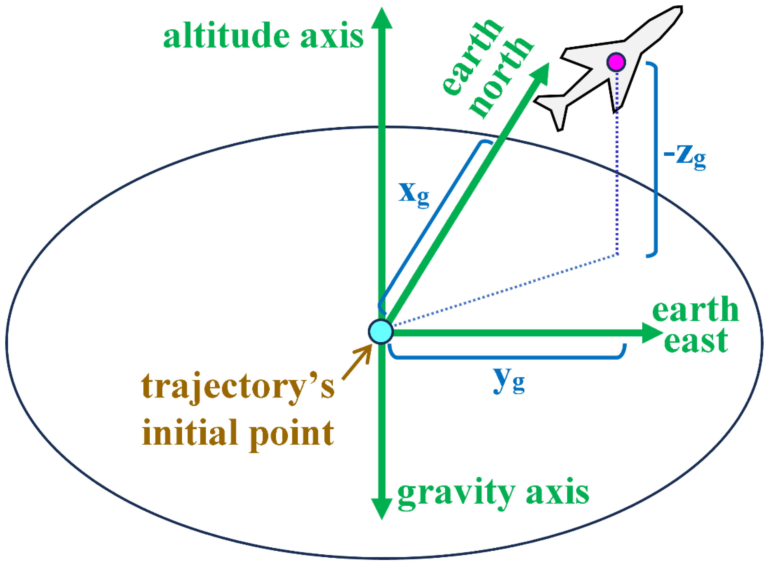
Figure 2.
Illustration of the bank (roll) angle.
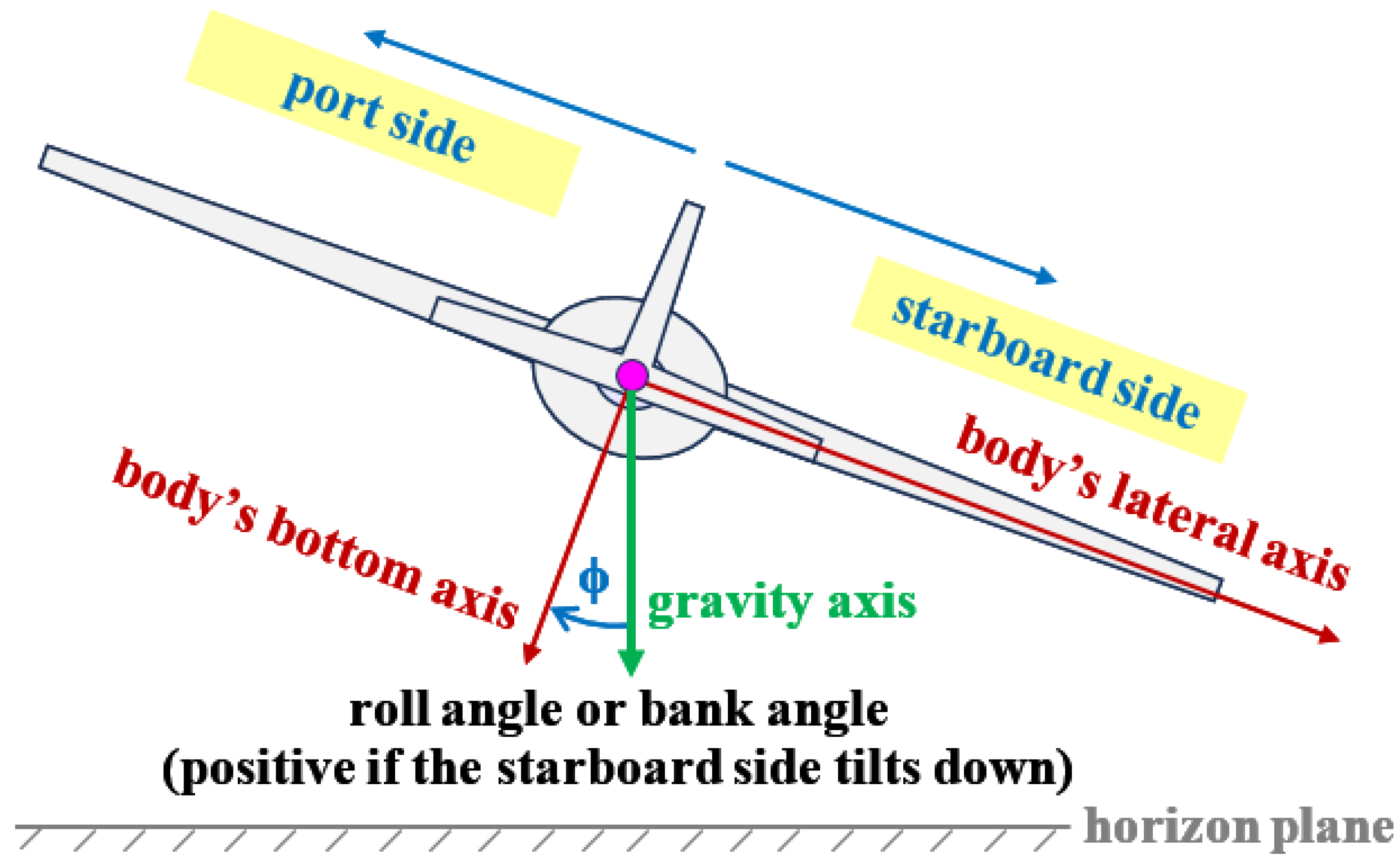
Figure 3.
Illustration of the four flight controls.
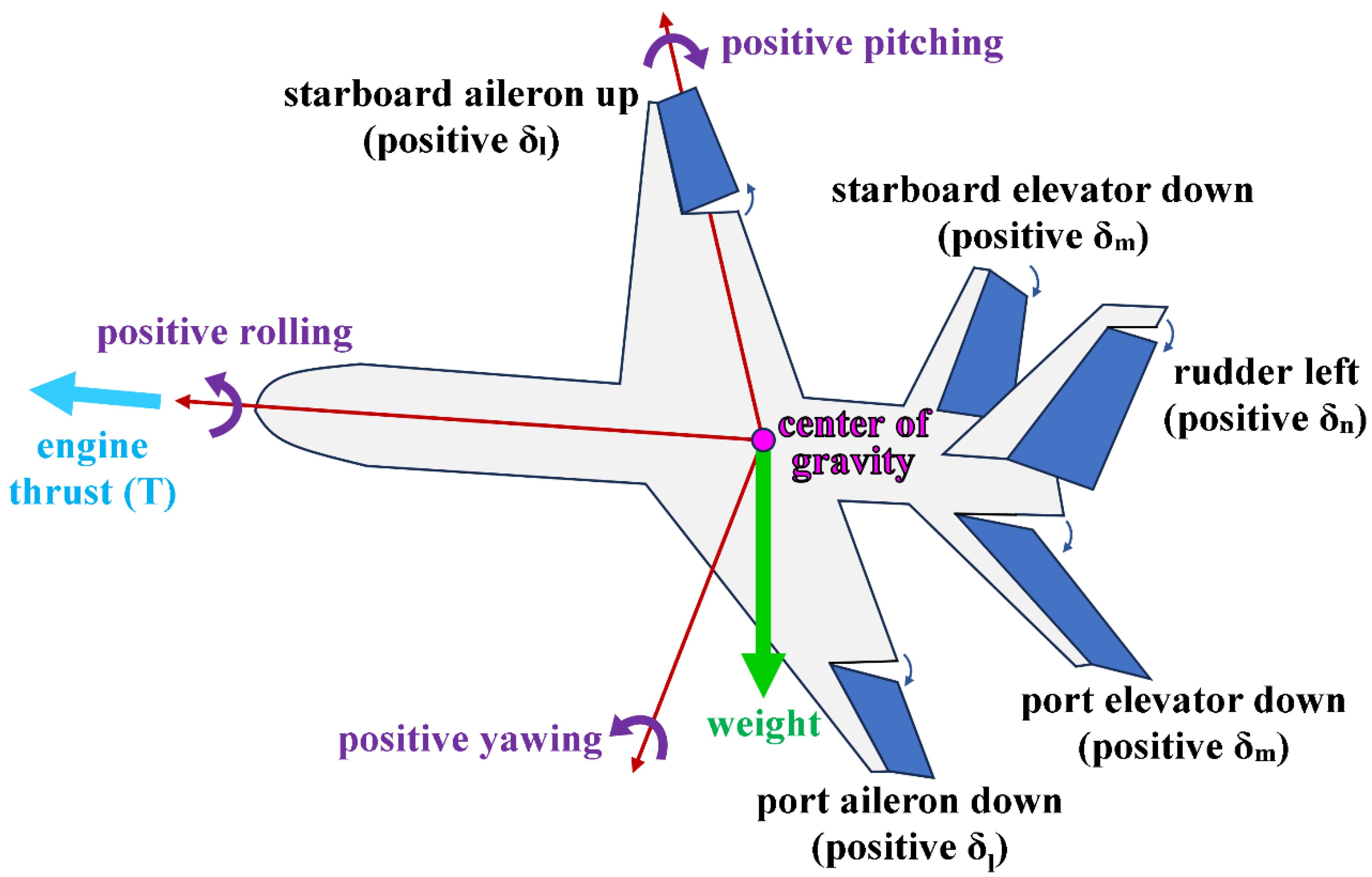
Figure 4.
Illustration of the three Euler angles, as well as the inertial axes and the body axes.
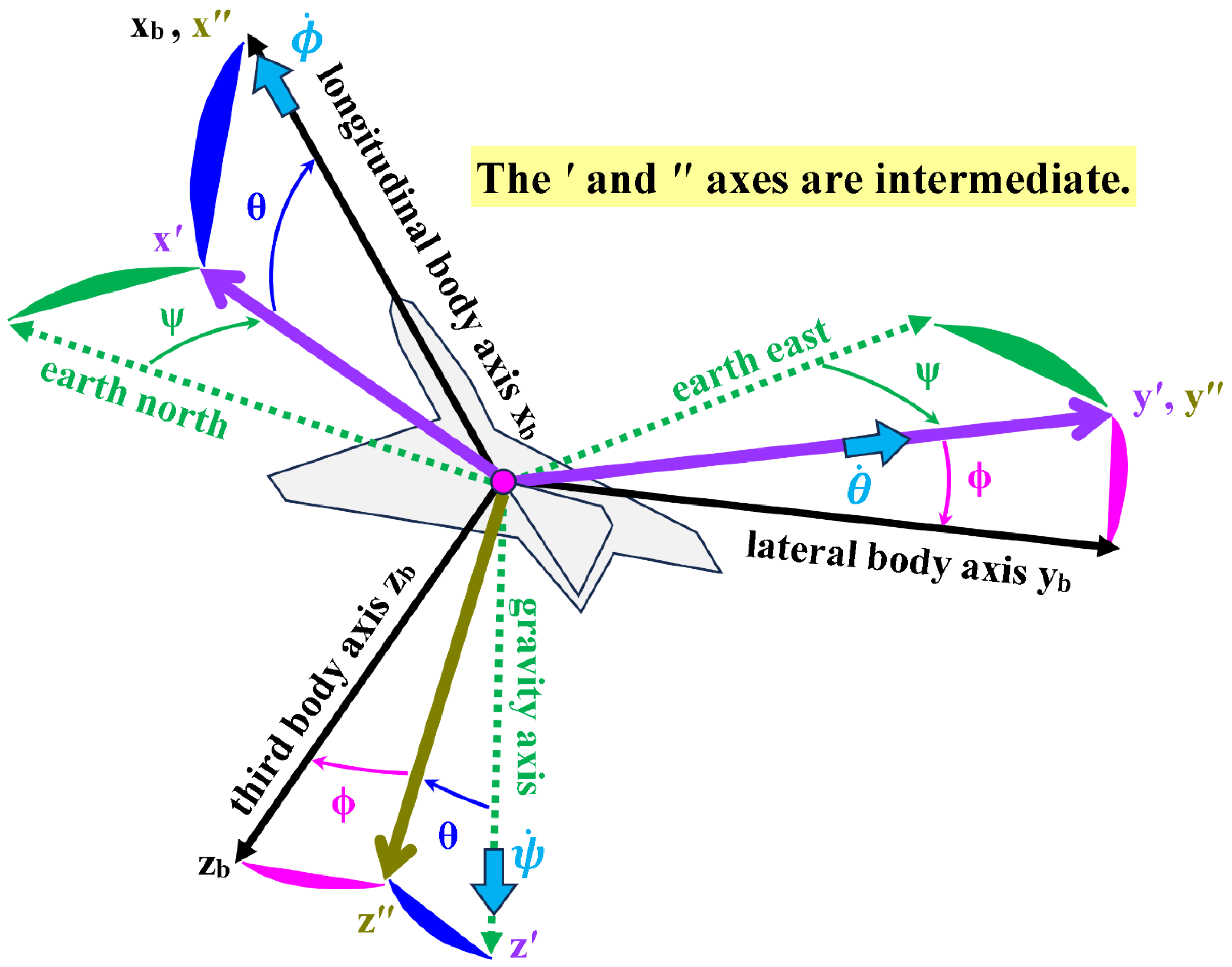
Figure 5.
Illustration of the wind axes and their angles (sideslip angle and angle of attack).
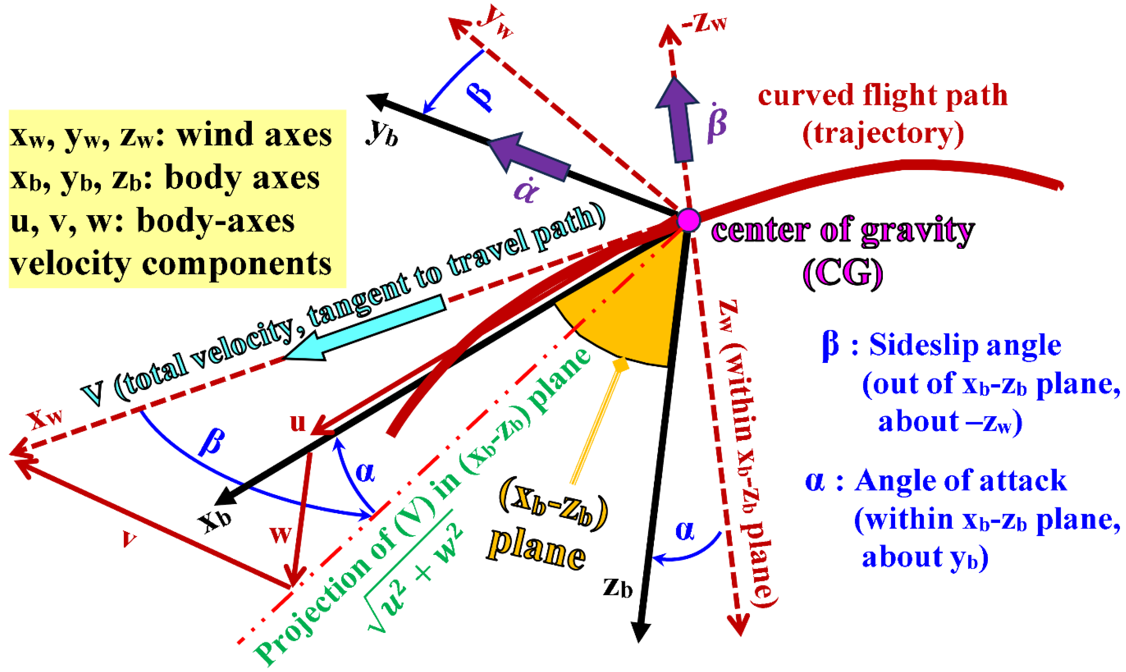
Figure 6.
Illustration of four tilt angles in the midplane of the airplane.
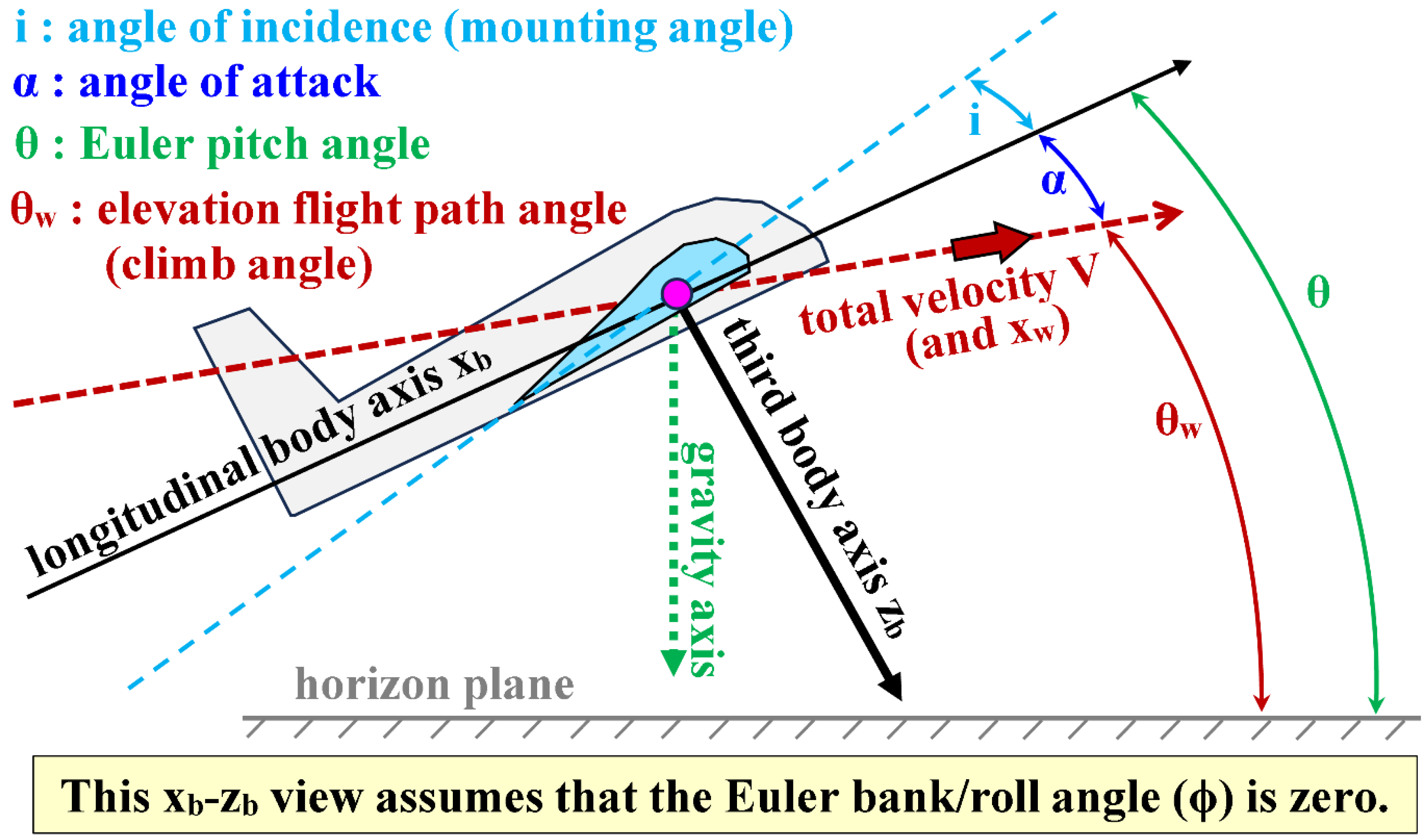
Figure 7.
Illustration of the two flight path angles.
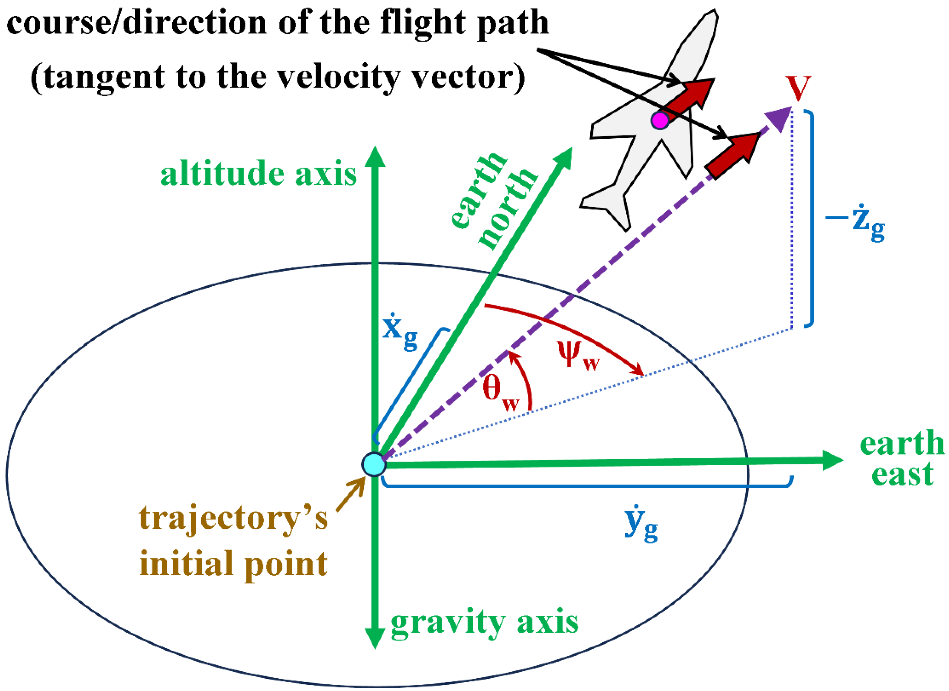
Figure 8.
Illustration of the lift coefficient profile.
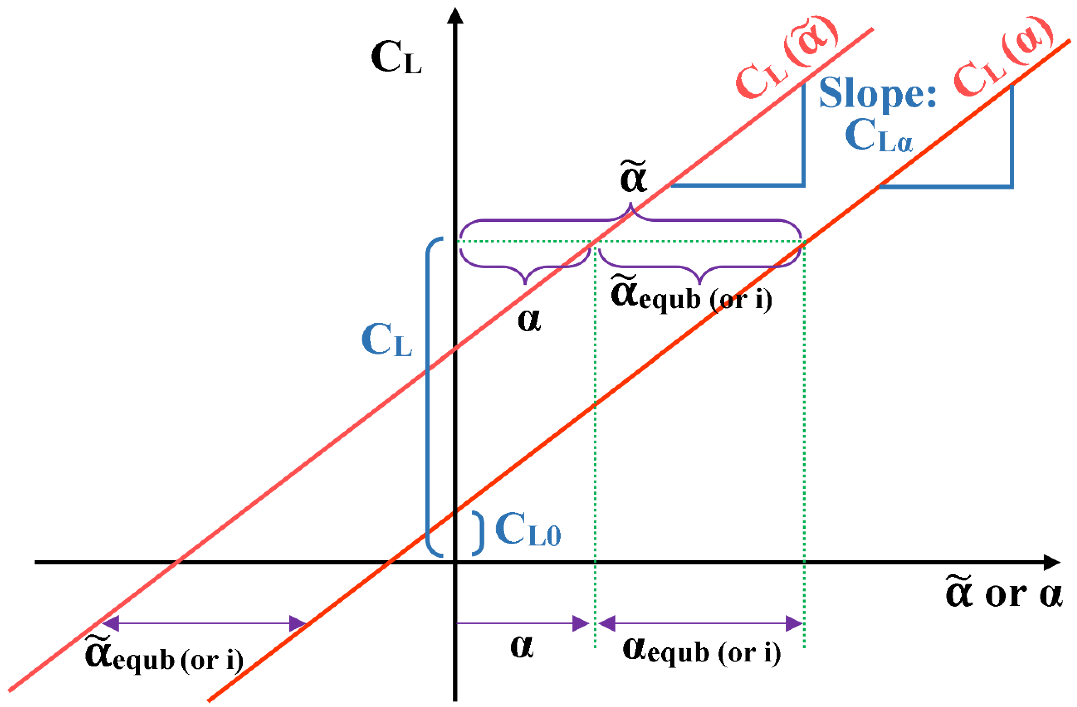
Figure 9.
Illustration of the bank angle profile in the test maneuver.
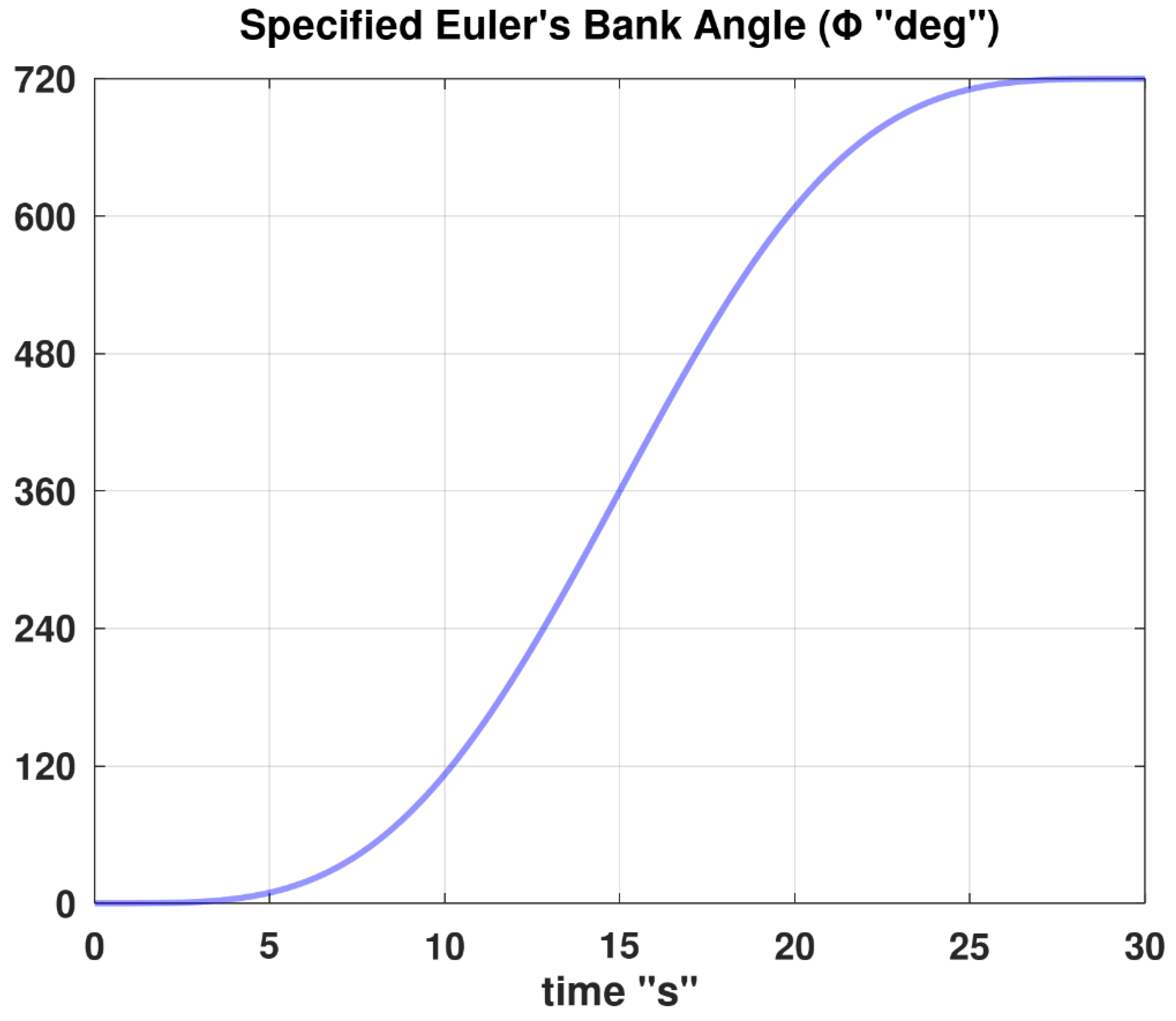
Figure 10.
Illustration of the first derivative profile of the bank angle in the test maneuver.
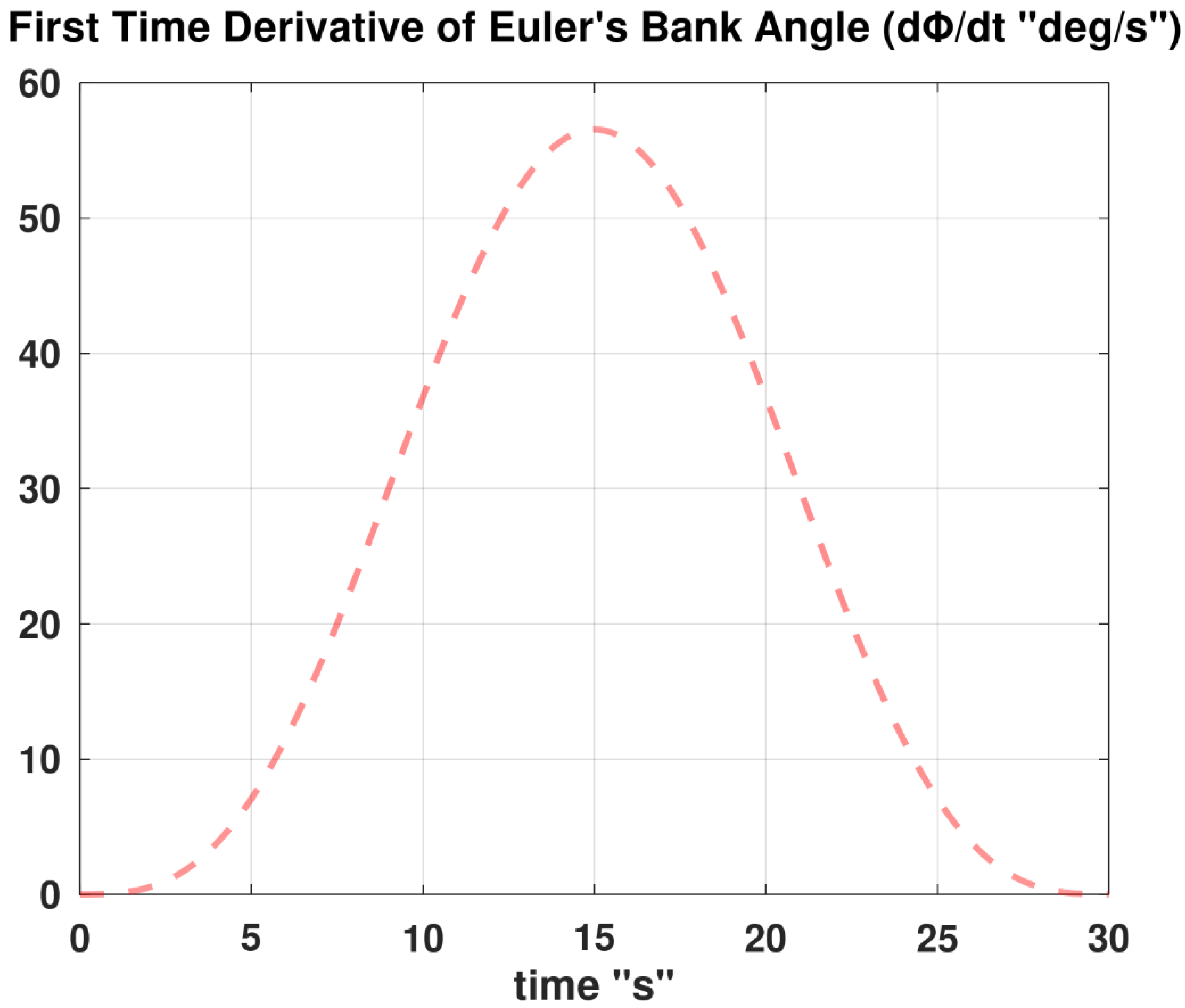
Figure 11.
Illustration of the second derivative profile of the bank angle in the test maneuver.
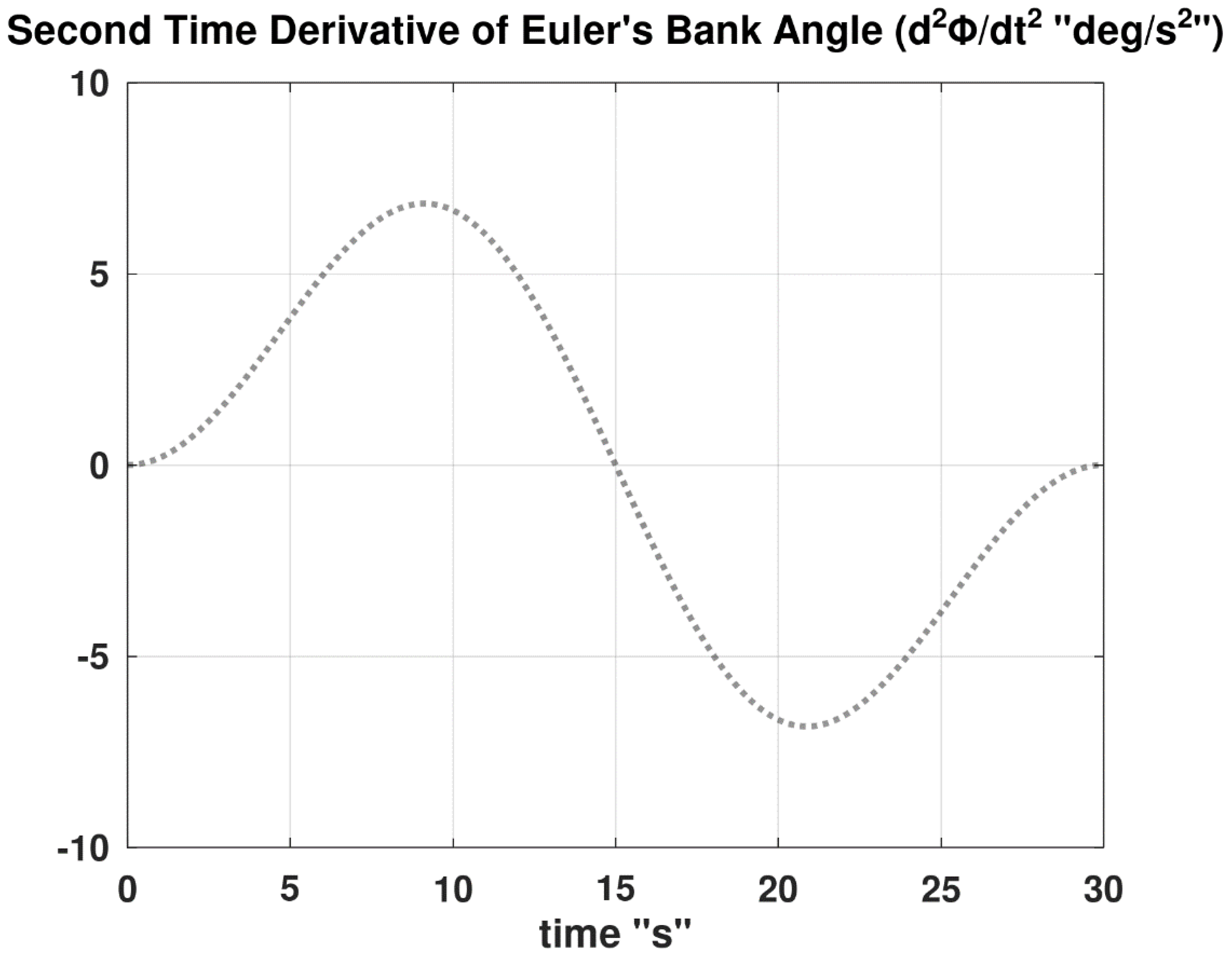
Figure 12.
Computed temporal profile of the thrust flight control during the test maneuver.
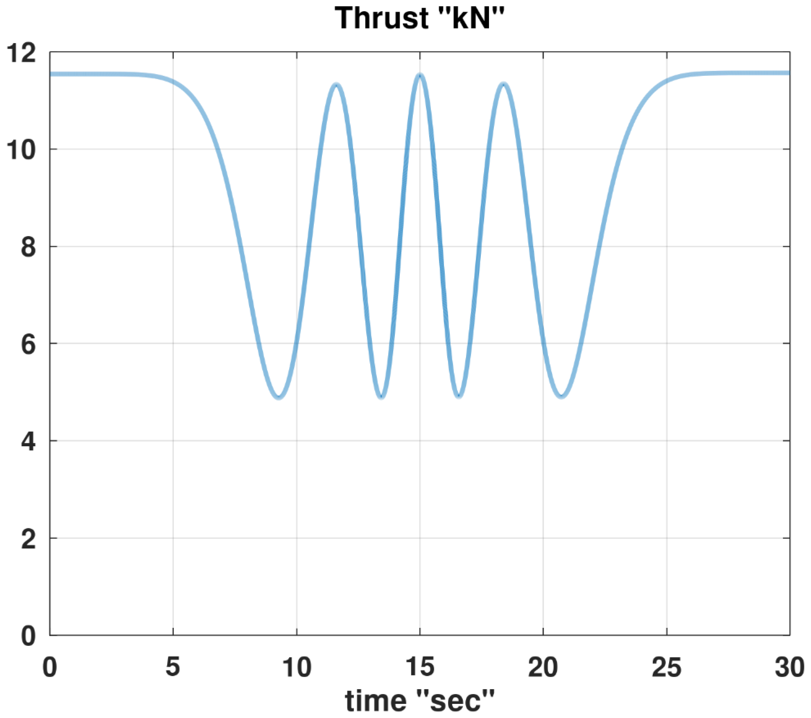
Figure 13.
Computed temporal profile of the rudder flight control during the test maneuver.
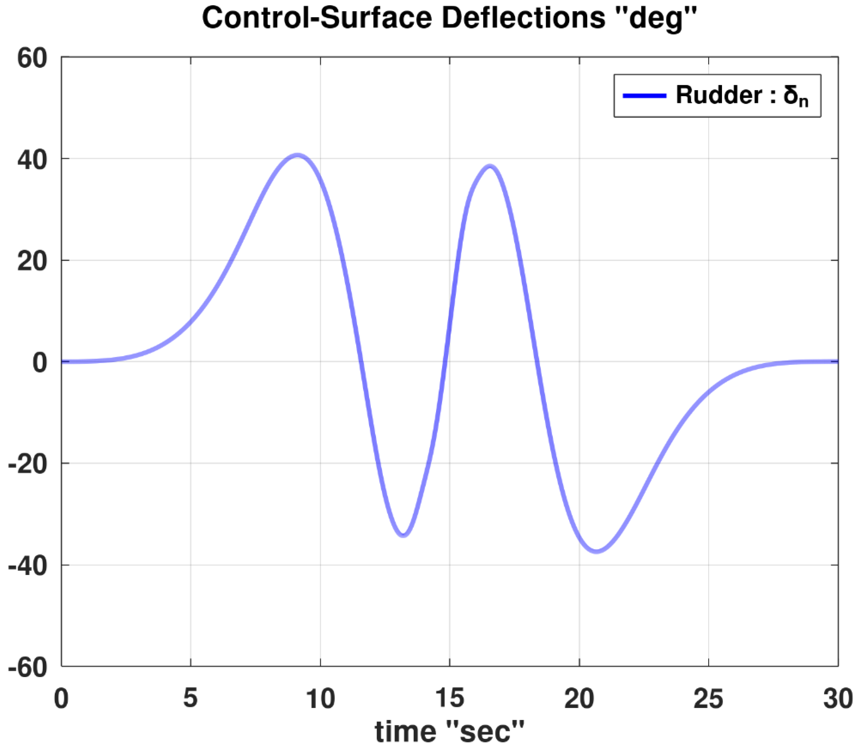
Figure 14.
Computed temporal profiles of the elevators and ailerons flight controls during the test maneuver.
Figure 14.
Computed temporal profiles of the elevators and ailerons flight controls during the test maneuver.
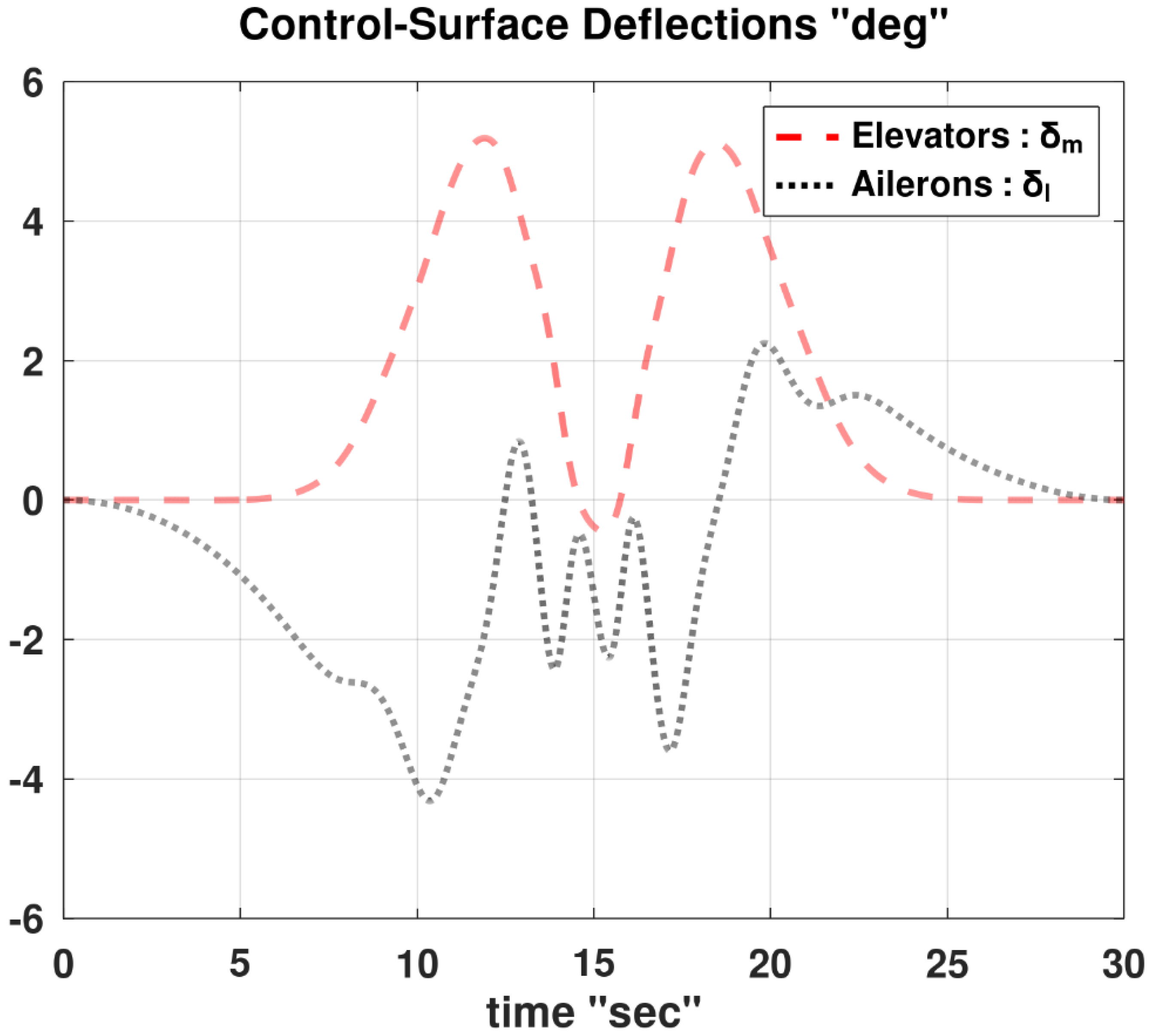
Figure 15.
Computed temporal profiles of the angle of attack and sideslip angle during the test maneuver.
Figure 15.
Computed temporal profiles of the angle of attack and sideslip angle during the test maneuver.
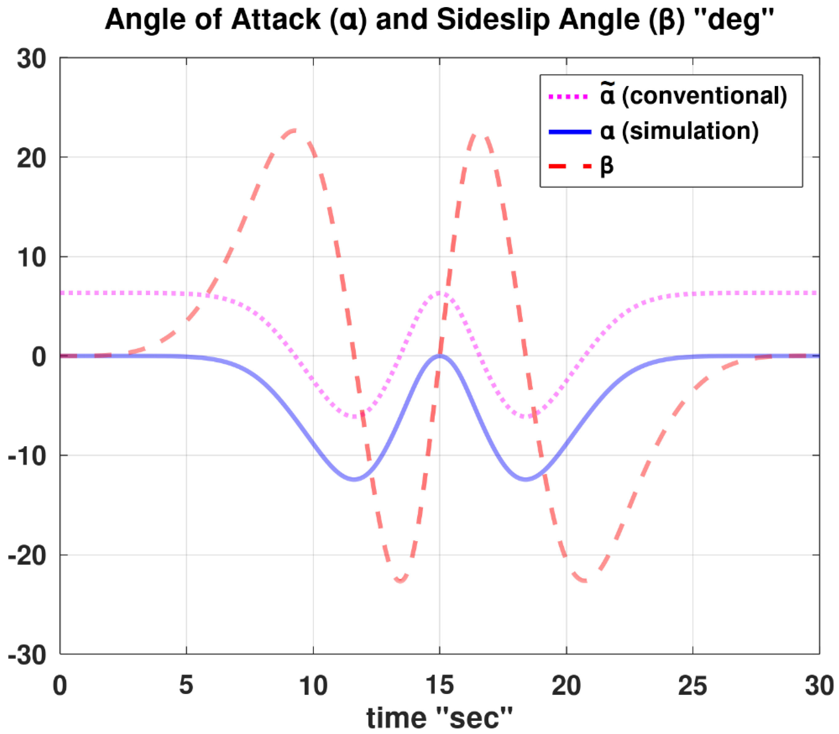
Figure 16.
Computed temporal profiles of the pitch and yaw angles during the test maneuver.
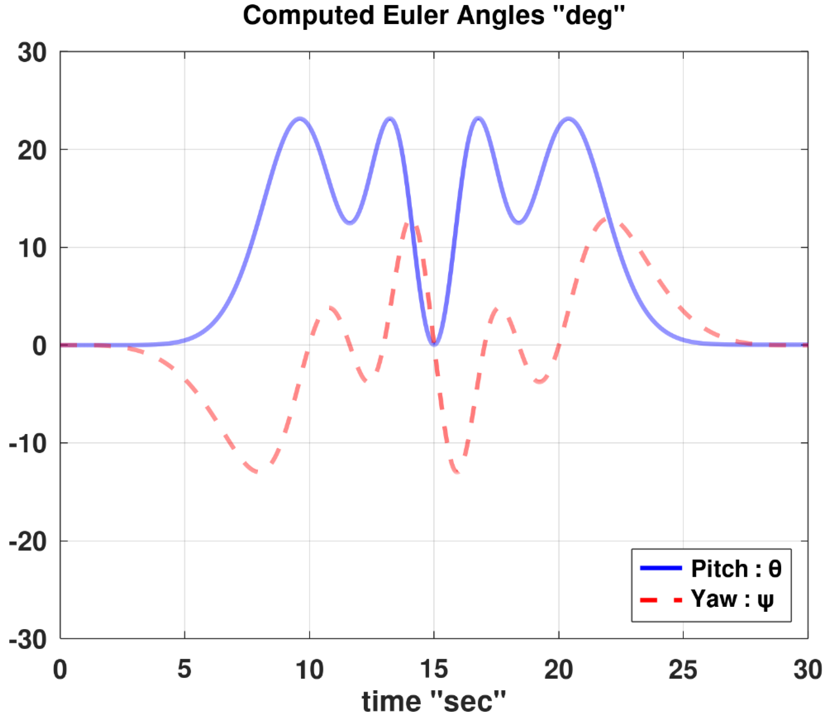
Figure 17.
Computed orbit plot of the pitch and yaw angles during the test maneuver at the used time step of 0.001 s.
Figure 17.
Computed orbit plot of the pitch and yaw angles during the test maneuver at the used time step of 0.001 s.
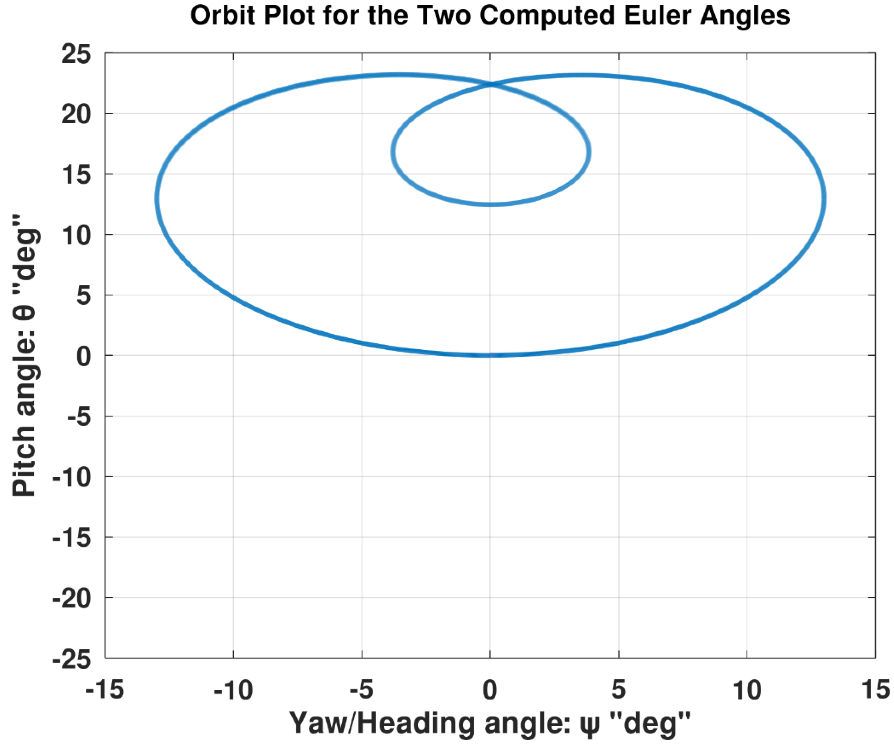
Figure 18.
Computed orbit plot of the pitch and yaw angles during the test maneuver at a coarse time step of 0.01 s.
Figure 18.
Computed orbit plot of the pitch and yaw angles during the test maneuver at a coarse time step of 0.01 s.
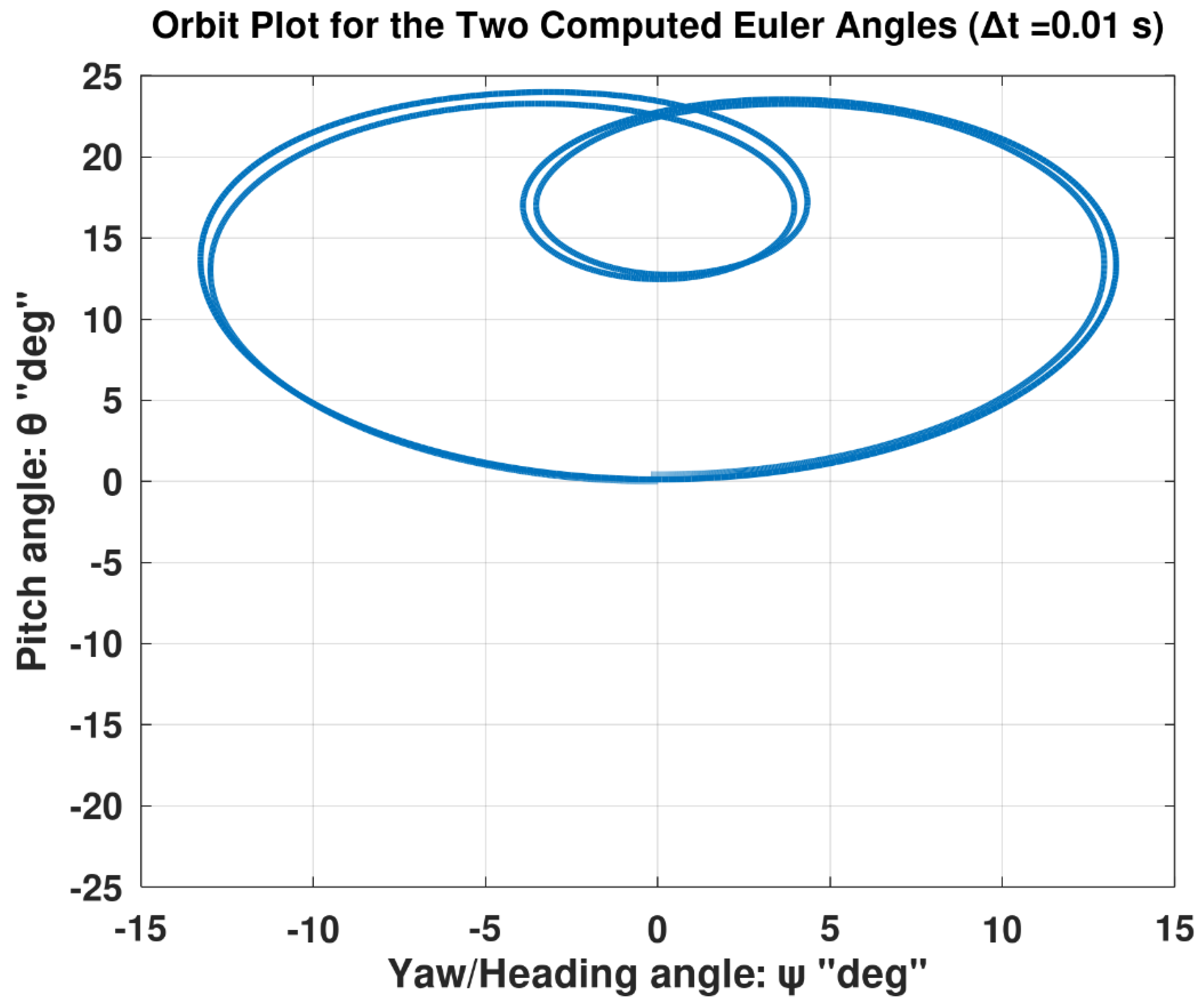
Figure 19.
Computed orbit plot of the pitch and yaw angles during the test maneuver at a coarser time step of 0.02 s.
Figure 19.
Computed orbit plot of the pitch and yaw angles during the test maneuver at a coarser time step of 0.02 s.
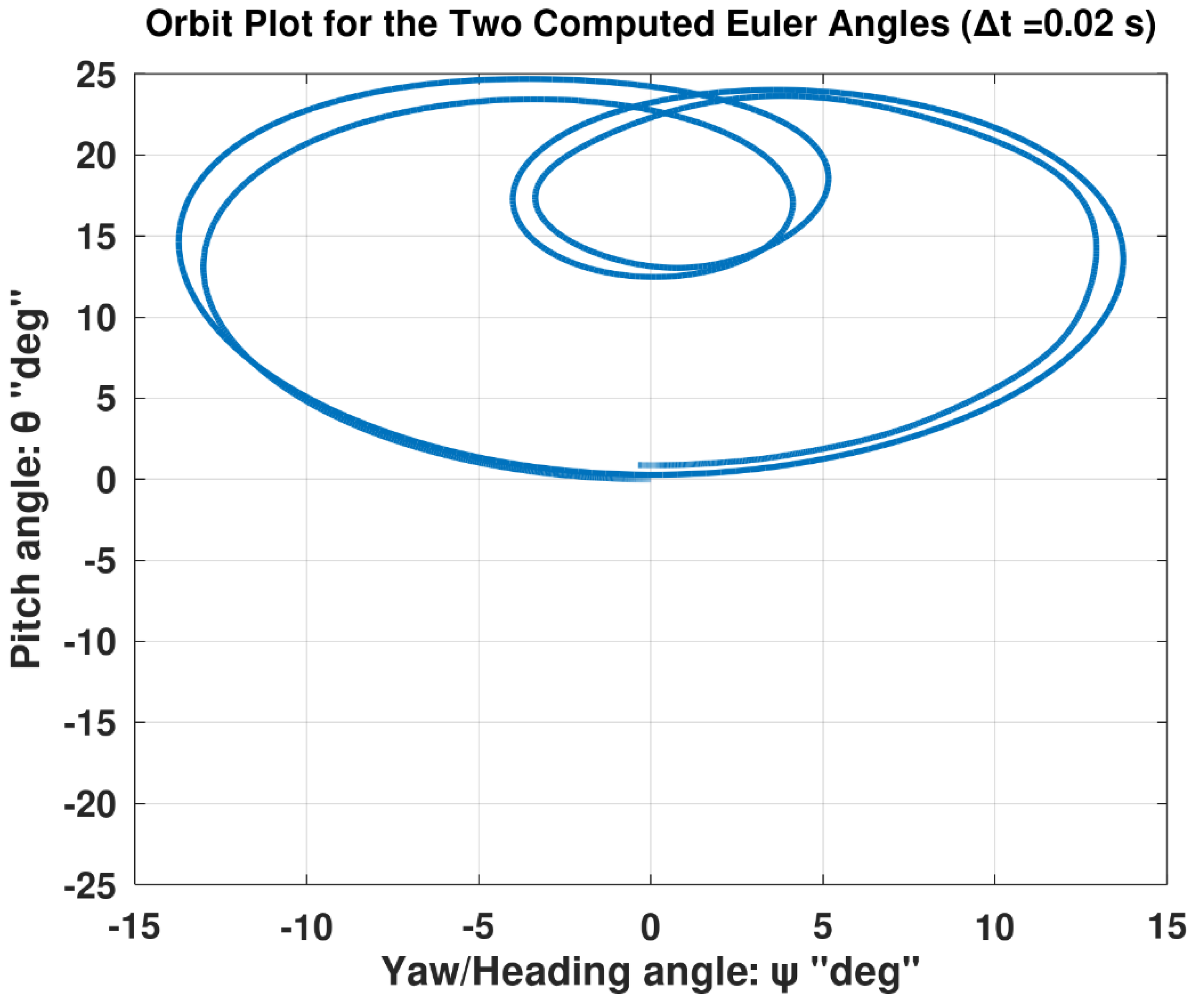

Table 1.
List of the six independent components in the airplane’s symmetric inertia tensor.
| Inertia symbol | Alternative symbol | Meaning |
|---|---|---|
| A | Body-referenced moment of inertia about the longitudinal axis () | |
| B | Body-referenced moment of inertia about the lateral axis () | |
| C | Body-referenced moment of inertia about the bottom/third axis ( ) | |
| D | ) | |
| E | ) | |
| F | ) |
Table 2.
Examples of the geometric and geopotential altitudes within the stratosphere layer.
| Geometric altitude (m) | Geopotential altitude (m) | Absolute difference (m) | Percentage deviation |
|---|---|---|---|
| 5,000.000 | 4,996.079 | 3.921 | 0.0785% |
| 5,003.927 | 5,000.000 | 3.927 | 0.0785% |
| 10,000.000 | 9,984.328 | 15.672 | 0.1568% |
| 10,015.721 | 10,000.000 | 15.721 | 0.1571% |
Table 3.
Quantification of the error in air density calculation at altitudes near 5,000 m.
| Air density computed using an altitude of 4,996 m () | 0.736191 kg/m3 |
| Air density computed using an altitude of 5,000 m () | 0.735872 kg/m3 |
| Air density computed using an altitude of 5,004 m () | 0.735553 kg/m3 |
| 0.0433% | |
| –0.0433% |
Table 4.
Quantification of the error in air density calculation at altitudes near 10,000 m.
| Air density computed using an altitude of 9,984 m () | 0.413234 kg/m3 |
| Air density computed using an altitude of 10,000 m () | 0.412415 kg/m3 |
| Air density computed using an altitude of 10,016 m () | 0.411597 kg/m3 |
| 0.1986% | |
| –0.1983% |
Table 5.
Summary of the 35 flight mechanics equations in the current study.
| Equations group | Equations count |
|---|---|
| Body-fixed axes angular velocity components | 3 |
| Wind-axes linear-momentum equations (and the dynamic pressure) | 4 |
| Body-axes a ngular-momentum equations (including the auxiliary moments) | 6 |
| Inertial velocity components | 3 |
| Flight path angles | 2 |
| Body-fixed axes aerodynamic forces | 3 |
| Body-fixed axes total moments | 3 |
| Aerodynamic and stability (moment) coefficients | 9 |
| Air density (and the flight altitude) | 2 |
| Total | 35 |
Table 6.
Summary of the 39 flight mechanics variables in the current study.
| Variables group | Variables Type (in InvSim) | Variables symbols | Variables count |
|---|---|---|---|
| Inertial coordinates and bank Euler angle | input | 4 | |
| Pitch and yaw Euler angles | intermediate | 2 | |
| Body-axes angular velocity components | intermediate | 3 | |
| Wind-axes coordinates for the linear velocity | intermediate | 3 | |
| Spherical angular coordinates (flight path angles) for the airplane’s inertial location | intermediate | 2 | |
| Body-axes aerodynamic forces (and dynamic pressure) | intermediate | 4 | |
| Body-axes total moments (and auxiliary moments) | intermediate | 6 | |
| Aerodynamic and stability coefficients | intermediate | 9 | |
| Air density and flight altitude | intermediate | 2 | |
| Flight controls | output | 4 | |
| Total | 39 | ||
Table 7.
Summary of the 30 constant parameters for the presented inverse simulation model.
| Parameters group | Parameters symbols | Parameters count |
|---|---|---|
| Airplane mass | 1 | |
| Wing planform (projected) area | 1 | |
| Reference longitudinal length, such as the mean chord | 1 | |
| Reference lateral/directional length, such as the wing span | 1 | |
| Mass moments and products of inertia about body axes | 6 | |
| Aerodynamic-force constants | 5 | |
| Longitudinal stability derivatives | 4 | |
| Lateral stability derivatives | 5 | |
| Directional stability derivatives | 5 | |
| Initial altitude | 1 | |
| Total | 30 | |
Table 7.
General finite difference formulas for numerical differentiation.
| Derivative | Difference type | Expression |
|---|---|---|
| Forward | ||
| Central | ||
| Backward | ||
| Forward | ||
| Central | ||
| Backward | ||
| Forward | ||
| Central | ||
| Backward |
Table 8.
Adopted geometric parameters for Mirage III.
| Serial number | Parameter | Value |
|---|---|---|
| 1 | Mass ( ) | 7,400 kg |
| 2 | Wing planform area ( ) | 36 m2 |
| 3 | Characteristic longitudinal length ( ) | 5.25 m |
| 4 | Characteristic lateral length ( ) | 5.25 m |
| 5 | Moment of inertia about ( ) | 90,000 kg.m2 |
| 6 | Moment of inertia about ( ) | 54,000 kg.m2 |
| 7 | Moment of inertia about ( ) | 60,000 kg.m2 |
| 8 | Moment of inertia in ( ) | 0 kg.m2 |
| 9 | Moment of inertia in ( ) | 1,800 kg.m2 |
| 10 | Moment of inertia in ( ) | 0 kg.m2 |
| 11 | Lift coefficient at zero conventional angle of attack ( ) | 0 |
| 12 | Slope of lift coefficient ( ) | 2.204 1/rad |
| 13 | Drag coefficient at zero lift ( ) | 0.015 |
| 14 | Drag polar parameter ( ) | 0.4 |
| 15 | Side-force coefficient parameter ( ) | –0.6 1/rad |
| 16 | Longitudinal stability parameter ( ) | 0 |
| 17 | Longitudinal stability parameter ( ) | –0.17 |
| 18 | Longitudinal stability parameter ( ) | –0.4 |
| 19 | Longitudinal stability parameter ( ) | –0.45 1/rad |
| 20 | Lateral stability parameter ( ) | –0.05 1/rad |
| 21 | Lateral stability parameter ( ) | –0.25 |
| 22 | Lateral stability parameter ( ) | 0.06 |
| 23 | Lateral stability parameter ( ) | –0.3 |
| 24 | Lateral stability parameter ( ) | 0.018 1/rad |
| 25 | Directional stability parameter ( ) | 0.15 1/rad |
| 26 | Directional stability parameter ( ) | 0.055 |
| 27 | Directional stability parameter ( ) | –0.7 |
| 28 | Directional stability parameter ( ) | 0 |
| 29 | Directional stability parameter ( ) | –0.085 1/rad |
Table 9.
Characteristics of the proposed test maneuver of the Mirage III airplane.
| Serial number | Fixed-value variable | Value |
|---|---|---|
| 1 | Flight speed ( ) |
150 m/s (540 km/h, 291.577 knots) |
| 2 | Azimuth flight path angle ( ) | 0° |
| 3 | Elevation flight path angle ( ) | 0° |
| 4 | Altitude ( ) |
5,000 m (16,404 ft; 3.1069 mi) |
| 5 | Air density ( ) | 0.73587 kg/m3 |
| 6 | Dynamic pressure ( ) | 8,278.56 Pa |
| 7 | Air absolute temperature ( ) | 255.65 K (–17.50 °C) |
| 8 | Air absolute pressure ( ) | 53,992 Pa (0.53286 atm) |
| 9 | Speed of sound in air ( ) |
320.50 m/s (1,153.8 km/h ; 623.00 knots) |
| 10 | Mach number ( ) | 0.4680 |
| 11 | Equilibrium conventional angle of attack ( ) | 6.3322° |
Disclaimer/Publisher’s Note: The statements, opinions and data contained in all publications are solely those of the individual author(s) and contributor(s) and not of MDPI and/or the editor(s). MDPI and/or the editor(s) disclaim responsibility for any injury to people or property resulting from any ideas, methods, instructions or products referred to in the content. |
© 2025 by the authors. Licensee MDPI, Basel, Switzerland. This article is an open access article distributed under the terms and conditions of the Creative Commons Attribution (CC BY) license (http://creativecommons.org/licenses/by/4.0/).
Copyright: This open access article is published under a Creative Commons CC BY 4.0 license, which permit the free download, distribution, and reuse, provided that the author and preprint are cited in any reuse.


