
Submitted:
14 June 2025
Posted:
17 June 2025
You are already at the latest version
Abstract
A previous analysis of Antarctic acoustic data relevant to quantifying frazil contributions to sea ice accretion is reconsidered to address inconsistencies with river frazil results acquired with similar instrumentation but augmented to suppress instrument icing. It was found that sound attenuation by consequent icing limited credible Antarctic acoustic frazil measurements to afternoon and early evening periods which are show to encompass daily minimums in frazil production. This reality was masked by use of an unvalidated liquid oblate spheroidal frazil characterization model which greatly overestimated frazil concentrations. Much lower frazil contents were derived for these periods using a robust 2-frequency characterization algorithm which incorporated a validated, alternative, theory of scattering by elastic solid spheres. Physical arguments based on these results and instrument depth data were strongly suggestive of maximal but, currently, unquantified frazil presences during unanalyzed heavily-iced late evening and morning time periods.
Keywords:
acoustic backscattering
; frazil
; sea ice
; Antarctic sea ice
; river frazil
; in situ ice growth
Key Points
- Accurate Antarctic backscattering measurements with unwarmed instruments were limited to periods of minimal icing and low frazil content
- Accurate frazil characterization requires algorithms compatible with measured backscattering data and ice’s elastic solid rheology
- Valid Icing-free period characterizations and data on instrument depth and backscattering strength imply maximal evening/morning frazil growth
1. Introduction
Frazil ice is a potentially significant factor in the growth and stability of Antarctic coastal sea ice. To date, quantitative data relevant to modelling underlying suspended frazil populations have been restricted to characterizations derived from acoustic backscattering data (Frazer et al., 2020) acquired from landfast ice in McMurdo Sound (MS) offshore of the McMurdo Ice Shelf (Figure 1a). This work utilized a methodology similar to one applied in river frazil studies (Marko & Jasek, 2010a,b: Ghobrial et al., 2012; Marko et al., 2015). However, the MS studies did not incorporate critical flows of heated water adjacent to acoustic sensors and relied upon a new and untested frazil characterization algorithm (Kungl et al., 2020). The heated water flows had previously (Marko et al., 2015) been found essential for suppressing in situ ice growth on and near sensors in the Peace River (PR). Acoustic signal attenuation by this growth was observed to preclude accurate estimates of frazil fractional volumes, F, and other parameters descriptive of frazil populations in turbulent river environments.
Concerns regarding the impacts of these differences in methodology were first raised by apparent inconsistencies between respective river- and Antarctic-ratios of measured volume backscattering coefficients (sV and SV ≡ 10logsV) relative to accompanying estimates of frazil fractional volume. Additionally, unusual correlations between measured SV values and diurnal environmental changes motivated basic reviews and evaluations of the utilized measurement and interpretative methodologies.
Such efforts begin below with an outline of the Frazer et al. (2020) acoustic backscattering (AB) study procedures and their relationship to those used in earlier river work. Key Antarctic and Peace River study results are assembled and used to identify significant anomalies and/or incompatibilities relative to both each other and theoretical expectations. The centrality of river results in interpreting and understanding Antarctic marine backscattering data necessitates references to an included description of AB data collection during a typical Peace River frazil event.
The importance of the frazil fractional volume parameter in all interpretations required critical reviews of the Kungl et al. (2020) frazil characterization algorithm. This review utilized an expanded version of a 2-frequency characterization approach (Marko & Jasek, 2010b) which provides a general tool for assessing feasibilities of deriving convergent optimal frazil characterizations on any given set of SV data. This potentially self-validating approach is applied to the analyzed Frazer et al. (2020) data in conjunction with both the Kungl et al. (2020) characterization algorithm as well as with a partially validated (Marko & Topham, 2015) analytic theory (Faran, 1951) of river frazil backscattering by elastic ice spheres. These results provide the principal basis for reassessing and updating MS frazil production estimates during the 12:00 to 00:00 local time periods typically spanned by Frazer et al. (2020) analyses. The temporal bias of the MS data processing prioritized needs for obtaining additional physical understandings from river data and unanalyzed portions of the Frazer et al. acoustic and oceanographic data sets. Such efforts provide rough characterizations and projections of frazil production during critical portions of daily cycles. The implications of these results are discussed relative to both frazil’s importance in sea ice models and requirements for obtaining more definitive knowledge of frazil production in proximity to ice shelve edges.
2. Methods and Data
The data utilized in this work were primarily extracted from archived compilations (Robinson et al., 2020) of 2017 Frazer et al. (2020) acoustic field data. Additional information essential for new analyses and interpretations of key data features were drawn from a large body of similar AB studies (Marko et al., 2015; Marko & Topham, 2021) carried out in the Peace River. Focus is given to explication of anomalies in the Frazer et al. results relative to general understandings of marine frazil environments and a relevant body of river frazil acoustic results. After a brief summary of basic elements of the Frazer et al. measurements and interpretations, including noting important distinctions relative to cited river studies, the present Section concentrates on key anomalous features of the reported results. Correlations are identified linking these features to both ignored ancillary data and to comparable aspects of Peace River frazil results. The strength and utility of the latter connections were sufficient to necessitate a brief graphical presentation of AB data acquired during a typical river frazil growth event as a guide for subsequent interpretations and re-analyses of the Frazer et al. results.
2.1. Basic Elements of the Frazer et al. Study
The Frazer et al. (2020) field studies were carried out in November, 2016 and 2017 at MS locations 33 and 13 km, respectively, north of the McMurdo ice shelf (Figure 1a). Each field program acquired 2 weeks of data from a suspended upward-looking AZFP (Acoustic Zooplankton Fish Profiler) instrument manufactured by ASL Environmental Sciences Inc. Measurements utilized AB signal returns from acoustic pulses emitted at 1 Hz at each of four different frequencies (125, 200, 455 and 769 kHz) (referenced as channels 1 through 4, respectively). Instruments were initially positioned 30 m below the sea ice undersurface. SV values were computed from detected signal voltages and instrument and measurement parameters using an ASL Matlab Toolbox (Version 1.1). Frazil properties were characterized for 11 minute-averages of SV(t) values obtained after averaging over five 0.1 m deep measurement cells (Robinson et al., 2020).
Procedures developed in earlier, suspended sediment- and zooplankton-related, AB studies (Hay & Sheng, 1992; Stanton et al., 1998) were used to quantify lognormal distributions of a representative particle dimension which, in the Frazer et al. (2020) work, was a spheroid diameter. Distribution parameters, established by optimal matching of measured SV values to theoretical counterparts, supported fractional volume estimates. Matching required achieving equalities between measured- and theoretical-backscattering cross sections, σBS (imaginary areas representing fractions of acoustic power intensity incident upon a unit volume which is scattered back toward the power source). The Frazer et al. work utilized a new, unvalidated, theoretical cross section relationship (Kungl et al., 2020) which treated frazil particles as liquid oblate spheroids. This choice represented a significant deviation from river frazil characterization procedures (Marko et al., 2015) which utilized theoretical cross sections specific to elastic solid ice spheres (Faran, 1951,).
Although prior studies (Pietrovich, 1956; Marko et al., 2015; Marko & Topham, 2021) suggested that water sufficiently supercooled for frazil crystallization supported simultaneous in situ ice growth on submerged surfaces, Frazer et al. (2020) adjustments for observed apparatus icings were limited to a Nov. 9-10 sequence of instrument-recovery, -de-icing and -redeployment actions. This sequence was initiated by sudden onsets of decreases in instrument depth which began to severely degrade SV data roughly 2.5 days after each of two successive 2017 instrument deployments.
2.2. Potential Data Anomalies
Although archived digital data (Robinson et al., 2020) provided the principal basis for our evaluations, possibilities for anomalously weak backscattering were first raised by the extremely low time-averaged 17:59 NZST (Z +12 h) Nov. 11, 2017 SV values plotted in Frazer et al.’s (2020) Figure 1b. The weakness of detected returns is evident in our Figure 1b which replots the Frazer et al. 15 m SV frequency dependences alongside SV results acquired 2.6 m above the riverbed during a typical Peace River frazil event (Marko & Topham, 2015, 2021). Given large differences in measurement locations, depths and, possibly, crystallization mechanisms (Daly, 1984; Lewis & Perkin, 1986, 1987; Smedsrud & Jenkins, 2004), the 15 to 25 dB depressions of Frazer et al. (2020) SV values relative to PR estimates at similar frequencies was only recognized as problematic after comparisons of contemporary MS and PR F(t) results. Specifically, peak F values associated with the PR data (Marko & Topham, 2015, 2021) were barely 5 times (7dB) larger than the 1x10⁻⁵ 15 m values indicated in Frazer et al.’s (2020) Figure 4e for the Antarctic time interval. This result was incompatible with the 400-fold discrepancies anticipated from the rough proportionalities of contemporary F and SV values dictated by their common linear theoretical dependences on volumetric particle number density. Such an inconsistency was suggestive of either large differences in the intrinsic scattering strengths of, respectively, MS- and PR-frazil species or major deficiencies in one or both algorithms used to derive F values from SV data.
The latter possibility would have introduced significant problems into Frazer et al.’s (2020) analyses, because of the algorithm’s use for an initial “filtering” of raw data. This step was intended to assure “physically plausible” results by avoiding characterizations of weak returns from extraordinarily high numbers of very small particles. Consequently, all profiles with 200 kHz SV values below -85 dB were excluded from frazil fractional volume estimates. Time periods associated with the eliminated data, comprising, roughly, 40% of recorded profiles, are denoted by horizontal red lines in Figure 1c which plots Frazer et al. (2020) MS SV data as functions of time and frequency. The SV plots, which, for readability purposes, used indicated subtractions to effect frequency-specific offsets, represented Nov. 10-13, 2017 data acquired at 14.2 m depths. Shading of 00:00–12:00 NZST periods (designated as “prenoon” intervals) demonstrates the nearly complete confinement of unprocessed Frazer et al. (2020) data to these portions of the diurnal cycle. Importantly, SV data acquired in these periods also exhibit consistent distinctions relative to corresponding processed 12:00-00:00 NZST (postnoon) results. Specifically, prenoon SV(t) values were lower in magnitude and marked by greater ranges of variability.
Diurnalities were also a feature of river frazil studies (Marko et al., 2015), albeit with SV and F values being maximal during prenoon as opposed to postnoon periods. It is notable that the latter aspect of river frazil data was only recognized in the presence of active icing deterrence by sensor warming. Without such warming, it is not unreasonable to consider that the low prenoon SV values excluded from Frazer et al. (2020) analyses were consequences of sound attenuation by sensor and apparatus icing which, in rivers, were signatures of high frazil content (Marko & Topham, 2021). This possibility was also consistent with the fact that the 2017 oceanographic results in Frazer et al.’s Figure 4g showed, prenoon periods hosting peak northward inflows of supercooled water from the 13 km distant ice shelf. Similar flows provided a potential basis (Lewis & Perkin, 1985, 1986; Smedsrud & Jenkins, 2004; Hughes et al., 2014) for local Antarctic frazil production by upward movements of buoyant frazil particles.
Figure 1c includes additional, ancillary, data on changes in instrument depth supportive of intensive icing similar to that observed in rivers during prenoon intervals. These data, drawn from Robinson et al. (2020), are displayed for both the Nov. 10-14, 2017 period encompassing the SV data in Figure 1c as well as for an immediately preceding Nov. 5-9, 2017 interval not, otherwise, included in our SV(t) reanalyses. The latter depth changes are plotted relative to a secondary horizontal time axis which is shifted forward by five days to overlap the primary time axis. This shift facilitates displays of depth change commonalities during the two different 2017 acoustic measurement periods. Each interval was marked by 2.5 days of instrument depth stability terminated by sudden and continued depth reductions. SV measurement uncertainties, introduced by these instrument shifts, necessitated the Nov. 9 and subsequent terminal Nov. 14 instrument recoveries.
Both onsets of instability, presumably indicative of accumulated apparatus icing sufficient to achieve neutral buoyancy, occurred at the beginnings of a prenoon interval. Relative depth stabilities were only, temporarily, re-established early in immediately following postnoon periods. This pattern was repeated, on reduced spatial scales, during at least the first half of immediately following diurnal cycles. Such changes suggested that the bulk of icing and likely accompanying frazil production was accumulated during the prenoon intervals eliminated from Frazer et al. (2020) analyses. Similarities between such behavior and the above-noted diurnal river icing patterns were sufficiently striking to justify a brief review of key aspects of AB measurements during a typical river frazil event for further reference in later interpretations of Figure 1c SV data
2.3. Acoustic Backscattering Measurements in Rivers: Relevance to Frazer et al. (2020) Results
Signal attenuation by icing along acoustic trajectories degrades multifrequency frazil characterizations. Information on consequent impacts and avoidance measures is accessible from acoustic data acquired during a typical daily cycle of PR frazil- and in situ-ice growth depicted in the echogram of Figure 1d. These data represent 16-bit 774 kHz backscattered digital signal voltages recorded as functions of time and range to water column targets. Earlier analyses (Marko & Topham, 2021) showed frazil growth during the represented Feb. 7, 2012 period beginning at, roughly, 00:00 MST (Z + 7 h). Coincident in situ growth was initially inferred indirectly through accompanying releases of latent heat which partially suppressed frazil levels below an initial peak value. Direct evidence of such growth appeared seven hours after frazil onset as initial thickening of a ubiquitous red, near-zero range, echogram feature introduced by near-field measurement effects unrelated to frazil presence. The thickening of this feature, designated as “close-in” signal returns, represented backscattering by sensor icing which attenuated outgoing and incoming sound pulses, thereby weakening water column frazil signals. External sensor warming delayed onsets of signal blockage until upper portions of a riverbed ice layer made physical contact with elevated acoustic sensors. Consequent delays in blockage onsets allowed use of the data in Figure 1d to confirm earlier (Ghobrial & Loewen, 2021; Marko & Topham, 2021).) 4 cmh-1 estimates of riverbed ice growth rates.
Continued sensor icing and subsequent thinning produced an 11:30 MST peak in close-in thickness coincident with a consequent minimum in river surface signal voltages. Gradual icing clearances, after 14:30 MST, allowed reappearances of weak water column frazil signals which strengthened into an evening peak preceding 20:00 MST reappearances of detectable close-in regrowth. This regrowth can be seen to have eventually eliminated detection of all water column returns by midnight. The 18:20 and 19:15 MST SV frequency dependence data in Figure 1b corresponded to, respectively, the leading edge and centre of a modest early evening echogram peak. The first of these two returns, which was marginally detectable, was almost 15 dB larger than its coplotted Frazer at al. (2020) counterparts: suggesting the latter would have been undetectable in the noisier PR environment.
Applying river frazil understandings to interpret Frazer et al. (2020) data requires accommodating notable differences in the PR and MS measurement environments. Specifically, the 2017 MS environment did not include large natural features, such as riverbeds, capable of supporting sufficient in situ ice growth to suppress suspended frazil contents. Similar growth on sea ice undersurfaces may have been present but lower water flow speeds and large separations from frazil measurement volumes precluded river-like frazil content impacts (see Section 4). However, without applied warming, signal attenuation by in situ growth on acoustic sensors was a potential source of Frazer et al. (2020 ) frazil content underestimates.
Results in both environments could be expected to be sensitive to prenoon/postnoon differences. In rivers, apart from a short interval following frazil onset, simultaneous frazil- and instrument icing-growth would have confined uncontaminated unwarmed sensor measurements to time windows immediately following frazil onset and during early to- mid-postnoon icing clearances. The lengthy periods of potentially uncontaminated postnoon SV data analyzed in Frazer et al. (2020) could have been taken as evidence for the low icing presences inferred for such periods from contemporary instrument depth stabilities. However, as in the PR observations, the absence of icing growth also may have been indicative of low frazil contents. Clarifying this situation requires resolving uncertainties in the Frazer et al. (2020) characterizations and the underlying Kungl et al. (2020) algorithm. More fundamentally, such clarifications are essential for quantifying and assessing the significance of the SV(t) data in Figure 1c relevant to estimates of overall daily MS frazil production.
3. Analyses
3.1. Evaluations of Frazil Content Estimation Algorithms
Our approach used observed instrument depth stabilities to tentatively justify ignoring icing-related acoustic attenuation during the postnoon periods associated with all Frazer et al. (2020) fractional volume estimates. This choice focused attention on differences between algorithms applied to, respectively, PR and MS data. Both algorithms optimized agreement between theoretical and measured SV values using squared error minimization techniques and SV(t) data usually acquired at three and four frequencies, respectively, in river studies and in the MS work. Ideally, PR optimizations, employing equal numbers of known input- and unknown output-parameters, were fully determined: allowing exact characterizations. However, data and theory imperfections yielded finite root mean square (rms) errors (Marko et al., 2015) as rough indicators of F(t) estimate accuracy. No equivalent Frazer et al. (2020) error measures were available for similar evaluations of overdetermined 4-frequency extractions.
In both cases, characterization quality reflected assumed theoretical linkages of backscattering strength to acoustic frequency and parameters defining host fluid and insonified particle properties. PR extractions utilized Faran’s (1951) exact (analytic) formulation of elastic solid ice sphere backscattering cross sections in terms of water and ice mass densities, a particle dimension and fluid and target rheologies. These relationships were verified by laboratory measurements (Marko & Topham, 2015) on polystyrene sphere- and disk-surrogates treated as “effective spheres“ (Ashton, 1986) with “effective radii”, ae, defined to reproduce actual particle volumes. Polystyrene disk results showed small, < 2 dB, errors for frequency combinations, k1ae, exceeding 0.6 where k1 ≡ 2π/λ and λ denotes sound wavelengths in host fluids. Optimal 3-frequency matching to PR frazil data (Marko et al., 2015)) primarily returned average rms SV(t) errors approximating 1 dB in each frequency channel for frazil populations with lognormally distributed ae values and particle number volumetric densities, N. Distribution parameters included a mean effective radius, am, and a width, b, representing the standard deviation of ln(ae).
The complexities of 3- and 4-frequency characterizations reflected, in part, efforts to quantify frazil dimension parameters rarely used as fundamental inputs to ice growth models or operational ice assessments. Frazil shape- and size-variations and their temporal instabilities, combined with dearths of independent, non-acoustic, verification data, greatly complicated realistic particle descriptions. Abandoning spherical particle treatments required poorly documented assumptions to link additional dimension statistics to particle volumes and cross sections.
Reviews of the largest body of characterizations (Marko et al., 2015) showed predominance of zero width (b = 0) distributions: indicative of theoretical and/or measurement errors inhibiting convergence to finite b value solutions. The resulting frazil population characterizations were closely related to those derived (Marko and Jasek, 2010b) from data acquired simultaneously with pairs of different frequencies. This 2-frequency approach characterized frazil in terms of populations of N* identical spheres of radius a* per unit volume. Optimal estimates for a fractional volume parameter, F*, equated to 4πN*(a*)3/3, were obtained if differences in SV values measured with a given frequency pair were theoretically calculable from knowledge of a cross section relationship, σBS, assuming that measured values of sV were equal to N*σBS. In practice, this required that measured pair SV differences fell within the ranges of variability associated with curves representing corresponding theoretical pairwise SV differences as functions of a*.
While convergences to b = 0 solutions precluded 3-frequency characterizations at finite b values, the obtained 2-frequency results offered coarser, but robust, fractional volume estimates. This capability reflected the fact that 3-frequency convergence methods implicitly include 2-frequency calculations for each of the three possible pairings of the three incorporated frequencies. Nevertheless, apart from requiring a valid cross section relationship, individual pair F* estimates are only fully representative of F for narrow distributions of particle dimensions. The consequent degrading of F estimates for non-uniformly sized frazil populations is, however, partially mitigated by averaging over results obtained with multiple frequency pairings. Thus, SV data acquired at 3- and 4-frequencies support 2-frequency F* estimates derived with, respectively, three and six different frequency pairings.
Accuracies of pair-averaged 2-frequency F* estimates were quantified by comparisons with F values for hypothetical elastic solid frazil sphere populations with known probability distribution parameters and particles which individually backscatter sound according to the Faran (1951) cross section relationship. These populations were constructed by using this relationship to calculate SV values at the four acoustic frequencies used by Frazer et al. and assuming: a mean effective radius, am; a width parameter, b, and an arbitrarily selected SV value for an included frequency. The resulting sets of 4-frequency SV data supported exact calculations of F corresponding to the chosen am and b values and a numerical volume density, N, established from these values and the arbitrarily selected SV value. The SV data generated for each population allowed 2-frequency F* estimates for each of the six possible frequency pairings. Averaging over these pairings yielded the values of F*avg/F plotted on the solid curve in Figure 2a as a function of b. The resulting sensitivities to frazil size variability suggest that pair-averaged F* values slightly (≈15%) underestimate F for b < 0.2. Broader distributions can be seen to favor overestimates by as much 50% as b approaches 0.3. a value compatible with the upper limits of reported (McFarlane et al., 2015) distributions of frazil disk diameters. Such overestimates were comparable in magnitude and opposite in sign to the approximately -2 dB underestimates introduced (Marko and Topham, 2021) by using elastic sphere cross sections to represent scattering by frazil disks of identical volume. Fortuitous near-cancellation of these two errors suggests that pair-averaged F* values are roughly representative of corresponding 3-frequency fractional volumes. The low residual errors attained using Faran (1951) cross sections in b = 0 frazil characterizations (Marko et al., 2015) suggest that the uncertainties in F* introduced by possible systematic theoretical cross section imperfections are unlikely to exceed a factor of two.
3.2. Evaluating the Kungl et al., (2020) Characterization Algorithm
The algorithm used in the Frazer et al. (2020) data processing evolved (Kungl et al., 2020) from an earlier theory of scattering by oblate penetrable spheroids (Burke, 1968). It replaced ice’s elastic rheology by a liquid alternative which precluded shear deformations critical to theoretical frequency and ae dependences of backscattering by elastic ice spheres. The impacts of this difference are illustrated in Figure 2b by normalized plots of theoretical backscattering cross sections which were exactly calculable as functions of k1ae for ice spheres characterized by, alternatively, elastic solid- (Faran, 1951) and liquid- (Anderson, 1950) rheologies as specified using the indicated MS saltwater- (Robinson et al., 2020) and ice target-sound speeds. The prominent minimum in the elastic solid curve, confirmed in laboratory measurements (Marko & Topham, 2015), was introduced by and, roughly, proportional to shear stress strength. The third curve depicts the corresponding Kungl et al. (2020) relationship with and without conversion of spheroid diameters, D, into effective radii to facilitate comparisons. This relationship was constructed from two slightly different power law dependences on k1ae separated by a narrow k1ae “transition” regime. As noted by Kungl et al. (2020), these simplifications required additional steps to resolve indeterminacies introduced when matchings of theory and measured data utilize pairs of k1ae values linked to theoretical σBS values by a common power law relationship.
Without access to data on rms errors in matches of theory and data, tests of Kungl et al. (2020) characterization accuracies were carried out in Figure 2c for three ((3,2), (4,2), (4,3)) different pairings of frequency channels. This testing utilized 14.2 m SV data acquired during the Nov 11, 12:06 to 19:59, 2017 period to display differences in logarithmic cross section (ΣBS) values, ∆ΣBS(j,i) ≡ 10 log(σBS(j)/σBS(i)), both as measured and theoretically calculated, for each (j,i) frequency pairing. (Given the above equality between sv and N*σBS, measured logarithmic cross section differences in 2-frequency calculations are numerically equal to corresponding differences in AB-measured SV parameters.) Figure 2c facilitates judgements on optimization feasibility by establishing whether ∆ΣBS(j,i)meas values (arbitrarily positioned along the ae and D axes near minima in similarly colored ∆ΣBS(j,i)theo curves) could intersect such curves. The latter curves, plotted as functions of both ae and D, were derived using the Kungl et al. (2020) cross section relationship (curve C in Figure 2b). Vertical lines and circular markers, respectively, denote the ranges and mean values of pair-wise logarithmic measured cross section differences. The ranges of variability and the means of measured differences (which were 2 to 6 dB below the lowest points on corresponding theoretical curves) were not consistent with the existence of 2-frequency solutions. Given the fundamental role of such solutions in optimizations, these results suggest that 4-frequency Frazer et al. (2020) characterizations were spurious: reflecting either fundamental incompatibilities between the Kungl et al. (2020) cross section relationship and MS SV data and/or the presence of icing-related data contamination.
4. Results
4.1. Recalculated Postnoon Frazil Fractional Volumes
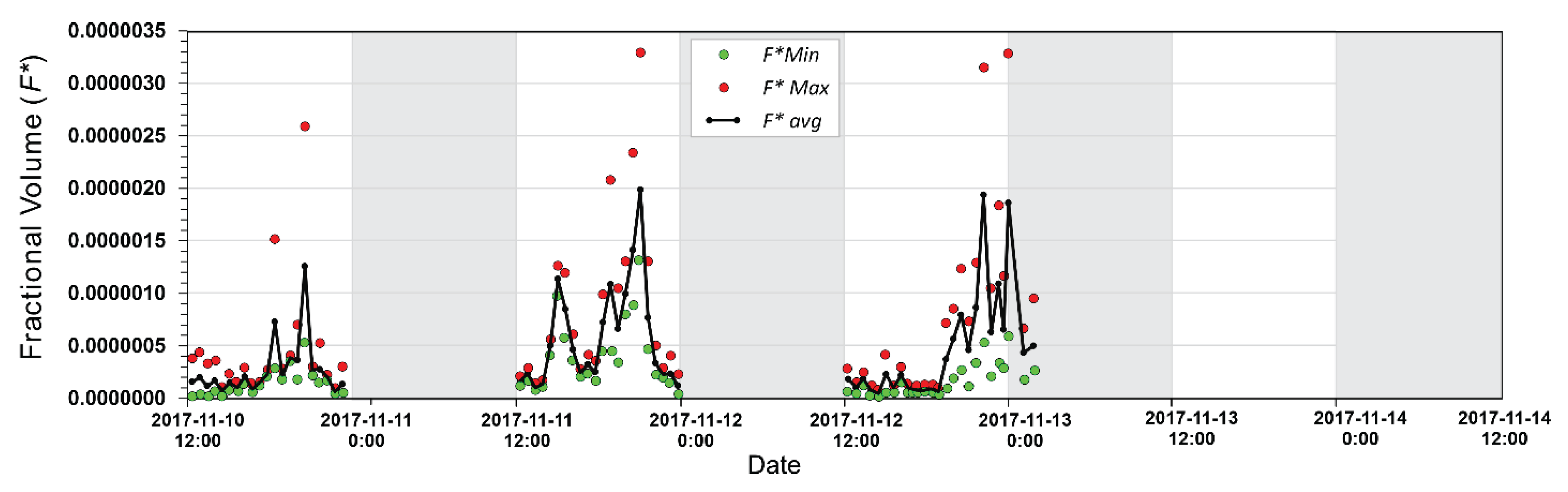
Similar testing of postnoon Frazer et al. (2020) 2-frequency SV data against the alternative elastic sphere algorithm (Faran, 1951) confirmed the feasibility of valid elastic solid ice sphere characterizations for each of the 6 possible acoustic frequency pairs. Fractional volume recalculations were carried out for three different (3,2), (4,2) and (4,3) pairings of 14.2 m SV(t) data constructed from measurements at 200, 455 and 769 kHz after additional 3-point mean filtering. F*(t) values corresponding to averages over all three pairings are plotted at 33 minute intervals along the solid line curve in Figure 3. Additional data markers, denoting maximum and minimum individual pair F*(t) estimates are included to reflect estimate uncertainties. Limitations of manual calculations to three of the six available frequency pairs may have, according to the broken line, 3-frequency, curve in Figure 2a, raised F*avg/F by an additional 10 to 15% for b values above 0.2. With allowances for systematic shape-related underestimates (Marko & Topham, 2015), these results suggest that the F* estimates in Figure 3 are representative of postnoon frazil content variations to within, roughly, a factor of two.
Inspections of initial portions of the recalculated postnoon data plots show the dominance of F*(t) values within a relatively narrow “background” range below 2x10⁻⁷. Data gathered during the first, Nov. 10, daily period, being recorded immediately following instrument de-icing and redeployment, were most likely to be free of icing contamination. The following, Nov. 11, postnoon background stability period was briefly interrupted by an early relative peak in frazil content. All three postnoon periods showed background levels rising sharply at, roughly, 18:00: with F*(t) reaching approximately 2x10⁻⁶ maximum values shortly before precipitous near-midnight descents to low background levels. Overall, the observed patterns of fluctuating, generally increasing, late afternoon and early evening frazil contents closely resembled the typical river frazil variability depicted in Figure 1d but with fractional volumes reduced by as much as 2 orders of magnitude relative to both river values and as represented in Frazer et al.’s (2020) Figure 4e. Such low values and observed negative correlations between river frazil detectability and in situ icing presence justified our initial neglect of icing impacts during, at least, early and middle portions of postnoon intervals.
4.2. Implications for Daily Frazil Production
In assessing the significance of these results, it is useful to note that corresponding Frazer et al. (2020) estimates were interpreted as evidence of “1-9 mm” daily ice accumulations prior to additional in situ growth on sea ice undersurfaces. These estimates were made with references (McFarlane et al., 2014) to frazil rise velocities “up to” 9 mms-1 and, presumably, ignored contributions from unanalyzed prenoon intervals. Although suggested to be compatible with daily 8-10 mm ice accretions inferred from atmospheric heat flux data (Langhorne et al., 2015), the significance of this conclusion is vitiated by unquantified allowances for post-deposition in situ growth on sea ice undersurfaces. Consequently, the quality of frazil production estimates was totally determined by the accuracies of atmospheric heat loss estimates and values of F calculated for postnoon periods with the flawed Kungl et al. (2020) characterization algorithm.
The recalculated postnoon F* estimates in Figure 3 suggested typical daily postnoon frazil production was equivalent to 4 hour presences of 1x10⁻⁶ fractional volumes. Using the 9 mms-1 upper end of the McFarlane et al. (2014) frazil rise rate estimates, such presences corresponded to daily frazil transports to the sea ice undersurface equivalent to a 0.14 mm thick ice layer. Such thicknesses were insignificant relative to both Frazer et al. (2020) estimates and thermodynamic expectations. These results suggest that thermodynamically anticipated levels of MS sea ice accretion could only be attained through in situ growth and/or from prenoon frazil production.
Evidence for the latter possibility is indirect but significant. It draws upon temporal coincidences between prenoon intervals and both icing-driven changes in instrument depth and peaks in supercooled ice shelf water flow toward the measurement site. To be credible, this possibility requires that the low reported prenoon SV values were, as suggested above, consequences of severe acoustic attenuation and multipath scattering endemic to measurements in the presence of in situ icing. Direct insights into these intervals were available, in principle, from effectively zero-range close-in signal returns (Figure 7 in Marko and Topham (2021) and Figure 1d above). Unfortunately, this information was not collected in the Frazer et al. (2020) studies which restricted acoustic data recording to returns from ice targets located at ranges greater than 2 m.
It was useful to make rough estimates of prenoon frazil contents compatible with physical understandings and postnoon F*(t) results. This effort assumed that the mid-postnoon SV(t) increases in Figure 3 persisted into following prenoon intervals. Similar continuity in the Feb.7, 2012 PR echogram (Figure 1d) was evident in early evening strengthening of frazil signal returns which were subsequently extinguished coincidently with the growth of close-in signals which were indicative of attenuations by progressive sensor icing. This behavior supported expectations that observed late postnoon rises in MS frazil contents were more likely to continue than terminate during succeeding prenoon periods which were conspicuously associated with icing-driven instrument destabilizations and lower measured SV values.
Given the impacts of icing on acoustic data collection, it was reasonable to expect that prenoon frazil concentrations considerably exceeded the highest, 2x10⁻⁶, postnoon F* values plotted in Figure 3. This assumption was consistent with the timings of maximal coolings inferred from supercooled ice shelf water flows and peak radiative heat losses through the ice cover. Speculative estimates of corresponding frazil content changes were generated by extending the persistence of typical 0.5x10⁻⁶ h-1 average rates of F*(t) increase during 18:00-22:00 NZST postnoon periods to 06:00 NZST on the following day. This assumption would have raised peak F* values to 6x10⁻⁶ midway through a typical prenoon interval: representing integrated 2.5 mm daily ice contributions to the sea ice undersurface: or about 25% of thermodynamic expectations. Prenoon frazil production in full accord with heat flux losses (Langhorne et al., 2015) would require fractional volumes approaching the 4x10⁻⁵ levels typical of early prenoon river periods (Marko and Topham, 2021).
Definitively quantifying prenoon frazil production requires continuous icing-free access to quantitatively interpretable SV data. In the absence of such capabilities during the Frazer et al. studies, accretion on the 2017 MS sea ice undersurfaces remains an unspecified mixture of in situ growth and water column frazil deposited shortly prior to and during prenoon time periods.
5. Summary and Conclusions
Recent estimates (Frazer et al., (2020)) of frazil production under Antarctic sea ice were undermined by the absence of precautions for avoiding in situ sensor icing. This absence restricted measurements of frazil content to postnoon (12:00-00:00 local time) intervals which, on the basis of variations in atmospheric heat exchanges and influxes of supercooled ice shelf water were associated with minimal frazil growth. This reality was obscured by use of an unvalidated, rheologically incorrect, frazil characterization algorithm.
The present work described and applied a simplified and validated 2-frequency characterization algorithm which identifies absences of convergences in earlier processing procedures and makes credible fractional volume estimates for previously analyzed portions of the daily measurement cycle. Measureable fractional volumes were found to be confined to mid-afternoon to late evening hours, with peak fractional volumes at 14.2 m depths reaching 2x10⁻⁶. Consequent daily contributions to ice cover thickness were less than 0.2 mm: values which were unlikely to be significant relative to ice cover stability issues.
Instrument depth changes indicative of intensive icing during the prenoon (00:00-12:00 local time) intervals excluded from Frazer et al. (2020) characterizations suggest that such intervals were primary hosts of MS frazil production. In the absence of quantitatively interpretable backscattering data from such intervals, speculative extrapolations of postnoon results raised prenoon frazil ice cover growth contributions to, roughly, 25% of thermodynamically-based expectations. It was notable that, in spite of possible differences in crystallization mechanisms, frazil production observed in river studies and measured and tentatively inferred near the McMurdo ice shelf were both primarily confined to early evening through late morning periods centred on times of peak radiative heat losses.
More definitive prenoon frazil estimates require direct access to accurate frazil content data over full daily durations. The technical tools for doing this have been well established in river frazil studies (Marko & Jasek, 2010a,b; Marko et al., 2015; Marko and Topham, 2015, 2021). These studies recognized that: 1) frazil growth in water columns tends to be accompanied by comparable or greater growth on adjacent wet surfaces and; 2) frazil characterization accuracies are highly sensitive to algorithm correspondences with dependences of sound scattering strength on particle dimensions and rheological properties. The 2-frequency methodology allows verifications of such correspondences and, when used with data collected in the absence of significant signal attenuation at 3 or more acoustic frequencies, currently allows convenient estimates of frazil fractional volumes to factor of two accuracies.
MS measurements could supplement externally-heated river measurement methodologies by additionally positioning instruments either below supercooled layers or in downward-looking deployment configurations to suppress needs for and/or facilitate icing clearances. Retention of close-in signal information would also be helpful for interpretative and data quality control purposes. Accumulations of additional acoustic data would support further refinements of theoretical frazil cross section relationships, increasing the accuracies and information content of results obtained from multifrequency characterizations.
References
- Ashton, G.D. (1986). Frazil ice. In: Theory of Multiphase Flow, Academic Press N.Y., 271-289.
- Anderson, V.C. (1950). Sound scattering from a fluid sphere. J. Acoust. Soc., 22, 426-431. [CrossRef]
- Burke, J.E. (1968). Scattering by penetrable spheroids, J. Acoust. Soc., 43, 871–875. [CrossRef]
- Daly, S.F. (1984). Frazil ice dynamics. USACE CRREL Monograph 84-1, Hanover, NH. 86 p.
- Faran, J.J. Jr. (1951). Sound scattering by solid cylinders and spheres. J. Acoust. Soc., 23, 405-418. [CrossRef]
- Frazer, E. K, Langhorne, P.J., Leonard, G.H., Robinson, N.J., & Schumayer, D. (2020). Observations of the size of frazil ice in an ice shelf waterplume. Geophysical Research Letters, 47 e2020/GL090498. [CrossRef]
- Ghobrial. T.R., Loewen, M.R. & Hicks, F.E. (2012). Characterizing suspended frazil ice in rivers using upward looking sonars. Cold Reg. Sci Technol. 86, 113-126. [CrossRef]
- Ghobrial. T.R. & Loewen, M.R. (2021). Continuous in situ measurements of anchor ice formation, growth, and release The Cryosphere, 15, 49–67 . [CrossRef]
- Hay, A. E, and Sheng, J. 1992: Vertical profiles of suspended sand concentrations and size from multifrequency acoustic backscatter. J. Geophys. Res. 97 (10), pp 1566-1567. [CrossRef]
- Hughes, K. G., Langhorne, P. J., Leonard, G. H., & Stevens, C. L. (2014). Extension of an Ice Shelf Water plume model beneath sea ice with application in McMurdo Sound, Antarctica. Journal of Geophysical Research: Oceans, 119, 8662–8687. [CrossRef]
- Kungl, A.F., Schumayer, D., Frazer, E.K., Langhorne,& P.J., Leonard, G.H. (2020). An oblate spheroid model for multi-frequency acoustic back-scattering of frazil ice. Cold Regions Science and Technology 177 (2020)103122. [CrossRef]
- Langhorne,P.J., Hughes, K. G., Gough, A. J., Smith, I. J., Williams, M. J. M., Robinson, N. J., & Haskell, T. G. (2015). Observed platelet ice distributions in Antarctic sea ice: An index for ocean-ice shelf heat flux. Geophysical Research Letters, 42, 5442–5451. [CrossRef]
- Lewis, E. L., & Perkin, R. G. (1985). The winter oceanography of McMurdo Sound, Antarctica. Oceanology of the Antarctic Continental Shelf, 145–165, American Geophysical Union, . [CrossRef]
- Lewis, E. L., & Perkin, R. G. (1986). Ice pumps and their rates. Journal of Geophysical Research, 91(C10), 11756. [CrossRef]
- Marko, J.R. & Jasek, M. (2010a). Sonar detection and measurements of ice in a freezing river I: Methods and data characteristics. Cold Reg. Sci. Technol. 63, 121-134. [CrossRef]
- Marko, J.R. & Jasek, M. (2010b). Sonar detection and measurements of ice in a freezing river II: Observations and results on frazil ice. Cold Reg. Sci. Technol. 63, 135-153. [CrossRef]
- Marko, J. R., Jasek, M., & Topham, D. R. (2015). Multifrequency analyses of 2011–2012 Peace River SWIPS frazil backscattering data. Cold Regions Science and Technology, 110, 102–119. [CrossRef]
- Marko, J. R. & Topham, D.R. (2015). Laboratory measurements of acoustic backscattering from polystyrene pseudo- ice particles as a basis for quantitative frazil characterization. Cold Reg. Sci. Technol. 112, 66-86. [CrossRef]
- Marko, J. R. & Topham, D.R. (2021).Analyses of Peace River shallow water ice profiling sonar data and their implications for the roles played by frazil ice and in situ ice growth in freezing rivers. The Cryosphere, 15, 2473-2489. [CrossRef]
- McFarlane, V., Loewen, M., & Hicks, F. (2014). Laboratory measurements of the rise velocity of frazil ice particles. Cold Regions Science and Technology, 106–107, 120–130. [CrossRef]
- McFarlane, V., Loewen, M. & Hicks, F. (2017). Measurements of the size distributions of frazil ice particles in three Alberta rivers. Cold Reg. Sci. Technol. 142, 100-117. [CrossRef]
- Pietrovich, V.V. (1956). Formation of depth-ice. Translated from Priroda 9: 94-95 by Defense Research Board, D,S.J.S., Department of National Defense, Canada, T235R.
- Robinson, N. J., Leonard, G., Frazer, E., Langhorne, P., Grant, B., Stewart, C., & De Joux, P. (2020): Temperature, salinity and acoustic backscatter observations and tidal model output in McMurdo Sound, Antarctica in 2016 and 2017 - links to original files [Dataset]. PANGAEA, . [CrossRef]
- Smedsrud, L. H., & Jenkins, A. (2004). Frazil ice formation in an ice shelf water plume. Journal of Geophysical Research, 109, C03025. [CrossRef]
- Stanton, T.K, Wiebe, P.H., Chu, D. (1998). Differences between sound scattering by weakly scattering spheres and finite-length cylinders with applications to sound scattering by zooplankton. J. Acoust. Soc. Am. 103 (1). https://doi.org:10.1029/92JC01240.
Figure 1.
Data and additional information relevant to reanalyses. (a) Positions of the 2016 and 2017 MS study sites. (b) Mid-water column PR- and Frazer et al. (2020) 15 m depth-backscattering coefficient, SV, values vs. frequency at indicated times and dates. c) Nov. 10 -14 NZST, 2017 14.2 m SV(t) data plotted for 4 acoustic frequencies with indicated offsets along with changes in instrument depth vs. time during this interval and a preceding Nov. 5-9, 2017 period. The depth change data are plotted referenced to a secondary horizontal time axis shifted forward by 5 days. Background shading and red horizontal lines denote, respectively, prenoon periods and unanalyzed data intervals. d) Echogram display of 774 kHz backscattered signal voltages (in digital counts) vs. range (m) over a 32 h period spanning a Feb. 7, 2012 PR frazil event.
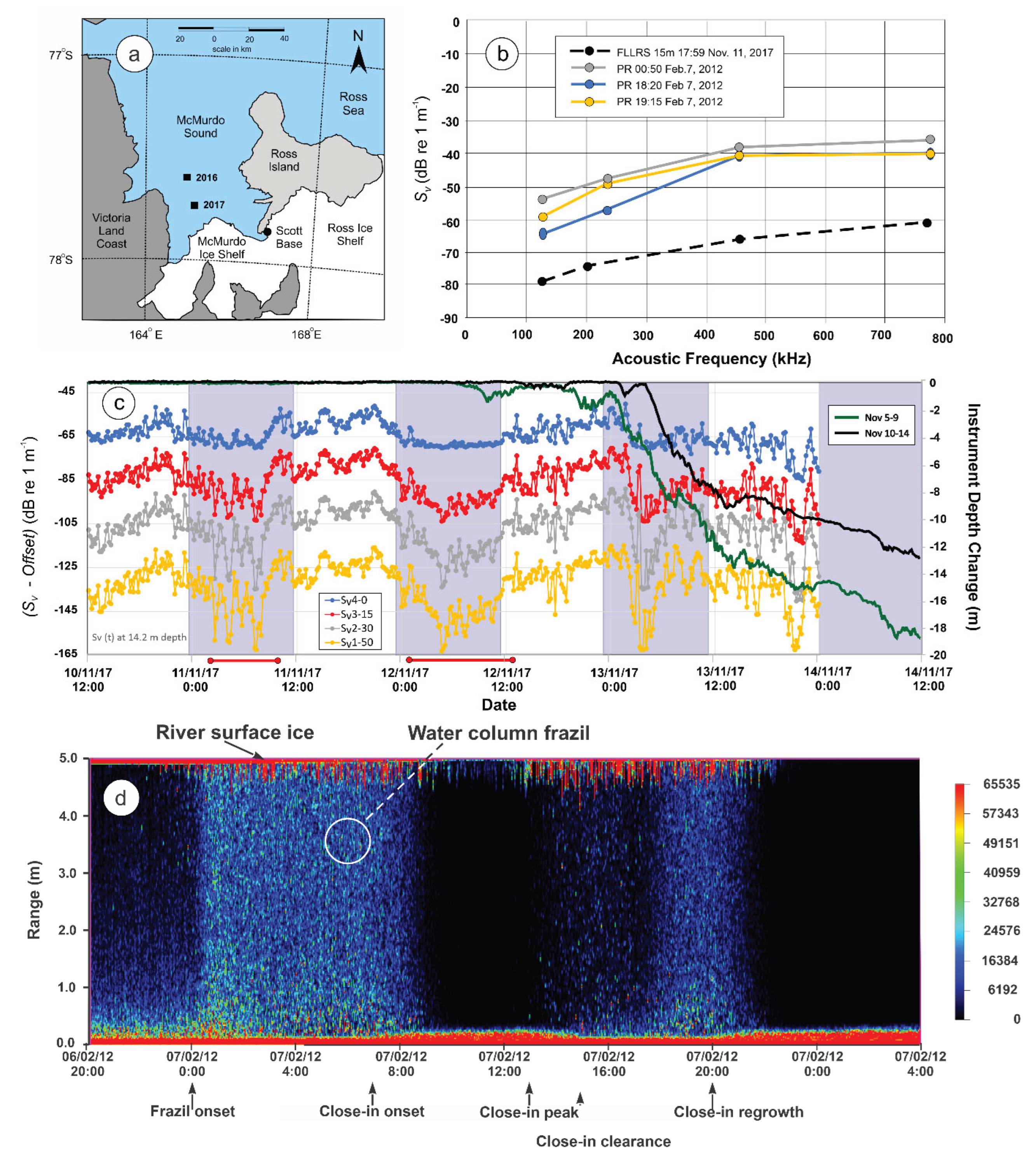
Figure 2.
Results relevant to Kungl et al., (2020) and (Marko et al., 2015) /(Faran, 1951) algorithm comparisons and interpretations of Frazer et al. (2020) data. a) Plots of F*avg/F vs b for an exactly characterized frazil population with F*avg representing 2-frequency average F* estimates using data from 6 and 3 different pairs. b) Normalized backscattering cross sections vs. k1ae for elastic solid and liquid ice spheres in saltwater. A third curve depicts the Kungl et al. (2020) relationship employed in Frazer et al. (2020). c) comparisons of ranges and mean values of pairwise differences in measured cross sections during a 12:06 to 19:59 Nov. 11, 2017 interval with corresponding expectations from elastic solid sphere theory (Faran, 1951) as a function of both effective radius, ae, and disk diameter, D.
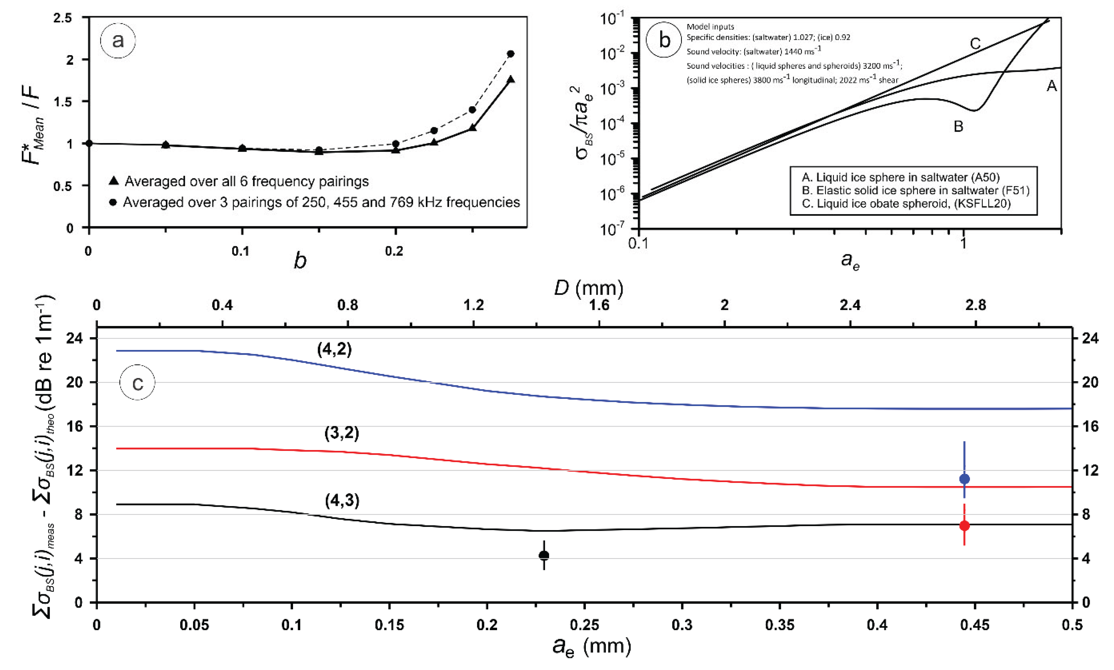
Figure 3.
Plots of means, maxima and minima corresponding to postnoon Nov. 10-13, 2017 2-frequency F* estimates extracted from different, (3, 2), (4, 2) and 4, 3), frequency pairings and an elastic sphere-based algorithm (Faran, 1951).
Figure 3.
Plots of means, maxima and minima corresponding to postnoon Nov. 10-13, 2017 2-frequency F* estimates extracted from different, (3, 2), (4, 2) and 4, 3), frequency pairings and an elastic sphere-based algorithm (Faran, 1951).
Disclaimer/Publisher’s Note: The statements, opinions and data contained in all publications are solely those of the individual author(s) and contributor(s) and not of MDPI and/or the editor(s). MDPI and/or the editor(s) disclaim responsibility for any injury to people or property resulting from any ideas, methods, instructions or products referred to in the content. |
© 2025 by the authors. Licensee MDPI, Basel, Switzerland. This article is an open access article distributed under the terms and conditions of the Creative Commons Attribution (CC BY) license (http://creativecommons.org/licenses/by/4.0/).
Copyright: This open access article is published under a Creative Commons CC BY 4.0 license, which permit the free download, distribution, and reuse, provided that the author and preprint are cited in any reuse.


