
Submitted:
02 December 2024
Posted:
02 December 2024
You are already at the latest version
Abstract
The results of oceanographic observations conducted on board the R/V “Dalnie Zelentsy” along the Kola Section during 2017–2023 are presented. The main focus is on the assessment of frontal zone characteristics in the northern part of the Polar Front during autumn, winter, and spring periods. To estimate sea ice anomalies, data from the World Data Center for Sea Ice (AARI WDC Sea-Ice) were used. A comparison was made between observational data from the northern section near the Marginal Ice Zone and temperature and salinity characteristics from global oceanographic databases. The comparison involved products such as MERCATOR PSY4QV3R1, CMEMS GLORYS12v1, and TOPAZ5. High-gradient zones in temperature and salinity fields were identified along all sections at varying distances from the ice edge. It was confirmed that the western Barents Sea had experienced a steady trend of sea ice cover declining over the past three decades. The northernmost frontal zone of the Polar Front in the Barents Sea, along the Kola Section axis, detected at distances of 48 to 290 km from the ice edge. Temperature gradients ranged from 0.10 to 0.20 °C/km, salinity gradients varied from 0.012 to 0.025 psu/km, and the width of the frontal zone did not exceed 55 km. The best correlation with the measurement results was observed in for the MERCATOR PSY4QV3R1 product.
Keywords:
Temperature
; salinity
; ice conditions
; Polar Front
; marginal ice zone
; Kola Section
; MERCATOR PSY4QV3R1
; CMEMS GLORYS12v1
; TOPAZ5
; Barents Sea
1. Introduction
The Barents Sea is predominantly located in the shelf area and serves as a zone of interaction between Atlantic and Arctic waters (Figure 1). The direction of current flow in the Barents Sea is largely determined by the seabed topography [1,2]. Atlantic waters enter the western part of the sea in two main flows [3]. The primary flow of warm (above 3 °C) and saline (above 34.8 psu) Atlantic waters mainly enters the Barents Sea in the Bear Island Trough with waters from the Nord Cape Current. Additionally, Norwegian and Murmansk coastal currents carry waters with temperatures above 3 °C and salinities below 34.4 psu eastward. These flows to the east are about 2 Sv [4] and 1.1 Sv [5], respectively.
Arctic waters entering from the north and northeast along with drifting sea ice, are formed under the influence of ice melting. As a result, they are characterized by negative temperatures and reduced salinity (below 34.7 psu). Estimating the volume and pathways of these waters remains a subject of debate [2,6], as the presence of sea ice in the northern regions significantly complicates in-situ measurements. Direct current measurements from anchored stations have been conducted at only two locations [2]. Estimates ranging from 0.1 to 0.3 Sv, derived from geostrophic calculations, were later confirmed by model simulations, which indicated a value of 0.36 Sv [2]. In recent decades, the Arctic has experienced more rapid warming than other regions [7]. This warming has been accompanied by observable changes in Arctic Sea ice, including decreases in its area and thickness, resulting in a significant declining in ice volume [8,9]. These changes also influence the volume of Arctic waters entering the Barents Sea.
An important consequence of the interaction between Atlantic and Arctic waters in the Barents Sea is the presence of the North Polar Frontal Zone [10] or the more commonly used term Polar Front (PF) [11,12]. This zone is characterized by pronounced horizontal and vertical gradients of thermohaline properties, spanning spatial scales of several tens of kilometers. The frontal zone in the Barents Sea region is considered quasi-stationary, with its position associated with the slopes of major elevations, including the Spitsbergen Bank, Central Bank, and Perseus Bank. Typically, the frontal zone is observed near the 200-250 m isobath [3,11]. However, [4] demonstrated that climate changes in the Barents Sea affect the position of the front south of Bear Island. During warmer periods with stronger winds, the front shifts upward along the slope compared to colder periods. It is evident that in the Central Bank area, where the PF is less stationary in nature [3], the fluctuations may be even more pronounced.
One of the key factors determining the hydrological regime of the Barents Sea and reflecting its variability is the presence of sea ice cover [13]. The ice cover influences the interaction between the ocean surface and the atmosphere, affecting the sea's heat balance and the interaction between waters of different origins, especially in the active layer of the ocean. The mean boundary of ice distribution in the Barents Sea lies to the north of the PF [14] and is known as the Marginal Ice Zone (MIZ). The MIZ is defined as a transitional area between the open ocean and dense drifting ice. It extends from an arbitrary line where 15% of the sea surface is ice-covered to the position of the 80% ice concentration isoline [15]. Notably that near the Marginal Ice Zone, a distinct haline frontal zone is typically observed during the warm season. Its existence is caused by the influx of a large volume of meltwater. The influence of this meltwater can be detected several tens of kilometers away from the ice edge [16].
In the context of climate change, there is a noticeable acceleration of warming rates in the Arctic, known as "Arctic amplification" [17,18,19,20,21,22,23]. Against this backdrop, the Barents Sea has seen the most significant declining in sea ice cover among Arctic seas [24], coupled with an overall increase in the average temperature of the air–ice–ocean system [25]. As a result, the Barents Sea becomes the first ice-free sea in the Arctic Ocean during the summer period. However, in the autumn, winter, and spring, sea ice forms in the northern part of the sea. As sea ice extent decreases, the intensity of interactions within the ocean–atmosphere system increases. Consequently, current climate conditions differ from those of previous years due to the increased air temperature across all seasons [2], inevitably affecting the position and characteristics of frontal zones in the sea. The first decades of the 21st century have been marked by a declining in the area of sea ice in the Barents Sea, positive temperature anomalies of sea surface temperature and near-surface air temperature, and an increase in the temperature of intermediate and deep waters [21,26,27,28]. According to [29], the average annual heat balance at the surface of the Barents Sea between 1993 and 2018 was negative throughout the entire sea. Winter heat flux from the sea surface has increased during the cold season, raising the average annual heat balance at the sea surface due to reduced ice cover and higher temperatures of Atlantic-origin waters entering from the Norwegian Sea. Studies [30,31,32] have shown that interannual variations in sea ice extent in the Barents Sea exhibit a significant negative linear trend, similar to that of the entire Arctic region. The average annual ice cover of the Barents Sea has declined by 14.6% per decade in recent decades [23].
Hydrological fronts that occur at the boundary between Atlantic and Arctic waters are an important oceanographic feature of the Barents Sea. However, due to inaccessibility, they were insufficiently studied during the cold season [16]. Currently, research is being conducted intensively [3,11,12,33,34], and we aim to expand the description of the northern part of the polar front through unique recurring measurements conducted in the northern part of the Kola Section. The transect follows the meridian 33°30’ E [35], and measurements have been conducted there for more than a century (the first works were carried out in May 1900). Over the past century, numerous studies have been conducted [1,36,37,38,39,40,41]. Observations along this transect allow for monitoring seasonal and interannual changes in oceanographic parameters along the path of Atlantic-origin waters, which also influence the characteristics of the Polar Front. However, in many of cases, works on this transect were not conducted north of 74°N during the ice formation period. Only in recent decades, during the active declining of sea ice extent in the Barents Sea, have studies by Murmansk Marine Biological Institute of the Russian Academy of Sciences (MMBI RAS) along the transect been regularly conducted up to the MIZ [42].
Studies along the Kola Section aim to continuously monitor the marine environment, enhancing the quality of forecasts for anticipated changes. At the current stage of research, addressing this task involves developing numerical models that incorporate operational assimilation of satellite, drifter, and ship-based observational data. Global ocean reanalysis systems are continually evolving, and their outputs are publicly accessible (e.g., Copernicus Marine Environment Monitoring Service, Arctic Ocean Physics Analysis and Forecast). The generated spatio-temporal fields of oceanographic characteristics are regularly updated and allow for the reproduction of oceanic fields of temperature and salinity, which are considered verified. However, regular data from Arctic seas are only available from certain satellite observational systems and coastal stations. Irregular data, obtained from local areas of the sea during marine expeditions, often do not enter the assimilation models due to fragmentation and stringent internal regulations of marine organizations and research institutes. Independent verification of the products is rarely conducted, i.e., involving databases not involved in the development of the analyzed models. The availability of a unique data set allows for the assessment of the quality of oceanographic field reproduction by different types of reanalysis.
The aim of the study is to assess the variability of Polar Front characteristics in the northwestern Barents Sea based on in situ observations along a regularly conducted hydrological transect, accounting for changes in sea ice extent. Additionally, the study aims to evaluate the quality of oceanographic field reproduction using various reanalysis and forecasting products.
2. Materials and Methods
This study uses expedition data collected by MMBI RAS in the western Barents Sea [43,44] on board the research vessel “Dalnie Zelentsy” from 2017 to 2023. Oceanographic research was conducted along the "Kolski Meridian" transect (Figure 1). Key hydrological parameters of the marine environment were measured using CTD casts with a SEACAT SBE 19 Plus V2 profiler. This work includes a series of oceanographic measurements taken from 69°30' N along the 33°30' E meridian to the ice edge, with a spacing of 15-30 nautical miles across different seasons from 2017 to 2023 (Table 1). Due to the technical specifications of the “Dalnie Zelentsy” research vessel, measurements were conducted in conditions of low ice consolidation (1-3 points on the ice scale).
For the verification and supplementation of visual observations of the ice edge conducted from the R/V, data from the U.S. NATIONAL ICE CENTER archive were used (U.S. National Ice Center: [website]; URL: https://usicecenter.gov/Products/ArcticHome, accessed on 20.09.2024). These data represent a Shapefile containing vector information on the location of the Marginal Ice Zone, where sea ice concentration is less than 80%, and the pack ice zone, where the ice concentration is greater than 80%.
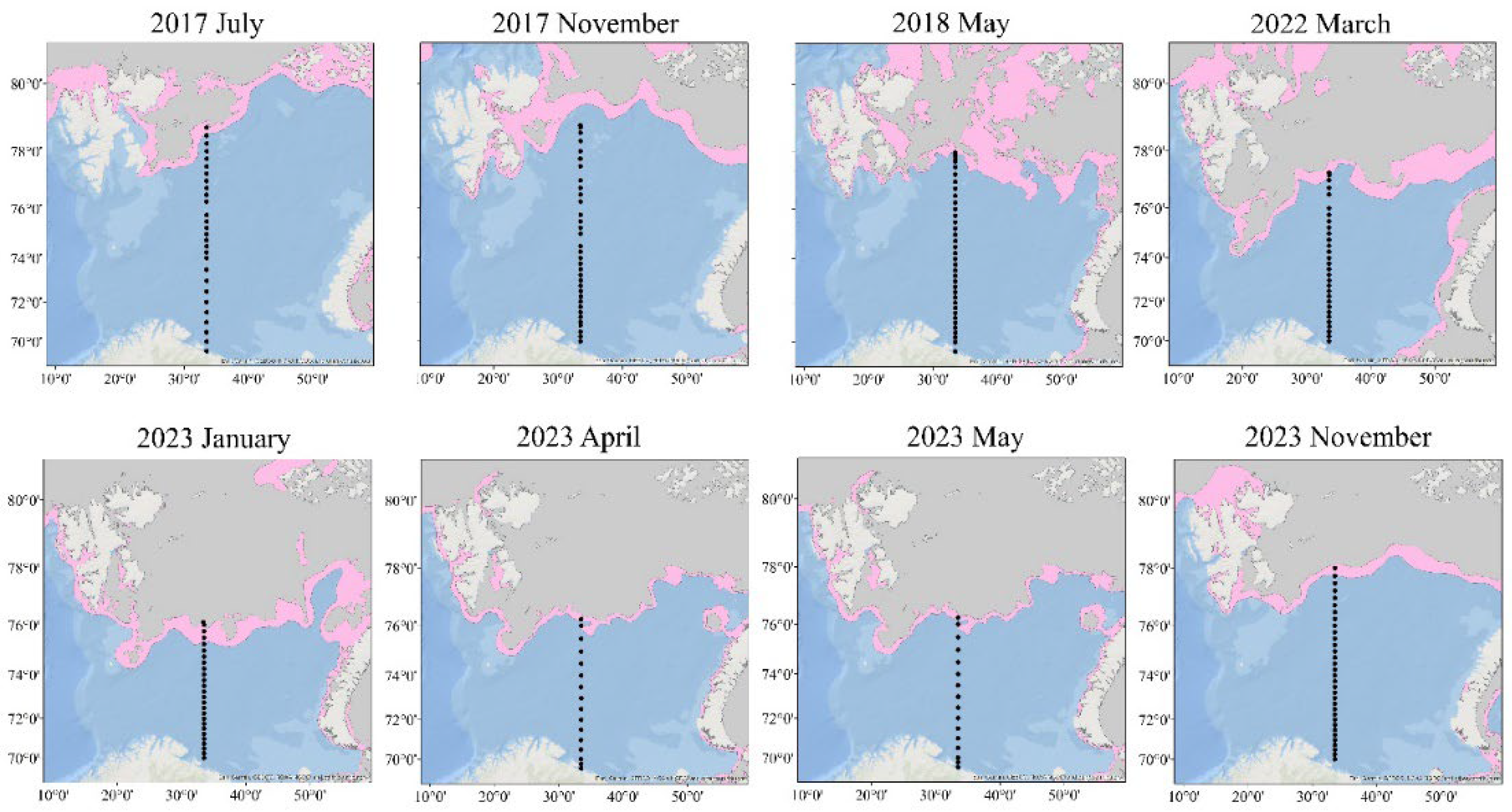
Figure 2.
Location of the oceanographic stations along the Kola Section on the map of the Barents Sea. The position of the MIZ is highlighted in pink (1-8/10 concentration), and areas of consolidated ice (> 8/10 concentration) are shown in gray.
Figure 2.
Location of the oceanographic stations along the Kola Section on the map of the Barents Sea. The position of the MIZ is highlighted in pink (1-8/10 concentration), and areas of consolidated ice (> 8/10 concentration) are shown in gray.
The main source of ice information was the Arctic and Antarctic Research Institute's (AARI) ice charts, compiled by ice experts with many years of experience. The archive of ice charts is collected in the electronic catalog of the World Data Center for Marine Ice (AARI WDC Sea_Ice: [website]. URL: http://wdc.aari.ru/datasets/d0015/ (accessed on 28.09.2024)). In the construction of ice charts, satellite images in various electromagnetic spectrum ranges (visible, infrared, and microwave) are used to obtain the necessary information about the ice cover, supplemented by data from ship-based observations and polar hydrometeorological stations. The AARI ice charts are available with weekly frequency, starting from October 1997 to the present. A detailed description of the methodology for compiling AARI ice charts is presented in the paper by Afanasyeva [45]. As a result, ice cover was calculated as a percentage of the area of the western region, which is one of the homogeneous ice-hydrological zones of the Barents Sea, within the commonly accepted boundaries. The lower limit for the determination of ice concentration is 10% (corresponding to 1 point on the ice chart).
The classification of monthly ice conditions anomalies was performed according to the methodology in [46]. The average monthly ice anomalies (ΔS_ice) were compared with the given values of the standard deviation of ice concentration from the 27-year average, σ. The average monthly ice anomalies, calculated for the western region of the Barents Sea, were classified into five categories (Table 1).
The criterion for evaluating the thermal state of the waters in the Barents Sea was the ratio of water temperature anomalies (ΔT) in the 0–50 m layer at standard stations along the Kola Section profile (69°30′ — 74° N, with a 30′ interval) for each period (month) when contact measurements were made, and the standard deviation of water temperature (σ) categorized into five gradations [47,48] (Table 2). For calculating the anomalies, monthly water temperature norms were used, derived from data from 1970 to 2019 from the World Ocean Database (NOAA World Ocean Database: [website]. URL: https://www.ncei.noaa.gov/products/world-ocean-database (accessed: 1.09.2024), ICES (ICES: [website]. URL: https://www.ices.dk/data/data-portals/Pages/ocean.aspx (accessed: 1.09.2024), and local databases from the MMBI RAS. The norms and anomalies were calculated with a five-meter depth interval.
The frontal zone is an area within which spatial gradients of temperature and salinity (Grad_T and Grad_S) are significantly sharper compared to climatological values [49]. Therefore, the gradients in the frontal zone must substantially exceed the average climatological gradient (Grad_Climat). In [49], it is suggested to identify frontal zones when Grad_T, S > 10 Grad_Climat. Climatological values for the horizontal temperature and salinity gradients for the Barents Sea, according to [10], do not exceed 0.01 °C/km and 0.001 psu/km, respectively. The width of the frontal zone was determined as the distance between points (stations) along the profile, beyond which the temperature and salinity gradients approach climatological values. Isotherm 1.5 °C and isohaline 34.7 psu, characteristic of the position of the main frontal boundary (the line corresponding to the maximum gradient values within the frontal zone), were selected between such stations.
To assess the impact of wind forcing on the dynamics of the ice edge position, the U and V components of the hourly wind speeds at 10 m height from the ERA5 reanalysis were used (ECMWF: [website]. URL: https://cds.climate.copernicus.eu/datasets, accessed: 1.11.2024). The wind speed and direction in knots were calculated at the grid points corresponding to the first point north of the ice edge position along the meridian 33°30’. Additionally, air temperature at 2 m height was taken from the reanalysis, averaging over the segment of the profile from the position of the frontal zone to the ice edge. The period considered was four days: three days prior to the ice edge measurements and the day of the measurements.
To compare the results of CTD profiling with operational ocean model data, daily data from the following products were used:
- —
- MERCATOR PSY4QV3R1 (Global ocean 1/12° physics analysis and forecast updated daily: [website]. URL: https://data.marine.copernicus.eu/product/GLOBAL_ANALYSISFORECAST_PHY_001_024, accessed: 05.09.2024);
- —
- TOPAZ5 (Arctic Ocean Physics Analysis and Forecast: [website]. URL: https://data.marine.copernicus.eu/product/ARCTIC_ANALYSISFORECAST_PHY_002_001, accessed: 05.09.2024);
- —
- CMEMS GLORYS12v1 (Global ocean physics reanalysis: [website]. URL: https://data.marine.copernicus.eu/product/GLOBAL_MULTIYEAR_PHY_001_030, accessed: 05.09.2024).
The selection of the CMEMS GLORYS12v1, MERCATOR PSY4QV3R1, and TOPAZ5 products was based on their high spatial and temporal resolution for the study area. The CMEMS GLORYS12v1 product from the Copernicus Marine Environment Monitoring Service is a global ocean reanalysis with daily resolution and a spatial resolution of 1/12°. The MERCATOR PSY4QV3R1 product, the operational global ocean analysis and forecasting system of the European group, has the same resolution. The TOPAZ5 daily data set, which uses the HYCOM model, provides information for the Arctic region with a spatial resolution of 6.25 km for the output data.
The area from 74° to 80° N and 33° to 34° E was extracted from the products, containing data on the distribution of temperature and salinity in the 0–50 m layer across 19 depth levels corresponding to the grid nodes of the CMEMS GLORYS12v1 and MERCATOR PSY4QV3R1 products, and 11 depth levels for the TOPAZ5 product. For the comparative analysis, uniform arrays were formed by aligning measurement data and model products to common coordinates, depth levels, and dates of each station along the transect. All data along the transect were interpolated using the Kriging method [50], which provides the best linear unbiased estimate of field characteristics on a regular grid, in Surfer software. The comparative analysis included both qualitative and quantitative assessments of how well the reanalysis and forecast data corresponded to the in-situ measurements.
For the comparative analysis, the Modified Hausdorff Distance (MHD) was used. This metric is often employed for quantitatively assessing the similarity between the spatial distribution of modeled and observed scalar fields of various hydrometeorological parameters [51,52]. In the frontal zone, the isotherm of 1.5 °C and the isohaline of 34.7 psu, corresponding to the center of the frontal zone based on in-situ data, were selected. For the selected products, the same isotherms (temperature) and isohalines (salinity) were chosen. Each point on the isotherm had its own coordinates, with the x-axis representing the distance along the transect in kilometers and the y-axis representing the depth. As a result, Set A formed a set of points (with coordinates along the x and y axes) based on in-situ observations, and Set B formed a set of points from one of the products. Further explanations are given in terms of set theory. For the comparison, the characteristic isotherm of 1.5 °C and isohaline of 34.7 psu, typical for the position of the maximum gradient in the frontal zone, were selected.
Initially, the minimum distance from the set of points A to each point b was calculated (1), followed by a similar calculation from each point a to the set of points B (2).
Next, the average minimum distances within the sets are calculated (3).
where |A| and |B| are the number of points in each set, respectively. At the final stage, the maximum value is selected from the available average minimum distances between the sets of isoline points (4) for each horizon.
For a qualitative assessment in the frontal zone between two stations where the FZ was located, the gradient at each depth was calculated based on the data (in the case of in situ data interpolated to depths for CMEMS GLORYS/MERCATOR PSY4QV3R1 and TOPAZ5). The weighted average gradient was then computed. The difference (An. Grad) between the weighted average gradient based on in situ data and the weighted average gradient of the product was assessed. The significance of the difference was evaluated using the Student's t-test [53], which was compared with the critical value. If the calculated value was greater/less than the critical value, the differences between the weighted averages (An) were considered significant/insignificant, respectively.
3. Results
3.1. Changes in Ice Cover in the Western Barents Sea
According to the annual average data, the ice cover in the western Barents Sea has been decreasing over the past 30 years (Figure 3). Maximum ice coverage during the observed period occurred in 2003, while minimum coverage was recorded in 2016. Since 2018, a steady declining in the ice-covered area has been observed. Over the past decade, the ice area has decreased by 4.4%, which is approximately three times less than the declining observed across the entire sea [23]. In addition to the pronounced negative trend in ice coverage in the western region, interannual variability also contains cyclic components with periods ranging from 4 to 11 years, which significantly contribute to the variability of the series. In the study [23], a larger dataset (from 1979 to 2022) of ice coverage values in the Barents Sea revealed cycles with periods of 4, 5.5–11, and 22 years, corresponding to cycles of global meteorological indices (Arctic index, North Atlantic Oscillation, etc.), the 11-year solar activity cycle (Schwabe-Wolf cycle), and the Hale solar cycle (22 years).
Monthly anomalies of ice coverage in the studied region for the periods of work along the Kola Section (Table 1) are shown in Table 3. These anomalies indicate the absence of positive ice coverage anomalies during any the months of the expeditionary studies. Negative anomalies were observed twice in May, suggesting an earlier onset of the ice melting process in recent years. In contrast, water temperature anomalies in the 0–50 m layer along the Kola Section exhibited normal and positive values.
The results confirm that the variability of the ice regime in the Barents Sea is uneven, with most of this variability occurring in the central and northeastern parts of the sea [54]. The maintenance of the ice-free southwest Barents Sea is significantly influenced by the influx of Atlantic-origin waters, as shown in studies [55,56].
Hydrological and ice conditions related to the intensity of Atlantic water inflow were analyzed during in situ measurement periods along the Kola Section (Table 1). An assessment of water temperature anomalies in the 0–50 m layer at section stations and ice concentration anomalies in the western Barents Sea revealed a strong correlation between the two (Table 2). Positive water temperature anomalies corresponded to negative ice concentration anomalies in the western Barents Sea. Close to average/norm conditions, temperature anomalies were observed in July 2017 and November 2022. Other observations along the section were conducted under conditions of significant positive water temperature anomalies and normal to strongly negative ice concentration anomalies.

Table 3.
Classification by type of anomaly.
| Measurement period | Type of average monthly ice coverage anomaly | Type of temperature yufenanomaly |
|---|---|---|
| 2017 July | N | N |
| 2017 November | -SA | +VSA |
| 2018 May | -SA | +VSA |
| 2022 March | N | +SA |
| 2023 January | -SA | +VSA |
| 2023 April | N | +SA |
| 2023 May | -SA | +SA |
| 2023 November | N | N |
(Type of anomaly: Very strong positive anomaly (+VSA), Strong positive anomaly (+SA), Close to average/norm (N), Strong negative anomaly (-SA)).
During the months analyzed in the last decade, predominantly anomalously warm years and warm conditions in terms of water temperature were observed, corresponding to significant negative and normal ice coverage anomalies in the western Barents Sea. This reflects the ongoing trend of significant ice cover declining in the Barents Sea over recent decades. The effects of these changes on the characteristics of the frontal zone will be examined in the following section.
3.2. Characteristics of Water Along the Kola Section During the Summer Season
Water temperature and ice coverage anomalies were close to normal in July 2017 (Table 3). Therefore, we will analyze the structure of the water along the section based on observations from July 13–17, 2017 (Figure 5), to evaluate water characteristics during a period without significant extremes in the Barents Sea. The ice melting season in the Barents Sea begins in May and lasts until September, during which the ice edge retreats northward and eastward [2]. Stations along the Kola Section can be grouped into five categories based on the currents crossing the section (Figure 1). The positions of boundaries between station groups may vary depending on climatic conditions and the impact of synoptic-scale processes.
The first group of stations is located in the waters of the Murmansk Coastal Current (69°30'–70°00' N). Here, the freshwater influence from river runoff is observed, which results in a pronounced halocline throughout the year. In July 2017, this halocline was observed in the 0–10 m layer, with a salinity gradient of 1.6 psu and a temperature gradient of 4.9°C. The average temperature and salinity at the stations were 5°C and 34.4 psu.
The second group of stations is crossed by the Murmansk Current (70°30'–71°30' N). In this section of the transect, the Murmansk Coastal Current interacts with the Murmansk Current. The influence of river runoff gradually decreases toward the north, and the halocline rises to the surface. The average temperature and salinity in this area in July 2017 were 5°C and 34.7 psu. At the northern boundary of this station group, the Coastal Front Zone is observed, manifested in the salinity field.
The third group of stations belongs to the Central Branch of the North Cape Current (72°00'–74°00' N). This group of stations has the most homogeneous structure during the winter period, both in terms of temperature and salinity. In summer, a warm upper layer and colder bottom waters are observed. The average temperature and salinity values were 4.1°C and 35 psu.
The fourth group is in the area of influence of the Northern Branch of the North Cape Current and the Central Current (74°15'–76°15' N). The upper 50-meter layer is occupied by warm Atlantic waters, with average temperature and salinity values of 4.2°C and 34.9 psu. Below the Atlantic waters, a dome of cold, salty Barents Sea waters is observed, with average temperature and salinity values of 2°C and 35 psu. The northern part of this area contains the Polar Front of the Barents Sea.
The fifth group of stations is located in the area influenced by the Perseus Current (76°30'–80°00' N). Here, cold Arctic waters with temperatures below 0 °C are observed. Freshened waters, formed as a result of mixing local waters with meltwaters, occupy a layer from the surface to 100 meters. The average temperature and salinity in this layer were -0.1°C (excluding the warmed upper 20-meter layer) and 34.5 psu. The minimum temperature was -1.8°C. The most freshened layer, from the surface to 15 meters, characteristic of the active ice-melting period, was observed in the northern part of the section, with the minimum salinity of this layer being 32.2 psu.
At the boundary between the fourth and fifth groups of stations, there is the Polar Front of the Barents Sea, located in the area of the Perseus Current slope. This frontal zone is often situated close to the ice edge or is entirely covered by ice of varying cohesion during the winter period. The existence of the frontal zone is due to the interaction between the Arctic waters of the Perseus Current and the Atlantic waters of the Northern Branch of the North Cape Current. Since the Polar Front is an area where cold, fresh waters from the Arctic basin interact with warm, salty Atlantic waters, it is expressed both in the temperature field and the salinity field. The zones of sharp gradients in temperature and salinity do not always coincide, and in the salinity field, a double (stepped) structure is observed. This frontal zone has a quasi-stationary nature and exists throughout the year.
Measurements in the Polar Front area were taken from July 15 to 17, 2017. During this time, the average air temperature at a height of 2 meters (according to Era5 data) was 3.14°C, with a prevailing southward wind at a speed of 5.2 m/s. The ice edge was observed at 78°35′ N. The upper 20–25-meter layer was warmed to 2°C. The area of maximum vertical temperature gradients extended under the warmed waters up to 150 meters. The width of the frontal zone was about 55 km, with a temperature gradient of 3.1°C at a 30-meter depth. North of 78°30′ N, Arctic waters had a negative temperature from the surface to the bottom and were within the Polar Front Zone (PFZ). The maximum horizontal temperature gradient was -12 Grad_Climat, and the salinity gradient was 14 Grad_Climat. Two areas of increased salinity gradients were distinguished along the section. The first area was observed near the slope of the Perseus Bank, where the Polar Front Zone is located. The second area of increased gradient was found 65 km from the ice edge, where it was more pronounced in the salinity distribution. Here, a 0–10-meter layer of the most freshened and coldest waters, formed directly by ice melt in the study area, was observed, with the minimum salinity of 32.1 psu. It is also worth noting that this distribution [10] is called “stepwise,” distinguishing types of internal structure in frontal zones along with “interspersed” ones. In this section of the Polar Front, such a “stepped” type is characteristic only in the summer season in the salinity distribution when active ice melting occurs. Thus, the first zone corresponds to the Polar Front of the Barents Sea, while the second freshened zone corresponds to the Arctic Frontal Zone [10], whose formation is associated with ice melting in the warm period of the year. This last frontal zone is often noted in the PF area, as it was in this case (see Figure 2a).
3.3. Characteristics of Waters Along the Kola Section During the Ice Formation Period
The remaining measurements were primarily taken during the winter season, when Sea ice formation period in the Barents Sea typically begins. The sea ice formation period in the Barents Sea typically begins in early October in the northern regions and lasts until March-April, when the ice cover reaches its maximum extent [2]. The studies conducted in November 2017, January 2023, and November 2023 mark the beginning of the ice formation period. During this time, the waters are relatively homogeneous, unaffected by radiation heating and additional freshening due to ice melt.
At the end of November 2017 and January 2023, measurements were taken under conditions of a very large positive anomaly in water temperature in the 0–50 m layer and a large negative anomaly in ice cover in the western Barents Sea. As a result, the waters were warmer than usual, and the area covered by ice was smaller than in "normal" conditions. In the "normal" ice-cover and water temperature anomaly conditions for the western Barents Sea, measurements were taken in November 2023. During the periods of measurement, air temperatures were below freezing, the prevailing wind direction varied from year to year, and the average wind speed did not exceed 6.3 m/s. The southern boundary of the thermal frontal zone varied from 76°15′ in November 2017 and January 2023 to 76°30′ in November 2023. The width of the frontal zone was about 30 km, and vertically, the boundary of the thermal frontal zone extended from the surface to 100-150 m. Since, at the beginning of the winter period, the ice cover forms from the northern part of the sea towards the south, the frontal zone was located at a considerable distance from the ice edge. For example, in November 2017, the thermal and haline frontal zones were almost 300 km from the ice edge. The maximum horizontal temperature gradient at the beginning of the ice formation period exceeded the climatic norm by 10 to 16 times, and the maximum salinity gradient was 13 to 25 times greater than normal.
Table 3.
Position and characteristics of the Polar Front along the Kola Section.
| Measurement period | The position of the thermal frontal zone, N | Maximum temperature gradient, °C/km | Position of the salinity frontal zone, N | Maximum salinity gradient, psu/km |
|---|---|---|---|---|
| 2017 July | 76°00' - 76°30' | 0.12 | 75°45' - 76°00' | 0.014 |
| 2017 November | 76°30' - 76°45' | 0.11 | 75°15' - 76°45' | 0.025 |
| 2018 May | 76°00' - 76°30' | 0.12 | 76°00' - 76°30' | 0.021 |
| 2022 March | 76°00' - 76°30' | 0.12 | 76°00' - 76°30' | 0.025 |
| 2023 January | 76°15' - 76°30' | 0.16 | 76°15' - 76°45' | 0.020 |
| 2023 April | 75°30' - 75°45' | 0.10 | 75°30' - 76°00' | 0.012 |
| 2023 May | 76°00' - 76°15' | 0.20 | 76°00' - 76°15' | 0.018 |
| 2023 November | 76°30' - 76°45' | 0.10 | 76°30' - 76°45' | 0.013 |
At the end of the ice formation season, when the ice cover in the Barents Sea reaches its maximum extent, measurements were taken in May 2018, March 2022, April, and May 2023. All measurements during this period were taken under conditions of a very strong (May 2018) and strong positive anomaly (March 2022, April, and May 2023) in temperature along the section and normal (March 2022 and April 2023) and strong negative anomaly (May 2018 and 2023) in ice cover in the western Barents Sea. The prevailing wind in March 2022 and April 2023 was from the north, with average speeds of 11.7 and 10.7 m/s, while in May 2018, the prevailing wind was from the east (4.6 m/s), and in May 2023, from the south (4.8 m/s). During the study period, the thermal and haline frontal zones coincided along the section. Compared to the start of the winter period, the frontal zone shifted south by 110 km in April 2023 and by 55 km in the other periods. The width of the frontal zone ranged from 30 to 55 km. The frontal zone was closest to the ice edge in April 2023 (see Figure 6b). During the measurement period, three northern stations along the section were within the marginal ice zone. The frontal zone shifted south to 75°30′ N. The southward shift of the frontal zone was likely caused by the impact of the northern wind, which had a relatively high average speed (10.7 m/s). Two weeks later, measurements were taken again along the section. The frontal zone had shifted north to 76°00′ N, with the prevailing southern wind pushing the ice with Arctic waters to the north.
The boundary of the thermal frontal zone shifts southward during the spring months. Thus, at the beginning of the ice formation period (January and November, Figs. 6, ab, gh), the thermal component of the Polar Front was located above the slope of the Persey Bank, while at the end of this period (April, May, Figs. 6 cd, ef), it was observed above the Central Bank. The frontal zone was closest to the ice edge (48 – 72 km) at the end of the ice formation period (April and May 2023), which was associated with the southward displacement of Arctic waters along with the ice cover. The haline frontal zone exhibited greater variability than the thermal one. At the end of the ice formation period, a more complex temperature distribution structure was observed in the area of the Polar Front compared to the earlier months of the season. An "alternating" temperature distribution was seen, characterized by the alternation of cold and warm patches of varying widths, separated by local fronts. The formation of such a structure could have been caused by both advection processes and the influence of vortices, which frequently form in the frontal zone [10].
3.4. Assessment of the Reproducibility of Water Characteristics in the Northwestern Barents Sea
To assess the quality of the reproduction of thermohaline fields in the area of the Polar Front of the Barents Sea along the Kola Section, a comparison was made between CTD profiling data and simulation results. Three measurement datasets were considered, collected during the sea ice formation period (January and November 2023) and during the transition from ice formation to ice melt (April 2023). The characteristic isolines for maximum temperature and salinity gradients (1.5 °C and 34.7 psu) were compared between in situ data and reanalysis data. In general, for all the considered months, the isotherm was located almost perpendicularly downward (Figure 7 a-c). The in situ isotherm was closest to the CMEMS GLORYS12v1 in April (1.1 km) and the MERCATOR PSY4QV3R1 in January (2.6 km). In other cases, the isotherms were located more than 3 km apart according to the MHD. The best result (minimal distance) for the 34.7 psu isohaline was shown by TOPAZ5 in January, with an MHD value of 5.3 km. However, in November of the same year, this value was nearly 14 times greater. The isolines for all products did not completely match with the in situ isolines, which is confirmed by the values presented in Table 4.
Table 4 also presents the values of the difference (An. Grad) between the weighted averages of the gradients inside the frontal zone based on in situ data and the products MERCATOR PSY4QV3R1, CMEMS GLORYS12v1, and TOPAZ5. In general, the differences in the mean values, according to the Student's t-test, were significant with all products in all months, except for the values of the MERCATOR PSY4QV3R1 product for salinity in January, where the difference between the weighted averages was insignificant and nearly 0°C/km. For temperature, the difference ranged from 0.026 to 0.072°C/km and was significant, while for salinity, the gradient differences were almost always significant, ranging from -0.0007 to 0.0101 psu. This indicates that while the selected products qualitatively do not reflect the actual gradient values within the frontal zone, they provide a sufficiently accurate depiction of the position of the frontal zone for assessing its dynamic behavior on different temporal and spatial scales. When comparing the reanalysis results integrally across the three months under consideration, the MERCATOR PSY4QV3R1 product was identified as the best for representing real conditions. The MHD for the 1.5°C isoline had values up to 10.3 km, and for the 34.7 psu isohaline – 26.2 km, with the maximum distance between isolines (69.2 km) observed for the TOPAZ5 data.
The analysis of qualitative and quantitative evaluations from the comparative analysis showed that reanalysis and forecast products do not reproduce the actual values of temperature and salinity within the frontal zone in January, April, and November 2023. However, the reanalysis data do not guarantee obtaining the real values of temperature and salinity in the Barents Sea. At the same time, they adequately describe the patterns of distribution of the studied parameters. This study demonstrated that the global product MERCATOR PSY4QV3R1 provided the closest values of the gradient and the position of isolines characteristic of the frontal boundary during the freezing period (January and November 2023). In the transitional period, when the sea experiences maximum coverage in the annual cycle and the melting process begins (April 2023), the variability of temperature and salinity in the Polar Front was well reproduced by the regional reanalysis product TOPAZ5.
4. Conclusions
The study presents the results of oceanographic observations conducted on board the R/V “Dalnie Zelentsy”, primarily in the northern part of the Kola Section over various seasons from 2017 to 2023. The position and characteristics of the Polar Front in the Barents Sea along the Kola Section are discussed during periods of active sea ice formation, maximum ice cover, transition to ice melt, and in the summer period when the ice edge is at its northernmost position. The study mainly focuses on the dynamic upper layer of 0–50 meters, which is more susceptible to variability due to the ocean-ice-atmosphere system. It is shown that the northernmost section of the Polar Front along the Kola Section is located at distances ranging from 48 km to 290 km from the ice edge. Temperature gradients varied from 0.10 to 0.20 °C/km, and salinity gradients ranged from 0.012 to 0.025 psu/km, with the width of the frontal zone not exceeding 55 km. The position of this frontal zone is quasi-stationary and can shift depending on the season. During the ice formation period, the frontal zone shifts southward from the Persey Bank slope to the Central Bank. At the beginning of the period, in November of 2017 and 2023, the zone was located at 76°30′ N. By January of 2023, it had moved south to 76°15′ N. Toward the end of the ice formation period, during the spring months, it shifted to 76°00′ N and, in some periods (April 2023), reached 75°30′ N.
It has been confirmed that sea ice coverage in both the western part and the entire Barents Sea has been gradually decreasing over the past few decades. The classification of sea ice anomalies in the western Barents Sea, combined with the classification of water temperature anomalies in the 0-50 m layer along the Kola Section, revealed that in the last decade, negative sea ice anomalies have been predominantly observed alongside increased water temperature anomalies. Notably, the thermal component of the PF remained relatively stationary in years with varying climatic conditions (in November, at 76°30'–76°45' N), with maximum horizontal temperature gradient values of 0.11 and 0.10 °C/km. The haline component, however, shifted 27 km southward along the Persey Bank slope (75°15' N) in November 2017, when a large negative sea ice anomaly coincided with a very large positive water temperature anomaly, compared to its position in climatically normal November 2023. The maximum salinity gradient also differed significantly between these two measurement periods: in November 2017, it was twice as large as the corresponding value in November 2023. In May 2018 and 2023, similar background conditions were observed: large negative sea ice anomalies alongside very large and large positive water temperature anomalies. During these periods, the PF remained in stable coordinates along the transect (76°00'–76°30' N). The dynamics of the frontal zone's position within the annual variability were also observed, with the frontal zone moving along with the ice edge position, predominantly during the winter months. However, the study focused on the highly dynamic upper 50-meter layer, which is significantly influenced by atmospheric and ice processes. In the study by [11], the intermediate water layer (50–130 m) in the Polar Front at the periphery of the Hopen Basin and Olga Basin, which is also considered highly dynamic, was examined. It was shown that a characteristic isotherm shifted nearly 25 km over 3-4 days. The authors attribute such short-term variability to tidal currents and mesoscale eddies. Thus, it can be suggested that the combined influence of atmospheric, ice, tidal, and eddy processes contributes to the shift in the position of the Polar Front under rapidly changing climatic conditions.
The comparison of expeditionary data with model results showed that the global product MERCATOR PSY4QV3R1 provided the closest values for the gradient and the position of characteristic isolines for the frontal zone during the ice formation period (January and November 2023). During the transition period from ice formation to ice melting (April 2023), the regional reanalysis TOPAZ5 most accurately reproduced the variability of temperature and salinity in the Polar Front. To obtain reliable information on the variability of hydrological conditions in frontal zones located in remote Arctic areas with active ice dynamics, a comprehensive approach is necessary, taking into account all available forms of hydrological data.
The study provided an evaluation of the quality of reanalysis reproduction of temperature and salinity in the Polar Front of the Barents Sea along the Kola Section. In future studies, the MERCATOR PSY4QV3R1 reanalysis will be used, as it demonstrated the best performance in investigating the dynamics of the Polar Front.
Author Contributions
Conceptualization, T.M. and A.Z.; methodology, T.M., A.Z., E.E. and O.A.; software, T.M. and O.A.; validation, T.M. and O.A.; formal analysis, T.M. and A.Z.; investigation, X.X.; resources, T.M.; data curation, T.M.; writing—original draft preparation, T.M.; writing—review and editing, T.M., A.Z., O.A., A.K., E. E. and D.M; visualization, T.M and O.A.; supervision, A.Z., O.A., A.K., D.M.; project administration, T.M. All authors have read and agreed to the published version of the manuscript.
Funding
This research received no external funding.
Data Availability Statement
Data are available upon request to the authors.
Acknowledgments
The work was carried within the framework of state assignment No. FMWE-2024-0028 (IO RAS) and FMEE-2024-0016 (MMBI RAS).
Conflicts of Interest
The authors declare no conflicts of interest.
References
- Loeng, H.; Ozhigin, V.; Ardlandsvik, B. Water fluxes through the Barents Sea. ICES Journal of Marine Science 1997, 54, 310–317.
- Lisitsyn, A.P. Barents Sea System; GEOS: Moscow, Russia, 2021. (In Russian).
- Oziel, L.; Sirven, J.; Gascard, J.C. The Barents Sea frontal zones and water masses variability (1980–2011). Ocean Science 2016, 12, 169–184. [CrossRef]
- Ingvaldsen, R.B.; Loeng, H.; Asplin, L. Variability in the Atlantic inflow to the Barents Sea based on a one-year time series from moored current meters. Continental Shelf Research 2002, 22, 505–519. [CrossRef]
- Skagseth, O. Recirculation of Atlantic Water in the western Barents Sea. Geophysical Research Letters 2008, 35, L11606. [CrossRef]
- Lundesgaard, Ø.; Sundfjord, A.; Lind, S.; Nilsen, F.; Renner, A.H.H. Import of Atlantic Water and sea ice controls the ocean environment in the northern Barents Sea. Ocean Sci. 2022, 18, 1389–1418. [CrossRef]
- IPCC, 2023: Sections. In: Climate Change 2023: Synthesis Report. Contribution of Working Groups I, II and III to the Sixth Assessment Report of the Intergovernmental Panel on Climate Change [Core Writing Team, H. Lee and J. Romero (eds.)]. IPCC, Geneva, Switzerland, pp. 35-115. [CrossRef]
- Kwok, R.; Cunningham, G. F.; Wensnahan, M.; Rigor, I.; Zwally, H. J.; Yi, D. Thinning and volume loss of the Arctic Ocean Sea ice cover: 2003–2008. Journal of Geophysical Research: Oceans 2009, 114(C7), C07005. [CrossRef]
- Schweiger, A.; Lindsay, R.; Zhang, J.; Steele, M.; Stern, H.; Kwok, R. Uncertainty in modeled Arctic Sea ice volume. Journal of Geophysical Research: Oceans 2011, 116(C00D06). [CrossRef]
- Kostianoy, A. G.; Nihoul, J. C. J.; Rodionov, V. B. Physical oceanography of the frontal zones in sub-Arctic seas (1st ed.); Elsevier Oceanography Series, Vol. 71; Elsevier: Amsterdam, Netherlands, 2004.
- Kolås, E. H.; Baumann, T. M.; Skogseth, R.; others. Western Barents Sea circulation and hydrography, past and present. ESS Open Archive 2023. [CrossRef]
- Kolås, E. H.; Fer, I.; Baumann, T. M. The Polar Front in the northwestern Barents Sea: Structure, variability, and mixing. Ocean Science 2024, 20(6), 895–916. [CrossRef]
- Polyakov, I. V.; Pnyushkov, A.; Carmack, E. Stability of the Arctic halocline: A new indicator of Arctic climate change. Environmental Research Letters 2018, 13(12), 125008. [CrossRef]
- Årthun, M.; Eldevik, T.; Viste, E.; Drange, H.; Furevik, T.; Johnson, H. L.; Keenlyside, N. S. Skillful prediction of northern climate provided by the ocean. Nature Communications 2017, 8, 15875. [CrossRef]
- Strong, C.; Foster, D.; Cherkaev, E.; Eisenman, I.; Golden, K. On the definition of marginal ice zone width. Journal of Atmospheric and Oceanic Technology 2017, 37(7), 1565–1584. [CrossRef]
- Kostianoy, A.G.; Nihoul, J.C.J. Frontal Zones in the Norwegian, Greenland, Barents and Bering Seas. In NATO Science for Peace and Security Series C: Environmental Security; 2009; pp. 171–190. [CrossRef]
- Bekryaev, R.V.; Polyakov, I.V.; Alexeev, V.A. Role of Polar Amplification in Long-Term Surface Air Temperature Variations and Modern Arctic Warming. J. Climate 2010, 23(14), 3888–3906. [CrossRef]
- Serreze, M.C.; Barry, R.G. Processes and impacts of Arctic amplification: A research synthesis. Global Planet. Change 2011, 77(1–2), 85–96. [CrossRef]
- Davy, R.; Chen, L.; Hanna, E. Arctic amplification metrics. Int. J. Climatol. 2018, 38(12), 4384–4394. [CrossRef]
- Latonin, M.M.; Bashmachnikov, I.L.; Bobylev, L.P. The Arctic Amplification Phenomenon and Its Driving Mechanisms. Fundam. Appl. Hydrophys. 2020, 13(3), 3–19. [CrossRef]
- Skagseth, Ø.; Eldevik, T.; Årthun, M.; Asbjørnsen, H.; Lien, V.S.; Smedsrud, L.H. Reduced efficiency of the Barents Sea cooling machine. Nat. Clim. Change 2020, 10(7), 661–666. [CrossRef]
- Sweeney, A.J.; Fu, Q.; Po-Chedley, S.; Wang, H.; Wang, M. Internal variability increased Arctic amplification during 1980–2022. Geophys. Res. Lett. 2023, 50, e2023GL106060. [CrossRef]
- Trofimov, A.G. Arctic and Barents Sea ice extent variability and trends in 1979–2022. Trudy VNIRO 2024, 197, 101–120. (In Russ.) . [CrossRef]
- Screen, J.A.; Simmonds, I. The central role of diminishing sea ice in recent Arctic temperature amplification. Nature 2010, 464, 1334–1337. [CrossRef]
- Serreze, M.C.; Barry, R.G. Processes and impacts of Arctic amplification: A research synthesis. Global Planet. Change 2011, 77(1–2), 85–96. [CrossRef]
- Lind, S.; Ingvaldsen, R.B.; Furevik, T. Arctic warming hotspot in the northern Barents Sea linked to declining sea–ice import. Nat. Clim. Change 2018, 8(7), 634–639. [CrossRef]
- Årthun, M.; Onarheim, I.H.; Dörr, J.; Eldevik, T. The seasonal and regional transition to an ice-free Arctic. Geophys. Res. Lett. 2021, 48(1), e2020GL090825. [CrossRef]
- Ivanov, V.V.; Tuzov, F.K. Formation of dense water dome over the Central Bank under conditions of reduced ice cover in the Barents Sea. Deep Sea Res. Part I: Oceanogr. Res. Pap. 2021, 175, 103590. [CrossRef]
- Sumkina, A.A.; Ivanov, V.V.; Kivva, K.K. Heat budget of the Barents Sea surface in winter. Lomonosov Geogr. J. 2024, (3), 123–134. (In Russ.) . [CrossRef]
- Serreze, M.C.; Stroeve, J. Arctic Sea ice trends, variability and implications for seasonal ice forecasting. Philos. Trans. R. Soc. A 2015, 373, 20140159. [CrossRef]
- Stroeve, J.; Notz, D. Changing state of Arctic Sea ice across all seasons. Environ. Res. Lett. 2018, 13, 103001. [CrossRef]
- Lis, N.A.; Egorova, E.S. Climatic variability of the ice extent of the Barents Sea and its individual areas. Arctic Antarct. Res. 2022, 68(3), 234–247. (In Russ.) . [CrossRef]
- Våge, S.; Basedow, S.L.; Tande, K.S.; Zhou, M. Physical structure of the Barents Sea Polar Front near Storbanken in August 2007. Journal of Marine Systems 2014, 130, 256–262. [CrossRef]
- Fer, I.; Baumann, T.M.; Elliott, F.; Kolås, E.H. Ocean microstructure measurements using an MSS profiler during the Nansen Legacy cruise, GOS2020113, October 2020 [Dataset]. Norwegian Marine Data Centre, 2023.
- Karsakov, A.L.; Trofimov, A.G.; Antsiferov, M.Yu.; et al. 120 Years of Oceanographic Observations at the Kola Meridian Section; PINRO im. N.M. Knipovicha: Murmansk, 2022. [in Russian].
- Ozhigin, V.K.; Trofimov, A.G.; Ivshin, V.A. The Eastern Basin Water and currents in the Barents Sea. ICES Document CM 2000/L: 14, 19 pp. 2000.
- Polyakov, I.V.; Alekseev, G.V.; Timokhov, L.A.; Bhatt, U.S.; Colony, R.L.; Simmons, H.L.; Walsh, D.; et al. Variability of the intermediate Atlantic water of the Arctic Ocean over the last 100 years. J. Climate 2004, 17, 4485–4495.
- Loeng, H. Features of the physical oceanographic conditions of the Barents Sea. In Proceedings of the Pro Mare Symposium on Polar Ecology; Sakshaug, E., Hopkins, C.C.E., Britsland, N.A., Eds.; Polar Research: Trondheim, Norway, 1991; Volume 10, pp. S18.
- Karsakov, A.L. Oceanographic Investigations Along the “Kola Meridian” Section in the Barents Sea in 1900–2008; PINRO Press: Murmansk, 2009; pp. 139.
- Boitsov, V.D.; Karsakov, A.L.; Trofimov, A.G. Atlantic water temperature and climate in the Barents Sea, 2000–2009. ICES J. Mar. Sci. 2012, 69, 833–840. [CrossRef]
- Prokopchuk, I.P.; Trofimov, A.G. Interannual dynamics of zooplankton in the Kola Section of the Barents Sea during the recent warming period. ICES J. Mar. Sci. 2020, . [CrossRef]
- Moiseev, D.V.; Zaporozhtsev, I.F.; Maksimovskaya, T.M.; Dukhno, G.N. Identification of the position of frontal zones on the surface of the Barents Sea according to contact and remote monitoring data (2008-2018). Arctic: Ecol. Econ. 2019, No. 2(34), 48–63. [In Russian].
- Gudkovich, Z.M.; Kirillov, A.A.; Kovalev, E.G.; et al. Fundamentals of the Methodology for Long-Term Ice Forecasts for Arctic Seas; Gidrometeoizdat: Leningrad, 1972; 348 p. [In Russian].
- Mironov, E.Yu. Ice Conditions in the Greenland and Barents Seas and Their Long-Term Forecast; edited by V.A. Spichkin; AANII: St. Petersburg, 2004; 319 p. [In Russian].
- Afanasyeva, E.V.; Alekseeva, T.A.; Sokolova, J.V.; Demchev, D.M.; Chufarova, M.S.; Bychenkov, Yu.D.; Devyataev, O.S. AARI Methodology for Sea Ice Chart Composition. Russian Arctic 2019, No. 7, pp. 5–20. [CrossRef]
- Zhichkin, A.P. Peculiarities of interannual and seasonal variations of the Barents Sea ice coverage anomalies. Russ. Meteorol. Hydrol. 2015, 40, 319–326. [CrossRef]
- Matishov, G.; et al. Climate and cyclic hydrobiological changes of the Barents Sea from the twentieth to twenty-first centuries. Polar Biol. 2012, 35, 1773–1790.
- Matishov, G.G.; Golubev, V.A.; Zhichkin, A.P. Temperature anomalies in the Barents Sea during summer periods of 2001–2005. Dokl. Earth Sci. 2007, 412, 82–84. [CrossRef]
- Fedorov, K.N. The Physical Nature and Structure of Oceanic Fronts; Springer-Verlag: New York, NY, USA, 1986; pp. 333.
- Journel, A.G.; Huijbregts, C. Mining Geostatistics; Academic Press: San Diego, CA, USA, 1978; ISBN 0123910501, pp. 600.
- Dukhovskoy, D.S.; et al. Skill metrics for evaluation and comparison of sea ice models. J. Geophys. Res. Oceans 2015, 120, 5910–5931.
- Hiester, H.R.; et al. A topological approach for quantitative comparisons of ocean model fields to satellite ocean color data. Methods in Oceanography 2016, 13, 1–14. [CrossRef]
- Thomson, R.E.; Emery, W.J. Data Analysis Methods in Physical Oceanography; Newnes: 2014; pp. 638. [CrossRef]
- Efstathiou, E.; Eldevik, T.; Årthun, M.; Lind, S. Spatial Patterns, Mechanisms, and Predictability of Barents Sea Ice Change. J. Climate 2022, 35(10), 2961–2973. [CrossRef]
- Årthun, M.; Eldevik, T.; Smedsrud, L.; Skagseth, Ø.; Ingvaldsen, R. Quantifying the influence of Atlantic heat on Barents Sea ice variability and retreat. J. Climate 2012, 25, 4736–4743. [CrossRef]
- Herbaut, C.; Houssais, M.-N.; Close, S.; Blaizot, A.-C. Two wind-driven modes of winter sea ice variability in the Barents Sea. Deep-Sea Res. I 2015, 106, 97–115. [CrossRef]
Figure 1.
Diagram illustrating the surface circulation of waters in the western part of the Barents Sea (Atlantic waters: red arrows; Arctic waters of the Perseus current: blue arrows; Southern branch of the North Cape Current and Murmansk Coastal Current: green arrows) overlaid on a depth map from [3]. The western region of the Barents Sea is highlighted by lines. Oceanographic station locations along the Kola Section are indicated by dots. Numbers along the transect correspond to stations grouped by current: 1 – stations in the Murmansk Coastal Current area; 2 – Murmansk Current; 3 – Central branch of the North Cape Current; 4 – Northern branch of the North Cape Current; 5 – Perseus Current.
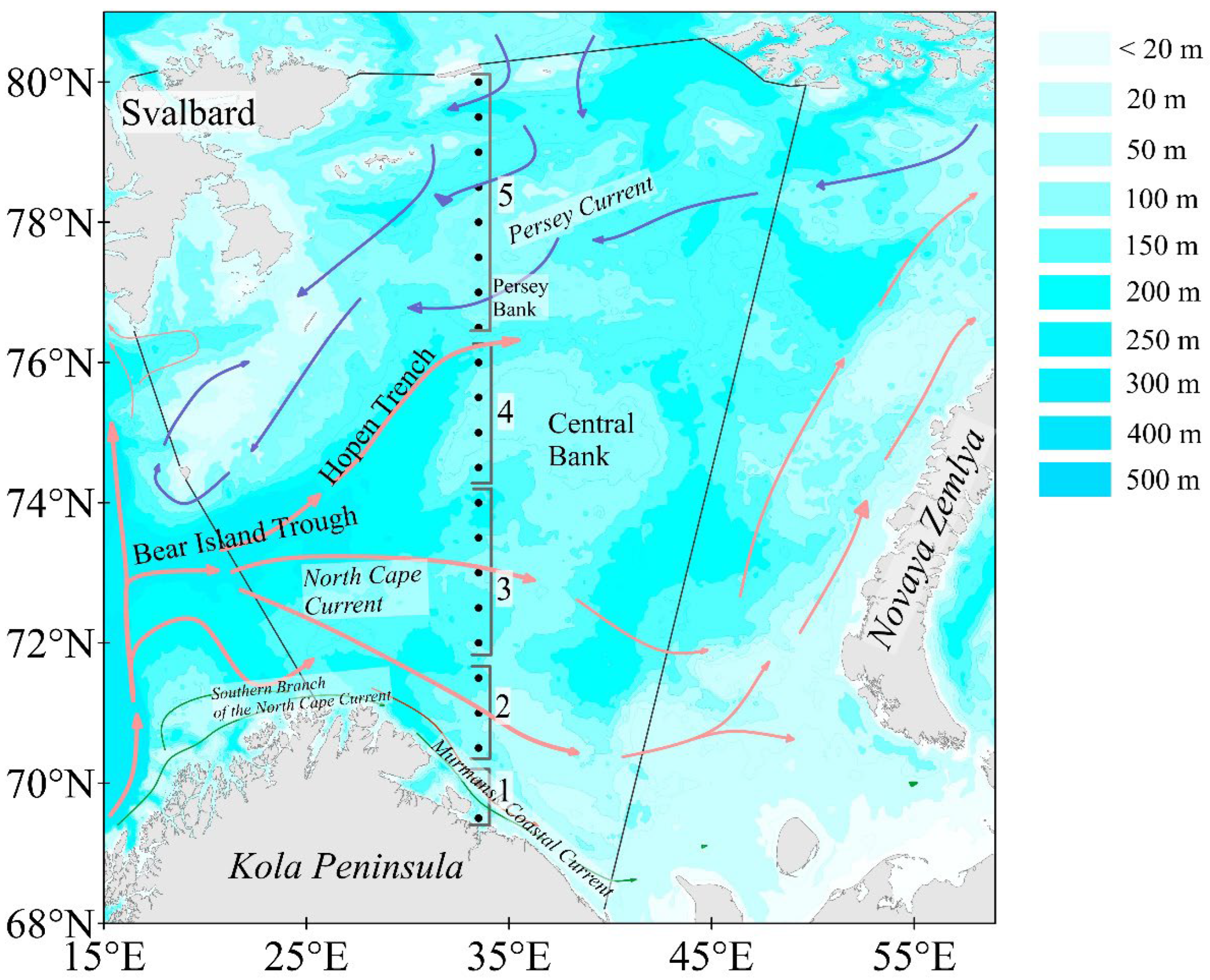
Figure 3.
Mean annual sea ice extent in the western Barents Sea from 1997 to 2023.
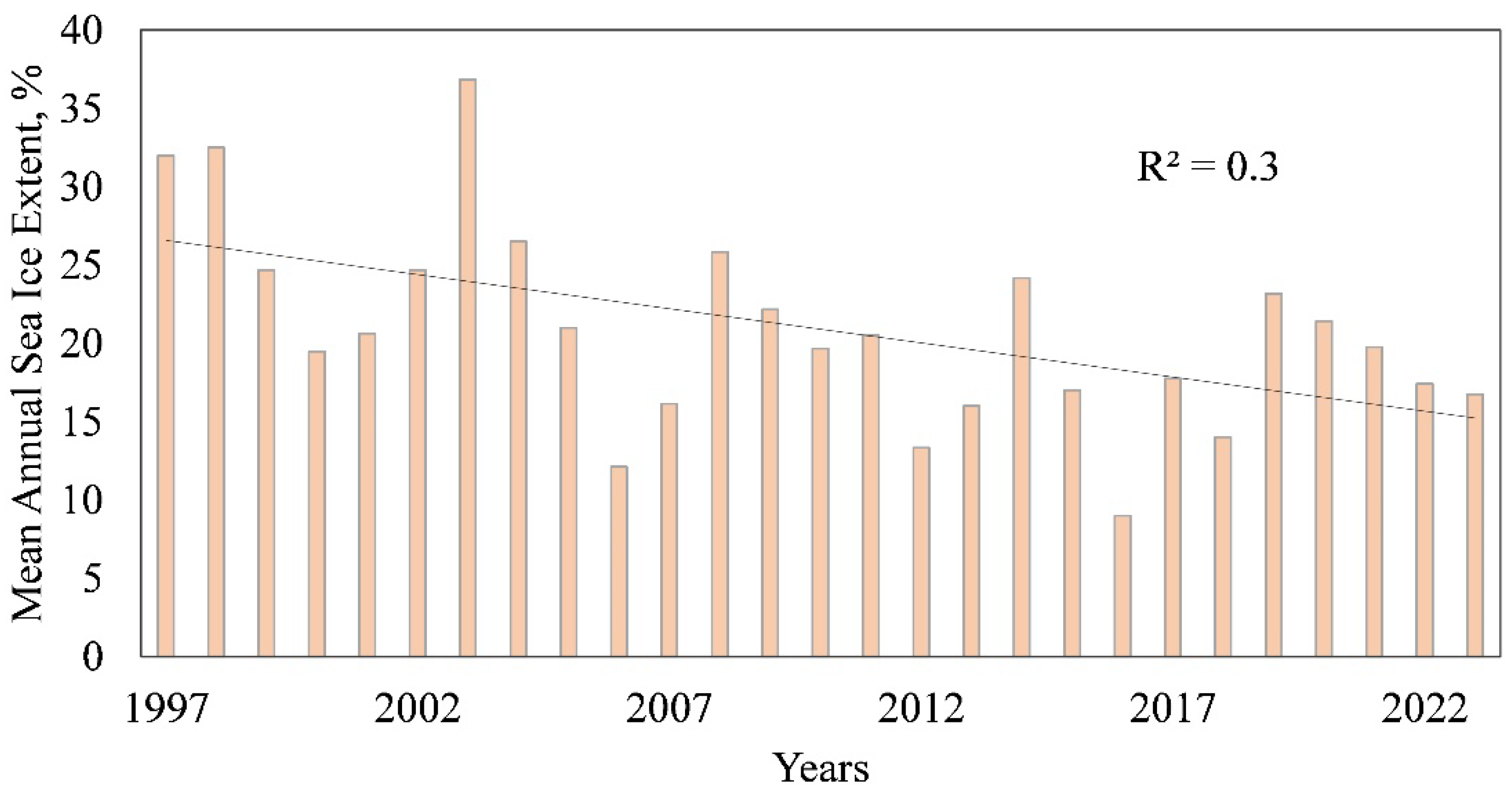
Figure 5.
Vertical distribution of temperature and salinity along the Kola Section close to average/normal background conditions in the summer of 2017. The positions of the Polar Front are highlighted with rectangular areas, and the maximum temperature gradient (∇Tmax) and salinity gradient (∇Smax) are indicated.
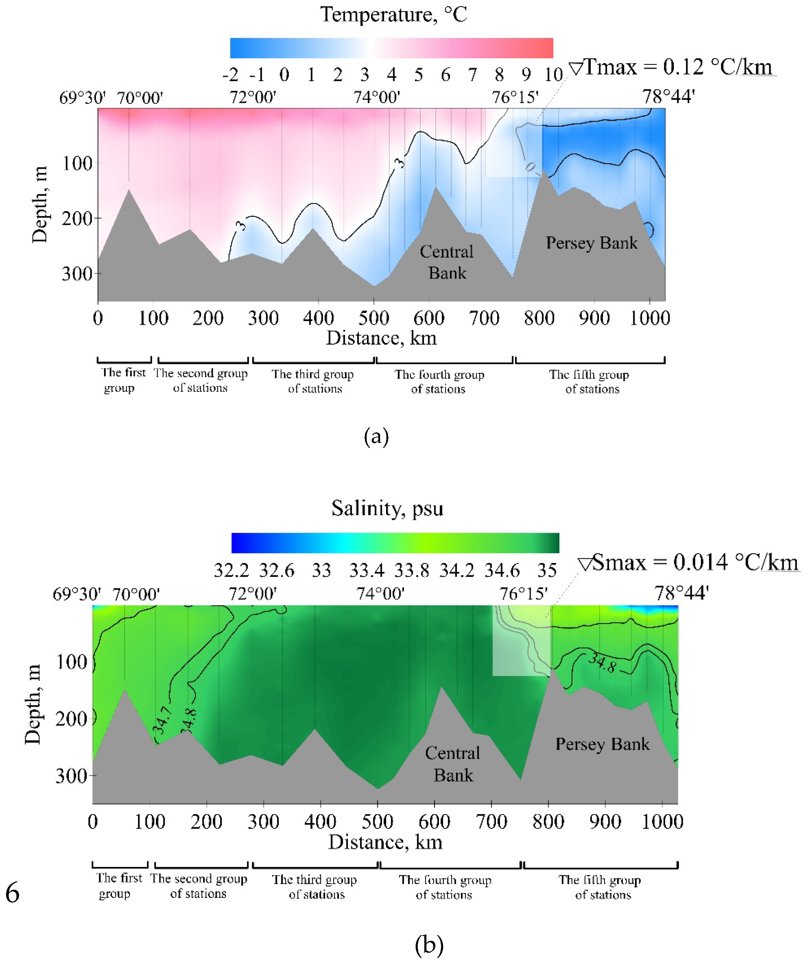
Figure 6.
Vertical distribution of temperature and salinity in the northern part of the Kola Section in 2023. The position of the ice edge is marked with a purple line. The areas of the thermal and haline components of the Polar Front are highlighted by polygons.
Figure 6.
Vertical distribution of temperature and salinity in the northern part of the Kola Section in 2023. The position of the ice edge is marked with a purple line. The areas of the thermal and haline components of the Polar Front are highlighted by polygons.
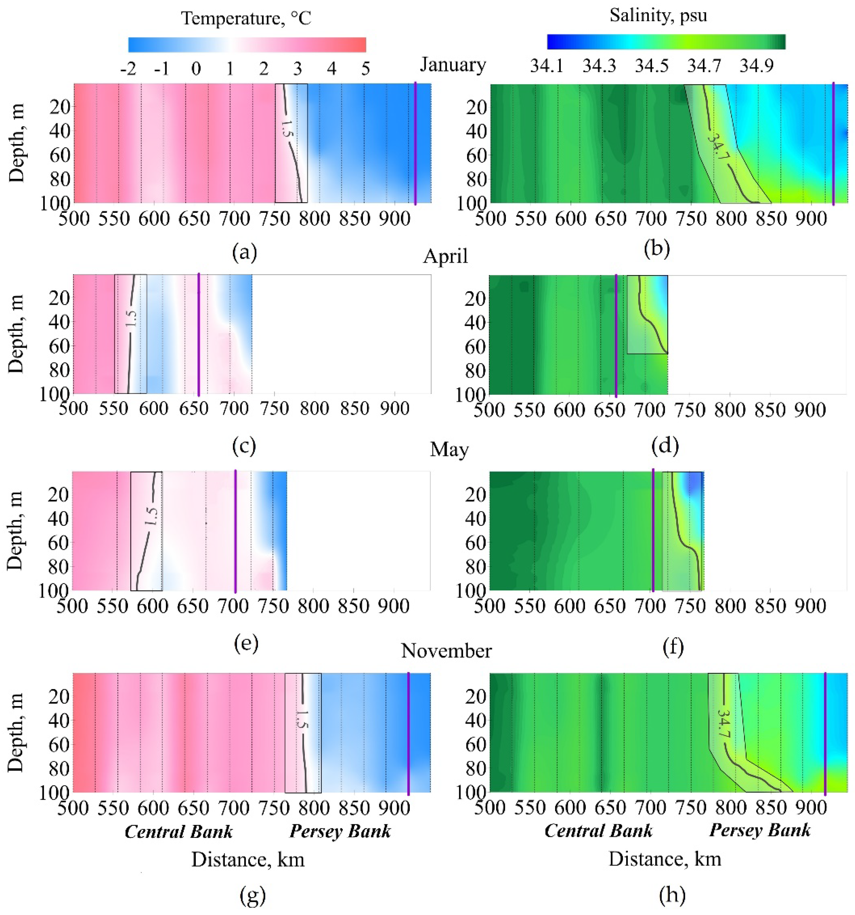
Figure 7.
Position of the 1.5°C temperature isolines (a-c) and 34.7 psu salinity isolines (d-f) along the sections for January 7-8 (a, d), April 27 (b, e), and November 26 (c, f). Dashed lines represent the positions of oceanographic stations, with blue for in situ, red for MERCATOR PSY4QV3R1, green for TOPAZ5, and yellow for CMEMS GLORYS12v1.
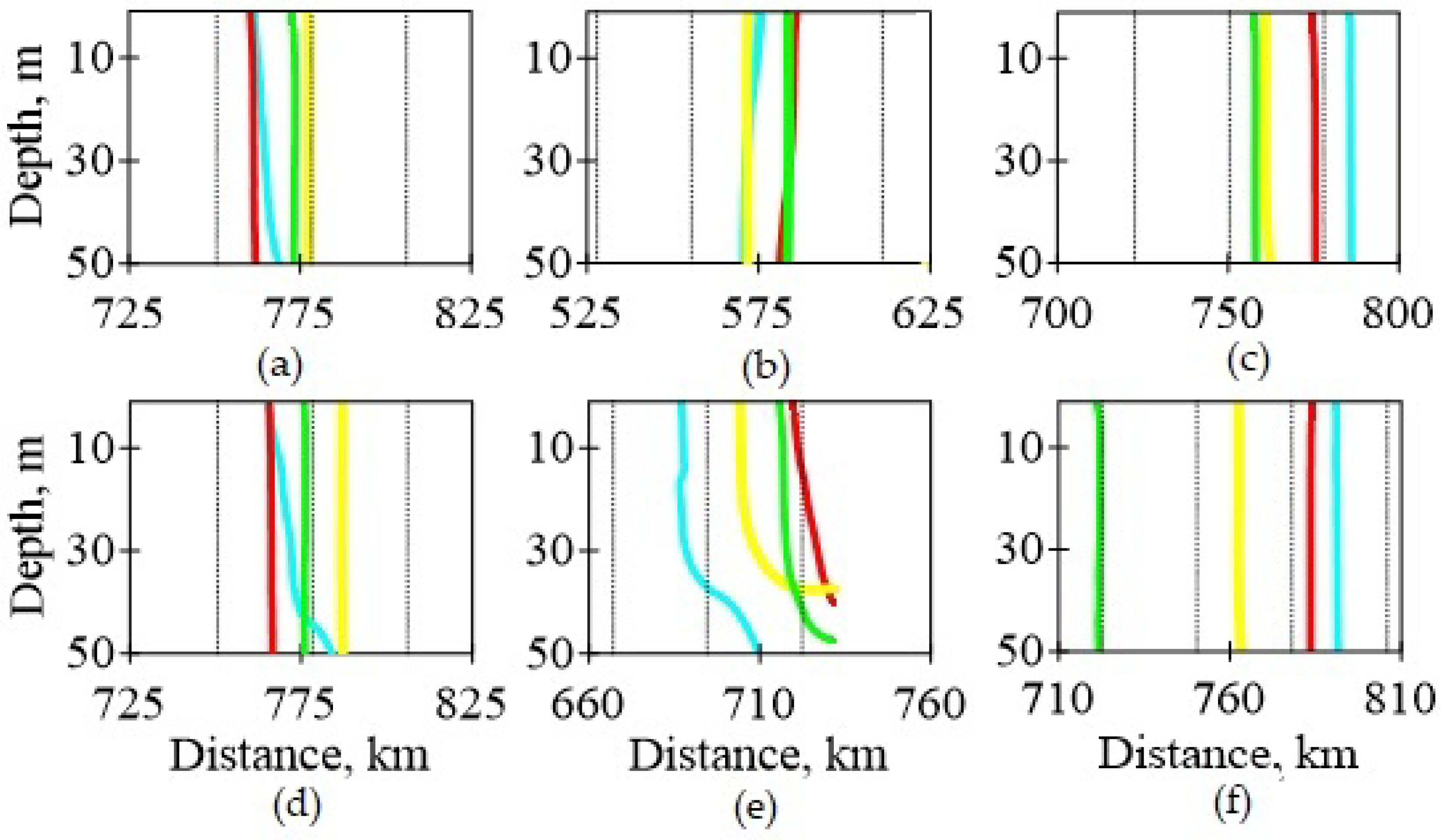
Table 1.
Description of in situ data.
| Research Dates | Number of Stations Completed | The position of the ice edge on the axis of the Kola section., N |
|---|---|---|
| 13 – 17 July 2017 г. | 28 | 78°35' |
| 29 November – 4 December 2017 г. | 35 | 79°21' |
| 14 – 16 May 2018 г. | 34 | 77°57' |
| 12 – 14 March 2022 г | 30 | 77°09' |
| 4 – 8 January 2023 | 33 | 77°55' |
| 24 – 27 April 2023 | 25 | 75°21' |
| 8 – 15 May 2023 | 23 | 75°49' |
| 20 – 26 November 2023 | 33 | 77°45' |
Table 2.
Gradations of sea ice anomalies in the western Barents Sea region and temperature anomalies along the Kola Section in the 0–50 m layer.
Table 2.
Gradations of sea ice anomalies in the western Barents Sea region and temperature anomalies along the Kola Section in the 0–50 m layer.
| Type of anomaly | Gradations of Sea Ice Anomalies, the fraction of σ | Gradations of Temperature Anomalies, the fraction of σ |
|---|---|---|
| Very strong positive anomaly (+VSA) | ΔS_ice > 1.2σ | ΔТ > 1.5 σ |
| Strong positive anomaly (+SA) | 0.4σ < ΔS_ice ≤ 1.2σ | 0.5 σ < ΔТ ≤ 1.5 σ |
| Close to average/norm (N) | ± ΔS_ice ≤ 0.4σ | ± ΔТ ≤ 1.5 σ |
| Strong negative anomaly (-SA) | 0.4σ < -ΔS_ice ≤ 1.2σ | 0.5 σ < – ΔТ ≤ 1.5 σ |
| Very strong negative anomaly (-VSA) | -ΔS_ice > 1.2σ | ؎ΔТ > 1.5 σ |
Table 4.
Values of the MHD between the positions of the isolines from in situ data and selected products, as well as the differences (An. Grad) between the weighted averages of gradients within the frontal zone based on in situ data and selected products.
Table 4.
Values of the MHD between the positions of the isolines from in situ data and selected products, as well as the differences (An. Grad) between the weighted averages of gradients within the frontal zone based on in situ data and selected products.
| Sources of the data sets being compared | January | April | November | |||
|---|---|---|---|---|---|---|
| MHD, | An. Grad, | MHD, | An. Grad, | MHD, | An. Grad, | |
| km | °C(psu)/km | km | °C(psu)/km | km | °C(psu)/km | |
| Temperature | ||||||
| In situ - MERCATOR | 2.6 | 0.045 | 8.6 | 0.037 | 10.3 | 0.028 |
| In situ – TOPAZ5 | 7.8 | 0.072 | 10.9 | 0.062 | 27.8 | 0.061 |
| In situ - GLORYS12v1 | 12.6 | 0.071 | 1.1 | 0.026 | 24.6 | 0.072 |
| Salinity | ||||||
| In situ - MERCATOR | 5.9 | -0.0003 | 26.2 | 0.0027 | 7.5 | 0.0008 |
| In situ - TOPAZ5 | 5.3 | 0.0063 | 22.1 | -0.0007 | 69.2 | 0.008 |
| In situ - GLORYS12v1 | 14.7 | 0.0075 | 11.7 | 0.0005 | 28.4 | 0.0101 |
Disclaimer/Publisher’s Note: The statements, opinions and data contained in all publications are solely those of the individual author(s) and contributor(s) and not of MDPI and/or the editor(s). MDPI and/or the editor(s) disclaim responsibility for any injury to people or property resulting from any ideas, methods, instructions or products referred to in the content. |
© 2024 by the authors. Licensee MDPI, Basel, Switzerland. This article is an open access article distributed under the terms and conditions of the Creative Commons Attribution (CC BY) license (http://creativecommons.org/licenses/by/4.0/).
Copyright: This open access article is published under a Creative Commons CC BY 4.0 license, which permit the free download, distribution, and reuse, provided that the author and preprint are cited in any reuse.


