
Submitted:
13 June 2025
Posted:
17 June 2025
You are already at the latest version
Abstract
Doppler current-meters and current profilers are currently used in oceanography to measure and record large amount of data on ocean currents. They can be vessel-mounted or standalone, single point or profiler. Calibration techniques have been experimented, described and are employed regularly for vessel-mounted or standalone equipment’s, but the uncertainties on the currents measured by these instruments are rarely estimated. This publication proposes a method based on the supplement 2 to the “Guide to the expression of uncertainty in measurement” to fill this gap. The results of simulations made by applying this method on two instruments from the best-known manufacturers, highlight a few points concerning the speed of sound, the beam slant angles from the nominal value and the application of corrections to the heading, pitch and roll angles given by the instrument, to reduce the uncertainty on the measured velocities. The method proposed in this publication can be used to simulate the uncertainties that can be expected in different configurations and different practical applications.
Keywords:
marine current
; profiler
; current-meter
; uncertainty
; Doppler effect
; compass
; tilt sensor
; mooring
1. Introduction
Subsurface currents are one of the essential climate variables defined by the Global Climate Observing System or GCOS (https://gcos.wmo.int/en/essential-climate-variables). In situ measurements can be made by Eulerian methods where instruments are on fixed moorings, or Lagrangian methods where instruments are surface or subsurface buoys ‘anchored’ in a water mass, the trajectory of which can be followed by satellites. This study concentrates on the Eulerian method where measurements are made with Doppler effect acoustic instruments that can be standalone or vessel-mounted. The assessment of uncertainties in current measurements made by these instruments, is a task that has been unsatisfactorily or at best incompletely solved to date, because of the inherent complexity of the measurement principle and also because of multiple factors contributing to the velocity uncertainty. This paper proposes a method to fill this gap.
Standalone instruments can be single-points or profilers that is to say, they can measure the velocity of water masses in a single layer or in several layers from the seabed or from the surface. They can be mounted on mooring cages deployed on the seabed or on mooring lines. On mooring lines or on the seabed they can be inclined compared to the vertical position. This inclination must be corrected to retrieve the vertical and the horizontal components of the current, and for this purpose they are equipped with tilt sensors. The direction and the amplitude of currents is retrieved at first, in the instrument body by at least three slanted beams that make a vectoral measurement of the velocity and then in the Earth framework by a matrix calculation that uses measured tilt angles and angular directions. For standalone instruments, the angular direction in relation to the magnetic North, is retrieved with a magnetic compass, and the direction in relation with the true North is retrieved by applying a correction of magnetic declination. For vessel mounted instruments, the direction and inclination are given by the inertial navigation system of the boat.
The velocity measured by standalone current-meters and current profilers can be calibrated, and an estimate of their measurement uncertainties can be made in hydrodynamic channels [1] or by carrying out inter-comparisons at sea as it was carried out in 2012 [2] or in rivers [3], but these inter-comparisons are expensive, difficult to organize, and they allow only one part of the velocity range of instruments to be tested. In addition, these two methods do not allow an estimation of errors of each sensor of the instrument separately and the calibration uncertainty can be hardly determined. In 2007 a first publication described a method to calibrate the compass of current-meters [4], and in 2014, a second publication described a method to calibrate the compass and the tilt sensors of these instruments [5] (see Figure 1). In 2020, a third publication described a method to detect the Doppler effect measurement errors made by the transducers of current-meters and profilers, and it quantified the uncertainty of this calibration [6]. It should be noted that in 2015, another method was published by von Appen to correct compass errors linked to nearby metal masses, and applied to ADCP-equipped (Acoustic Doppler Current Profiler) buoys deployed in Greenland [7]. In 2023, another publication demonstrated the impact of different elements of moorings, on the accuracy of compass measurements, and it opened the way to best practices [8].
However, if the uncertainties of direction and velocity measurements can be assessed by these techniques, a method is missing to propagate the uncertainties they quantify, on the current measurements made in situ. The “Guide to the expression of uncertainty in measurement” or GUM [9] edited by the BIPM, proposes a method based on the law of variance composition to assess a combined measurement uncertainty from a physical relation called measurement model. This model must describe the impact of the variations of input quantities on a single output quantity. The supplement 2 to the GUM [10] edited in 2011 or JCGM102: 2011, proposes a standardized method that can be applied to measurement models having any number of input and output quantities. The multi-beams Doppler current-meters and profilers respond to this kind of measurement model. Each acoustic transducer is sensitive to the same input variables and the velocities components U, V, W calculated in the earth framework are sensitive to the same measured velocities and direction quantities. The difficulty lies in the assessment of the standard uncertainties of the input variables.
This publication proposes to apply the JCGM102: 2011 method to evaluate the impact on current measurements of uncertainties on the input quantities that participate to standalone Doppler current-meters and profiler’s measurement, in the case of four-beam current profilers. Numerical applications and simulations based on two commonly used instruments, are given to validate the theoretical developments.
2. Operating Principles of Doppler Current-Meters and Profilers
Current-meters and profilers compute velocities (V1, V2, V3) obtained by Doppler shifts measurements in their beam axes (radial velocities). The transducers are tilted 20 °, 25 ° or 45 ° (angle β). β is the Janus angle or slant angle which is accurately determined by the manufacturer (Figure 2). Most of recent instruments are equipped with a fourth transducer used as rescue when the signal detection is too much degraded for one of the other beams.
Speeds (V1, V2, V3) or (V1, V2, V3, V4) are obtained after the detection of echoes resulting from the reflection of acoustic pulses on the successive layers of particles. To improve measurement trueness, pulses are repeated at a frequency fr. Some instruments can be used in narrowband or broadband mode. A narrowband instrument transmits a single tone burst and uses an autocovariance function to measure the phase or the frequency shift of the return pulses. It is worth noting that broadband techniques so that averaging improve the detection limits of pings in the noise and the profiling range of measurements or the conditions of detection in waters with low levels of particles.
The document [11] gives formulas to calculate the low limits of the velocity measurement uncertainties of narrow and broadband systems, along the beam path. For a single ping and a narrowband system, the standard deviation σNB of the horizontal velocity component can be obtained by the Formula (1):
where f0 is the transmit frequency in Hz and D the depth cell length in m. For a broadband system, the standard deviation σBB of the horizontal velocity component can be obtained by the relationship (2):
where R is the correlation at the time TL. R = 0.5 for a 2-pulses system. TL is the time separating the transmission of two pulses in a 2-pulses system and c the speed of sound. In this case, the autocorrelation function results are a major peak centred on zero and two side peaks centred on ± TL.
In order to obtain the velocities (Vx, Vy, Vz) in the referential of the instrument, manufacturers provide transfer matrix that can take different forms according to the orientation given to transducers. Figure 3 compares the enumeration of transducers and the orientation of rotation axis for the instruments Nortek Signature profiler and Teledyne RD Instruments Workhorse ADCP.
The matrix (3) can be used in the case of Nortek Signature profilers which head orientation is given in Figure 3:
In the case when the beam angle can vary independently for each beam, the angle β can be declined in different values β1, β2 or β3. For Teledyne RDI ADCP’s, this matrix takes another form. According to RDI Instruments (1998), for a convex transducer head we have:
The first three rows are the generalized inverse of the beam directional matrix representing the components of each beam in the instrument coordinate system. The last row representing the error velocity, is orthogonal to the other three rows and has been normalized so that its magnitude (root-mean-square) matches the mean of the magnitudes of the first two rows. This normalization has been chosen so that in horizontally homogeneous flows, the variance of the error velocity will indicate the portion of the variance of each of the nominally-horizontal components (X and Y) attributable to instrument noise (short-term error). If one beam is marked bad due to low correlation or fish detection, then a three-beam solution is calculated by the ADCP. If, for example, the beam 4 is bad, the term is replaced by a 0 value which is equivalent to a 3-beam solution.
Current-meters are equipped with ‘flux-gate’, ‘Hall effect’ or magneto-resistive compasses to retrieve the amplitude of current components (U, V, W) in reference to the magnetic North (angle α), and considering the magnetic declination at the place of measurements, in relation to the true North. Moreover, their inclination is corrected thanks to a tilt sensor measuring roll angles θ and pitch angles Ψ. For vessel-mounted instruments, these data come from the attitude sensors of the boat. According to [12], between 1 and 12 equations can be found to describe a rotation in the three dimensions.
Concerning the reference frame given in Figure 3 for the Nortek instruments, a Nortek routine called “signatureAD2CP_beam2xyz_enu.m” (https://support.nortekgroup.com/hc/en-us/articles/360029820971-How-is-a-coordinate-transformation-done?) can be used to calculate a rotation matrix for instruments in the Signature range. That gives:
Teledyne RD Instruments describes an inverse rotation matrix to retrieve the values of components (U, V, W), in its document of 1998, upgraded in 2010 [13]. For profilers installed on boats, they use the names starboard S, forward F, and mast M, instead of pitch, roll, and heading for the axes. If the beam 3 is aligned with the keel on the forward side of the ADCP, for the downward-looking orientation, these axes are identical to the instrument axes: S = X, F = Y, M = Z. For the upward-looking orientation, S = -X, F = Y, M = -Z. In earth coordinates, the roll, pitch, and heading angles correspond to Y axis, X axis andZaxis(downward looking). This description corresponds to the right schematic of Figure 3. To retrieve the components (U, V, W), they use the following rotation matrix [6]:
Velocities V1, V2, V3 and V4 of matrix (3) and (4) are obtained after the detection of echoes resulting from the reflection of pulses on successive layers of particles that are carried along by the currents. This displacement creates a frequency shift δfi (i ∈{1, 2, 3, 4}) called Doppler shift. Echoes are measured continuously, allowing the size of measurement cells in the water column to be determined (Figure 2), considering the value of the speed of sound in seawater c and the duration tp of pulses. The lowest uncertainty that can be obtained for the measurements of (V1, V2, V3, V4) is limited by the standard deviation of the Doppler noise σδ, which is inversely proportional to tp. This noise is generated by the random displacement of particles, the multiple echoes and the detection limits of the instrument electronics. Different techniques exist to extract the signal from the noise and to improve the detection limit (see [14], or [15], or [11], or [16]). If f0 is the emitted frequency, the measured radial velocity is obtained by the Doppler effect relationship:
In this relation, c is programmed in the instrument by the user or calculated by a relation using temperature, pressure measurements and sometimes a value of practical salinity.
3. Method to Evaluate the Currents Measurements Uncertainties
3.1. Uncertainties on the Instrument Body Velocities
It is necessary to consider at first, the matrix (3) and (4) that allow to transform the measured velocities (V1, V2, V3, V4) in the instrument body velocities (Vx, Vy, Vz, Ve). β is affected by a manufacturing uncertainty. Manufacturers never communicated about this uncertainty but they characterize to the best each type of instrument’s head to obtain a unique transformation matrix. The remaining uncertainty is given to be included in the accuracy given in the specification sheet established by the manufacturer. This uncertainty will be called uβ. The sensitivity of this uncertainty can be evaluated thanks to the matrix products (3) or (4). For example, considering a Nortek Signature 500 kHz where β = 25 °, if V1 = -1 m/s, V2 = 1 m/s, V3 = - 5 m/s and V4 = 5 m/s, Vx value changes of 0.018 m/s, Vy of 0.004 m/s, Vz of 0.001 m/s and per 0.1 ° in error. The measurement range of this instrument is ± 5 m/s along the beams. Therefore, its maximal sensitivity to the slant angle is 0.18 m/s/° (see Table 1).
The same simulation can be made on a Teledyne RD Instrument Workhorse Sentinel 600 kHz. On this instrument, β = 20 °. In order to obtain instrument body velocities less than 5 m/s to compare calculated values with the Signature values, it is necessary to take V1 = 4.4 m/s, V2 = 1 m/s, V3 = 3.3 m/s and V4 = 1 m/s. In this case, Vx value changes of 0.024 m/s, Vy of 0.023 m/s, Vz of 0.001 m/s and per 0.1 ° in error. Therefore, its sensitivity at 5 m/s to the slant angle is 0.24 m/s/°. A reduced slant angle increases the sensitivity to the manufacturing tolerance on this angle.
Velocities (V1, V2, V3, V4) measured from the Doppler effect, have three sources of uncertainties:
- the first comes from the accuracy in which this effect is measured by the instrument. It is dependent on the linearity of its electronic or on the stability of its oscillator. This part can be evaluated during the calibration of transducers as described in [6]. It participates to the uncertainty uδf.
- The second comes from the conditions of reflection in the medium and of the detection techniques employed. This part also participates to the uncertainty uδf, and it is hard to assess. If pings average are made, some instruments can also generate a standard deviation per measurement cell to quantify the uncertainty of Doppler shifts real-time measurement. In this case, the resulting standard deviation can be quadratically add to the transducer’s calibration uncertainty.
- The third source depends on the difference between the speed of sound programmed in the instrument, and the true speed of sound in the medium. It can be evaluated thanks to Formula (7). Considering that f0 is perfectly determined, and that c has an uncertainty uc on its determination, as δfi and c are two independent quantities, we can write that the uncertainty uvi on Vi is:
Considering again a Signature 500 kHz, if 1500 m/s is programmed in the instrument and the true velocity is unknow but estimated to be inferior to 1520 m/s, according to BIPM (2008), or 11.5 m/s. If Vi = 1 m/s, for f0 = 500 kHz, δfi = 758 Hz. The uncertainty on the calibration of transducers is generally close to 0.002 m/s, what makes uδf = 1.6 Hz. In this case, the first member of the Equation (8) is 4 10-6 and the second member is 5.8 10-5. The uncertainty on the speed of sound dominates largely the uncertainty on the measured velocity. For Vi = 1 m/s, the uncertainty on Vi is 0.008 m/s or 0.76 % of the measured speed. This uncertainty decreases as Vi increases.
From a measurement point of view, velocities (V1, V2, V3, V4) are determined independently, in the same layer of water. However, there is a spatial correlation between the beams due to their angle of inclination. Their covariance is proportional to the cosine of the slant angle. If the slant β was 90 °, cov(Vi, Vj) = 0 pour i # j ∈ {1, 2, 3, 4}. Therefore, it is possible to estimate the covariance of Vi’s by the relation: cov(Vi, Vj) = uVi uVj cos(β), to form the variance matrix Vvi, which diagonal is composed of the squared of the standard uncertainties uVi of the velocities Vi, i ∈ {1, 2, 3, 4}. Vvi has the form:
where cij = cov(Vi, Vj) i # j ∈ {1, 2, 3, 4}. β is a variable independent of Vi, i ∈ {1, 2, 3, 4}. The uncertainty on the speeds (Vx, Vy, Vz) of matrix (3) or (4) can be obtained, according to [10], from the matrix product (10):
Vx, Vy, Vz and Ve are functions of V1, V2, V3, V4 and β. In the case of a 4-beam ADCP, M will take the form:
MT is the transposed matrix of M. The derivatives of Vx, Vy, Vz and Ve with respect to V1, V2, V3, V4 correspond to the elements of matrix (3) or (4) according to the chosen ADCP. The derivatives of Vx, Vy, Vz and Ve with respect to β can be obtained with the Equations (12) and (13):
Equation (12) can be used for the matrix (3) and the following Equation (13) can be used for the matrix (4):
It is well known that ADCP do not provide reliable water velocity measurements near the sea surface or near the bottom, because acoustic sidelobe reflections from the boundary contaminate the Doppler velocity measurements [17]. For the surface, the bias will depend on the sea state or surface wind conditions. Higher velocities are measured in the upper layer. In 2022, Lentz et al. formulated a relationship suggesting that the contaminated region is deeper than traditionally suggested, with a dependence on the bin size Δz [18]. The depth zsl was calculated with the relationship zsl = ha[1 - cos(β)], where ha is the distance from the ADCP acoustic head to the sea surface. According to [18], the true depth z of this region must be assessed with the relation: z < zsl + 3Δz/2. However, this publication does not provide a method or a relationship for assessing the magnitude of the error or of the uncertainty on the measured velocity as a function of depth, and there is no way in post-processing to separate the bias effect of side-lobes. Consequently, the measurements made in a depth inferior to z are excluded of the field of our publication.
3.2. Uncertainties on Velocities Calculated in the Earth Framework
The determination of U, V and W just requires 3 beams. Let us consider that the measurements of Vx, Vy, Vz are of a good quality and that Ve is not required. In the same way, U, V and W of matrix (5) and (6), are determinist functions of 6 independent variables Vx, Vy, Vz, α, θ and that have measurement uncertainties uvx, uvy, uvz, uα, uθ, . That gives the diagonal variance matrix V6v:
The uncertainties on the speeds (U, V, W) of matrix (5) or (6) can be obtained with the product:
with:
MfT is the transposed matrix of Mf. The equations of derivatives of the matrix (15) applied to the matrix (5) and (6), are given in the supplementary materials.
4. Numerical Applications and Results
There are so many different current-meters and current profilers and so many ways of configuring and using them, that it is impossible to obtain a unique numerical result representing the measurement uncertainty that can be expected from these instruments. In order to see how the relationships of the section 3 can be applied and in order to give an order of magnitude of the final uncertainties that can be found, numerical applications have been made based on a Nortek Signature 500 kHz and on a 600 kHz RD Instrument Workhorse Sentinel. These instruments have frequencies in the average of the frequency range of the commercially available instruments and they are widely used in oceanography.
The Nortek Signature 500 kHz has a slant angle β = 25 °. The uncertainty uβ on the determination of this slant angle is unknown, but the standard ISO 2768 [19] determines classes of tolerances on angles in mechanical parts manufacturing. The higher class allows to define angles to 0° 5′ or 0.083 ° (0.0014 rad). This value will be taken as an example to define the uncertainty uβ, but without any real knowledge of what can be obtained by manufacturers.
With V1 = -1 m/s, V2 = 1 m/s, V3 = - 5 m/s and V4 = 5 m/s, we have uV1 = uV2 = 0.008 m/s, and uV3 = uV4 = 0.039 m/s by considering a maximal uncertainty of 20 m/s on the speed of sound c. That gives the matrix:
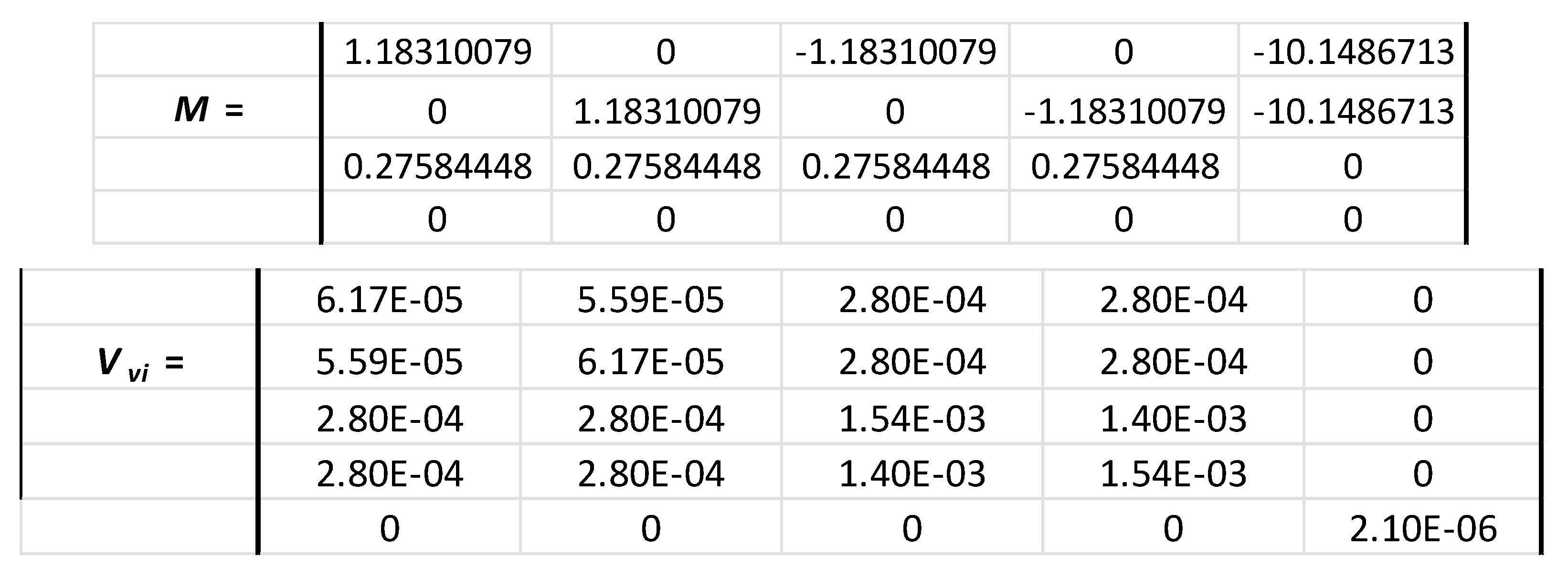
and uVx = uVy = 0.041 m/s, and uVz = 0.025 m/s, with Vx = 4.732 m/s, Vy = 1.183 m/s and Vz = - 1.379 m/s. If we consider now that β is perfectly determined and has no uncertainty, the values of uVx and uVy become a little bit smaller: uVx = uVy = 0.038 m/s, and we have always uVz = 0.025 m/s. Therefore, this calculation shows that the uncertainties on the measured speeds are slightly sensitive to the slant angle of beams and that the smallest uncertainty allowed on the manufacturing has a small impact on the horizontal measured velocities. That highlights the necessity for manufacturers to compensate it with adjusted values of β in matrix (3) and (4), and to communicate about it.
If the heading, roll and pitch angles are taken to be 0 °, U = Vx, V = Vy and W = Vz. Using the calibration platform described in [8] or [5], the typical standard uncertainties that can be obtained on heading, roll and pitch angles are: uα = 0.59 °, uθ = 0.21 ° and = 0.22 °. That gives the matrix:
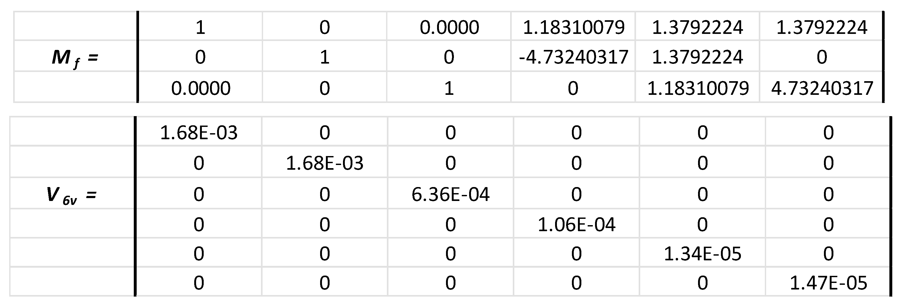
The relationship (15) gives uU = 0.043 m/s, uV = 0.064 m/s and uW = 0.021 m/s. In the case when uβ = 0 °, uU = 0.041 m/s, uV = 0.062 m/s and uW = 0.021 m/s.
If now the profiler is turned by α = 70 ° and tilted by θ = = 5 °, the values of U, V and W are different (U = 2.87 m/s, V = - 4.09 m/s and W = - 0.85 m/s) so that their measurement uncertainties: uU = 0.059 m/s, uV = 0.051 m/s and uW = 0.032 m/s. If uβ = 0 °, uU = 0.057 m/s, uV = 0.048 m/s and uW = 0.032 m/s.
Bias are often found on compass and tilt sensors after several years of using. Let us suppose that these biases are not corrected and considered as uncertainties, and that uα = 6 °, uθ = 1 ° and = 1 ° which are error values currently found. In this case, the calculation gives: uU = 0.43 m/s, uV = 0.30 m/s and uW = 0.09 m/s. If uβ = 0 °, the uncertainties remain the same: uU = 0.43 m/s, uV = 0.30 m/s and uW = 0.09 m/s. The uncertainties on U and V are very large and dominated by the compass uncertainty. They represent 15 % and 7 % of the measured value. To check their trueness, we just need to look at how U, V and W vary when α, θ and go respectively from 70 ° to 76 ° and from 5 ° to 5.8 °. The differences obtained by using the matrix (5) is δU = 0.42 °, δV = 0.28 ° and δW = 0.08 ° which is very close of values found for uU, uV and uW.
This simulation shows the importance of correcting the compass and tilt sensors errors to make these uncertainties equivalent to the calibration uncertainties. All these results are resumed in Table 2.
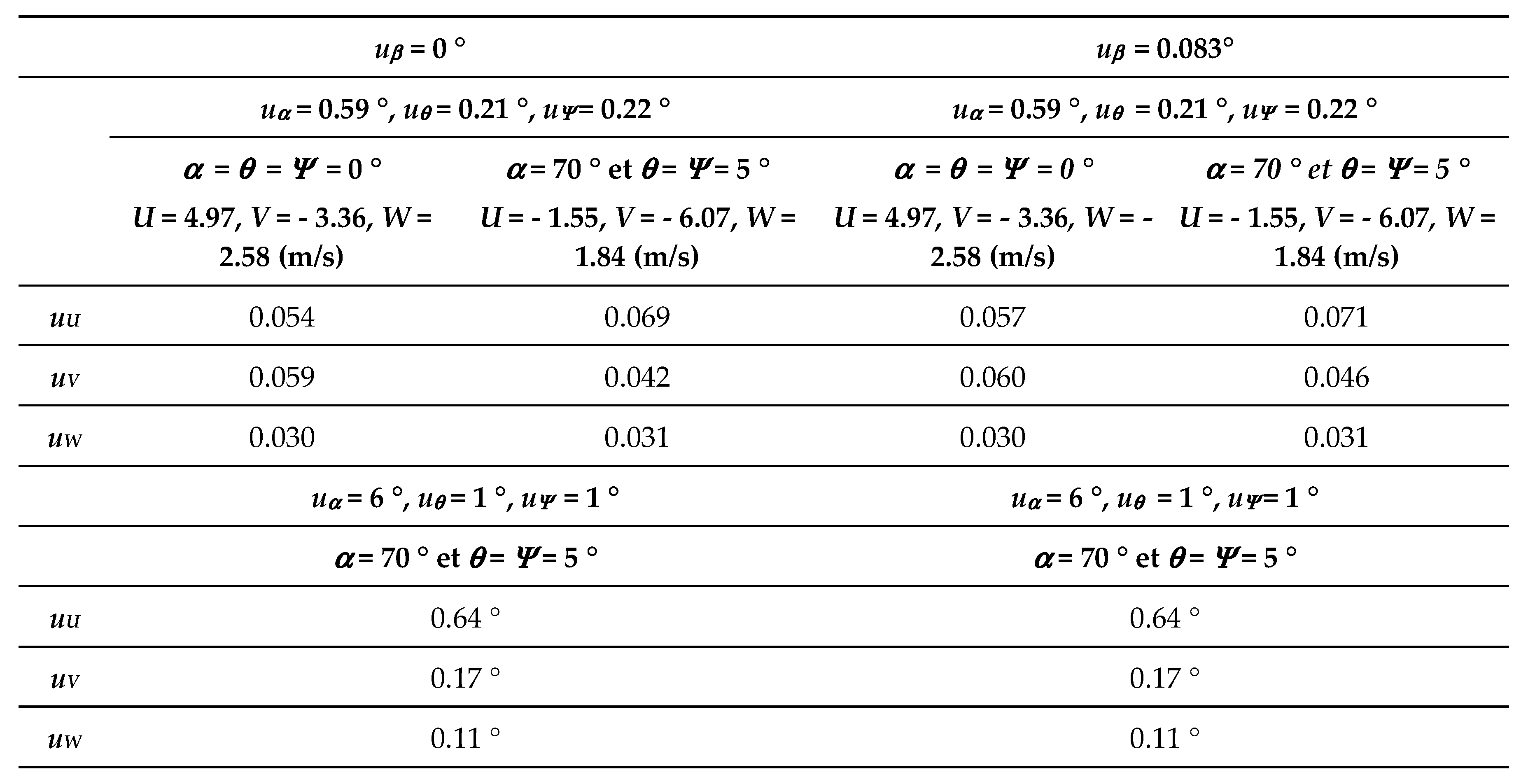
The same numerical applications can be made on RD Instrument Workhorse Sentinel. The specifications of the 600 kHz are the closest of the 500 kHz Signature. For this instrument, β = 20 °. With V1 = 4.4 m/s, V2 = 1 m/s, V3 = 3.3 m/s and V4 = 1 m/s, we have uV1 = 0.036 m/s, uV3 = 0.026 m/s, and uV2 = uV4 = 0.008 m/s by considering again a maximal uncertainty of 20 m/s on the speed of sound c. That gives the matrix:
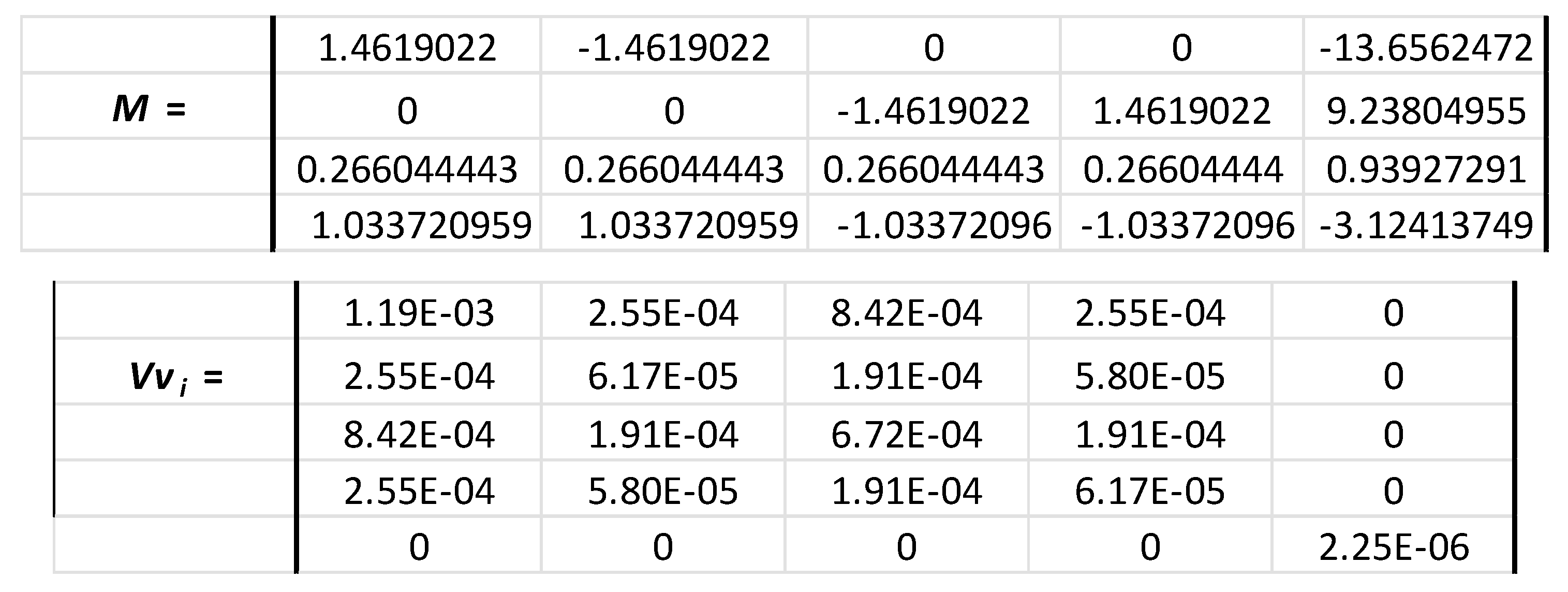
and uVx = 0.045 m/s, uVy = 0.030 m/s, uVz = 0.020 m/s and uVe = 0.015 m/s, with Vx = 4.97 m/s, Vy = - 3.36 m/s, Vz = 2.58 m/s and Ve = 1.14 m/s. If we consider now that β is perfectly determine and has no uncertainty, like for the Signature, the values of uVx, uVy are smaller and uVz is unchanged: uVx = 0.040 m/s, uVy = 0.027 m/s, uVz = 0.020 m/s and uVe = 0.014 m/s.
If the heading, roll and pitch angles are taken to be 0 °, U = Vx, U = Vy and W = Vz. Using the previous heading, roll and pitch uncertainty values (uα = 0.59 °, uθ = 0.21 ° and = 0.22 °), that gives the matrix:
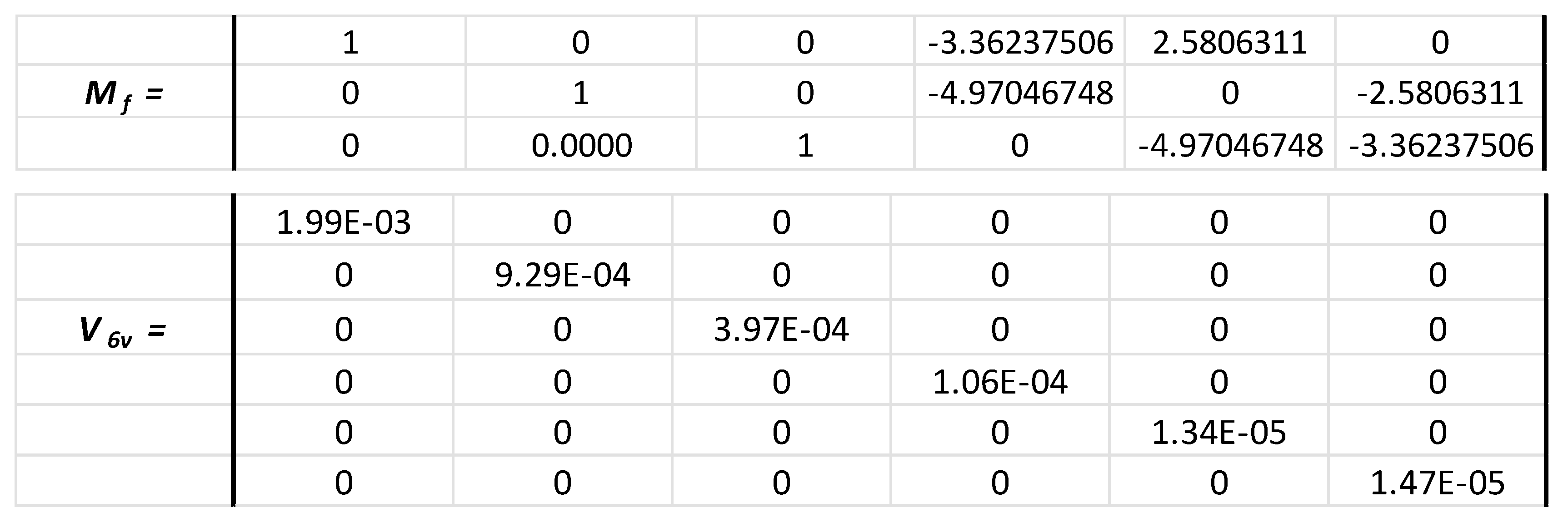
We have again uU = 0.057 m/s uV = 0.060 m/s but uW = 0.030 m/s. In the case when uβ = 0 °, uU = 0.054 m/s, uV = 0.059 m/s and uW = 0.030 m/s. These values are of the same order of magnitude as those obtained with the Signature.
If now the profiler is turned by α = 70 ° and tilted by θ = = 5 °, the values of U, V and W are different (U = - 1.55 m/s, V = - 6.07 m/s and W = + 1.84 m/s) and the uncertainties on U, V and W are distributed differently: uU = 0.071 m/s, uV = 0.046 m/s and uW = 0.031 m/s. If uβ = 0 °, uU = 0.069 m/s, uV = 0.042 m/s and uW = 0.031 m/s.
Let us suppose again that uα = 6 °, uθ = 1 ° and uΨ = 1 ° which are error values currently found. In this case, the calculation gives: uU = 0.637 m/s, uV = 0.172 m/s and uW = 0.112 m/s. If uβ = 0 °, uU = 0.637 m/s, uV = 0.170 m/s and uW = 0.112 m/s. The uncertainties on U and V are again very large and dominated by the compass uncertainty. They represent respectively 41 %, 3 % and 6 % of the measured value. To check their trueness, we just need to look at how U, V and W vary when α, θ and go respectively from 70 ° to 76 ° and from 5 ° to 5.8 °. The differences obtained by using the matrix (6) is δU = 0.64 °, δV = 0.16 ° and δW = 0.13 ° which is very close of values found for uU, uV and uW. All these results are resumed in Table 3. This simulation demonstrates again the importance of correcting the compass and tilt sensors errors to make these uncertainties equivalent to the calibration uncertainties.
In order to illustrate the possibilities of simulation offered by this method, four graphs have been plotted (Figure 4, Figure 5 and Figure 6). The first one (Figure 4) shows the evolution of U, V and W uncertainties when the uncertainty on the heading increases from 0 to 10 °, for the values used in Table 1: α = 70 ° and θ = Ψ = 5 °, U = 2.87 m/s, V = - 4.09 m/s, W = - 0.85 m/s, uθ = 0.21 °, uΨ = 0.22 °. As expected, uW remains constant and uU and uV increase linearly.
The second one, (Figure 5) shows the evolution of U, V and W uncertainties when the uncertainties on the roll and pitch measurements increase of the same value from 0 to 4 °, again for the values used in Table 1: α = 70 ° and θ = Ψ = 5 °, U = 2.87 m/s, V = - 4.09 m/s, W = - 0.85 m/s, uα= 0.59 °. As expected, the uncertainties on U and V evolve moderately and the uncertainty on W increases linearly.
To quantify the effect of a large uncertainty on the speed of sound, we have plotted the evolution of the uncertainties in V1, V2 and V3 (Figure 6a) and the evolution of the uncertainties in U, V and W, as a function of the uncertainty in c (Figure 6b). When the relative uncertainty uVi/Vi increases from 0.2 to 3.3 % as uc increases from 0 to 50 m/s, the relative uncertainty uU/U increases from 1.2 % to 5.7 %, which corresponds to a 4.5 % increase, and uW/W increases from 2.3 % to 12.8 %, which corresponds to a 10.5 % increase.
5. Conclusions
Doppler effect current meters and profilers are technologically complex measuring instruments. They enable massive quantities of data to be collected on marine currents, but the complexity of their operation has always been an obstacle to a rigorous assessment of the uncertainties of their measurements. The method described in this publication takes into account all the elements involved in calculating the amplitude and direction of currents and the restitution made by the software of the instrument that rest on using of a transfer and a rotation matrix. This functioning responds to the method described in the Supplement 2 to the “Guide to the expression of uncertainty in measurement” edited by the BIPM [10].
Applying this method with available values of uncertainties, allows us to highlight a few important points:
- for velocities (V1, V2, V3, V4) resulting directly from the Doppler shift measurements, the uncertainty coming from a bad knowledge of the speed of sound c at the place of measurements is much greater than that on the measurement of the Doppler shift. The determination of this value is often neglected so that it can impact the measured velocity from 0.2 to 3.3 % for an uncertainty on c that vary from 0 to 50 m/s, and this impact on U, V and W components is still more important.
- The beams slant angle of ADCPs is an important element that participates to the final uncertainty on the amplitude of currents components. This is ignored in instruments specifications sheets.
- However, the compass and tilt sensors effects are the more influent sources of uncertainties. The compass errors can be the result of elements like battery packs that create magnetic anomalies or other devices as showed in [8]. As they often are ignored or not precisely quantified, they become sources of uncertainties.
The method proposed in this publication can be used to simulate the uncertainties that can be expected in different configurations and different practical applications.
Data availability
no new data were created or analyzed in this study. Data sharing is not applicable to this article.
Supplementary Materials
The following supporting information can be downloaded at the website of this paper posted on Preprints.org. The equations of derivatives of the matrix (16) applied to the matrix (5) RD Instrument and (6) Nortek, can be downloaded at: https://www.mdpi.com/article/doi/s1.
Author Contributions
MLM is the first authorship. CC contributed in the redaction and the correction of the document, JV contributed to the verification of numerical values.
Funding
This paper was written in the frame of the MINKE (Metrology for Integrated Marine Management and Knowledge-Transfer Network) Project funded by the European Commission within the Horizon 2020 (2014-2020) research and innovation program under grant agreement 101008724.
Conflicts of Interest
The authors declare that the research was conducted in the absence of any commercial or financial relationships that could be construed as a potential conflict of interest.
References
- Camnasio, E. and Orsi, E. Calibration Method of Current Meters. J. Hydraul. Eng. 2011, 137, 386–392. [Google Scholar] [CrossRef]
- Drozdowsky, A.; Greenan, B. J. W. An Intercomparison of Acoustic Current Meter Measurements in Low to Moderate Flow Regions. J. Atmos. Ocean. Technol. 2013, 30, 1924–1939. [Google Scholar] [CrossRef]
- Boldt, J.A.; Oberg, K.A. Validation of streamflow measurements made with M9 and RiverRay acoustic Doppler current profilers. J. Hydraul. Eng. 2015, 142, 2. [Google Scholar] [CrossRef]
- Le Menn, M.; Le Goff, M. A method for absolute calibration of compasses. Meas. Sci. Technol. 2007, 18, 1614–1621. [Google Scholar] [CrossRef]
- Le Menn, M.; Lusven, A.; Bongiovanni, E.; Le Dû, P.; Rouxel, D.; Lucas, S. and Pacaud, L. Current profilers and current meters: compass and tilt sensors errors and calibration. Meas. Sci. Technol 2014, 25, 085801. [Google Scholar] [CrossRef]
- Le Menn, M. and Morvan, S. Velocity Calibration of Doppler Current Profiler Transducers. J. Mar. Sci. Eng. 2020, 8, 847. [Google Scholar] [CrossRef]
- Von Appen, W.-J. Correction of ADCP errors resulting from iron in the instrument’s vicinity. J. Atmos. Ocean. Technol. 2015, 32, 591–602. [Google Scholar] [CrossRef]
- Le Menn, M.; Lefevre, D.; Schroeder, K.; Borghini, M. Study of the origin and correction of compass measurement errors in Doppler current meters. Front. Mar. Sci. 2023, 10, 1254581. [Google Scholar] [CrossRef]
- BIPM, JCGM 100:2008. Evaluation of measurement data – Guide to the expression of uncertainty in measurement. GUM 1995 with minor corrections, 2008.
- BIPM, JCGM 102:2011. Evaluation of measurement data – Supplement 2 to the “Guide to the expression of uncertainty in measurement”- Extension to any number of output quantities, 2011.
- RD Instrument. Field Service Technical Paper 001 (FST-001) Broadband ADCP Advance Principles of Operation, 1996. https://www.teledynemarine.com/en-us/support/SiteAssets/RDI/Technical%20Notes/FST%20Documents/FST001.PDF.
- Wertz, J. R. Spacecraft attitude determination and control, Kluwer Academic Press, 1978. [CrossRef]
- RD Instrument. ADCP Coordinate Transformation, Formulas and calculation, 1998. https://www.teledynemarine.com/en-us/support/SiteAssets/RDI/Manuals%20and%20Guides/General%20Interest/Coordinate_Transformation.pdf.
- Dillon, J.; Zedel, L.; Hay, A. E. Simultaneous Velocity Ambiguity Resolution and Noise Suppression for Multifrequency Coherent Doppler Sonar, J. Atmos. Ocean. Technol. 2012, 29, 450–463. [Google Scholar] [CrossRef]
- Lohrmann, A.; Hackett, B.; Roed, L. P. High resolution measurements of turbulence, velocity and stress using a pulse-to-pulse coherent sonar, J. Atmos. Ocean. Technol. 1990, 7, 19–37. [Google Scholar] [CrossRef]
- Nortek manuals. The comprehensive manual for ADCP’s, 2017. https://support.nortekgroup.com/hc/en-us/article_attachments/6038163404828.
- Appell, G. F.; Bass, P. D. and Metcalf, M. A. Acoustic Doppler current profiler performance in near surface and bottom boundaries. IEEE J. Oceanic Eng. 1991, 16, 390–396. [Google Scholar] [CrossRef]
- Lentz, S. J.; Kirincich, A. and Plueddemann, A. J. A Note on the Depth of Sidelobe Contamination in Acoustic Doppler Current Profiles. J. Atmos. Ocean. Technol. 2022, 39, 31–35. [Google Scholar] [CrossRef]
- ISO 2768-1:1989. Tolérances générales. Partie 1: Tolérances pour dimensions linéaires et angulaires non affectées de tolérances individuelles. https://www.iso.org/fr/standard/7748.html.
Figure 1.
Example of an RD Instrument ADCP attached on a mooring cage placed on a compass calibration platform.
Figure 1.
Example of an RD Instrument ADCP attached on a mooring cage placed on a compass calibration platform.
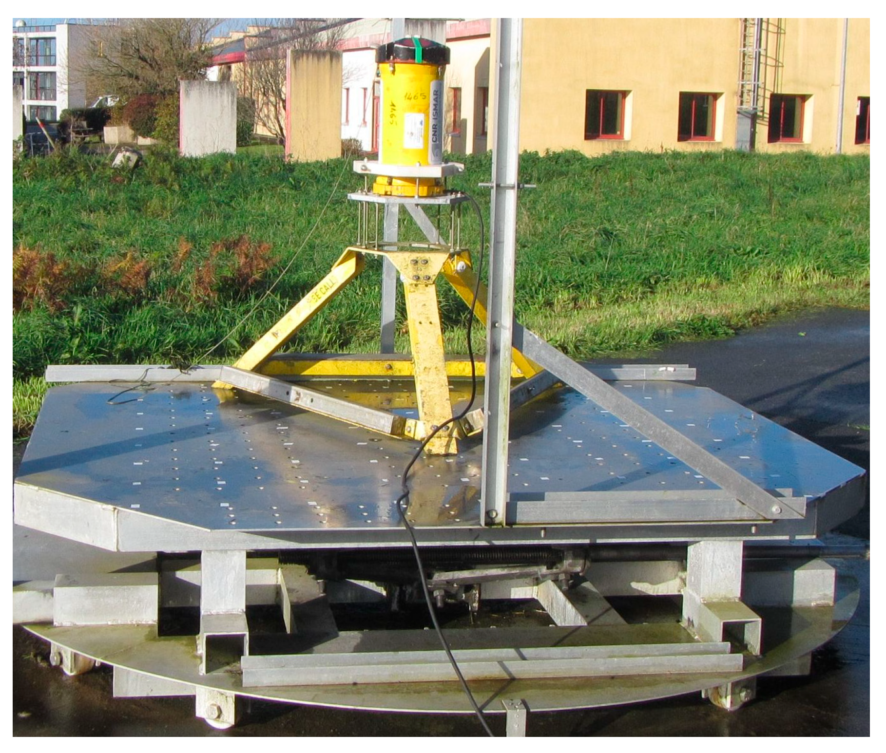
Figure 2.
Schematic of the beams of an ADCP with the velocities V1, V2, V3 calculated in the beams axis and the transducers’ slant angle β. The virtual measurement cells where the velocities are calculated, are also represented in each beam.
Figure 2.
Schematic of the beams of an ADCP with the velocities V1, V2, V3 calculated in the beams axis and the transducers’ slant angle β. The virtual measurement cells where the velocities are calculated, are also represented in each beam.
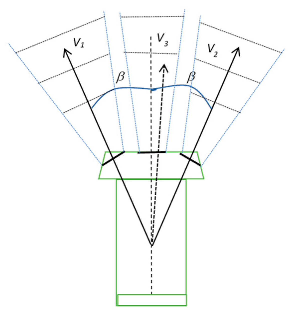
Figure 3.
On the left, beam enumeration and orientation of a Nortek Signature profiler and on the right, beam enumeration and orientation of Teledyne RD Instruments Workhorse ADCP. In the Teledyne configuration, the Z axis points away from the transducers to the pressure case, so that in the Nortek configuration, it points away from the transducer to the water.

Figure 4.
Evolution of U, V and W uncertainties when the uncertainty on the heading increases from 0 to 10 ° for the values used in Table 1: α = 70 ° et θ = Ψ = 5 °, U = 2.87 m/s, V = - 4.09 m/s, W = - 0.85 m/s, uθ= 0.21 °, uΨ = 0.22 °.
Figure 4.
Evolution of U, V and W uncertainties when the uncertainty on the heading increases from 0 to 10 ° for the values used in Table 1: α = 70 ° et θ = Ψ = 5 °, U = 2.87 m/s, V = - 4.09 m/s, W = - 0.85 m/s, uθ= 0.21 °, uΨ = 0.22 °.
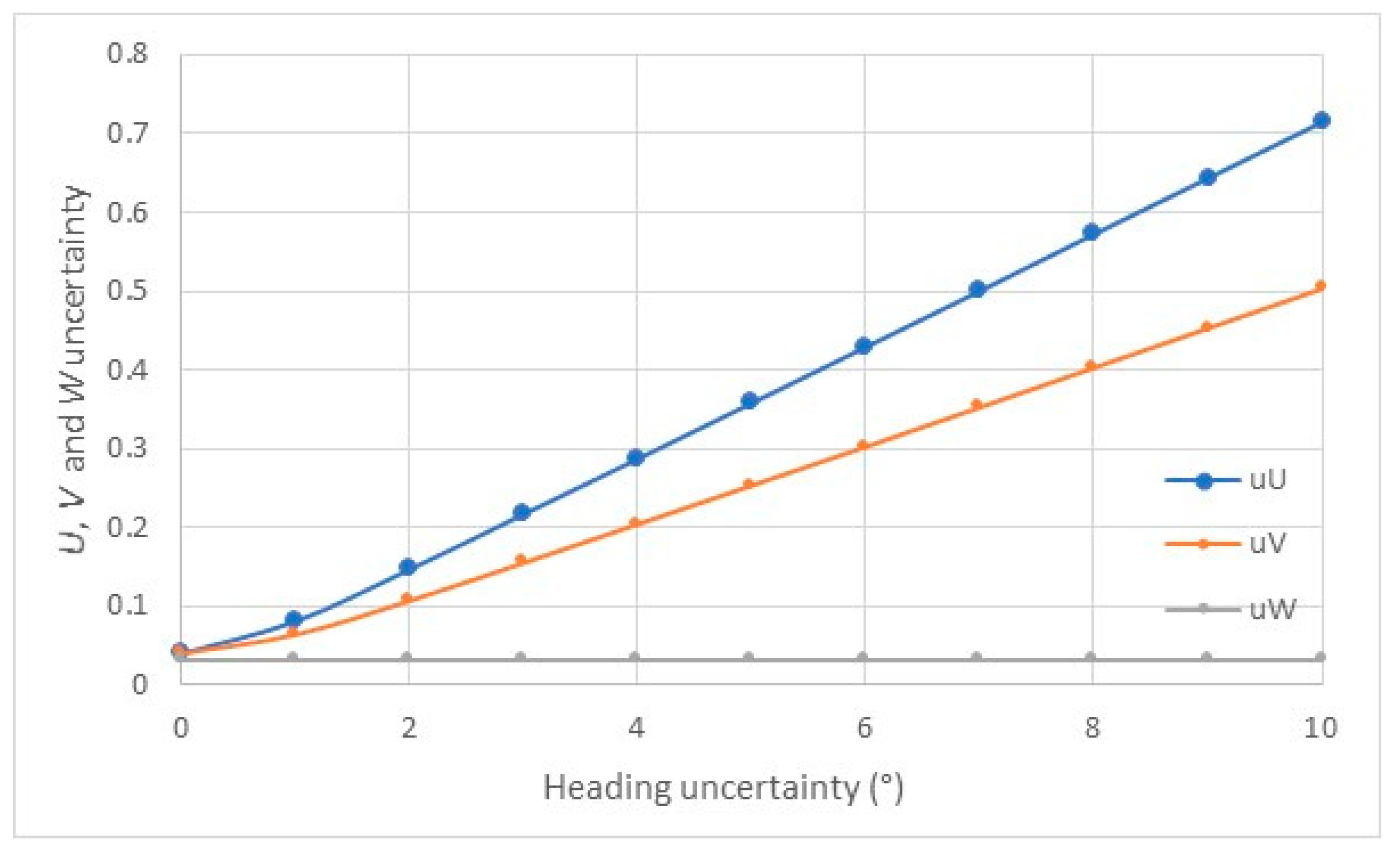
Figure 5.
Evolution of the uncertainties of U, V and W when the uncertainties on the tilt measurements increase of the same value from 0 to 4 °, for the values used in Table 1: α = 70 ° et θ = Ψ = 5 °, U = 2.87 m/s, V = - 4.09 m/s, W = - 0.85 m/s, uα= 0.59 °.
Figure 5.
Evolution of the uncertainties of U, V and W when the uncertainties on the tilt measurements increase of the same value from 0 to 4 °, for the values used in Table 1: α = 70 ° et θ = Ψ = 5 °, U = 2.87 m/s, V = - 4.09 m/s, W = - 0.85 m/s, uα= 0.59 °.
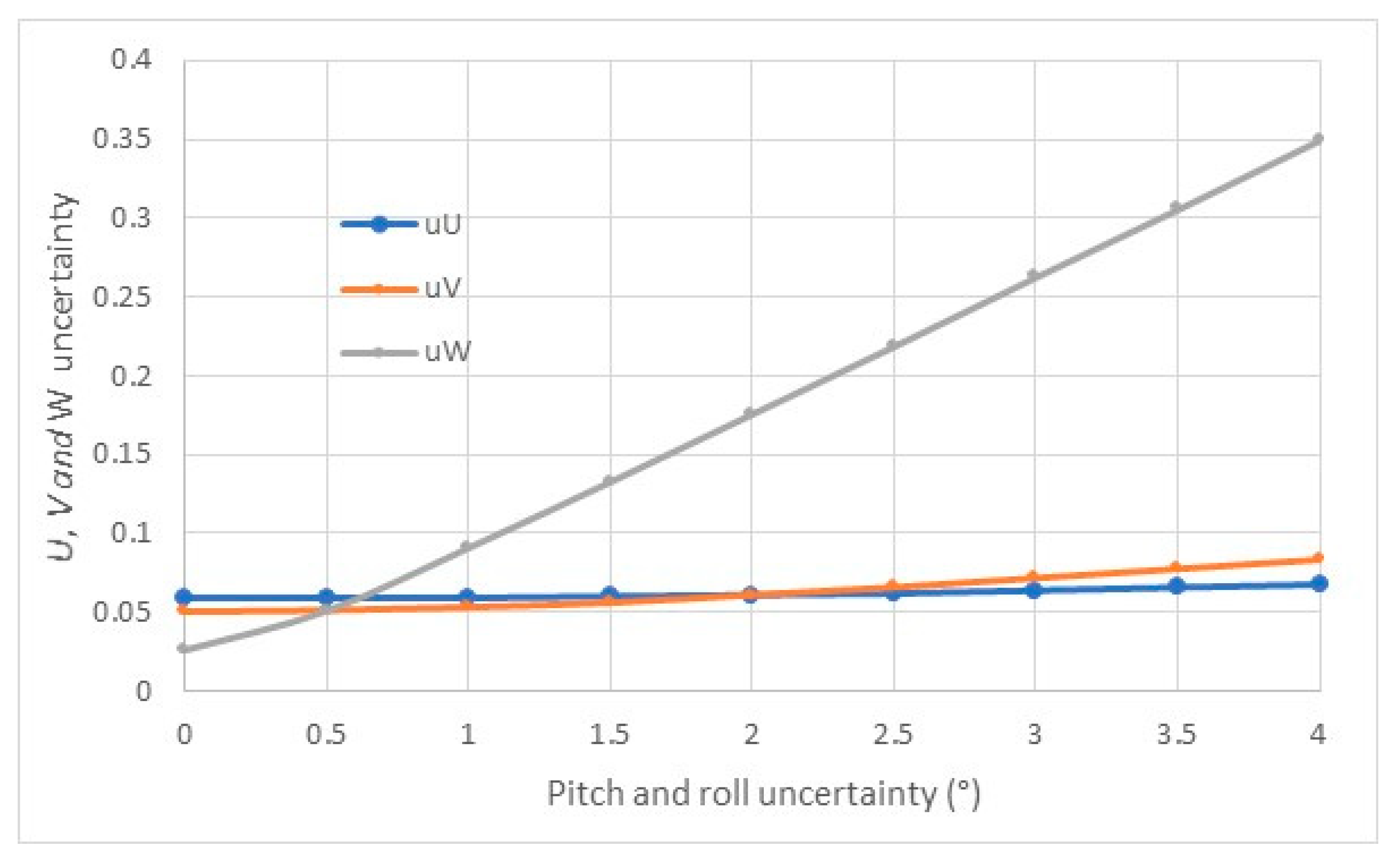
Figure 6.
(a) Evolution of the uncertainty on V1, V2 and V3 as a function of the uncertainty on the speed of sound. (b) Evolution of the uncertainty on U, V and W, as a function of the uncertainty on the speed of sound.
Figure 6.
(a) Evolution of the uncertainty on V1, V2 and V3 as a function of the uncertainty on the speed of sound. (b) Evolution of the uncertainty on U, V and W, as a function of the uncertainty on the speed of sound.
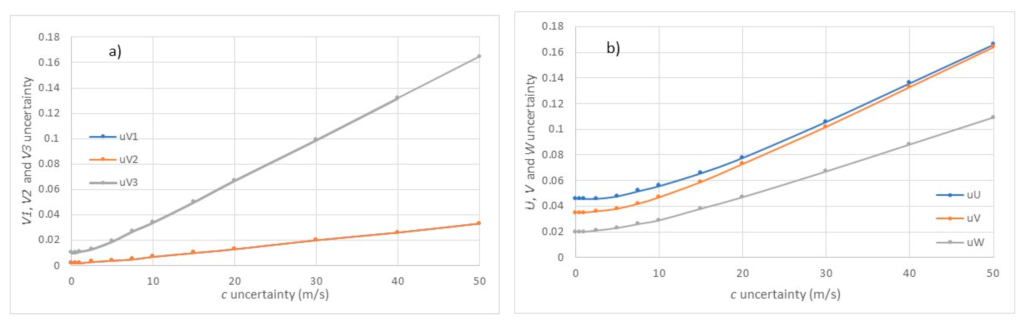

Table 1.
Sensitivity to the slant angle determination, obtained with current values of measured current.
Table 1.
Sensitivity to the slant angle determination, obtained with current values of measured current.
|
V1 |
-1 |
(m/s) |
β1 = 25 ° |
β2 = 25.1 ° |
β3 = 24.9 ° |
β1 - β2 |
β1 - β3 |
Sensitivity m/s/° |
|---|---|---|---|---|---|---|---|---|
| V2 | 1 | Vx | 4.732 | 4.715 | 4.750 | 0.0176 | -0.0178 | 0.18 |
| V3 | -5 | Vy | 1.183 | 1.179 | 1.188 | 0.0044 | -0.0044 | 0.04 |
| V4 | 5 | Vz | -1.379 | -1.380 | -1.378 | 0.0011 | -0.0011 | 0.01 |
Table 2.
Simulation of results that can be obtained with a Signature 500 kHz.
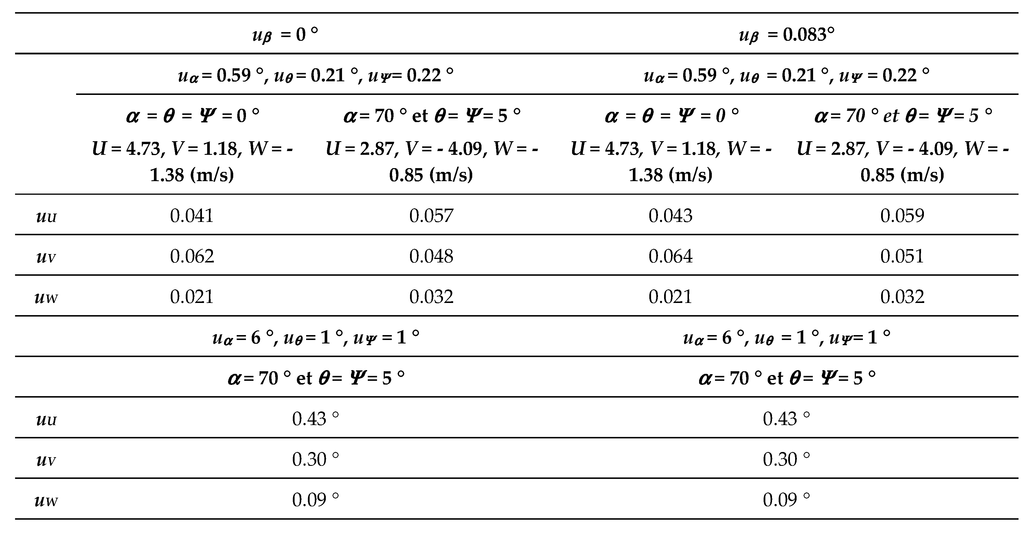 |
Table 3.
Simulation of results that can be obtained with a 600 kHz Workhorse Sentinel.
 |
Disclaimer/Publisher’s Note: The statements, opinions and data contained in all publications are solely those of the individual author(s) and contributor(s) and not of MDPI and/or the editor(s). MDPI and/or the editor(s) disclaim responsibility for any injury to people or property resulting from any ideas, methods, instructions or products referred to in the content. |
© 2025 by the authors. Licensee MDPI, Basel, Switzerland. This article is an open access article distributed under the terms and conditions of the Creative Commons Attribution (CC BY) license (http://creativecommons.org/licenses/by/4.0/).
Copyright: This open access article is published under a Creative Commons CC BY 4.0 license, which permit the free download, distribution, and reuse, provided that the author and preprint are cited in any reuse.


