
Submitted:
12 June 2025
Posted:
16 June 2025
You are already at the latest version
Abstract
This paper presents a modular hybrid mathematical model of bacterial fermentation developed by integrating a detailed kinetic model for the central carbon metabolism of E. coli with a simplified four-compartment model of a large stirred bioreactor. The model describes the growth dynamics of E. coli, taking into account the hydrodynamic characteristics of the cultivation environment and spatial concentration gradients. The first module simulates liquid exchange flows between neighboring reactor zones and tracks the spatial distribution of substrate, acetate, dissolved oxygen, and biomass, while the second one which is a kinetic model includes main metabolic pathways such as glycolysis, the tricarboxylic acid cycle, and oxidative phosphorylation. Numerical simulations reveal how mixing intensity affects concentration gradients and metabolic regimes across the reactor. Additionally, the model was used to identify an optimal mixing regime corresponding to the state where the system first enters the regime of complete aerobic substrate oxidation. The proposed model is applicable for numerical analysis of industrial-scale bioreactors and for predicting metabolic dynamics under various hydrodynamic conditions.
Keywords:
bioreactor
; mathematical model
; modular approach
; kinetic model
; compartment model
; systems biology
; BioUML
1. Introduction
The growing challenges of climate change demand effective and sustainable solutions to meet the needs of a rising global population while minimizing environmental impact [1]. Biomanufacturing is the biotechnological production of valuable chemicals [2] which has emerged as a key approach to address these challenges. By relying on renewable alternatives, biomanufacturing helps reduce dependence on fossil-based resources [2,3,4].
A continuous culturing is widely used in biomanufacturing, as it enables the controlled growth of microorganisms that produce target products. Advances in biological systems engineering have enabled laboratory-scale production of a wide range of compounds, including pharmaceuticals and precursors for materials and fuels, by utilizing microbial chassis at least in small amounts as a proof-of-concept [4,5,6,7,8,9]. There are also examples of biomanufacturing at an industrial scale, including the production of both high-value products (e.g., therapeutics, enzymes, antibiotics) and low-volume commodities (e.g., bioethanol, lactic acid, amino acids) [10]. However, the successful transition from a laboratory scale (with cultivation volumes ranging from milliliters to tens of liters) [11,12] to an industrial scale (with cultivation volumes reaching hundreds of cubic meters) [13,14] remains challenging and is often associated with significant physical, chemical, and biological limitations [2,12,15]. These constraints often prevent promising developments from being successfully translated into large-scale production [16,17].
One of the key limiting factors during scale-up is the emergence of spatial heterogeneity within large bioreactors. In laboratory-scale bioreactors, rapid mixing (on the order of seconds) results in a well-mixed, homogeneous environment. In contrast, industrial-scale bioreactors may require several minutes to reach ideal mixing conditions that lead to the formation of zones with concentration gradients of substrate, oxygen, and metabolic products [18,19]. For example, cells may shift toward anaerobic metabolism in zones with limited oxygen availability, leading to the accumulation of acetate – a byproduct that can inhibit microbial growth [20,21]. On the other hand, in substrate-depleted zones, cultures experience nutrient starvation, which reduces overall bioprocess efficiency [21,22].
Mathematical modeling plays a key role in analysis and optimization of industrial bioprocesses, as well as in mitigation of risks during scale-up from laboratory to industrial scale. Four main types of bioreactor models are commonly distinguished: kinetic, compartment, computational fluid dynamics (CFD), and hybrid models. Kinetic models provide a detailed description of metabolic pathways based on chemical kinetics, while generally neglecting hydrodynamic properties of the reactor [23]. In contrast, compartment and CFD models simplify the metabolic representation and instead focus on predicting the formation of mixing gradients. Compartment models consider the reactor as multiple ideally mixed zones (compartments), simulate liquid exchange flows between adjacent zones, and capture concentration gradients of substrate, oxygen, and other key compounds [19,24,25,26]. CFD models, on the other hand, calculate fluid dynamics by solving the Navier–Stokes equations, treating the liquid phase as a continuous medium [27,28]. While CFD models provide high spatial resolution, they require significant computational resources, making compartment models a computationally inexpensive alternative when moderate detail is sufficient. Finally, hybrid models combine kinetic models with either compartment or CFD models, in order to predict the spatial distribution of compound concentrations under realistic hydrodynamic conditions [29].
The objective of this study was to develop a hybrid mathematical model of an industrial bioreactor that simulates the growth of E. coli while accounting for key processes in central carbon metabolism and the spatial environment heterogeneity induced by mixing. To this end, we reproduced results from two previously published models on the BioUML platform: a simplified four-compartment model of a large stirred bioreactor [30] and a detailed kinetic model for the central carbon metabolism of E. coli [31]. These models were then combined into a unified modular model.
The structure of the paper is as follows. Section 2 provides a brief overview of the BioUML platform used for the model development and numerical simulations. In Section 3, the modular structure and main equations of the model are detailed. Section 4 presents the simulation results and their interpretation. Section 5 discusses the biological relevance of the results and outlines potential directions for further model refinement. Supplementary Materials (Tables S1–S3) provide the complete description of model equations, parameter values, and initial conditions.
2. Methods
2.1. Modeling Software
Model construction and numerical simulations were carried out using BioUML (Biological Universal Modeling Language, https://sirius-web.org/bioumlweb/), an open-source platform under active development [32,33]. BioUML is a Java-based software environment designed for modeling complex biological systems and analyzing biomedical data. It provides tools for visual representation of modeled biological systems and supports a wide range of systems biology standards, including Systems Biology Markup Language (SBML) [34] and Systems Biology Graphical Notation (SBGN) [35].
Model development in BioUML begins with representation of the modeled system as a compartmentalised graph. Based on this graph, the platform automatically generates Java code that defines the corresponding system of differential equations. Then this code is compiled and executed using internal numerical solvers to simulate the system’s dynamics.
To simplify the construction of models for complex systems, BioUML supports a modular approach, which enhances visual clarity and reduces the risk of technical errors. This approach, previously used to build various mathematical models [36,37], allows decomposition of any complex system into elementary components called modules (or submodels/blocks). Each module is defined independently and can follow its own formalism and level of abstraction. Interactions between modules are defined through variable connections, which, in the context of the bioreactor model, represent processes such as fluid exchange between adjacent compartments.
2.2. Model Parameters
2.3. Numerical Simulations
The unit of model time corresponds to one hour of real time. Numerical simulations were performed using the CVODE solver [38], ported to Java and integrated into the BioUML platform. All simulations presented in this paper were conducted for a duration of up to 1 hour.
3. Modular Model
3.1. Bioreactor Compartmentalization
The bioreactor compartment model utilizes the geometry of a 90-cubic-meter stirred bioreactor with four Rushton turbines, as described in [14,39]. The total reactor volume is divided into four vertical compartments using three horizontal planes, positioned equidistantly between the turbines. Three of the lower compartments have a volume of 20 m³ each, while the top compartment has a volume of 30 m³. A schematic representation of the bioreactor compartmentalization is shown in Figure 1.
3.2. Modular Model Structure
The mathematical model of a large stirred bioreactor, which describes the growth of E. coli and accounts for key processes in its central carbon metabolism as well as concentration gradients induced by mixing, was developed based on the principles of modular modeling for complex biological systems using the BioUML platform (see Section 2.1).
The BioUML implementation of the model consists of 9 modules: 4 metabolic modules (Metabolic_i) that calculate the dynamics of E. coli metabolism in the corresponding reactor zones; 4 compartment modules (Compartment_i) that calculate the liquid exchange flows between neighboring zones; and an auxiliary module (Feed_rate) that calculates the glucose feed rate to the top zone. The modular structure of the model in BioUML is shown in Figure 2.
The model includes 166 variables, 57 differential equations, 377 parameters, and 96 assignment operations. Hereafter, it is referred to as the modular model of the bioreactor.
3.3. Main Equations of the Modular Model
This section provides a brief overview of the main equations underlying the modular model of the bioreactor (Equations (1) – (23)). A complete description of all equations, parameter values, and initial conditions is given in Supplementary Materials (Tables S1 – S3).
The metabolic modules are based on a previously published kinetic model of the central carbon metabolism of E. coli [31]. This model includes the glycolytic pathway, tricarboxylic acid cycle, pentose phosphate pathway, Entner-Doudoroff pathway, anaplerotic pathway, glyoxylate shunt, oxidative phosphorylation, phosphotransferase and non- phosphotransferase systems, and alternative metabolic pathways. Regulation of metabolic activity is also incorporated through four key transcription factors: the cAMP receptor protein, the catabolite repressor/activator, the pyruvate dehydrogenase complex repressor, and the isocitrate lyase regulator.
The dynamics of each metabolic module are governed by the following set of equations (Equations (1) – (4)):
where denotes the biomass concentration in the compartment; is the vector of time-dependent intracellular variables (e.g., concentrations of metabolites, proteins and enzymes); is the vector of auxiliary variables, including intracellular regulatory proteins (such as transcription factors and their complexes with metabolites); is the vector of extracellular concentrations of glucose and acetate; the vector contains the concentrations of glucose and acetate in the feeding medium; is the vector of the kinetic parameters of the model; and is the dilution rate. The function defines the specific growth rate; corresponds to the specific uptake rates of glucose and acetate; and represents the system of intracellular mass balance equations.
To incorporate mixing dynamics, the system was extended with compartment modules based on the simplified compartment model of a bioreactor [31]. The total reactor volume was divided into four compartments (see Section 3.1). To simulate the mixing process, additional exchange terms were introduced into the right-hand side of the differential equations describing the extracellular concentrations of glucose, acetate, and biomass in the metabolic modules (Equations (5) – (7)):
where , and correspond to the extracellular concentrations of glucose, acetate, and biomass, respectively, and represents the liquid exchange flow between neighboring compartments i and j.
The calculation of liquid exchange between compartments was based on the volumetric pumping capacity of Rushton turbines under aerated conditions. It was assumed that half of the liquid flow generated by a turbine is directed downwards and the other half upwards [40,41]. Thus, the liquid exchange flow between compartments i and j () was defined as the average of the two volumetric flows meeting at the interface between these compartments (Equation (8)):
with the following expressions (Equations (9) – (15)) used to compute intermediate parameters:
where is the volumetric pumping capacity of a single Rushton turbine (with a power number ) in compartment i under aeration; is the ratio of aerated to unaerated power input; and are the Reynolds and Froude numbers, respectively; and are the impeller diameter and rotation speed; is the reactor diameter; is the liquid density; is the dynamic viscosity; is the gravitational acceleration; and denote the volumetric and mass flow rates of the gas, respectively; is the gas density; is the molecular weight of air; is the absolute pressure; is the universal gas constant; is the absolute temperature; is the height of the liquid above the impeller; is the excess pressure in the headspace of the reactor; and is the atmospheric pressure.
The original kinetic model of E. coli central metabolism [31] did not account for changes in oxygen concentration. Therefore, in the modular model of the bioreactor developed in this study, oxygen dynamics were incorporated by adapting the gas–liquid mass transfer equations from the compartment model of the bioreactor [30].
The gas hold-up (i.e., the volume fraction of the gas relative to the total volume) in each compartment was calculated using the following expressions (Equations (16) – (18)):
where represents the volume fraction of the bulk liquid; is the compartment volume; is the power input by a single impeller under aeration; and is the superficial gas velocity. Due to the gas hold-up, the total liquid volume across all compartments is slightly reduced compared to the full bioreactor volume of 90 m³.
Oxygen transfer from the gas phase to the bulk liquid in each compartment was modeled under the assumption that air bubbles do not coalesce. The following expressions (Equations (19) – (21)) were used:
where is the oxygen transfer rate; is the oxygen mass transfer coefficient; is the extracellular oxygen concentration; is the oxygen saturation concentration; is the bulk liquid volume; and is the mole fraction of oxygen in the gas phase.
The following expressions (Equations (22),(23)) were incorporated into the metabolic modules to compute the extracellular oxygen concentration:
where is the gas flow rate and is the number of moles of gas in the compartment.
The resulting extracellular oxygen concentration is consumed by the cells and subsequently utilized in oxidative phosphorylation, with the corresponding reaction rate contributing to the calculation of the specific growth rate. It is worth to note that the original metabolic model considers adaptation to oxygen availability according to an assumption of the oxygen excess in the medium, which allows for the instantaneous recovery of ATP, while the rate of ATP consumption is used in the rate of biomass production (Equations (24) – (28)):
where is the biomass concentration; is the specific growth rate; is the total ATP production flux; is the adjustable constant; and are the specific ATP production fluxes through oxidative phosphorylation; and indicate the phosphate/oxygen ratios for NADH and FADH2, respectively under aerobic conditions; and , , , , , , , , , , , , , are reaction rates for glucokinase, phosphofructokinase, glyceraldehyde 3-phosphate dehydrogenase, pyruvate kinase I, phosphoenolpyruvate synthase, acetate kinase, acetyl coenzyme A synthetase, α-keto-D-gluconate dehydrogenase, phosphoenolpyruvate carboxykinase, isocitrate dehydrogenase phosphatase/kinase, adenylate cyclase, pyruvate dehydrogenase, malate dehydrogenase, succinate dehydrogenase, respectively.
While in the proposed model, ATP is restored depending on the accumulated NADH and FADH2 and available oxygen (Equations (29) – (30)):
where , and are concentrations of NADH, FADH2 and intracellular oxygen, respectively; is the maximum oxidative phosphorylation rate; and are Michaelis–Menten constants.
Nevertheless, the process of oxidative phosphorylation is presented in a simplified form, taking into account the production of NADH, FADH2 and ATP. The absence of a complete oxidative phosphorylation process can become critical, especially in conditions of changing oxygen concentrations in the compartments of the bioreactor. This constraint is a jumping-off point of further development of the metabolic part of the modular model.
4. Results
4.1. Preliminary Information
The results of the numerical simulations for the modular model of the bioreactor are presented for a total simulation time of 1 hour, which was sufficient for the system to reach a steady state. It should be noted that reaching the stationary growth phase in bacterial cultures typically requires a longer timescale (5–10 hours) [43–47]. This highlights the need for further investigation of the factors and conditions influencing the long-term bioprocess dynamics, which will be addressed in future developments of the presented modular model.
Two different bioreactor mixing regimes were used: one corresponded to low mixing intensity (also referred to as “low settings”) with parameter values rpm, kg/s, bar; and another corresponded to high mixing intensity (“high settings”) with rpm, kg/s, bar. Additional simulations were performed by varying the mixing parameters between these two boundaries in order to identify an optimal mixing regime.
In all simulations, the specific glucose feed rate was set to 0.08 grams of substrate per gram of biomass per hour (gS/gX/h).
4.2. Simulation Results for the Boundary Mixing Regimes
Figure 3 shows the dynamics of extracellular metabolite concentrations and biomass across different compartments of the bioreactor under low and high mixing intensities.
At low mixing intensity (Figure 3, left column), oxygen depletion occurs in the upper compartments of the reactor because the upward transport of oxygen from the bottom zones is insufficient to sustain active metabolism. In contrast, under high mixing intensity (Figure 3, right column), the oxygen concentration remains sufficiently high throughout all compartments, thereby preventing acetate accumulation. Since glucose feeding occurs only in the top compartment, substrate depletion is observed in the lower zones. However, under high mixing intensity, glucose distribution becomes slightly more uniform across compartments, and, combined with high oxygen availability, this leads to an accelerated biomass growth rate.
The obtained results qualitatively agree with experimental observations reported in the published data regarding the influence of hydrodynamic conditions on substrate distribution, oxygen availability, and by-product formation in industrial-scale bioreactors [30].
E. coli can simultaneously assimilate substrates through both aerobic and anaerobic pathways. Under oxygen-limited conditions, the proportion of anaerobic metabolism varies, leading to the development of distinct metabolic regimes depending on the ratio between anaerobic and total substrate uptake rates.
Table 1 and Table 2 summarize the simulated substrate uptake rates and the corresponding metabolic regimes under different mixing conditions. The classification criteria for metabolic regimes were adopted from the original compartment model [30]: substrate starvation was defined by a total substrate uptake rate below 0.04 gS/gX/h; oxygen limitation was defined when the anaerobic substrate uptake rate exceeded 0.00001 gS/gX/h; in all other cases, substrate limitation was assumed.
Three metabolic regimes were identified from the simulations: oxygen limitation, substrate limitation, and substrate starvation. Under oxygen limitation, the oxygen transfer rate into the liquid phase is insufficient to fully oxidize the available substrate, forcing cells to partially shift to anaerobic metabolism. Substrate starvation occurs when the substrate uptake rate is too low to sustain cell growth, while metabolism remains fully aerobic. In the substrate limitation regime, growth is constrained by the availability of substrate, and all consumed substrate is completely oxidized without switching to anaerobic pathways.
It can be seen that adjusting the mixing parameters primarily influences whether glucose is consumed aerobically or anaerobically in the upper part of the reactor, while the lower compartments still experience significant substrate depletion. Interestingly, increasing the mixing intensity did not reduce the overall extent of substrate starvation across the reactor. This observation is consistent with the well-known fact that Rushton turbines promote efficient radial mixing but do not contribute to better axial (vertical) mixing [19,42]. As a result, glucose remains unevenly distributed along the height of the reactor, and enhanced mixing primarily improves oxygen transfer rather than homogenizing substrate concentrations.
4.3. Optimal Mixing Regime Identification
In addition to the two boundary regimes (with low and high mixing intensity), a series of simulations was conducted by varying three mixing-related parameters within the range defined by their respective boundary values using linear interpolation:
where is the new value of the interpolated parameter; and are its values under low and high mixing settings, respectively; and is the interpolation coefficient. A value of corresponds to the low settings, while corresponds to the high settings.
The aim of this analysis was to determine the minimum value of at which the steady-state acetate concentration in all compartments stabilizes at zero. This state was interpreted as an optimal mixing regime, in which anaerobic metabolism is fully suppressed at a lower mixing intensity than in the high settings scenario. This regime avoids excessive energy consumption stirring while maintaining optimal conditions for biomass growth.
For each value of with a step size of 0.01, a numerical simulation was performed, and the maximum acetate concentration across all compartments was recorded at the final simulation time point. Additionally, it was verified that the system had reached steady state. The resulting dependency is shown in Figure 4. The dynamics of extracellular metabolite and biomass concentrations for the identified optimal mixing regime are shown in Figure 5.
The acetate concentration was found to reach zero for the first time at , which corresponds to a mixing regime with the following parameter values: rpm, kg/s, bar.
Thus, the simulation results identified a minimum combination of mixing-related parameters at which acetate accumulation was suppressed in all compartments. This transition to fully aerobic substrate oxidation represents an optimal operating regime that sustains biomass growth rates comparable to those under high mixing conditions, while requiring lower energy demands for mixing.
5. Discussion
Fermentation processes in industrial-scale bioreactors are the focus of extensive experimental and computational research [18,48,49,50]. In this study, we developed a modular mathematical model of an industrial-scale stirred bioreactor capable of simulating the dynamics of metabolic processes in E. coli within different bioreactor zones, while explicitly accounting for concentration gradients induced by mixing. The main advantage of the model lies in its integration of a detailed kinetic description of the central carbon metabolism with a simplified hydrodynamic representation of the cultivation environment. This hybrid modeling approach provides an improved capability to capture how mixing conditions and spatial concentration gradients affect the metabolic responses of cell cultures.
The simulation results demonstrated that mixing intensity has a substantial impact on the overall dynamics within the reactor. Under low mixing intensity, oxygen limitation was observed in the upper reactor compartments, forcing cells to partially switch to anaerobic metabolism and leading to acetate accumulation. In contrast, under high mixing intensity, both substrate and oxygen are more evenly distributed, preventing acetate formation and enhancing biomass growth. Additionally, computational analysis allowed identification of an optimal mixing regime, characterized by zero steady-state acetate concentration at more than 40% lower mixing intensity compared to the high-mixing scenario. This result highlights the model’s potential in identifying energy-efficient bioreactor operating conditions, which simultaneously improve oxygen availability for aerobic metabolism and reduce risks of mechanical stress on cells associated with excessively high mixing rates [51,52].
However, the current implementation of the modular model relies on a simplified four-compartment representation of hydrodynamics, which does not account for potential intra-compartmental gradients of substrate and oxygen concentrations. This simplification leads to artificially steep transitions between metabolic regimes. In realistic systems, it is reasonable to expect an intermediate region between zones of oxygen limitation and substrate starvation – where substrate is still available but no longer sufficient to meet the full metabolic demands of the cells. The existence of such transitional regions has been computationally confirmed using CFD-based models [30].
Therefore, future improvements of the presented model should focus on incorporating more refined spatial concentration distributions, either by increasing the complexity of compartmentalization or by integrating CFD approaches.
6. Conclusions
In this study, we developed a modular mathematical model of an industrial-scale stirred bioreactor, integrating key aspects of E. coli metabolism with hydrodynamic properties of the cultivation environment. The model combines a simplified four-compartment model of a large stirred bioreactor with a detailed kinetic model for the central carbon metabolism of E. coli.
The compartment model divides the reactor volume into distinct zones and calculates local concentrations of glucose, oxygen, acetate, and biomass, as well as liquid exchange flows between adjacent compartments. The kinetic model incorporates detailed metabolic pathways, including glycolysis, the tricarboxylic acid cycle, oxidative phosphorylation, and accounts for shifts between aerobic and anaerobic metabolism based on oxygen availability. Compared to existing hybrid models that combine metabolic kinetics with hydrodynamic effects, the presented model provides the most detailed kinetic component, enabling more accurate simulation of metabolic pathways.
Numerical simulation results demonstrated the substantial impact of mixing parameters on spatial distributions of compounds and corresponding metabolic regimes within the bioreactor. Additionally, computational analysis identified an optimal mixing regime that eliminates anaerobic metabolism while reducing energy consumption for stirring. The developed model provides a computational tool for simulating cultivation processes in industrial bioreactors and analyzing metabolic dynamics under various hydrodynamic conditions.
Supplementary Materials
The following supporting information can be downloaded at the website of this paper posted on Preprints.org, Table S1: Model Reactions; Table S2: Model Variables; Table S3: Model Parameters; File S1: Mathematical Model (.omex).
Author Contributions
Conceptualization, P.Yu.K., I.R.A. and F.A.K.; methodology, P.Yu.K., I.R.A. and F.A.K.; software, F.A.K.; validation, P.Yu.K., V.A.K. and I.R.A.; formal analysis, P.Yu.K. and V.A.K.; investigation, P.Yu.K.; writing—original draft preparation, P.Yu.K. and V.A.K.; writing—review and editing, P.Yu.K., V.A.K., I.R.A. and F.A.K.; visualization, P.Yu.K.; supervision, F.A.K.; funding acquisition, F.A.K. All authors have read and agreed to the published version of the manuscript.
Funding
This work was supported by the grant of the state program of the «Sirius» Federal Territory «Scientific and technological development of the «Sirius» Federal Territory» (Agreement №18-03 date 10.09.2024).
Institutional Review Board Statement
Not applicable.
Informed Consent Statement
Not applicable.
Data Availability Statement
The implementation of the model is available in the web version of the BioUML platform and is stored in the GitLab repository at: https://gitlab.sirius-web.org/bioreactor/modular-model-of-bioreactor.
Conflicts of Interest
The authors declare no conflict of interest. The funders had no role in the design of the study; in the collection, analyses, or interpretation of data; in the writing of the manuscript; or in the decision to publish the results.
References
- Calvin, K.; Dasgupta, D.; Krinner, G.; Mukherji, A.; Thorne, P.W.; Trisos, C.; Romero, J.; Aldunce, P.; Barrett, K.; Blanco, G.; et al. Climate change 2023: Synthesis report. Contribution of Working Groups I, II and III to the Sixth Assessment Report of the Intergovernmental Panel on Climate Change; Lee, H., Romero, J., Eds.; Intergovernmental Panel on Climate Change (IPCC): Geneva, Switzerland, 2023. [Google Scholar] [CrossRef]
- Cordell, W.T.; Avolio, G.; Takors, R.; Pfleger, B.F. Milligrams to kilograms: Making microbes work at scale. Trends in Biotechnology 2023, 41, 1442–1457. [Google Scholar] [CrossRef]
- Noorman, H.J.; Heijnen, J.J. Biochemical engineering’s grand adventure. Chemical Engineering Science 2017, 170, 677–693. [Google Scholar] [CrossRef]
- Straathof, A.J.J.; Wahl, S.A.; Benjamin, K.R.; Takors, R.; Wierckx, N.; Noorman, H.J. Grand research challenges for sustainable industrial biotechnology. Trends in Biotechnology 2019, 37, 1042–1050. [Google Scholar] [CrossRef] [PubMed]
- Keasling, J.D. Manufacturing molecules through metabolic engineering. Science 2010, 330, 1355–1358. [Google Scholar] [CrossRef] [PubMed]
- Stephanopoulos, G. Synthetic biology and metabolic engineering. ACS Synthetic Biology 2012, 1, 514–525. [Google Scholar] [CrossRef]
- Casini, A.; Chang, F.-Y.; Eluere, R.; King, A.M.; Young, E.M.; Dudley, Q.M.; Karim, A.; Pratt, K.; Bristol, C.; Forget, A.; et al. A pressure test to make 10 molecules in 90 days: External evaluation of methods to engineer biology. Journal of the American Chemical Society 2018, 140, 4302–4316. [Google Scholar] [CrossRef]
- Lee, S.Y.; Kim, H.U.; Chae, T.U.; Cho, J.S.; Kim, J.W.; Shin, J.H.; Kim, D.I.; Ko, Y.-S.; Jang, W.D.; Jang, Y.-S. A comprehensive metabolic map for production of bio-based chemicals. Nature Catalysis 2019, 2, 18–33. [Google Scholar] [CrossRef]
- Voigt, C.A. Synthetic biology 2020–2030: Six commercially-available products that are changing our world. Nature Communications 2020, 11, 6369. [Google Scholar] [CrossRef] [PubMed]
- Jullesson, D.; David, F.; Pfleger, B.; Nielsen, J. Impact of synthetic biology and metabolic engineering on industrial production of fine chemicals. Biotechnology Advances 2015, 33, 1395–1402. [Google Scholar] [CrossRef]
- Hemmerich, J.; Noack, S.; Wiechert, W.; Oldiges, M. Microbioreactor systems for accelerated bioprocess development. Biotechnology Journal 2018, 13, 1700141. [Google Scholar] [CrossRef]
- Crater, J.S.; Lievense, J.C. Scale-up of industrial microbial processes. FEMS Microbiology Letters 2018, 365, fny138. [Google Scholar] [CrossRef]
- Noorman, H. An industrial perspective on bioreactor scale-down: What we can learn from combined large-scale bioprocess and model fluid studies. Biotechnology Journal 2011, 6, 934–943. [Google Scholar] [CrossRef]
- Nadal-Rey, G. Modelling of gradients in industrial aerobic fed-batch fermentation processes. Ph.D. Thesis, Technical University of Denmark, Denmark, 2020. https://backend.orbit.dtu.dk/ws/portalfiles/portal/244849808/201001_PhDThesis_GiselaNadalRey.pdf.
- Biggs, B.W.; Alper, H.S.; Pfleger, B.F.; Tyo, K.E.J.; Santos, C.N.S.; Ajikumar, P.K.; Stephanopoulos, G. Enabling commercial success of industrial biotechnology. Science 2021, 374, 1563–1565. [Google Scholar] [CrossRef]
- Kampers, L.F.C.; Asin-Garcia, E.; Schaap, P.J.; Wagemakers, A.; Martins dos Santos, V.A.P. From innovation to application: Bridging the valley of death in industrial biotechnology. Trends in Biotechnology 2021, 39, 1240–1242. [Google Scholar] [CrossRef]
- de Lorenzo, V.; Couto, J. The important versus the exciting: Reining contradictions in contemporary biotechnology. Microbial Biotechnology 2018, 12, 32–34. [Google Scholar] [CrossRef]
- Nadal-Rey, G.; McClure, D.D.; Kavanagh, J.M.; Cornelissen, S.; Fletcher, D.F.; Gernaey, K.V. Understanding gradients in industrial bioreactors. Biotechnology Advances 2021, 46, 107660. [Google Scholar] [CrossRef]
- Vrábel, P.; van der Lans, R.G.J.M.; Luyben, K.Ch.A.M.; Boon, L.; Nienow, A.W. Mixing in large-scale vessels stirred with multiple radial or radial and axial up-pumping impellers: Modelling and measurements. Chemical Engineering Science 2000, 55, 5881–5896. [Google Scholar] [CrossRef]
- Xu, B.; Jahic, M.; Enfors, S.-O. Modeling of overflow metabolism in batch and fed-batch cultures of Escherichia coli. Biotechnology Progress 1999, 15, 81–90. [Google Scholar] [CrossRef]
- Wolfe, A.J. The acetate switch. Microbiology and Molecular Biology Reviews 2005, 69, 12–50. [Google Scholar] [CrossRef]
- Neubauer, P.; Åhman, M.; Törnkvist, M.; Larsson, G.; Enfors, S.-O. Response of guanosine tetraphosphate to glucose fluctuations in fed-batch cultivations of Escherichia coli. Journal of Biotechnology 1995, 43, 195–204. [Google Scholar] [CrossRef]
- Almquist, J.; Cvijovic, M.; Hatzimanikatis, V.; Nielsen, J.; Jirstrand, M. Kinetic models in industrial biotechnology – Improving cell factory performance. Metabolic Engineering 2014, 24, 38–60. [Google Scholar] [CrossRef]
- Vrábel, P.; van der Lans, R.G.J.M.; Cui, Y.Q.; Luyben, K.Ch.A.M. Compartment model approach. Chemical Engineering Research and Design 1999, 77, 291–302. [Google Scholar] [CrossRef]
- Oosterhuis, N.M.G.; Kossen, N.W.F. Dissolved oxygen concentration profiles in a production-scale bioreactor. Biotechnology and Bioengineering 1984, 26, 546–550. [Google Scholar] [CrossRef]
- Reuss, M.; Bajpai, R. Stirred tank models. In Biotechnology; Wiley: 1991; pp. 299–348. [CrossRef]
- Spann, R.; Glibstrup, J.; Pellicer-Alborch, K.; Junne, S.; Neubauer, P.; Roca, C.; Kold, D.; Lantz, A.E.; Sin, G.; Gernaey, K.V.; Krühne, U. CFD predicted pH gradients in lactic acid bacteria cultivations. Biotechnology and Bioengineering 2018, 116, 769–780. [Google Scholar] [CrossRef]
- Kuschel, M.; Takors, R. Simulated oxygen and glucose gradients as a prerequisite for predicting industrial scale performance a priori. Biotechnology and Bioengineering 2020, 117, 2760–2770. [Google Scholar] [CrossRef]
- Spann, R.; Gernaey, K.V.; Sin, G. A compartment model for risk-based monitoring of lactic acid bacteria cultivations. Biochemical Engineering Journal 2019, 151, 107293. [Google Scholar] [CrossRef]
- Bafna-Rührer, J. Strategies and tools to select E. coli fermenterphiles for industrial application. Ph.D. Thesis, Technical University of Denmark, Denmark, 2024. https://orbit.dtu.dk/files/375573898/Submission_version_PhD_thesis_JBR.pdf.
- Jahan, N.; Maeda, K.; Matsuoka, Y.; Sugimoto, Y.; Kurata, H. Development of an accurate kinetic model for the central carbon metabolism of Escherichia coli. Microbial Cell Factories 2016, 15, 112. [Google Scholar] [CrossRef]
- Kolpakov, F.; Akberdin, I.; Kashapov, T.; Kiselev, I.; Kolmykov, S.; Kondrakhin, Y.; Kutumova, E.; Mandrik, N.; Pintus, S.; Ryabova, A.; et al. BioUML: An integrated environment for systems biology and collaborative analysis of biomedical data. Nucleic Acids Research 2019, 47, W225–W233. [Google Scholar] [CrossRef]
- Kolpakov, F.; Akberdin, I.; Kiselev, I.; Kolmykov, S.; Kondrakhin, Y.; Kulyashov, M.; Kutumova, E.; Pintus, S.; Ryabova, A.; Sharipov, R.; et al. BioUML—towards a universal research platform. Nucleic Acids Research 2022, 50, W124–W131. [Google Scholar] [CrossRef]
- Hucka, M.; Bergmann, F.T.; Chaouiya, C.; Dräger, A.; Hoops, S.; Keating, S.M.; König, M.; Novère, N.L.; Myers, C.J.; Olivier, B.G.; et al. The Systems Biology Markup Language (SBML): Language specification for Level 3 Version 2 Core Release 2. Journal of Integrative Bioinformatics 2019, 16, jib-2019-0021. [Google Scholar] [CrossRef] [PubMed]
- Novère, N.L.; Hucka, M.; Mi, H.; Moodie, S.; Schreiber, F.; Sorokin, A.; Demir, E.; Wegner, K.; Aladjem, M.I.; Wimalaratne, S.M.; et al. The Systems Biology Graphical Notation. Nature Biotechnology 2009, 27, 735–741. [Google Scholar] [CrossRef]
- Kutumova, E.O.; Akberdin, I.R.; Egorova, V.S.; Kolesova, E.P.; Parodi, A.; Pokrovsky, V.S.; Zamyatnin, A.A. Jr; Kolpakov, F.A. Physiologically based pharmacokinetic model for predicting the biodistribution of albumin nanoparticles after induction and recovery from acute lung injury. Heliyon 2024, 10, e30962. [Google Scholar] [CrossRef]
- Miroshnichenko, M.I.; Kolpakov, F.A.; Akberdin, I.R. A modular mathematical model of the immune response for investigating the pathogenesis of infectious diseases. Viruses 2025, 17, 589. [Google Scholar] [CrossRef]
- Hindmarsh, A.C.; Brown, P.N.; Grant, K.E.; Lee, S.L.; Serban, R.; Shumaker, D.E.; Woodward, C.S. SUNDIALS. ACM Transactions on Mathematical Software 2005, 31, 363–396. [Google Scholar] [CrossRef]
- Nadal-Rey, G.; McClure, D.D.; Kavanagh, J.M.; Cassells, B.; Cornelissen, S.; Fletcher, D.F.; Gernaey, K.V. Development of dynamic compartment models for industrial aerobic fed-batch fermentation processes. Chemical Engineering Journal 2021, 420, 130402. [Google Scholar] [CrossRef]
- Oosterhuis, N.M.G. Scale-up of bioreactors: A scale-down approach. Ph.D. Thesis, TU Delft, Netherlands, 1984. http://resolver.tudelft.nl/uuid:03a887b7-8c20-4052-8d6b-7fe76918d7ec.
- Noorman, H.J.; van Winden, W.; Heijnen, J.J.; van der Lans, R.G.J.M. Intensified fermentation processes and equipment. In Intensification of Biobased Processes; The Royal Society of Chemistry: 2018; pp. 1–41. [CrossRef]
- Lapin, A.; Müller, D.; Reuss, M. Dynamic behavior of microbial populations in stirred bioreactors simulated with Euler−Lagrange methods: Traveling along the lifelines of single cells. Industrial & Engineering Chemistry Research 2004, 43, 4647–4656. [Google Scholar] [CrossRef]
- Hewitt, C.J.; Boon, L.A.; McFarlane, C.M.; Nienow, A.W. The use of flow cytometry to study the impact of fluid mechanical stress on Escherichia coli W3110 during continuous cultivation in an agitated bioreactor. Biotechnology and Bioengineering 1998, 59, 612–620. [Google Scholar] [CrossRef]
- Guardia Alba, M.J.; García Calvo, E. Characterization of bioreaction processes: Aerobic Escherichia coli cultures. Journal of Biotechnology 2000, 84, 107–118. [Google Scholar] [CrossRef]
- Lapin, A.; Schmid, J.; Reuss, M. Modeling the dynamics of E. coli populations in the three-dimensional turbulent field of a stirred-tank bioreactor—A structured–segregated approach. Chemical Engineering Science 2006, 61, 4783–4797. [Google Scholar] [CrossRef]
- Glazyrina, J.; Materne, E.-M.; Dreher, T.; Storm, D.; Junne, S.; Adams, T.; Greller, G.; Neubauer, P. High cell density cultivation and recombinant protein production with Escherichia coli in a rocking-motion-type bioreactor. Microbial Cell Factories 2010, 9, 42. [Google Scholar] [CrossRef]
- Zambrano, J.; Carlsson, B.; Diehl, S. Optimal steady-state design of zone volumes of bioreactors with Monod growth kinetics. Biochemical Engineering Journal 2015, 100, 59–66. [Google Scholar] [CrossRef]
- Garcia-Ochoa, F.; Gomez, E. Bioreactor scale-up and oxygen transfer rate in microbial processes: An overview. Biotechnology Advances 2009, 27, 153–176. [Google Scholar] [CrossRef]
- Tarlak, F. The use of predictive microbiology for the prediction of the shelf life of food products. Foods 2023, 12, 4461. [Google Scholar] [CrossRef]
- de Mello, A.F.M.; de Souza Vandenberghe, L.P.; Herrmann, L.W.; Letti, L.A.J.; Burgos, W.J.M.; Scapini, T.; Manzoki, M.C.; de Oliveira, P.Z.; Soccol, C.R. Strategies and engineering aspects on the scale-up of bioreactors for different bioprocesses. Systems Microbiology and Biomanufacturing 2023, 4, 365–385. [Google Scholar] [CrossRef]
- de Lamotte, A.; Delafosse, A.; Calvo, S.; Delvigne, F.; Toye, D. Investigating the effects of hydrodynamics and mixing on mass transfer through the free-surface in stirred tank bioreactors. Chemical Engineering Science 2017, 172, 125–142. [Google Scholar] [CrossRef]
- Garcia-Ochoa, F.; Gomez, E.; Santos, V.E. Fluid dynamic conditions and oxygen availability effects on microbial cultures in STBR: An overview. Biochemical Engineering Journal 2020, 164, 107803. [Google Scholar] [CrossRef]
Figure 1.
Schematic representation of the bioreactor compartmentalization. Substrate is fed through the top of the reactor (). Bidirectional liquid exchange flows () occur between the compartments i and j. Air is supplied to the reactor from the bottom (air), with the molar airflow moving only upwards, and no back mixing of the gas phase is considered. Bioreactor geometry: reactor height H=10.464 m, reactor diameter T=3.476 m, distance between turbines L=2.32 m, distance from the bottom turbine to the reactor bottom L1=1.271 m, turbine diameter D=0.936 m.
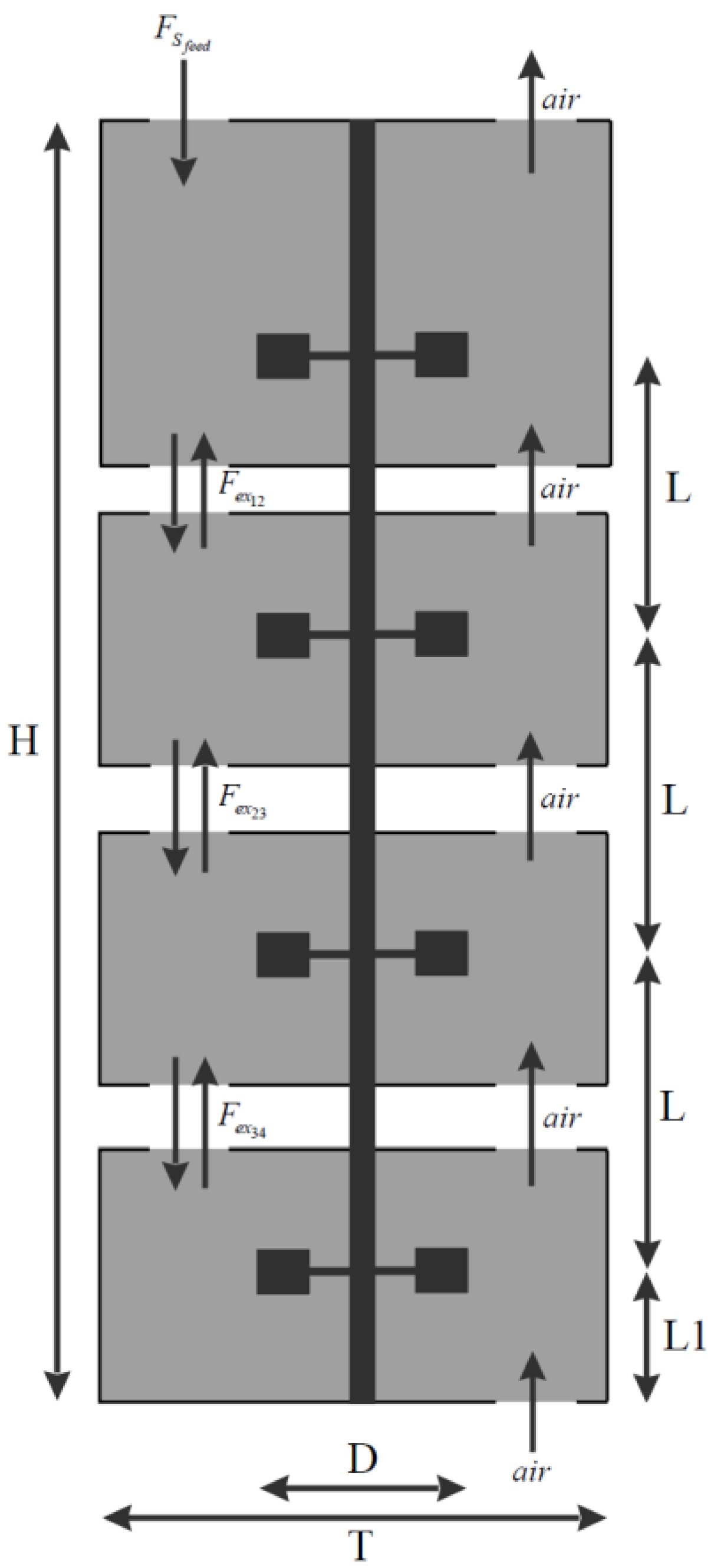
Figure 2.
Modular structure of the model. The parameters , and specify the stirrer speed, gas inflow rate, and excess pressure in the top part of the bioreactor, respectively, and together define the mixing intensity. Depending on the mixing regime, the compartment modules calculate the following hydrodynamic quantities: liquid exchange flow , liquid volume in the compartment excluding gas hold-up , oxygen mass transfer coefficient , absolute pressure , gas flow rate , and the number of moles of gas in the compartment . These quantities are transferred to the corresponding metabolic blocks, where they are considered in the calculation of metabolic activity. Neighboring metabolic compartments exchange fluxes of substances, including concentrations of substrate (glucose) , acetate , biomass , dissolved oxygen , and the mole fraction of oxygen in the gas phase .

Figure 3.
Numerical simulation results of the modular model of the bioreactor under low (left column) and high (right column) mixing intensity. The plots show concentrations of (A,B) glucose, (C,D) acetate, (E,F) dissolved oxygen, and (G,H) biomass in the cultivation medium. Colors indicate compartment identity: green – compartment 1 (top), blue – 2, orange – 3, red – 4 (bottom).
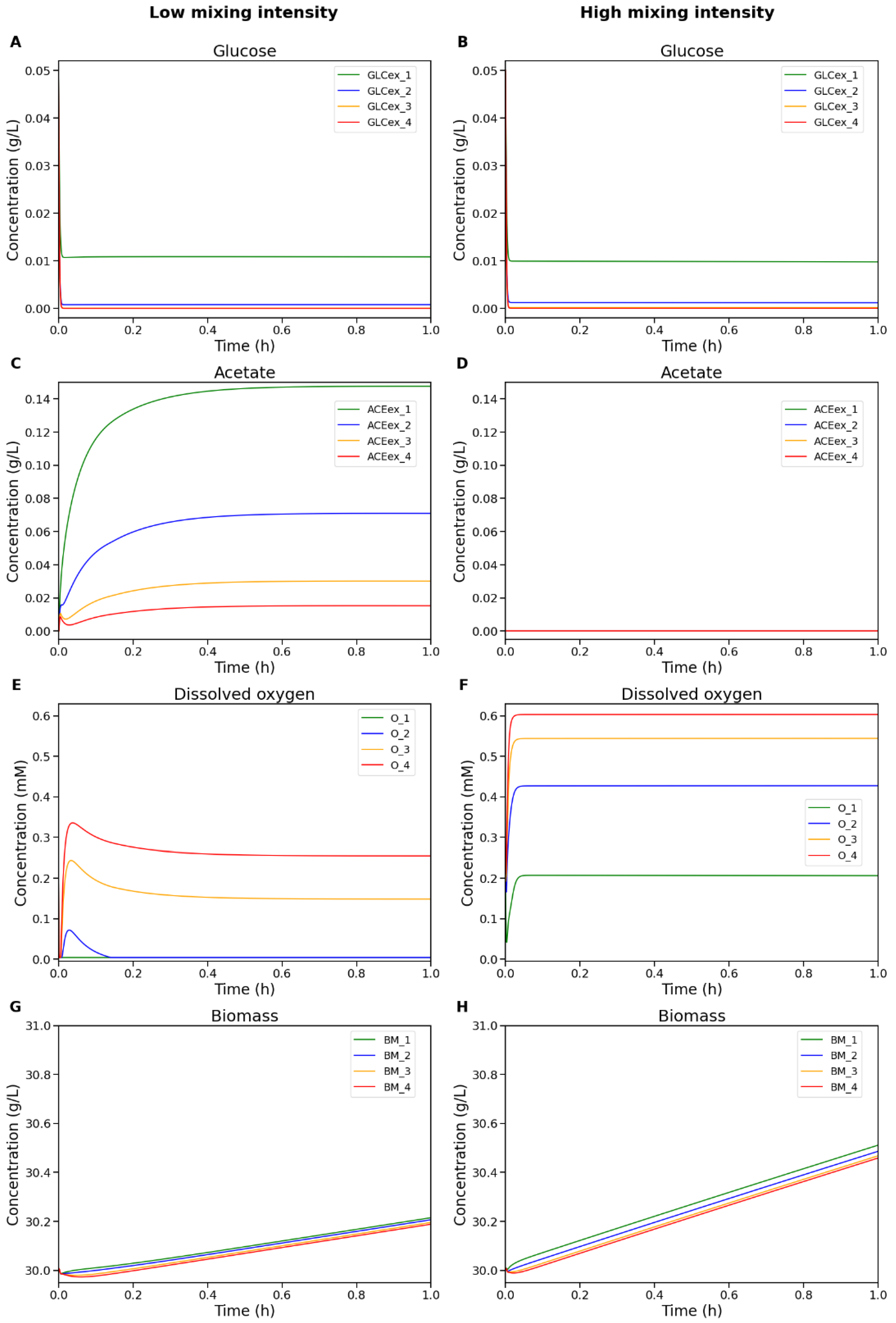
Figure 4.
Dependence of the maximum steady-state acetate concentration (ACEexMax) across all compartments on the interpolation parameter , which defines the mixing intensity.
Figure 4.
Dependence of the maximum steady-state acetate concentration (ACEexMax) across all compartments on the interpolation parameter , which defines the mixing intensity.
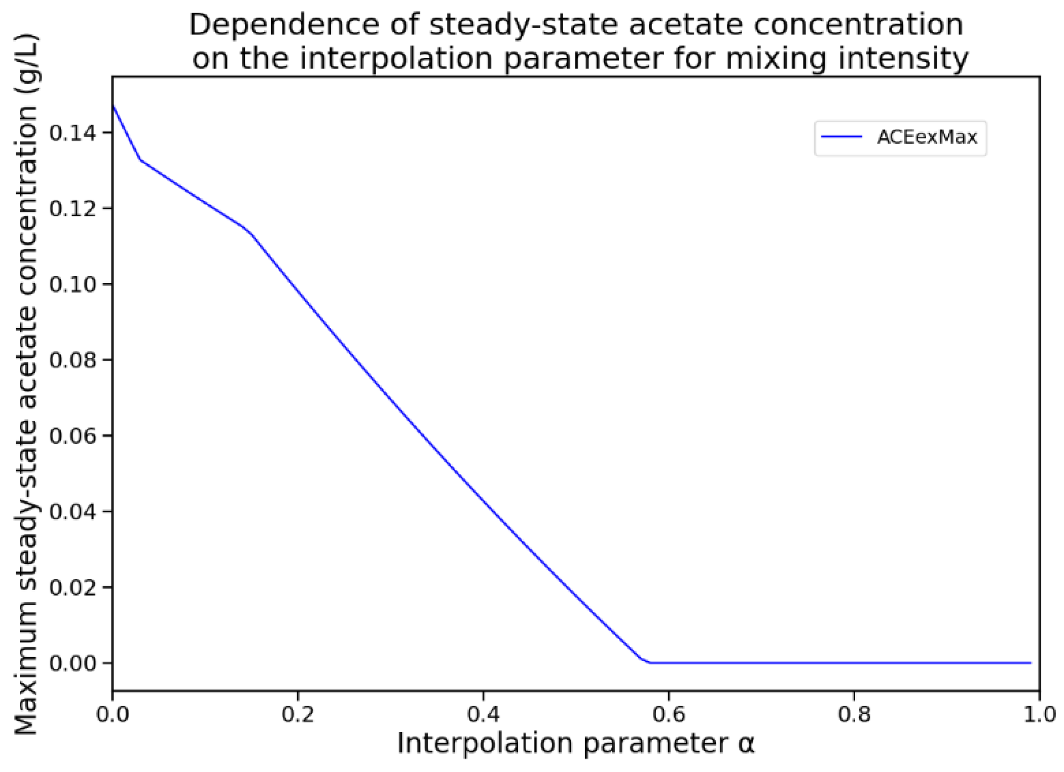
Figure 5.
Numerical simulation results of the modular model of the bioreactor under the optimal mixing regime. The plots show concentrations of (A) glucose, (B) acetate, (C) dissolved oxygen, and (D) biomass in the cultivation medium. Color coding for compartments is the same as in Figure 3.
Figure 5.
Numerical simulation results of the modular model of the bioreactor under the optimal mixing regime. The plots show concentrations of (A) glucose, (B) acetate, (C) dissolved oxygen, and (D) biomass in the cultivation medium. Color coding for compartments is the same as in Figure 3.
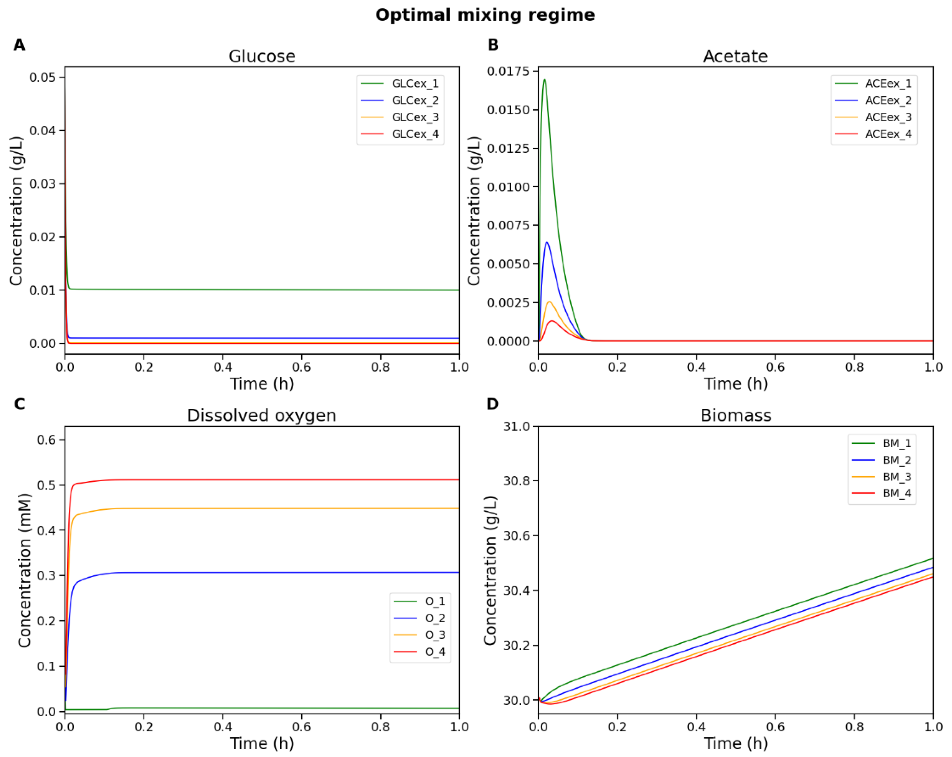

Table 1.
Simulated substrate uptake rates and corresponding metabolic regimes in bioreactor compartments under low mixing intensity.
Table 1.
Simulated substrate uptake rates and corresponding metabolic regimes in bioreactor compartments under low mixing intensity.
| Compartment | Total substrate uptake (gS/gX/h) |
Anaerobic substrate uptake (gS/gX/h) |
Metabolic regime |
|---|---|---|---|
| 1 (top) | 0.2245 | 0.1984 | Oxygen limitation |
| 2 | 0.0196 | 0.0 | Substrate starvation |
| 3 | 0.0015 | 0.0 | Substrate starvation |
| 4 (bottom) | 1.2522 × 10⁻⁴ | 0.0 | Substrate starvation |
Table 2.
Simulated substrate uptake rates and corresponding metabolic regimes in bioreactor compartments under high mixing intensity.
Table 2.
Simulated substrate uptake rates and corresponding metabolic regimes in bioreactor compartments under high mixing intensity.
| Compartment | Total substrate uptake (gS/gX/h) |
Anaerobic substrate uptake (gS/gX/h) |
Metabolic regime |
|---|---|---|---|
| 1 (top) | 0.2123 | 0.0 | Substrate limitation |
| 2 | 0.0304 | 0.0 | Substrate starvation |
| 3 | 0.0038 | 0.0 | Substrate starvation |
| 4 (bottom) | 5.4551 × 10⁻⁴ | 0.0 | Substrate starvation |
Disclaimer/Publisher’s Note: The statements, opinions and data contained in all publications are solely those of the individual author(s) and contributor(s) and not of MDPI and/or the editor(s). MDPI and/or the editor(s) disclaim responsibility for any injury to people or property resulting from any ideas, methods, instructions or products referred to in the content. |
© 2025 by the authors. Licensee MDPI, Basel, Switzerland. This article is an open access article distributed under the terms and conditions of the Creative Commons Attribution (CC BY) license (http://creativecommons.org/licenses/by/4.0/).
Copyright: This open access article is published under a Creative Commons CC BY 4.0 license, which permit the free download, distribution, and reuse, provided that the author and preprint are cited in any reuse.


