
Submitted:
13 June 2025
Posted:
17 June 2025
You are already at the latest version
Abstract
Climate concerns are driving the automotive industry to adopt advanced manufacturing technologies that aim to improve energy efficiency and reduce vehicle weight. In this context, lightweight structural materials such as aluminum alloys have gained significant attention due to their favorable strength-to-weight ratio. Laser welding plays a crucial role in assembling such materials, offering high flexibility and fast joining capabilities for thin aluminum sheets. However, welding these materials presents specific challenges, particularly in controlling heat input to minimize distortions and ensure consistent weld quality. As a result, numerical simulations based on the Finite Element Method (FEM) are essential for predicting weld-induced phenomena and optimizing process performance. This study investigates welding-induced distortions in laser butt welding of 1.5 mm-thick Al 6061 samples through FEM simulations performed in the ESI Sysweld environment. The methodology provided by the software is based on the Moving Heat Source (MHS) model, which simulates the physical movement of the heat source and typically requires extensive calibration through destructive metallographic testing. This transient approach enables the detailed prediction of thermal, metallurgical, and mechanical behavior, but it is computationally demanding. To improve efficiency, the Imposed Thermal Cycle (ITC) model is often used. In this technique, a thermal cycle, extracted from an MHS simulation or experimental data, is imposed on predefined subregions of the model, allowing only mechanical behavior to be simulated while reducing computation time. To avoid MHS-based calibration, this work proposes using thermal cycles acquired in-line during welding via infrared thermography as direct input for the ITC model. The method was validated experimentally and numerically, showing good agreement in the prediction of distortions and a significant reduction in workflow time. The integration of real process data into the simulation enables a virtual representation of the process, supporting future developments toward Digital Twin applications.
Keywords:
laser welding
; IR camera
; FEM simulation
; thermal cycle
; distortion
1. Introduction
Laser welding is a leading joining technique in lightweight manufacturing. It is widely recognized for its precision and efficiency in joining aluminum alloys, which are critical to the automotive industry. The increasing demand for lighter, fuel-efficient vehicles has driven the widespread use of thin aluminum sheets, leveraging their strength-to-weight ratio [1,2]. However, welding thin sheets poses a major challenge: improper heat control can lead to distortion and compromise the integrity of the weld [3]. In addition, compared to carbon steels, high thermal expansion coefficient and low elastic modulus of aluminum alloys make them particularly prone to significant deformation and residual stresses during welding [4]. Consequently, thorough evaluation and precise control of the welding process are essential to ensure joint quality and performance [5]. Although useful for small-scale laboratory specimens, traditional trial-and-error methods are inadequate for industrial applications, particularly when dealing with large or intricately shaped components [6]. Finite Element Method (FEM) simulations have become an indispensable tool, enabling detailed predictions of welding outcomes prior to production and significantly reducing both time and material waste [7].
While FEM simulations provide valuable insights into the welding process, they face a main limitation: calibrating the thermal source requires a repetitive and iterative process [8]. It involves continuous comparison between metallographic cross-sections of actual welds and their simulated counterparts, demanding considerable time and resources to achieve accurate alignment [9,10,11,12]. Moreover, because these methods are destructive and time-consuming, they restrict the ability to make real-time adjustments, ultimately hindering the efficient optimization of welding parameters.
Recent advancements have introduced non-destructive testing (NDT) and prediction modeling methods to address these limitations. For instance, [13] explores automated calibration techniques, while [14] proposes inverse modeling approaches to streamline the calibration process. In addition, digital twins have also emerged as a powerful tool, enabling real-time simulation and monitoring of welding processes without the need for physical testing [9].
Thermography, an imaging technique based on infrared radiation, provides a noninvasive and efficient method for real-time monitoring of temperature distribution in the welding zone [15,16,17,18,19,20,21,22]. The ability to detect temperature anomalies is crucial for predicting and preventing defects such as deformation, which can compromise the structural integrity of the weld [23,24,25,26,27,28,29,30,31,32]. Integrating thermography into the laser welding of aluminum, not only enhances quality assurance, but also enables real-time process control, significantly reducing the likelihood of weld defects and the need for costly rework [15,16,33,34,35,36,37].
This paper proposes a novel thermography-based approach not only for monitoring the laser welding process and ensuring joint quality, but also as a support for a fully non-destructive calibration strategy in FEM-based simulations. In this method, the transient temperature field recorded by an infrared camera is directly imposed as the heat-source boundary condition, dramatically reducing development time.
Unlike conventional methods that rely on iterative tuning of moving heat-source parameters against metallographic cross-sections, the proposed direct imposed thermal cycle (D-ITC) method based on infrared-driven thermal cycle approach eliminates the need for macrographic calibration. It reduces the calibration parameter set to a single LOAD definition and cuts the setup time from roughly ten hours to less than thirty minutes. The simulation demonstrated 1.5 mm Al 6061 butt joints welded with a 2.8 kW diode laser in ESI Sysweld 2024. This strategy is readily transferable to any process where surface-temperature data is available. Beyond the drastic time savings, D-ITC enables the development of real-time digital twins, facilitating closed-loop weld quality control and adaptive manufacturing workflows.
The remainder of this paper is organized as follows. Section 2 reviews conventional industry-standard FEM workflows and the limitations of moving heat-source calibration. Section 3 details the proposed D-ITC methodology, including thermal-cycle acquisition and model implementation. Section 4 describes the experimental setup and validates the simulations through comparison with thermal maps, melt-pool geometry, and distortion measurements. Finally, Section 5 presents concluding remarks and directions for future research.
2. Industry Standard Approaches
2.1. Numerical Model
Traditional methods to simulate laser welding process involve two-step procedure: first computing thermal behavior, then assess mechanical response.
Thermal analysis in laser welding process simulation is typically modeled using the heat diffusion equation [38]
where () is the material density, () is the specific heat capacity, k () is the thermal conductivity, Q () is the internally generated heat per unit volume, and T () is the temperature distribution.
By applying heat conduction and energy conservation laws to an infinitesimally small control volume, it becomes possible to determine the instantaneous temperature at any point within the welded material. Solving the heat diffusion equation provides the transient temperature distribution as a function of time t and spatial coordinates .
It is worth noting that key thermophysical properties, such as density, specific heat capacity, and thermal conductivity, are temperature-dependent. The primary heat source in the welding process is the external heat input. This heat input drives the thermo-mechanical changes in the material. Thus, defining a proper heat source model (i.e., a laser beam) is critical for ensuring the accuracy of the theoretical model.
A three-dimensional truncated conical heat source model with a Gaussian distribution is commonly used to model highly concentrated energy sources, such as laser beams [39]. This model assumes a Gaussian distribution of heat intensity with the peak located at the apex of the cone and decreasing both radially and axially. Figure 1 illustrates the geometric characteristics of the model where and are the upper and lower radii of the cone, and and are the distances from the welding trajectory to the top and bottom surfaces of the heat source. The thermal energy delivered to the welding plates by a laser beam with power P and absorption efficiency is defined in the laser reference system by [40]
where is the laser spot center, is the heat source intensity factor [40], Q is the volumetric heat flux, r represents the radial distance from the heat source center, i.e., , and
Assuming the laser moves at a velocity v () along the x direction in the global reference system, this results in
where is the initial laser spot position.
Air cooling occurs through the outer surfaces of the plates, resulting in both convective and radiative heat losses. In the numerical model, these surface (skin elements) are coupled to the surrounding environment using Newton’s law of cooling for convection and the Stefan-Boltzmann equation for radiation [38]. The initial temperature condition is
where is set at room temperature and assumed to remain constant during the welding process. Convective and radiative heat losses result in the following boundary condition
where is the set of plate surface points, is normal vector to the surface point , is the convection heat transfer coefficient, is the emissivity, and is the Stefan-Boltzmann constant. Given the temperature distribution within the welded workpiece from the thermal simulation, the following mechanical analysis is carried out. This phase is essential for evaluating the structural integrity of the welded joint, quantifying residual deformations, and the stress state induced by the welding thermal cycle. The thermal effects influence the mechanical response through temperature-dependent material properties, such as Young’s modulus and yield strength, and thermal expansion or contraction.
The total strain at any node can be conceptually decomposed into four components: elastic strain , plastic strain , thermal component and strain form volumetric changes due to metallurgical phase transformations
For the mechanical analysis, only elastic, plastic, and thermal strains components were considered. Elastic strain was modeled by accounting for the temperature-dependent Young’s modulus and Poisson’s ratio. Plastic strain was described using an isotropic hardening model in combination with the Von Mises yield criterion. Thermal strain approximated as
where is the reference temperature and is average coefficient of thermal expansion as a function of temperature.
In welding processes, localized high temperatures generate non-uniform thermal expansion. As the material cools, differential contraction between the heated regions and the surrounding cooler regions gives rise to residual stresses. When the resulting deformations are not negligible, mechanical analysis must account for non-linear geometric effects. In this context, the Green-Lagrange strain tensor E plays a crucial role, as it charcterizes the deformation relative to the initial configuration of the body
where I is the identity tensor, and F is the deformation gradient tensor, mapping a material point from its initial position to its current position p, according to the relation . The components of F are computed as the Jacobian of p with respect to the initial position .
The numerical implementation of such mechanical models, typically through the FEM, allows for the solution of non-linear systems of equations that account for temperature-dependent material properties, mechanical boundary conditions, and the entire deformation history. Post-processing of the simulation results provides a detailed characterization of residual stresses, plastic strains, and distortions introduced by the welding process.
Clamping conditions were simulated in the FEM model using two different kinds of nodes, as shown in Figure 2. Three nodes located at the three bottom corners of the model were assigned as free-clamp conditions to allow rigid body motion. Rigid clamps were used to replicate the physical clamping conditions in the experimental setup. Specifically, six rows of nodes on the top surfaces of each plate were rigidly constrained in all three spatial directions. Meanwhile, six rows of nodes on the bottom surfaces were constrained only in the vertical direction. All clamps were considered active during the melting stage. After the laser fusion process was completed, the rigid clamps were released, while the free clamps remained in place until the end of the welding process.
2.2. Iterative Calibration via Moving Heat Source
Accurate numerical simulation of welding processes using a moving heat source model, implemented in commercial finite element software such as SYSWELD, critically relies on an iterative calibration procedure to bridge the gap between idealized computational models and the complexities of real-world welding phenomena.
This calibration process involves systematically tuning the heat source parameters, namely the radii of the upper () and lower () cones, the height of the cone (), and efficiency (). These parameters serve as key input parameters to the numerical model. Additionally, it is necessary to identify the LOAD, the set of nodes instantaneously affected by the moving heat source along its predefined path (Figure 3). Calibration is considered successful when the geometry of the simulated fusion zone (including width, penetration depth, and asymmetry) closely matches the experimental fusion zone, as observed in cross-sectional metallographic micrographs of the weld bead. Ultimately, this iterative calibration procedure ensures a robust and predictive simulation capable of reliably forecasting temperature fields, phase transformations, residual stresses, and distortion in welded structures.
According to the initial assumptions, preliminary welding parameters are introduced to run the thermo-metallurgical FEM simulation. Based on the authors’ experience, the upper and lower radii of the conical heat source model mainly influence the width of the melt pool, while the cone height affects penetration depth. Numerical simulations also reveal that the efficiency parameter impacts both the width and penetration of the melt pool. Thus, is used to fine-tune the overall dimensions of the melt pool in the final trials. Calibration is performed in quasi-steady state regions of the weld, where the transverse cross-section is separated by the mid-plane line, as illustrated in Figure 2.
It should be noted that the calibration process is time-consuming and subject to human influence. The overall heat source calibration time includes two major tasks: i) metallographic analysis (i.e., specimen preparation and microscopic examination), and iterative tuning of the input parameters (i.e., inner and outer radii, height, efficiency, and LOAD definition) in SYSWELD. In this study, around 4 hours were required for metallographic preparation and examination. Each single thermo-metallurgical simulation run, including post-processing and result analysis, took approximately 15 minutes. On average, 4.5 hours were spent adjusting the input parameters to complete the thermo-metallurgical calibration. Finally, a full thermo-metallurgical-mechanical simulation run took about 1.5 hours. Altogether, a total of approximately 10 hours was required to achieve a fully calibrated laser welding FEM model using the traditional moving heat source (MHS) method with a transient approach.
2.3. Imposed Thermal Cycle
The MHS model, while accurate, demands considerable computational resources, especially for large components with complex geometry. It requires high memory capacity and extended computation times. To overcome these limitations, the Imposed Thermal Cycle (ITC) approach is often preferred due to its simplicity and efficiency. Instead of computing heat transfer from a moving source, this method directly applies a predefined thermal cycle to specific regions of the simulated specimen. Although less accurate than the MHS method, the ITC approach remains a practical and computationally efficient tool for analyzing metallurgical transformations and mechanical deformations. The key challenge of this methodology lies in defining the thermal cycle reliably, as the accuracy of thermo-mechanical and metallurgical predictions depends strongly on the fidelity of the imposed temperature data. Despite the simplification, the method still enables effective analysis of metallurgical transformations and mechanical deformations. Therefore, well-defined thermal cycle is essential for the effectiveness of this method. In the Traditional Imposed Thermal Cycle (T-ITC) approach, the thermal cycles are derived from a previously calibrated and validated MHS model. The LOAD region is designated to closely match the shape and dimensions of the melt pool identified in the MHS simulation. According to [41], the discrepancies between experimental and numerical temperature values tend to increase as the thermal data points are got close to the welding line, primarily because ITC model does not account for metal fusion. In the SYSWELD Visual-Viewer module, temperature contour plots are used to define the melt pool boundaries. The required nodes for the thermal cycle are selected from the outer boundary of this molten zone, as presented in Figure 4. The extracted thermal cycles undergo pre-processing to remove any offset data and/or negative values, if any, and to shorten the tail of the temperature curve, typically ending around C for aluminum parts. In experimental tests, the T-ITC model did not require additional calibration. Interestingly, the T-ITC method provided larger distortion values than the MHS method, with the magnitude of this difference being influenced by factors such as geometry, material, and the joining technique [39]. Unlike the MHS approach, the ITC method required only 24 minutes to complete the full thermo-metallurgical-mechanical simulation for the same FEM model. This efficiency was achieved using the predefined LOAD, based on the theoretical melt pool area derived from the MHS model.
Figure 4.
Thermal cycle extraction node position from moving heat source models: (a) Sample 1, (b) Sample 2.
Figure 4.
Thermal cycle extraction node position from moving heat source models: (a) Sample 1, (b) Sample 2.
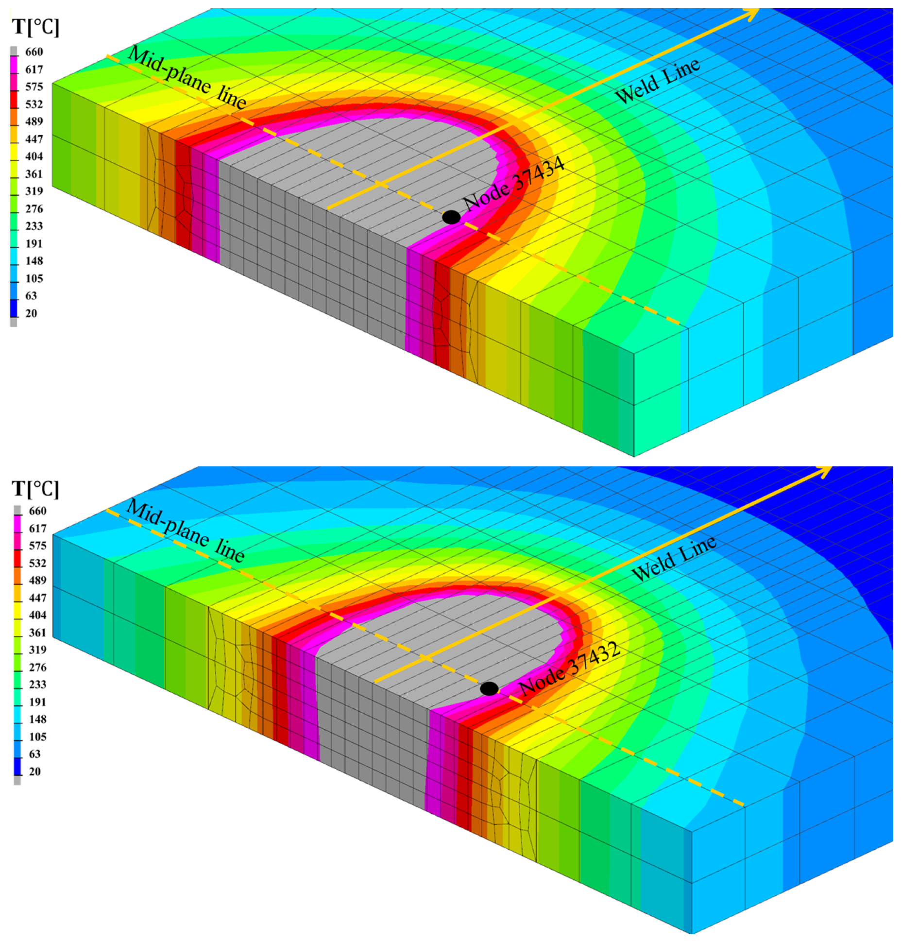
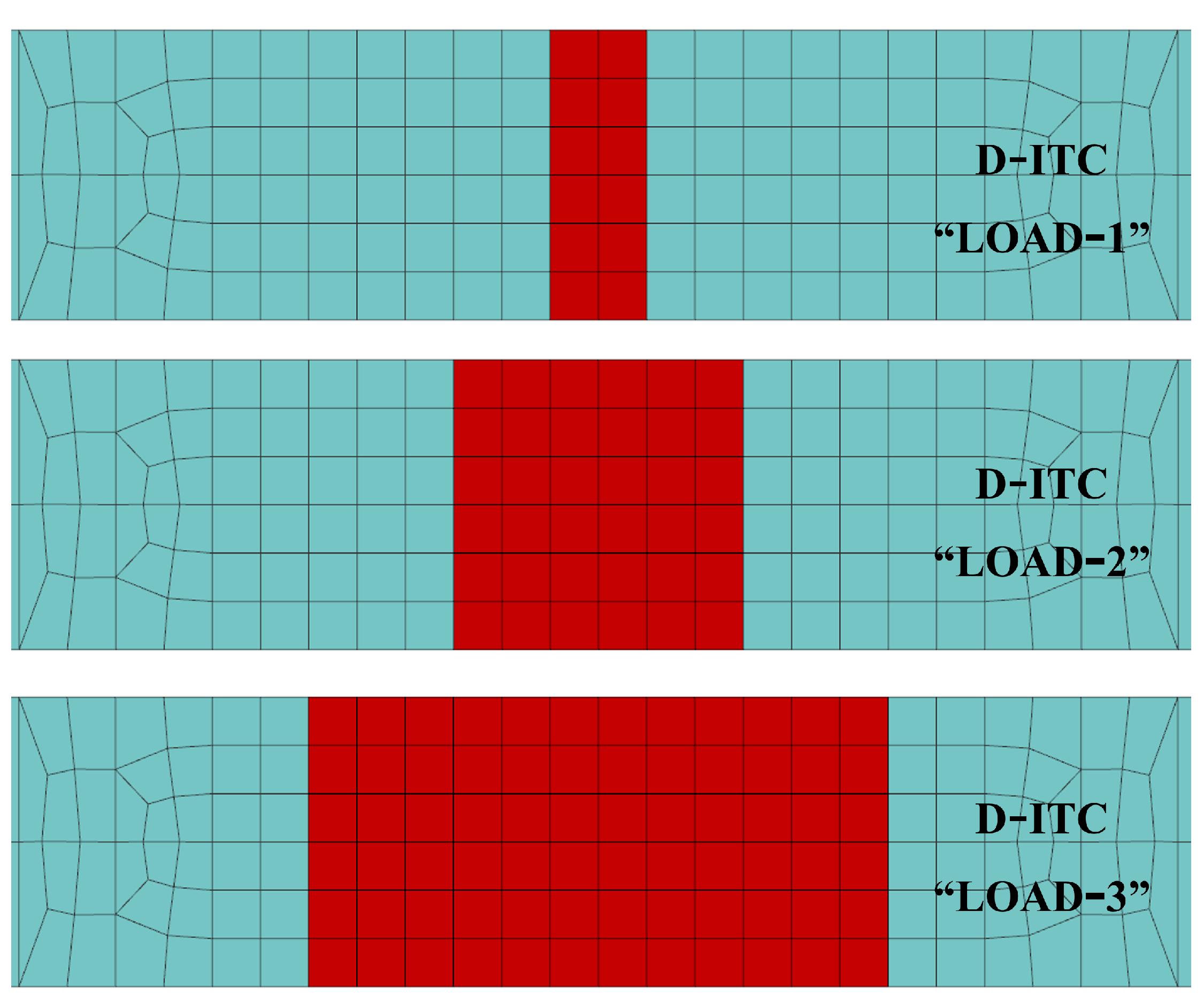
Figure 5.
Three different LOADs for D-ITC method.
3. Direct Imposed Thermal Cycle Method
The thermal cycle used in the T-ITC model is generally extracted from a calibrated MHS simulation. Nevertheless, it could also be derived directly from experimental data obtained through temperature measurements on the welded sheets. This is commonly achieved using contact thermocouples placed along a line perpendicular to the weld seam, covering the entire width of the heat-affected zone [9,39]. In this study, an innovative alternative is proposed: using an infrared (IR) camera to capture temperature data in real time during the welding process. This approach eliminates the need for MHS simulation or contact thermocouples and enables continuous acquisition of thermal cycle data, providing real and directly process-related temperauture measurements. Unlike the conventional iterative calibration process required by the MHS approach, the proposed Direct-Imposed Thermal Cycle (D-ITC) method integrates infrared thermography directly into the simulation workflow. This allows the experimentally measured thermal cycles to be imposed in the ITC model without the need for extensive iterative paramter tuning. Although the D-ITC method still requires calibration, it is significantly simpler (i.e., fewer input parameters) and faster than MHS calibration. The only parameter requiring adjustment is the LOAD - the area to which the thermal cycle is applied - based on its influence on mechanical distortion outputs. Figure 5 presents three different LOAD configurations used for D-ITC calibration. Consequently, all LOAD elements are subjected to the same thermal cycle, receiving the same thermal input during both the heating and cooling stages. The extent of distortion in the component is directly influenced by the size of the LOAD area, since it defines the effective heating zone. Given that a single thermo-metallurgical-mechanical simulation run takes approximately 24 minutes, the total estimated time to complete the D-ITC calibration process was around 90 minutes—significantly faster than traditional approaches.
3.1. IR Camera Monitoring
A FLIR A700 microbolometric infrared camera equipped with an FOL18H lens was used to monitor the laser welding process. This camera featured a long-wave sensor (7–14 ), making it compatible with laser welding sources operating near wavelength. It was positioned 600 from the weld seam at a 40° angle to the horizontal plane, providing an IFOV of 676 . The temperature measurement range is 0–700 °C, and the system was set at a fixed distance of 1.00 m from the specimen to ensure consistent data acquisition. For butt joint welds, the specimens were carefully oriented to ensure an acceptable view and spatial resolution. Thermal data was post-processed using Flir Research Studio software.
Calibration of the IR system was necessary because the surface thermal emissivity varied strongly with temperature. By identifying an isothermal pleteau corresponding to the solid-liquid phase transition (around 650–670°C) and comparing it with literature values for aluminum 6061 and 6082 alloys, the surface emissivity was set to 0.35.
To extract a thermal cycle suitable for use in the simulation (comparable to that obtained from the MHS model), the thermograms were analyzed to identify a region located just outside the molten zone. The thermal history in this region was then extracted and used as input for the D-ITC model.
4. Experimental Results
This section presents the experimental tests and numerical simulations used to validate both the conventional and proposed modeling approaches. Comparisons focus on cross-sectional metallography, thermal distribution, and mechanical distortions.
4.1. Materials and Experimental Methodology
To demonstrate the effectiveness of the proposed approach, two laser welding experiments were performed to acquire reference data.
The laser beam source was a diode-laser (Laserline LDF 4000-40) with a maximum power of 4 kW and two wavelengths of 1020 and 1060 ±10 nm. The welding head (Laserline OTS-5) was mounted on a 6-axis ABB IRB 2400 industrial robot. Welding was conducted on 1.5 mm thick Al 6061-T6 plates, each measuring mm, in a butt configuration. Prior to welding, the joint area was sanded and polished to remove contaminats (grease and dirt traces), and then cleaned thoroughly with acetone. The two aluminum plates were clamped to ensure a zero-gap joint, as illustrated in Figure 6). The laser beam was oriented perpendicular to the plate surface, and the focal point was adjusted to 3 mm above the plate surface, resulting in a beam spot diameter of 1.2 mm. Neither shielding gas nor filler material was used during welding. The laser power was set at 2800 W. The two welding experiments differed only in the welding speed: 35 and 50 for samples 1 and 2, respectively.
To examine the joint geometry, a cross-sectional specimen was prepared by cutting through the weld zone. The samples was hot-mounted, polished to achieve a homogeneous surface finish, and then chemically etched using Keller’s reagent for metallographic analysis (microscope ZEISS Axiovert a1). Subsequently, the molten pool geometry was measured using the software ImageJ. Post-weld distortion of the aluminum sheets was assessed using a direct contact profilometer. One side of the sheet was fixed, as shown in Figure 7, and the measurement line was oriented at a 90° angle to the weld seam, positioned at the midpoint of the sheet.
4.2. Numerical Solver
Considering the complexity of the welding process and focusing on understanding the effect of heat input on mechanical distortion, the models described in Section 2.1 were numerically solved through FEM analysis. A single FEM model was employed for both samples, with varying input parameters, and simulations were carried out using SYSWELD software in two steps: a thermo-metallurgical simulation followed by a mechanical simulation [39,42]. Material porperties and model parameters were selected according to the SYSWELD database. The conductive heat transfer was set to , and surface emissivity as .
Using Visual-Mesh (SYSWELD) module, mesh was defined with 54,400 8-node hexahedral linear 3D prism elements representing the solid domain; 36,544 4-node rectangular linear 2D elements to model heat exchange with the environment; and 200 1D line elements to define both the welding trajectory and reference lines.
Figure 2 provides an overview of the model, including spatial orientation, clamping positions, and Heat Affected Zone (HAZ) mesh appearance. The coordinate system is defined as follows: x-axis corresponds to the welding direction, the y-axis the direction of the weldment with, and the z-axis the direction of weld pool penetration (i.e., thickness). Mesh density was refined in thermally critical regions to ensure accuracy while maintaining reasonable computational time. Specifically, finer mesh grids of mm were used in the HAZ, with a transition to coarser center-concentric biased elemenst beyond the Fusion Zone (FZ) [8]. Numerical model computation used the Broyden-Fletcher-Goldfarb-Shanno (BFGS) algorithm to ensure convergence and numerical stability [9].
In the same welding conditions, thinner plates are more prone to longitudinal and transverse shrinkage, as well as angular distortions due to thermal during volumetric expansion and contraction during welding [43]). In FEM simulations based on small deformation theory - where strain is linearly dependent on displacement - large distortions are often underestimated. However, the interaction of large distortions (longitudinal, transverse, and bidirectional angular) leads to buckling phenomenon. In large distortion theory, instead, strain is a nonlinear function of displacement. The nonlinear geometry option of SYSWELD accounts for such behavior, though some discrepancy between experimental and FEM numerical results still remains [44]. In this work, the bending optimized function of SYSWELD was used to improve the accuracy of distortion computation. Standard hexahedral elements are limited in accurately capturing bending kinematics. This limitation is addressed by using incompatible mode elements, which incorporate additional shape functions to better modeling bending behavior [45]. As a result, all solid elements, except those in the HAZ, were defined as type 2 (i.e., incompatible mode elements) to enhance the accuracy of distortion computations.
4.3. Cross-Section Comparison
Figure 8 illustrates the criteria used for measuring the melt pool and presents a comparative analysis between the metallographic cross-sections of the laser-welded aluminum alloys (Sample 1 and Sample 2) and the corresponding results from MHS simulations. Both experimental and simulated results clearly display the Base Metal (BM) and Fusion Zone (FZ). Table 1 summarizes the fusion zone dimensions obtained from the cross-sectional analysis.
The calibrated model exhibits only minor differences between the experimental and FEM results for the weld widths and . In Sample 2, a smaller fusion zone was observed, which can be attributed to the lower heat input per unit length caused by the higher welding speed.
4.4. Thermal Analysis Results
Thermal distribution during the welding process was measured through thermographic monitoring. Figure 9 shows a representative frame from the thermal video captured during the experiment. The boundary of the weld pool can be identified from the temperature distribution, with the white region indicating temperatures at or above the melting point of aluminum, approximately 660 °C. It is worth noting that temperature acquisition through an IR thermal camera relies on the knowledge of the material emissivity, which varies with its physical state. In the weld pool, the emissivity of liquid aluminum differs from that of its solid form, introducing potential error in measuring temperature inside the weld pool. Despite this limitation, the frame in Figure 9 clearly shows temperature gradient from the outer edges of the metal sheets (cooler, darker regions) toward the weld center (hotter, lighter), where the laser is focused. (i.e., about 660 °). The gray region at the center represents pixel saturation due to the upper temperature limit of the IR camera. However, in this study, the primary aim is on the thermal behavior outside the weld pool, where emissivity is more stable and temperature measurements are considered reliable.

Table 1.
Comparison between FEM and experimental results.
| Sample | FEM (mm) | Experiment (mm) | ||||
|---|---|---|---|---|---|---|
| W1 | W2 | W1 | W2 | |||
| 1 | 3.22 | 3.18 | 3.20 | 3.20 | ||
| 2 | 2.65 | 2.30 | 2.64 | 2.29 | ||
Thermal cycles were extracted from both the MHS simulation and the thermographic measurements taken at the boundary of the molten zone. To validate the proposed methodology, the thermal cycles adopted for T-ITC and D-ITC was compared with those obtained from the MHS simulation. The strong correlation between these thermal profiles, as shown in Figure 10, confirms the ability of the simulation framework to accurately capture the thermal dynamics of the welding process. Following the procedures outlined in Section 2.3 and Section 3, the thermal cycles given in Figure 11, which were derived from the thermal curves depicted in Figure 10, were imposed on the T-ITC and D-ITC numerical models.
The simulation successfully captures the distinct thermal cycles observed in the two samples, accurately reflecting the different heat inputs applied during welding. These differences are consistent with observations from thermographic analysis. To further investigate spatial temperature variations, thermal cycles were extracted from three nodes on the top surface of the model, aligned along the mid-plane line (in the transverse direction): P1, P2, and P3, positioned at 1.5 mm, 2.5 mm, and 4.73 mm from the weld centerline, respectively. The resulting thermal cycles were then compared. Figure 12 shows the thermal cycles extracted for both sample 1 and sample 2, labeled as V35 and V50, respectively, to illustrate the thermal cycle behavior at different distances from the weld centerline. As expected, peak temperature decreases with increasing distance from the weld centerline, consistent with standard thermal diffusion behavior.
4.5. Mechanical Analysis Results
During welding, the weldment temperature is raised above the liquidus temperature to ensure proper melting of the joint area. The large temperature gradient experienced during the heating and cooling stages causes significant volumetric expansion and contraction, leading to metallurgical and mechanical transformations within the material. The thermal data computed from the thermo-metallurgical simulation serve as input for the mechanical analysis, enabling the prediction of welding-induced deformations, including potential buckling behavior and residual stresses, particularly for thin aluminum alloy components. To account for these effects accurately, all numerical models were computed with nonlinear geometry effects, as recommended in [44]. The mechanical performance of the numerical models was assessed mainly by analyzing the vertical displacement and the distortion angle resulting from the welding process for both samples.
Figure 13 illustrates the method used to assess the distortion angle from the simulations and to compare it with the actual distortions measured using a profilometer. Table 2 summarizes the comparison between the numerical predicted distortion angle and the experimental measurements.
For both samples, the numerical prediction of angular distortions match the experimental measurements, with estimation errors consistently below 0.3 %. A slightly more accurate distortion estimation was obtained for Sample 1, which was produced at a lower welding speed. Notably, the distortion estimation errors are comparable between the traditional simulation methods or the proposed technique. This demonstrates the efficiency of the D-ITC approach, as it provides reasonably similar results in about 90 minutes, significantly faster than the over 10 hours required by traditional simulations methods.
The excellent agreement between simulation and experimental results across both thermal and mechanical parameters confirms the validity of our simulation approach, whether using conventional iterative calibration or the proposed method based on thermal camera data.
5. Conclusions
This study proposes an FEM simulation approach to predict the thermal and distortion behaviors during laser welding of thin aluminum alloy sheets. A comparative analysis between experimental observations and simulation results demonstrates strong agreement, particularly in reproducing thermal cycles and distortion profiles.
A key innovation in this work is the use of IR thermal camera data to impose thermal cycles directly in the simulation, thereby eliminating the need for calibrating a moving heat source model. This significantly simplifies the computational process and speeds up the tuning procedure. Consequently, the predictive accuracy of the FEM simulations is improved, enabling more reliable and efficient modeling. The proposed algorithm is particularly applicable to industries such as automotive, where it can streamline production workflow and improve weld quality by mitigating the reliance on time-consuming and resource-intensive calibration procedures. Experimental validation confirms that the proposed method achieves accuracy comparable to traditional simulation approaches, while reducing the computation time by more than 10 hours. This proves the efficiency of the proposed simulation approach.
In summary, the integration of IR thermography with FEM simulations represents a meaningful advancement in the predictive modeling of laser welding processes. This approach improves both the accuracy and reliability of simulations, providing a valuable tool to optimize manufacturing processes and supporting the automotive industry in the pursuit of lightweight and high-performance components.
Declaration of Competing Interest
The authors declare that they have no known competing financial interests or personal relationships that could have appeared to influence the work reported in this paper.
Data availability
Data will be made available on request.
Acknowledgments
The authors gratefully acknowledge the support of ESI Group and J-Tech@Polito, an advanced joining technologies research center at Politecnico di Torino (http://www.j-tech.polito.it/).
References
- Zhang, W.; Xu, J. Advanced lightweight materials for Automobiles: A review. Materials & Design 2022, 221, 110994. [Google Scholar] [CrossRef]
- Basile, D.; Sesana, R.; De Maddis, M.; Borella, L.; Russo Spena, P. Investigation of Strength and Formability of 6016 Aluminum Tailor Welded Blanks. Metals 2022, 12, 1593. [Google Scholar] [CrossRef]
- Aminzadeh, A.; Silva Rivera, J.; Farhadipour, P.; Ghazi Jerniti, A.; Barka, N.; El Ouafi, A.; Mirakhorli, F.; Nadeau, F.; Gagné, M.O. Toward an intelligent aluminum laser welded blanks (ALWBs) factory based on industry 4.0; a critical review and novel smart model. Optics & Laser Technology 2023, 167, 109661. [Google Scholar] [CrossRef]
- Bunaziv, I.; Akselsen, O.M.; Ren, X.; Nyhus, B.; Eriksson, M. Laser Beam and Laser-Arc Hybrid Welding of Aluminium Alloys. Metals 2021, 11, 1150. [Google Scholar] [CrossRef]
- Stavridis, J.; Papacharalampopoulos, A.; Stavropoulos, P. Quality assessment in laser welding: a critical review. The International Journal of Advanced Manufacturing Technology 2018, 94, 1825–1847. [Google Scholar] [CrossRef]
- Li, Y.; Wang, Y.; Yin, X.; Zhang, Z. Laser welding simulation of large-scale assembly module of stainless steel side-wall. Heliyon 2023, 9, e13835. [Google Scholar] [CrossRef]
- Anca, A.; Cardona, A.; Risso, J.; Fachinotti, V.D. Finite element modeling of welding processes. Applied Mathematical Modelling 2011, 35, 688–707. [Google Scholar] [CrossRef]
- Kik, T. Calibration of Heat Source Models in Numerical Simulations of Welding Processes. Metals 2024, 14, 1213. [Google Scholar] [CrossRef]
- Mohan, A.; Franciosa, P.; Dai, D.; Ceglarek, D. A novel approach to control thermal induced buckling during laser welding of battery housing through a unilateral N-2-1 fixturing principle. Journal of Advanced Joining Processes 2024, 10, 100256. [Google Scholar] [CrossRef]
- Chuang, T.C.; Lo, Y.L.; Tran, H.C.; Tsai, Y.A.; Chen, C.Y.; Chiu, C.P. Optimization of Butt-joint laser welding parameters for elimination of angular distortion using High-fidelity simulations and Machine learning. Optics & Laser Technology 2023, 167, 109566. [Google Scholar] [CrossRef]
- Yan, H.; Zeng, X.; Cui, Y.; Zou, D. Numerical and experimental study of residual stress in multi-pass laser welded 5A06 alloy ultra-thick plate. Journal of Materials Research and Technology 2024, 28, 4116–4130. [Google Scholar] [CrossRef]
- Pyo, C.; Kim, J.; Kim, Y.; Kim, M. A study on a representative heat source model for simulating laser welding for liquid hydrogen storage containers. Marine Structures 2022, 86, 103260. [Google Scholar] [CrossRef]
- Murua, O.; Arrizubieta, J.; Lamikiz, A.; Schneider, H. Numerical simulation of a laser beam welding process: From a thermomechanical model to the experimental inspection and validation. Thermal Science and Engineering Progress 2024, 55, 102901. [Google Scholar] [CrossRef]
- Walker, T.; Bennett, C. An automated inverse method to calibrate thermal finite element models for numerical welding applications. Journal of Manufacturing Processes 2019, 47, 263–283. [Google Scholar] [CrossRef]
- Speka, M.; Matteï, S.; Pilloz, M.; Ilie, M. The infrared thermography control of the laser welding of amorphous polymers. NDT & E International 2008, 41, 178–183. [Google Scholar] [CrossRef]
- Bagavathiappan, S.; Lahiri, B.; Saravanan, T.; Philip, J.; Jayakumar, T. Infrared thermography for condition monitoring – A review. Infrared Physics & Technology 2013, 60, 35–55. [Google Scholar] [CrossRef]
- Razza, V.; Santoro, L.; De Maddis, M. Gradient-based image generation for thermographic material inspection. Applied Thermal Engineering 2025, 268, 125900. [Google Scholar] [CrossRef]
- Santoro, L.; Sesana, R.; Molica Nardo, R.; Curá, F. Infrared in-line monitoring of flaws in steel welded joints: a preliminary approach with SMAW and GMAW processes. The International Journal of Advanced Manufacturing Technology 2023, 128, 2655–2670. [Google Scholar] [CrossRef]
- Santoro, L.; Razza, V.; De Maddis, M. Frequency-based analysis of active laser thermography for spot weld quality assessment. The International Journal of Advanced Manufacturing Technology 2024, 130, 3017–3029. [Google Scholar] [CrossRef]
- Santoro, L.; Razza, V.; De Maddis, M. Nugget and corona bond size measurement through active thermography and transfer learning model. The International Journal of Advanced Manufacturing Technology 2024, 133, 5883–5896. [Google Scholar] [CrossRef]
- Santoro, L.; Sesana, R. A pilot study using flying spot laser thermography and signal reconstruction. Optics and Lasers in Engineering 2025, 188, 108901. [Google Scholar] [CrossRef]
- Sesana, R.; Santoro, L.; Curà, F.; Molica Nardo, R.; Pagano, P. Assessing thermal properties of multipass weld beads using active thermography: microstructural variations and anisotropy analysis. The International Journal of Advanced Manufacturing Technology 2023, 128, 2525–2536. [Google Scholar] [CrossRef]
- Brüggemann, G.; Mahrle, A.; Benziger, T. Comparison of experimental determined and numerical simulated temperature fields for quality assurance at laser beam welding of steels and aluminium alloyings. NDT & E International 2000, 33, 453–463. [Google Scholar] [CrossRef]
- Menaka, M.; Vasudevan, M.; Venkatraman, B.; Raj, B. Estimating bead width and depth of penetration during welding by infrared thermal imaging. Insight - Non-Destructive Testing and Condition Monitoring 2005, 47, 564–568. [Google Scholar] [CrossRef]
- Hellinga, M.C.; Huissoon, J.P.; Kerr, H.W. Identifying weld pool dynamics for gas metal arc fillet welds. Science and Technology of Welding and Joining 1999, 4, 15–20. [Google Scholar] [CrossRef]
- Vasilev, M.; MacLeod, C.N.; Loukas, C.; Javadi, Y.; Vithanage, R.K.W.; Lines, D.; Mohseni, E.; Pierce, S.G.; Gachagan, A. Sensor-Enabled Multi-Robot System for Automated Welding and In-Process Ultrasonic NDE. Sensors 2021, 21, 5077. [Google Scholar] [CrossRef]
- Nguyen, H.L.; Van Nguyen, A.; Duy, H.L.; Nguyen, T.H.; Tashiro, S.; Tanaka, M. Relationship among Welding Defects with Convection and Material Flow Dynamic Considering Principal Forces in Plasma Arc Welding. Metals 2021, 11, 1444. [Google Scholar] [CrossRef]
- Zhu, C.; Cheon, J.; Tang, X.; Na, S.J.; Cui, H. Molten pool behaviors and their influences on welding defects in narrow gap GMAW of 5083 Al-alloy. International Journal of Heat and Mass Transfer 2018, 126, 1206–1221. [Google Scholar] [CrossRef]
- Filyakov, A.E.; Sholokhov, M.A.; Poloskov, S.I.; Melnikov, A.Y. The study of the influence of deviations of the arc energy parameters on the defects formation during automatic welding of pipelines. In Proceedings of the IOP Conference Series: Materials Science and Engineering, 2020, Vol. 966. [CrossRef]
- Aucott, L.; Huang, D.; Dong, H.B.; Wen, S.W.; Marsden, J.A.; Rack, A.; Cocks, A.C.F. Initiation and growth kinetics of solidification cracking during welding of steel. Scientific Reports 2017, 7, 40255. [Google Scholar] [CrossRef]
- Hong, Y.; Yang, M.; Chang, B.; Du, D. Filter-PCA-Based Process Monitoring and Defect Identification During Climbing Helium Arc Welding Process Using DE-SVM. IEEE Transactions on Industrial Electronics 2023, 70, 7353–7362. [Google Scholar] [CrossRef]
- D’Accardi, E.; Chiappini, F.; Giannasi, A.; Guerrini, M.; Maggiani, G.; Palumbo, D.; Galietti, U. Online monitoring of direct laser metal deposition process by means of infrared thermography. Progress in Additive Manufacturing 2024, 9, 983–1001. [Google Scholar] [CrossRef]
- Zhang, C.; Li, X.; Gao, M. Effects of circular oscillating beam on heat transfer and melt flow of laser melting pool. Journal of Materials Research and Technology 2020, 9, 9271–9282. [Google Scholar] [CrossRef]
- Zhou, Q.; Rong, Y.; Shao, X.; Jiang, P.; Gao, Z.; Cao, L. Optimization of laser brazing onto galvanized steel based on ensemble of metamodels. Journal of Intelligent Manufacturing 2018, 29, 1417–1431. [Google Scholar] [CrossRef]
- Mirapeix, J.; García-Allende, P.; Cobo, A.; Conde, O.; López-Higuera, J. Real-time arc-welding defect detection and classification with principal component analysis and artificial neural networks. NDT & E International 2007, 40, 315–323. [Google Scholar] [CrossRef]
- Zhang, H.; Chen, Z.; Zhang, C.; Xi, J.; Le, X. Weld Defect Detection Based on Deep Learning Method. In Proceedings of the 2019 IEEE 15th International Conference on Automation Science and Engineering (CASE); 2019; pp. 1574–1579. [Google Scholar] [CrossRef]
- Sarkar, S.S.; Das, A.; Paul, S.; Mali, K.; Ghosh, A.; Sarkar, R.; Kumar, A. Machine learning method to predict and analyse transient temperature in submerged arc welding. Measurement 2021, 170, 108713. [Google Scholar] [CrossRef]
- Bergman, T.L.; Lavine, A.S.; Incropera, F.P.; DeWitt, D.P. Fundamentals of Heat and Mass Transfer, 8th Edition; John Wiley & Sons, Inc., 2018.
- Kik, T. Computational Techniques in Numerical Simulations of Arc and Laser Welding Processes. Materials 2020, 13, 608. [Google Scholar] [CrossRef]
- Unni, A.K.; Vasudevan, M. Computational fluid dynamics simulation of hybrid laser-MIG welding of 316 LN stainless steel using hybrid heat source. International Journal of Thermal Sciences 2023, 185, 108042. [Google Scholar] [CrossRef]
- Vargas, J.A.; Torres, J.E.; Pacheco, J.A.; Hernandez, R.J. Analysis of heat input effect on the mechanical properties of Al-6061-T6 alloy weld joints. Materials & Design (1980-2015) 2013, 52, 556–564. [Google Scholar] [CrossRef]
- Marques, E.S.V.; Silva, F.J.G.; Pereira, A.B. Comparison of Finite Element Methods in Fusion Welding Processes—A Review. Metals 2020, 10. [Google Scholar] [CrossRef]
- Long, H.; Gery, D.; Carlier, A.; Maropoulos, P. Prediction of welding distortion in butt joint of thin plates. Materials & Design 2009, 30, 4126–4135. [Google Scholar] [CrossRef]
- Vinoth, A.; Sivasankari, R. Numerical Simulation Studies in Tungsten Inert Gas Welding of Inconel 718 Alloy Sheet. Journal of Materials Engineering and Performance 2024. [Google Scholar] [CrossRef]
- Kožar, I.; Rukavina, T.; Ibrahimbegović, A. Method of Incompatible Modes – Overview and Application. GRAĐEVINAR 2018, 70, 19–29. [Google Scholar] [CrossRef]
Figure 1.
3D Gaussian truncated conical heat source model.
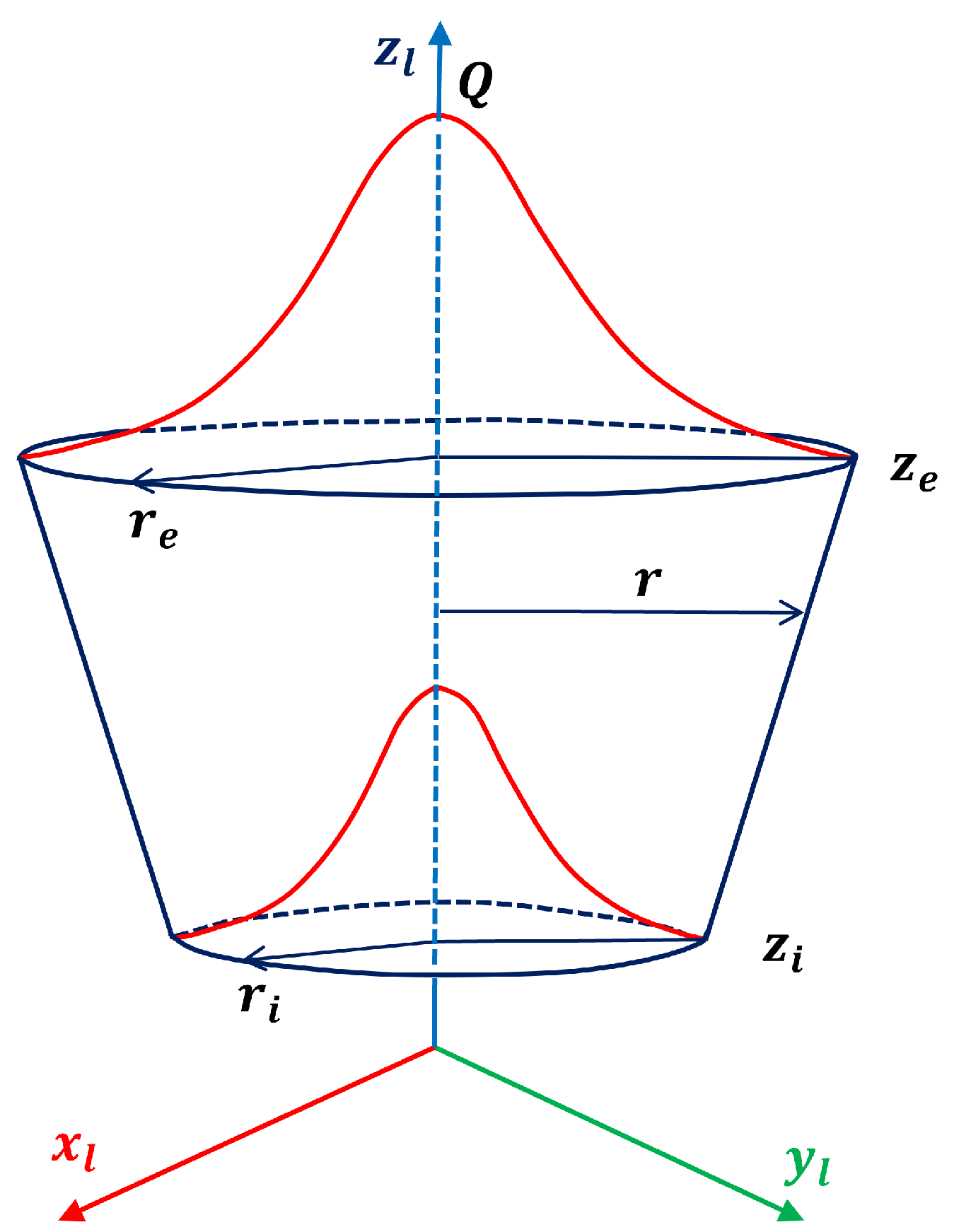
Figure 2.
Finite Element Model and Clamping Position.
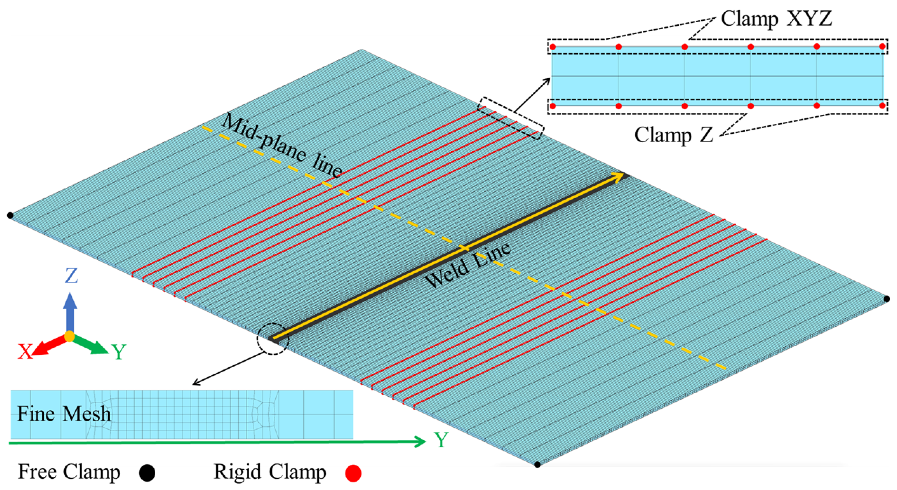
Figure 3.
Selected mesh elements (LOAD) heated by MHS.
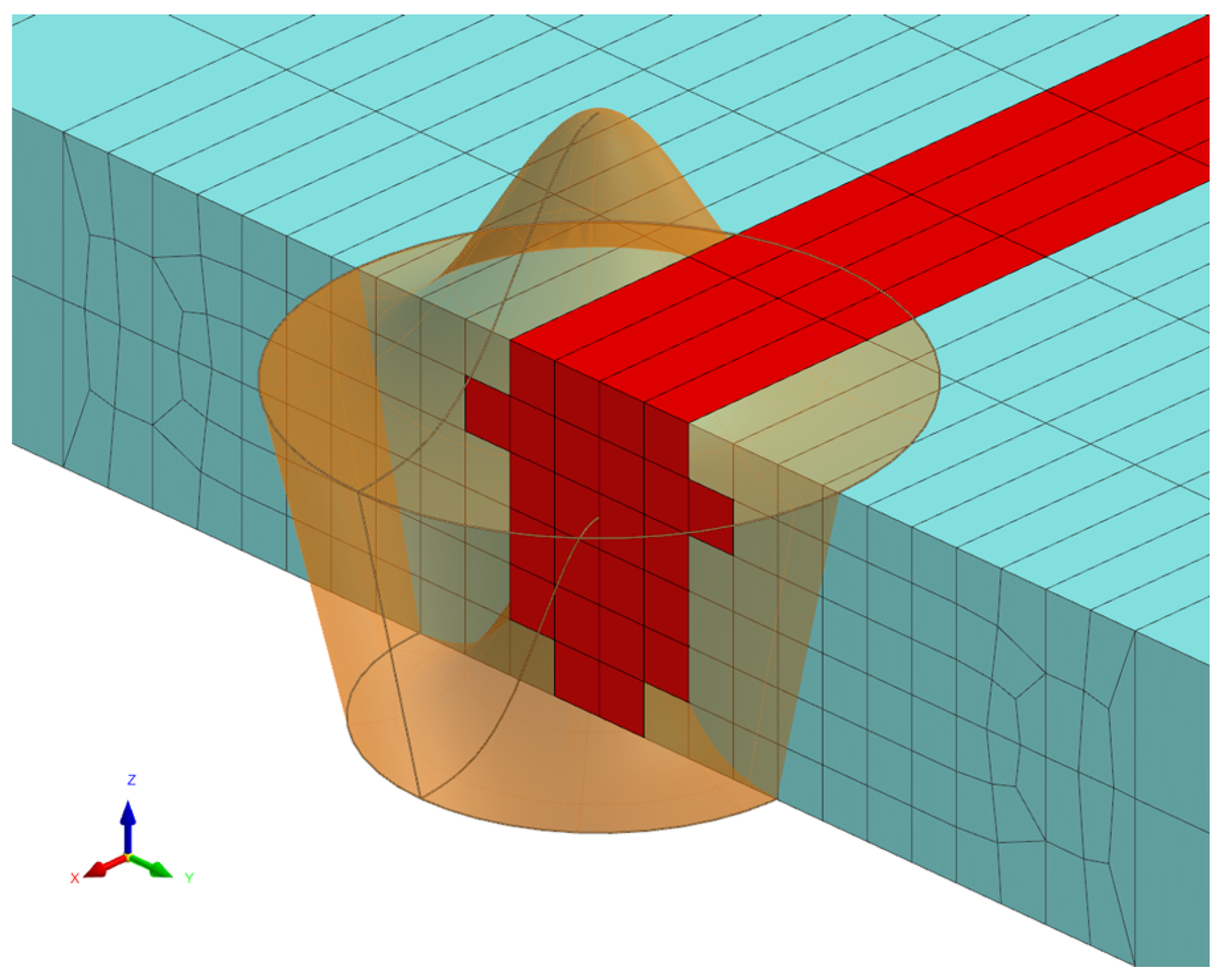
Figure 6.
Welding setup and thermal camera.
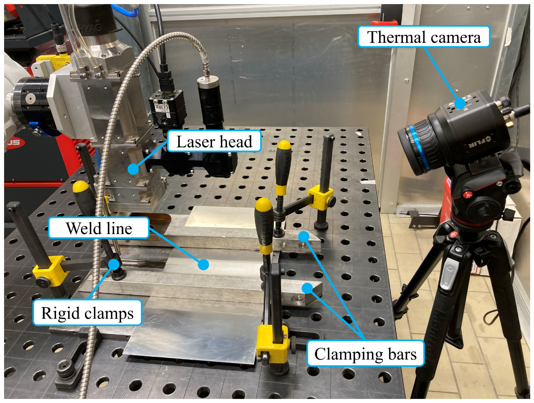
Figure 7.
Profilometer measurements set-up
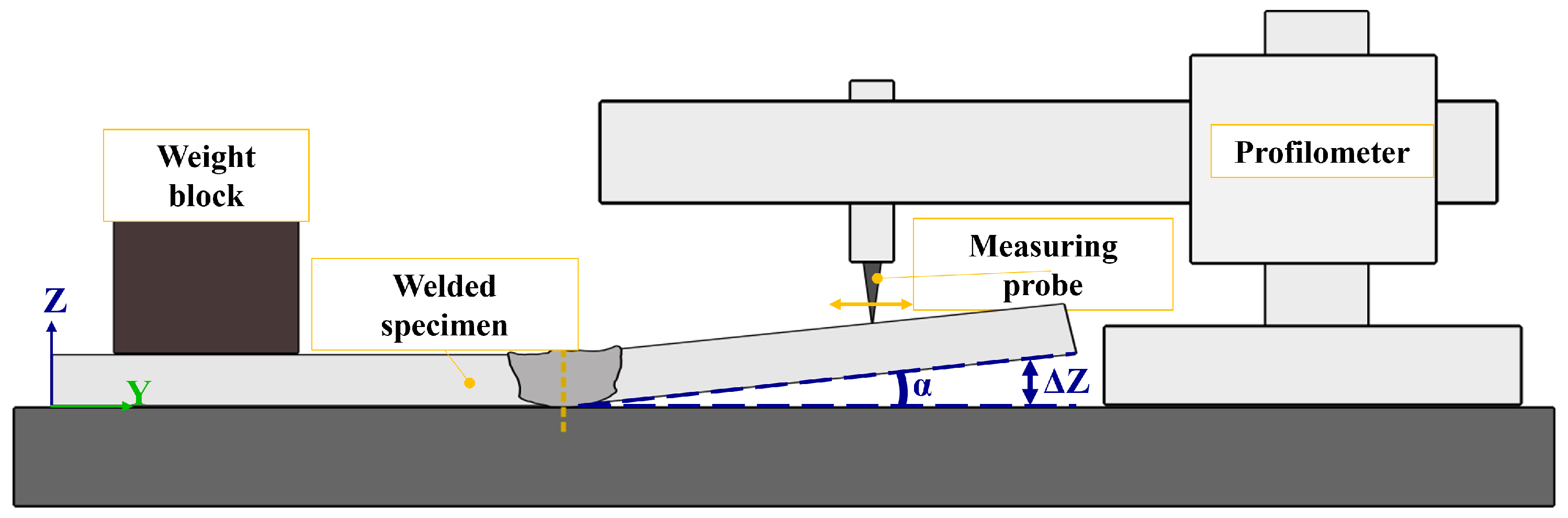
Figure 8.
Numerical and experimental melt pool morphology comparison: (a) Sample 1, (b) Sample 2. (c) Fusion zone measurements criteria.
Figure 8.
Numerical and experimental melt pool morphology comparison: (a) Sample 1, (b) Sample 2. (c) Fusion zone measurements criteria.
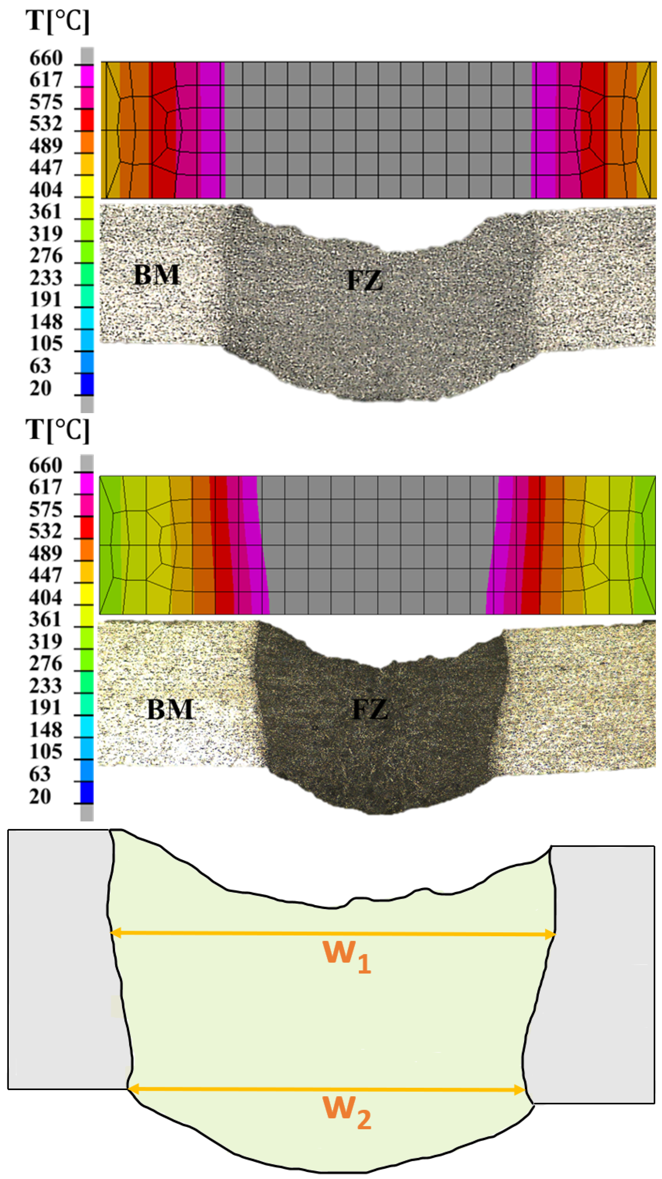
Figure 9.
Thermography map highlighting the weld pool.
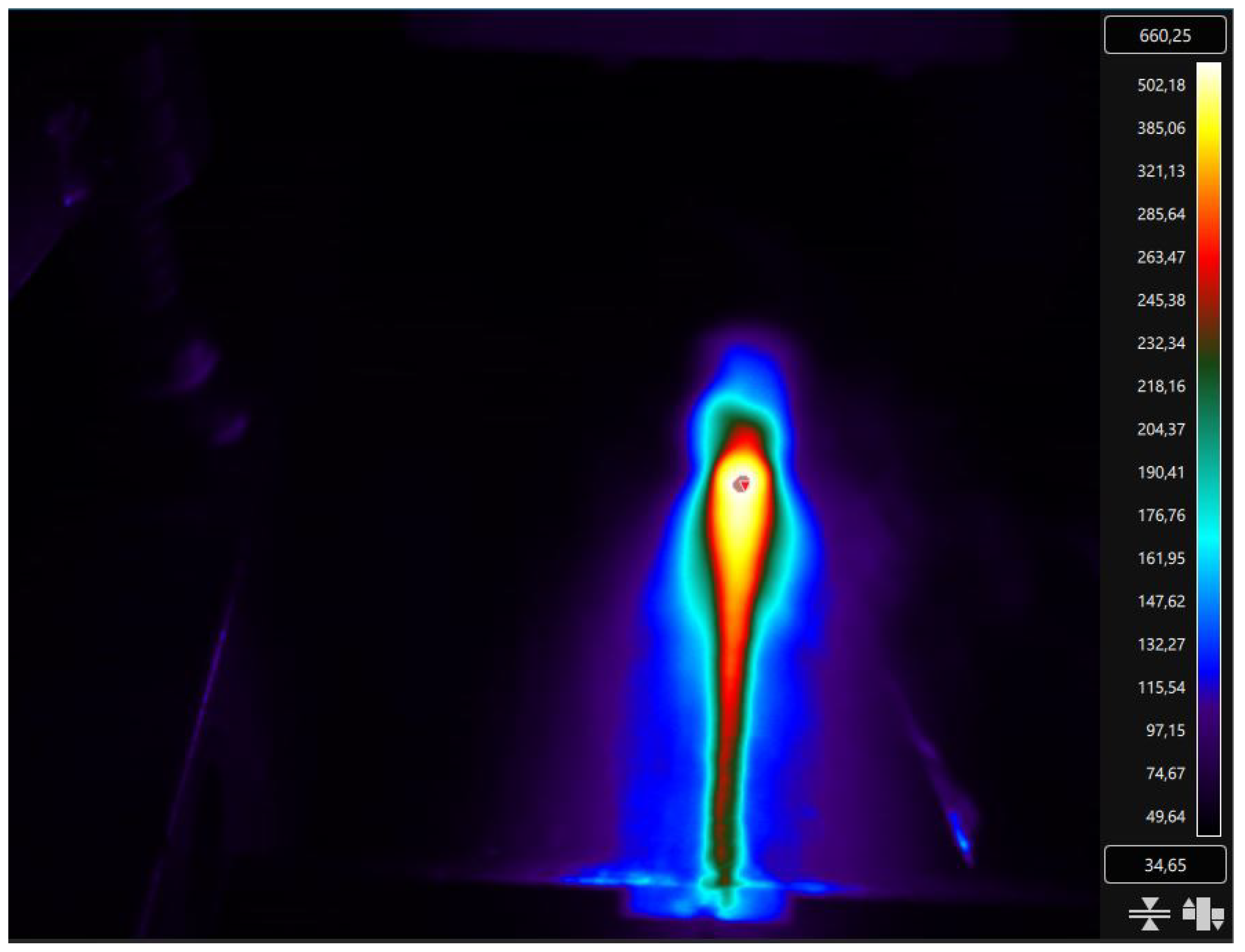
Figure 10.
Comparison of experimental and numerical thermal cycles.
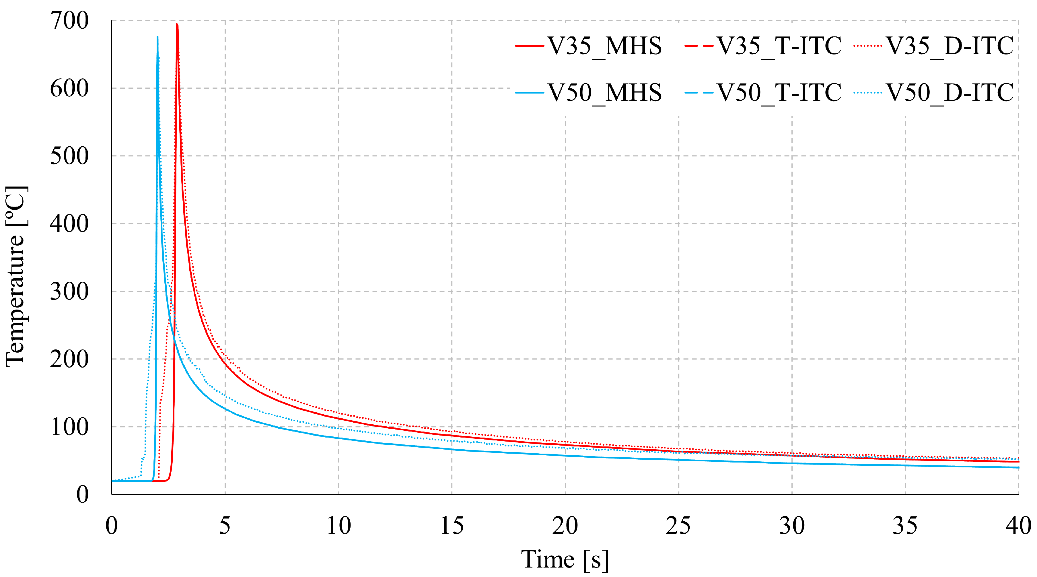
Figure 11.
Traditional and direct thermal cycles comparison.
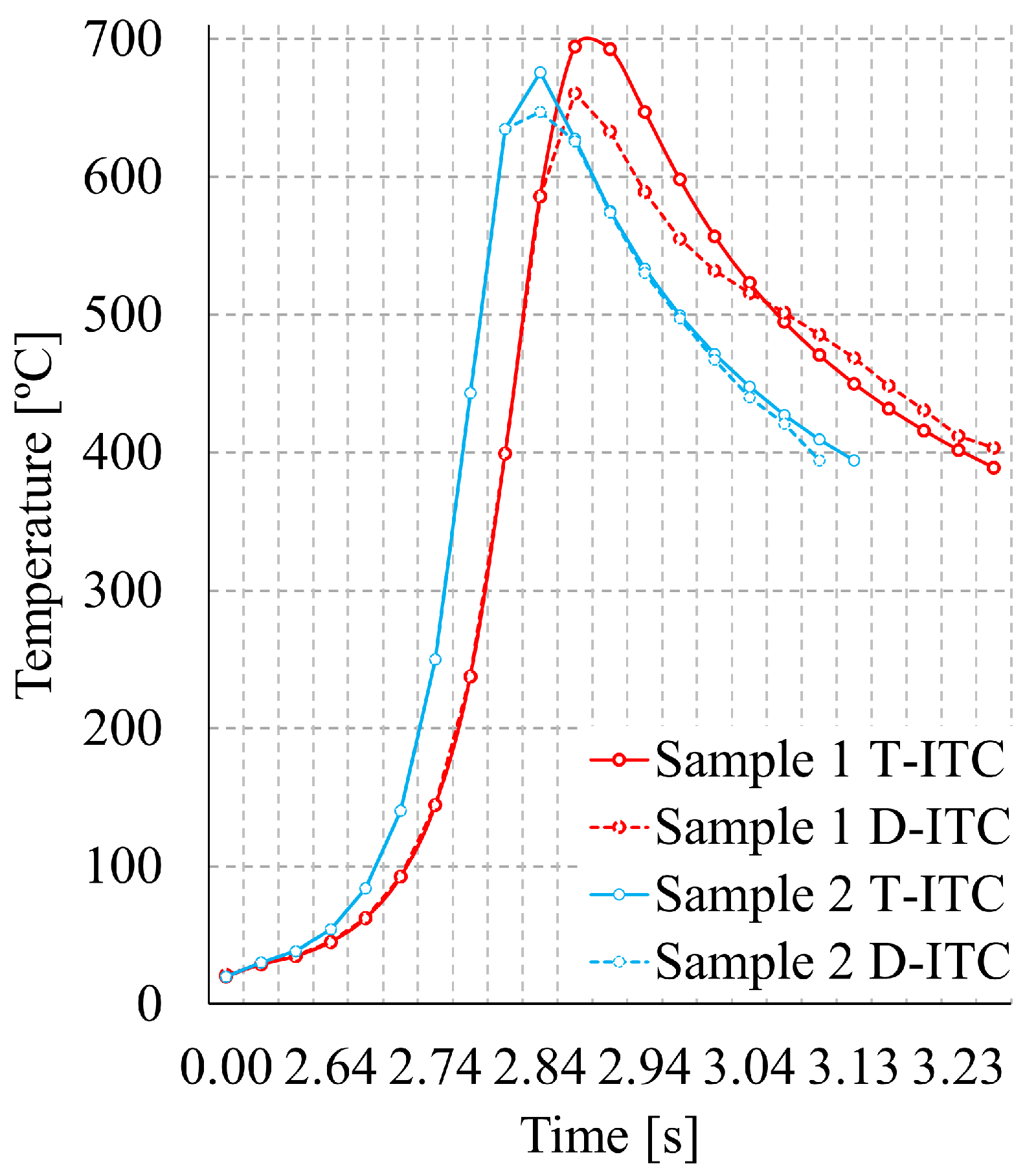
Figure 12.
Temperature evolution at different points along the central cross-section for two samples.
Figure 12.
Temperature evolution at different points along the central cross-section for two samples.
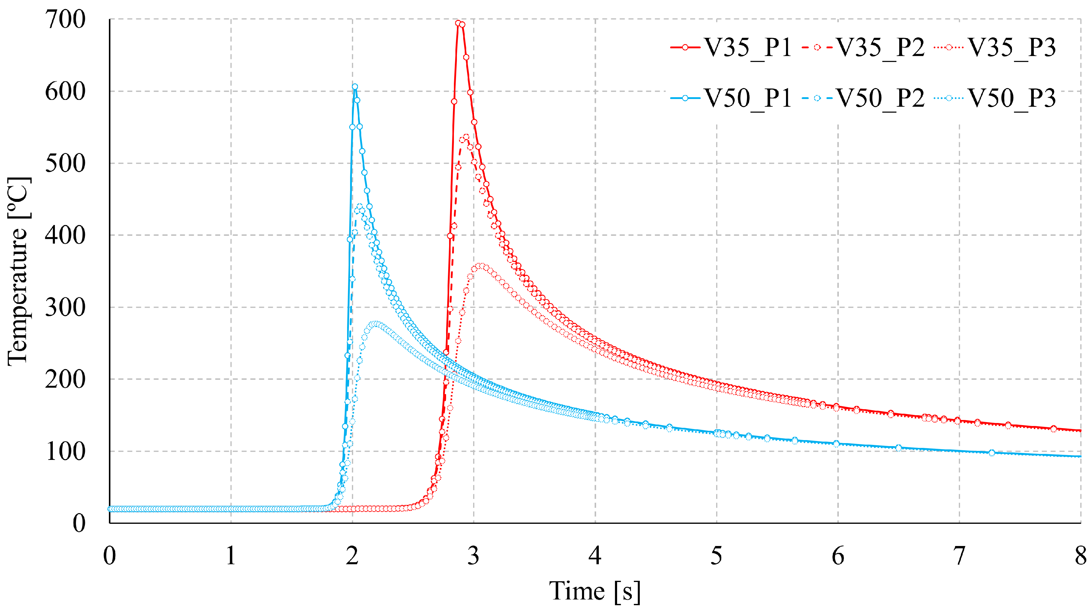
Figure 13.
Example of distortion angle calculation from simulation results.
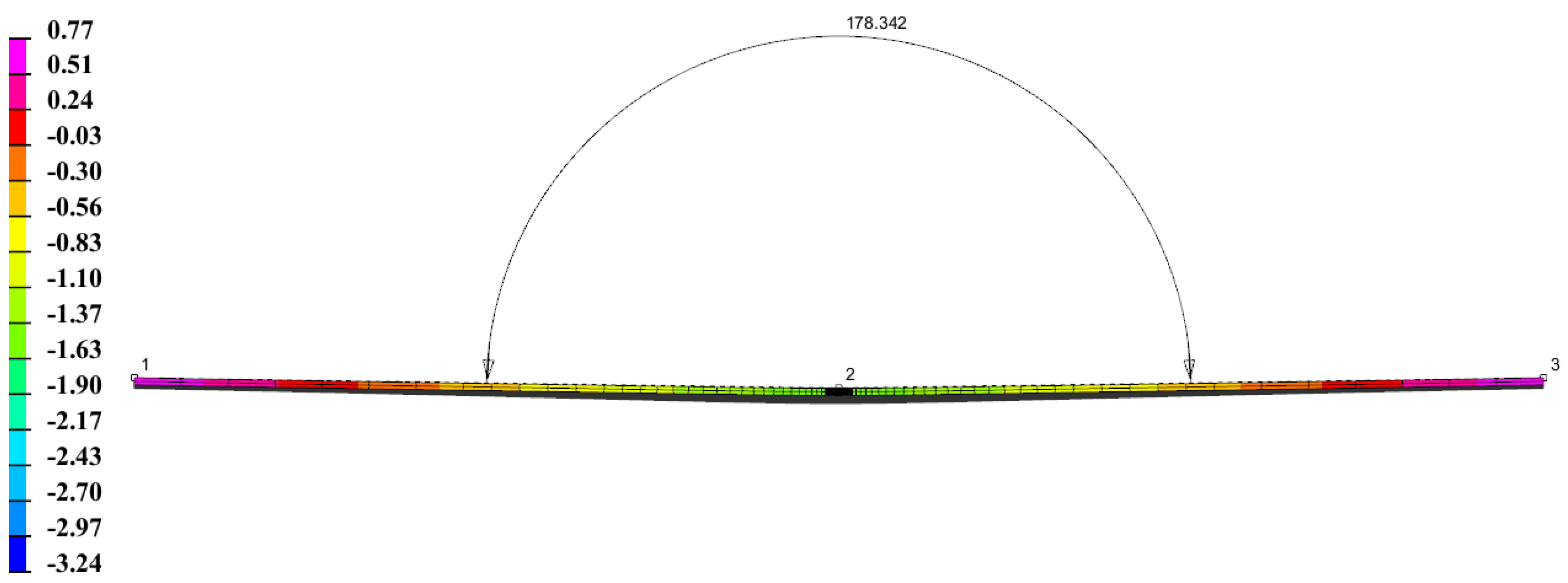
Table 2.
Distortion angle results: comparison between simulation models and experiment for sample 1 and sample 2.
Table 2.
Distortion angle results: comparison between simulation models and experiment for sample 1 and sample 2.
| Sample | Model | Angle (°) | Error (%) |
|---|---|---|---|
| 1 | MHS | 177.98 | 0.15 |
| T-ITC | 177.97 | 0.15 | |
| D-ITC | 177.92 | 0.18 | |
| Experiment | 178.24 | ||
| 2 | MHS | 178.43 | 0.22 |
| T-ITC | 178.37 | 0.25 | |
| D-ITC | 178.34 | 0.27 | |
| Experiment | 178.82 |
Disclaimer/Publisher’s Note: The statements, opinions and data contained in all publications are solely those of the individual author(s) and contributor(s) and not of MDPI and/or the editor(s). MDPI and/or the editor(s) disclaim responsibility for any injury to people or property resulting from any ideas, methods, instructions or products referred to in the content. |
© 2025 by the authors. Licensee MDPI, Basel, Switzerland. This article is an open access article distributed under the terms and conditions of the Creative Commons Attribution (CC BY) license (http://creativecommons.org/licenses/by/4.0/).
Copyright: This open access article is published under a Creative Commons CC BY 4.0 license, which permit the free download, distribution, and reuse, provided that the author and preprint are cited in any reuse.


