Algorithm for Describing Neuronal Electric Operation

1. Introduction

The brain, with its information processing capability, and finally, the mind, with its conscience and behavior, are still among the big mysteries of science. From the perspective of understanding neural computing, the large, coordinated projects spanning many years failed. A decade ago, it was targeted “The Human Brain Project should lay ...a new model of ...brain research, ...to achieve a new understanding of the brain ...and new brain-like computing technologies”. However, only new graphic user interfaces and libraries [1] have been prepared for the many-decades-old understanding; furthermore, "surprisingly, [among the winners of the supercomputer competition] there have been no brain-inspired massively parallel specialized computers" [2]. As the Brain Initiative summarized, "Yet for the most part, we still do not understand the brain’s underlying computational logic" [3].

On the occasion of the anniversary of Erwin Schrödinger’s famous book [4], we could revive the claim "The construction [of living matter] is different from anything we have yet tested in the physical laboratory." "It is working in a manner that cannot be reduced to the ordinary laws of physics". Even if we find the ’non-ordinary’ physical laws [5] that describe the phenomena of life, it is by no means certain that we will also have the mathematical methods and algorithms to describe them quantitatively. When Newton discovered that the complicated description of celestial mechanics and the Ptolemaic worldview had to be replaced by the law of universal gravitation, he had to create a new mathematical procedure (algorithm) that would serve as the basis for practical mathematical analysis. The theory of neural information processing also needs to revisit our notions of information and its processing [6,7,8].

The "new understanding" of the brain encompasses incorporating recent anatomical and physiological discoveries from the past few decades into the model, along with the correct (physically based) electrical and thermodynamic descriptions of the processes. As the observations revealed finer details of its operation, we have learned that the operation of the neuron is too complex to be described by a single physical process (and, what is more, even by a single discipline) using a model described by a single mathematical equation, we followed Feynman’s hint "Breaking down topics into digestible chunks and explaining them helps you identify gaps in your knowledge. This creates new neural pathways in your brain, which makes connecting ideas and concepts easier." [9] Our model divides neuron’s operation into stages (see [10], section 4) where different physical processes take place. Even within those stages, the intensity of different electrical contributions changes over time. It requires precise time handling, which can be ensured only by using ’non-ordinary’ time-handling technology and algorithms for simulation.

We formulate problems, provide their numerical solutions (including algorithms), and open the way for mathematics to provide analytical solutions. Our procedure is surely non-ordinary, yet it meets the requirement given by Feynman: [9] "an effective procedure is a set of rules telling you, moment by moment, what to do to achieve a particular end; it is an algorithm."

We know from the beginnings that "the language of the brain, not the language of mathematics" [11] and that "whatever the system [of the brain] is, it cannot fail to differ from what we consciously and explicitly consider mathematics" [12]; by adding that maybe the appropriate mathematical methods are not yet invented. "We so far lack principles to understand rigorously how computation is done" in living, or active, matter [13]. We also note that we lack principles of computation for large-scale, complex computing systems [14], especially when using them to imitate neuronal operation.

As [15] classified, "the term neuromorphic encompasses at least three broad communities of researchers, distinguished by whether they aim to emulate neural function (reverse-engineer the brain), simulate neural networks (develop new computational approaches), or engineer new classes of electronic device." We address the first class, indirectly touch the second, and discuss the third in [10]. Many methods and ideas, including half-understood and misleading ones, are used to imitate the brain’s operation. Unfortunately, all these communities inherited the wrong ideas above, see [10]. We aim to provide an algorithmic-level description of the genuine processes of neuronal operation (see [10], Section 4) for these fields, facilitating a better understanding. Mainly because "the operation of our brain differs vastly from that of human-made computing systems, both in terms of topology and in the way it processes information" [16], a precise description of the way of mapping one’s operation (including their temporal behavior) to the other is needed.

At the level of abstraction we use, one does not need to consider all biological details since "despite the extraordinary diversity and complexity of neuronal morphology and synaptic connectivity, the nervous systems adopt a number of basic principles"  [17] and we proceed along those basic principles, emphasizing the need for precise timing. Although we discuss the operation of single neurons here, we must not forget that "what makes the brain a remarkable information processing organ is not the complexity of its neurons but the fact that it has many elements interconnected in a variety of complex ways" [18]. We must implement the operation and cooperation of the fundamental pieces with great accuracy. Any inaccuracy in the biological model or its mapping to computing can lead to far-reaching consequences in their complex interaction. Physiology and neuroscience discovered that "timing of spike matters", giving way to interpreting Hebb’s learning rule [19,20], which usually remains outside the scope of mathematics when it attempts to imitate biological learning. A vital part of what happens in a biological neuron is the temporal coordination of events [14], not only during learning. Although it is not widely known and used, technical computing also has temporal behavior [14]. The two types of temporal behaviors, however, differ drastically [10]. Misinterpretation of those time courses leads to poor results when attempting to emulate one type of computation with another. In addition, technical solutions (such as time slicing, scheduling, caching, threading, queuing, time stamping, arbitration, etc.) are prepared for entirely different goals, leading to quasi-randomized operating times. So they introduce severe limitations on the implementable time resolution for biological purposes, distort the linearity of time scales, and even they can change the order of events, leading to non-reproducible causality problems.

1.1. Schrödinger’s Question

In his very accurately formulated question, "How can the events in space and time which take place within the spatial boundary of a living organism be accounted for by physics and chemistry?", Schrödinger also pointed to the importance of time handling in understanding neuronal operation, so it must have a central place in our algorithmic handling. He focused on (at least) these significant points

• ’events’ Unlike non-living matter, living matter is dynamic, changing autonomously by its internal laws; we must think differently about it, including making hypotheses and testing them in the labs (including computing methods). Processes (and not only jumps) occur within it, and we can observe some characteristic points.
• ’space and time’ Those characteristic points are significant changes resulting from processes that have material carriers, which change their positions with finite speed, so (unlike in classical science) the events also have the characteristics ’time’ in addition to their ’position’. In biology, the spatiotemporal behavior is implemented by slow ion currents. In other words, instead of ’moments’, we sometimes must consider ’periods’, and, in the interest of mathematical description, we model slow processes by closely matching ’instant’ processes.
• ’living organism’ To describe its dynamic behavior, we must introduce a dynamic description.
• ’within the spatial boundary’ Laws of physics are usually derived for stand-alone systems, in the sense that the considered system is infinitely far from the rest of the world; also, in the sense that the changes we observe do not significantly change the external world, so its idealized disturbing effect will not change it. In biology, we must consider changing resources.
• ’accounted for by physics’[by extraordinary laws] We are accustomed to abstracting and testing a static attribute, and we derive the ’ordinary’ laws of motion for the ’net’ interactions. In the case of physiology, nature prevents us from testing ’net’ interactions. We must understand that some interactions are non-separable, and we must derive ’non-ordinary’ laws [4,5]. The forces are not unknown, but the known ’ordinary’ laws of motion of physics are about single-speed interactions.
• ’yet tested in the physical laboratory’[including physiological ones] We need to test those ’constructions’ in laboratories, in their actual environment, and in ’working state’. As we did with non-living matter, we need to develop and gradually refine the testing methods and the hypotheses. Moreover, we must not forget that our methods refer to ’states’, and this time, we test ’processes’. Not only in measuring them but also in handling them computationally, we need slightly different algorithms.

1.2. Notion and Time of Event

The central idea of simulation is the concept of "event". We use the term ’event’ in the classic sense: something happens at a given time. In biology, "A signal is a physical event that, to the receiver, was not bound to happen at the time or in the way it did." [21] Similarly, we "define an elementary operation of the brain as a single synaptic event" [22], that must have an accompanying time. Notice that the time in a system working with temporal arguments, whether biological or technical, per definitionem, is the time of a received instead of a sent event. It makes no difference in technical computing where "instant signal propagation" is assumed, but the signal propagation in biological systems is slow; we need to introduce the time when something happens in one component and the time when the other component receives a message about what happened. In biological systems, the period between these events is much longer than the period when the objects compute the information content of the messages; this is why von Neumann told [23] that it would be ’unsound’ to apply his mathematical theory to neural computing. In the technical implementation, the slow signal propagation must be implemented by using artificial delays. Given that one must add an appropriately calculated delay to the time of sending, the sending system must know the downstream partners (i.e., which nodes require the result it sends) and the propagation delay added per message to the time of sending. Biological systems employ various mechanisms for synchronization to compensate for the slow signal propagation speed. In technical systems, one must follow the "proper sequencing" principle of computation [10,14,23]

When simulating biological time in technical systems, we must simulate the transmission time by an appropriate delay time. The upstream neuron must maintain the needed delay times (the temporal length of the axon) per connection. The receiver has no way to distinguish its inputs, as triggering its output spike works on a "first-come, first-served" basis. The incoming spikes must be received strictly in the order of their arrival time. Exceeding the neuron’s membrane threshold voltage renders the still unprocessed inputs obsolete: the neuron closes its inputs. By exceeding the threshold, it prepared its result: how quickly the membrane received its needed charge. Making an accurate "digital twin" of the anatomic structure of the brain without attaching the temporal length to the spatial length of the axons (the conduction velocities may be very different) is not sufficient, as the failure of the whole-brain simulations witnessed [24,25].

In addition, we know that the propagation time is modulated by the receiving neurons, per synaptic input [14], with the goal to implement neuronal-level learning. Furthermore, a membrane maintains a per-synaptic input neuronal memory by keeping its voltage level above its resting potential. Because of those temporal changes, the result of the neuronal computation (the time of the output spike) is susceptible to the correct time handling. "The timing of spikes is important with a precision roughly two orders of magnitude greater than the temporal dynamics of the stimulus" [26]. One must prepare the systems targeting to imitate biological networks to handle the simulated time with such accuracy.

By using the Inter-Spike Interval (ISI) only, a biological system with a firing rate at $500Hz$, can only achieve a time resolution worse than $2msec$ (independently of the assumed coding type). To achieve the much better observed resolution, biology uses the exact relative timing of spikes from networked neurons. That method assumes independent parallel processing of signals. Furthermore, the neurons cooperate in a very special form. Upstream neurons send information they want at the time they want. Receiving neuron (by setting its time windows) selects from which upstream neurons it receives information, and how much charge it wants to receive. A time-slicing-based technical system implements about $1msec$ slices of processor time; apparently similar to the ISI times. In addition, the processor provides a clock signal of $nanosec$ precision, so apparently much finer timing is possible. However, the instruction sequence can be changed only by hardware (HW) means and the independent software (SW) scheduling processes (including thread and neuron scheduling) not only allow a scheduling precision with the multiples of time slices, but also they do not guarantee the "proper sequencing" of the events.

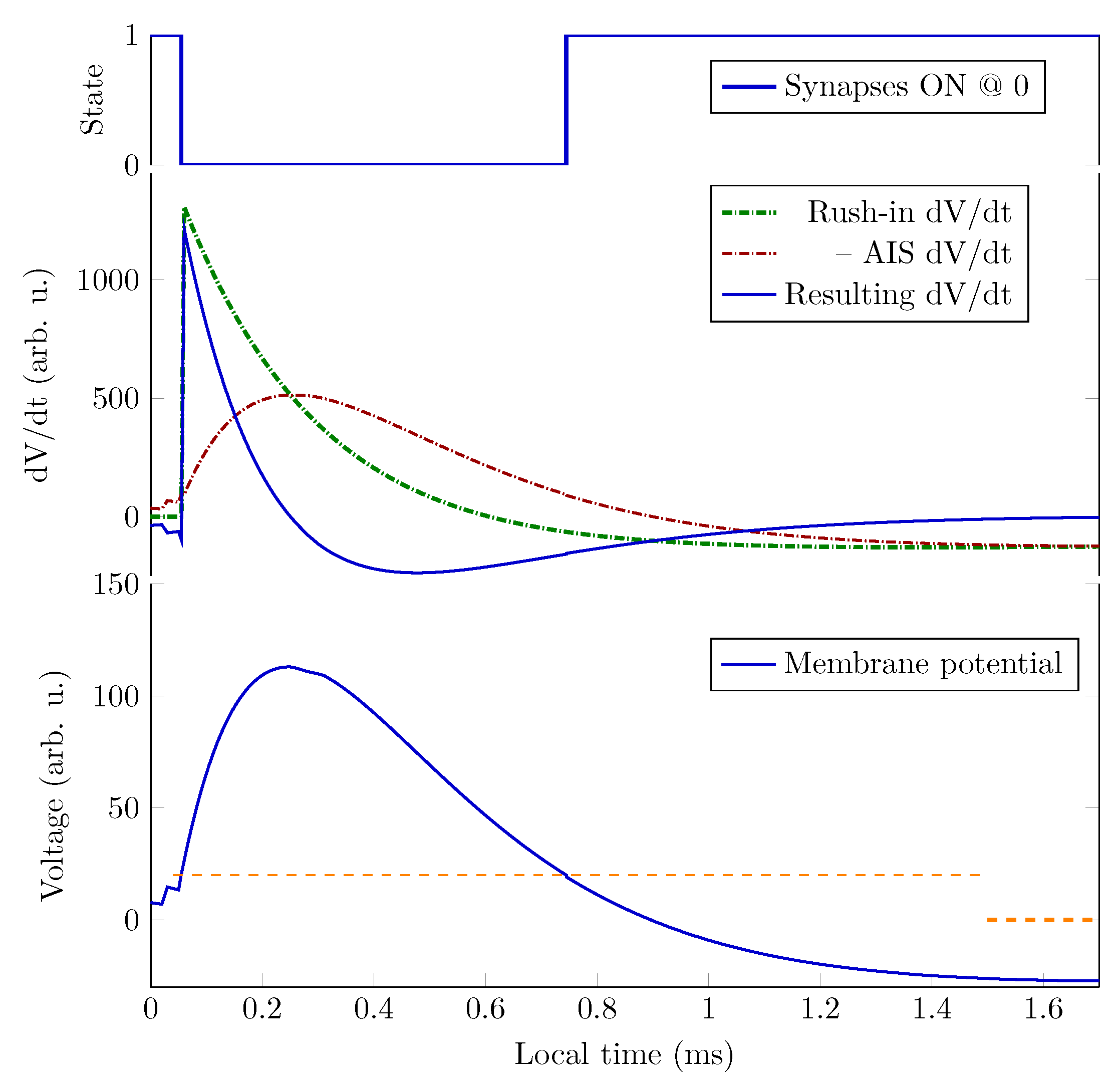
As Figure 3 shows, the non-excitable period of a neuron is shorter than $1msec$, and to integrate the sharp gradient, an integration step about $2\mu sec$ may be needed. Precise time measurement (in the sense that measured by its effect) at this scale can be carried out only by using special hardware devices; the "time slices" the ordinary computers use are at least an order of magnitude larger. By economizing on measuring time, one derives very inaccurate temporal dependencies; see, for example, our Figure 4.

For artificial neurons, the needed time sensitivity should be derived from the technical implementation and strongly depends on the coding/decoding method. In our timing analysis, we check the parameters tha influence the achievable resolution. It was known from the beginning that using von Neumann’s stored-program concept converts the logical dependence on actions into temporal dependence [27]. One must consider that biological computing is inherently parallel, while technical computing is serial (or, at best, parallelized sequentially), breaking down events that co-occur. The fundamental requirement against a correct algorithm is to convert parallelized sequential events into parallel events (with the same time resolution).

1.3. Time

The paper uses different time concepts and emphasizes their differences. The different time concepts are

• biological time that physiologists record when observing biologically meaningful events
• simulated time is a logical time (a biologically faithful time scale) maintained by a user-level scheduler. The simulations of the biological events are scheduled to happen exactly at the true biological time, independent of the computer facilities
• processor time that the processor spends with the simulation task (instruction time and processor speed dependent)
• wall clock time that the programmer records when the computation reaches code parts that simulate biologically meaningful events
• non-payload time that the HW/SW parts of the system spend with needed but not directly task-related activities (system load, task type, and architecture dependent)
• time step (or grid time) a global time step on wall-clock time scale in parallelized computations where different threads/processors wait each for other’s results
• heartbeat time is a per-object and per-stage time step on simulated time scale where values of the simulated variables of a process are calculated
• time resolution on the simulated time scale is the period within which the exact time makes no significant difference (The simulator digitizes the continuous time)
• quasi-biological time assumes a linear dependence between the wall-clock time or the processor time, and the simulated time; used by non-time-aware simulations

Biological time is not related to the complexity of simulating the corresponding events by computing. A biological ’step’ may need a large amount of machine instructions. The non-payload time depends on the workload (which is a very demanding one for neural networks, as the paper emphasizes), and makes the length of the computation quasi-random.

In the text below, the results refer to biological time (sometimes called simulated time). The concept of "grid time" is used in technical computing, where the whole computation (in a technical sense) is suspended, and the gridpoints only communicate: they share their state at the time when the computing was suspended. The "heartbeat time" is actually an integration time step on a biological time scale and does not involve communication. The concept and expression are extensively used in SystemC to distinguish it from "clocking"; it is a less resource-hungry method of timing (independent from the clock-based synchronization) and provides more flexibility for implementing the model.

1.3.1. Time in Technical Computing

In technical computing, an event is an electric signal that denotes the beginning or end of an elementary operation or signals transferring control to another place in the program, or that the program’s control reached a specific instruction in the memory. It has a particular ’wall-clock’ time, a ’processor-time’, and a ’pseudo-biological time’ (in the library and language we use [28], it is called ’simulation time’). The last one (provided that the computer program is accurate and faithfully reproduces neuronal operation) corresponds to biological time, and the paper is about controlling the simulation time of neuronal operation. The other two depend on many factors, and whether they can be uniquely and proportionally mapped to the simulation time is doubtful. Not only can the time of elementary operations be mapped to each other with a factor differing by several orders of magnitude, but they also include the subtleties of computer operation (system calls, Input/Output (I/O) operations, and bus arbitration times) and scheduling computer resources between the simulated biological resources. In addition, the latter two times depend on the type of workload the simulation represents [29,30,31,32,33]. The scaling of computing performance (and, as a consequence, the mapping of computing-related time to biology-related time) is strongly nonlinear.

The notion of time is vital for biological and electronic computing [14]. However, when simulating biological objects by electronic computers, they are not identical, and, what is worse, they are not even proportional. The way computers work [14] destroys even the sequence of events. For this reason, a pseudo-time is used, which we call ’simulated time’. The biological processes are divided into segments of varying sizes. At the characteristic points, the period for the biological process is set and its length is transferred to the scheduler of the engine (important: this scheduler sits on top of the scheduler of the operating system and works independently from it). The information includes a callback function that determines when the activity is to be executed. Many biological processes run simultaneously, and they individually communicate with the scheduler. This way, the scheduler has the information on which biological process wants to use the processor in chronological order.

The scheduler maintains the simulated time as multiples of a ’time resolution’. In this way, the continuous simulated time is mapped to discrete time steps. The time between those discrete steps is considered to be the same. When comparing continuous time values of any kind, a practical need is to define a tolerance (called "time resolution"), a period within which two values are considered equal. A shorter period makes the computation more accurate, but it requires more computing capacity. The time course of the considered biological quantities may also require varying time resolution for the simulation. In this sense, the per-system "grid time" is also a form of time resolution. We use a per-neuron varying "heartbeat time" in the simulator, which is close to the actual time resolution in the simulated biological system, and a (much) smaller technical time resolution used by the simulator’s scheduler.

1.3.2. Time Scales

The basic issue with simulating biology by technological means is that three time scales exist, and they are connected by events only (i.e., non-temporal characteristics of what happens). We have a wall-clock time, that is, how much time passes between the events on the wall-clock; how much processor time is needed to imitate the operating results in the events, and how much textit time the genuine biological system needs to operate between those events. The actual computer processing time is not directly measurable, so a proportionality (implying a homogeneous workload and uniform resource utilization) between the processing and the wall-clock times is usually assumed. After that, the wall-clock time is used as ’the time’ or ’the computing time’, by adding its empirical ratio to the also empirical biological time. The lengths of the computing and the biological operation time periods are not proportional at all. Their ratio depends on several factors, including the technical parameters and architecture of the computing system, as well as the complexity and detail of the computation.

This empirical ratio is an integral quantity (a long-term average) only, it cannot be used directly to align the simulated events. Since biological neurons communicate with each other, and at that given communication time, the equivalent computing time may be different; the time scales of the technical neurons must be aligned by some method, at least approximately. The oldest method (see Algorithm 1) is to use "time slices" (also called "grid time"), i.e., to divide the biological time into slices and to perform simulating calculations only for that slice period in all neurons, then stop. That is, at these synchronization points, all the neuronal computations stop, send the result of their computations to their fellow neurons, and receive similar data.

The ratio of computing time to biological time is called real-time performance (i.e., how closely the two match). To overcome the limitation stemming from the computing workload [29,30,31,32,33], typically, a $1ms$ ’integration time step’ (measured on biological scale) is used. To study biological processes with finer time resolution, one can also use a smaller step time. That step time, however, disproportionately prolongs the overall computation time (slowing down the simulation). Furthermore, see Figure 3, the gradients change steeply; in some phases, needing integration step sizes near $1\mu s$. Figure 4 depicts the effect of the time resolution on the accuracy of deriving a phase diagram.

Natively, computing can only eventually account for the processing time but not control it. It is also hard to find an integration time step which is not waste computing time and still provides sufficiently accurate results.

Algorithm 1 The basic clock-driven algorithm [53], Figure 1

$t\Leftarrow 0$ while  $t<duration$ do     for every neuron do         // State updates         Process incoming spikes         Advance neuron dynamics     end for     for every neuron do         //Propagation of spikes         if $V_M>V_{threshold}$ then            reset neuron            for every connection do                send spike            end for         end if     end for     $t\Leftarrow t+dt$ // Advance to next time by fixed grid time end while

1.3.3. Aligning the Time Scales

The deviation and nonlinearity in the simulation’s wall-clock time and simulated biological time were observed, and various methods to mitigate their effects were introduced. The most straightforward approach is to compare the total simulated time to the total wall-clock time and assume that, on average, a constant factor relates biological time to simulation time. It is, however, not valid for the individual events: they can change their distance and even their order; the time course of the events may differ drastically. The usual (although high-speed) serial bus makes the transfer times nondeterministic [10,14]. In vast technical computing systems, performing all scheduled transfers may require up to dozens of minutes, as shown in Figure 1 of [34]. In other words, the transfer time varies in a quasi-random way between a few nanoseconds and several minutes, so in the worst case, the length of the period of two events with a distance of milliseconds on the biological time scale can amount to minutes on the computing time scale. To avoid practically never-ending computations, "spikes are processed as they come in and are dropped if the receiving process is busy over several delivery cycles" [35]. These are clear signs that, mainly due to the differing operating principles, the vast technical systems cannot handle such an amount and/or density of events that biological simulations need, mainly due to the extensive communication needs. The presently available serial systems do not enable that performance to be reached [31]. "The idea of using the popular shared bus to implement the communication medium is no longer acceptable, mainly due to its high contention." [36].

1.3.4. Time Resolution

The way we perform the simulation is by defining events (such as the beginning or end of computing, receiving an input, etc.) moreover, performing the actions that happen at the same (biological) time. The "same time" in this context means that the simulated times are within a so-called "time resolution". The biological actions are implemented as a kind of callback function that gets called when the corresponding (simulated) time arrives. Choosing a smaller time resolution results in slightly more accurate results at the price of much more computing time. Our experience shows that, given that the time derivative of the rush-in voltage is a very steep function (see Section 4.4), that is made even steeper by adding the Axon Initial Segment (AIS) current-related derivative, should be as low as $2\mu s$ to keep the value of ${\displaystyle \frac{d}{dt}}{V}_M$ around $1mV$ (compare it to the $1ms$ integration step commonly used by neuronal simulators [35]).

1.3.5. Time Stamping

When using timestamping (i.e., attaching the wall-clock times of happening to the events), there are two bad choices. Option one is for neurons to have a (biological) sending-time-ordered input queue and begin processing when all partner neurons have sent their message. (The neurons form a linear chain, but the computing scheduler does not know about that chaining.) That needs a synchrony signal, leading to severe performance loss [31]. Option two is processing the messages as soon as they arrive, enabling one to give feedback to a neuron when processing a message with a timestamp referring to a biologically earlier time, but received physically later. In all cases, it is worth considering if their effect exceeds some tolerance level compared to the last state. Moreover, one shall mitigate the need for communication in this way.

When training an Artificial Neural Network (ANN), one starts showing an input, and the system begins to work. It uses its synaptic weights valid before showing that input. Its initial weights may be randomized or correspond to the previous input data. The system sends correct signals, but a receiver processes a signal only after it is physically delivered (whether or not the message envelope contains a timestamp). It may start to adjust its weight to a state that is not yet defined (in the case of a cyclic operation, to the state in the previous cycle. It is fine in continuously working biological systems, but not when a technical system has just started to work, especially not when upgrading with a new piece of information, leading to ’catastrophic forgetting’). In their operation (essentially an iteration), without synchronization, the actors, in most cases, use wrong input signals, and they surely adjust their weights to false signals initially and with a significant time delay at later stages. Neglecting networks’ temporal behavior, in a lucky case, the system will converge, but painfully slowly. Or not at all.

Synchronization is a must, even in ANNs. Care must be taken when using accelerators, feedback, and recurrent networks. Time matters; furthermore, the computing theory is valid only for linear sequential computing. To provide faster feedback for computing neuronal results faster cannot help. The received feedback delivers the state variables that were valid long ago. In biology, spiking is also a ’look-at-me’ signal: the feedback shall be addressed to that neuron that caused the change (see Hebbian learning). Without considering the spiking time (organizing neuron polling in a software cycle), neurons receive feedback about ’the effect of all fellow neurons, including me’, and adjust all weights of neurons using the same metric. Unlike in biology, the inputs are not distinguished: the same correction is applied to both good and wrong inputs.

1.3.6. Simulating Time

The software we use is a special C++-based library SystemC with a user-level scheduler [28,37]. The primary field of application of the software library is to prepare electronic designs, so some formal elements are to be considered. For using all its features, the complete Reference Guide [37] may be needed for developing the code, but using the well-written core of the packet, no special programming knowledge is necessary, but it is advantageous to study the textbook [28]. The SystemC-specific elements are typically confined to low-level modules. and the user-accessible modules resemble standard C++ modules, although their names and descriptions may reflect their specialties.

When executing the next element of the event queue follows (see Section 3.1.1), the scheduler advances the simulated time to the value of the requested time of action of the actual item. If more than one action is scheduled at the same time, all those actions are performed, in an arbitrary order. At the end of the period, the callback function notifies the biology-imitating process that the requested timing period is over (meaning that the requested computing activity was performed), and the scheduler takes the following item in the queue.

This way, the simulated biological objects work on the same time scale. Through the elapsed time and/or notifying each other, they can cooperate. Although the periods of the simulated time and the period while the computer works out the simulated task are vastly disproportional, the simulation is perfectly timed. The simulated process requests that its phases be scheduled to the biologically correct time, and they are executed at a processor time when the processor has free activity time.

2. Spiking and Information

One of the most eye-catching features (historically) of biological neurons is that they receive and generate intense charge pulses called spikes. It is known from the beginning that "There is, however, another parameter of our neuronal signal. The time interval between the successive impulses can vary" [21]. Although the role of time has been confirmed in several studies, and there is general agreement that time is at the heart of communication within neural systems, there is no consensus on how time is encoded. Even, it is questionable if coding as a metaphor is acceptable for neurons [38].

2.1. Information Coding

We must distinguish "coding" at the perception level and "coding" at the neural communication level. "Information that has been coded [at the perception level] must at some point be decoded also. One suspects, then, that somewhere within the nervous system there is another interface, or boundary, but not necessarily a geometrical surface, where ‘code’ becomes ‘image’” [39]. We use the concept of "coding" at the neuronal level, that is, how the spike pulses convey information. Given that the information is temporally and spatially distributed, moreover, most of the preconditions of the applicability of Shannon’s communication theory [40] are not fulfilled, it is unrealistic to expect a quantitative relation between spikes and the information they deliver.

The information must be coded (and will be converted to a signal after coding), and if so, it must be correspondingly decoded and converted to information. Shannon [41] also warned that this coding/decoding must not be confused with that "the human being acts in some situations like an ideal decoder, this is an experimental and not a mathematical fact". Notice that a human observer sees a signal, instead of the coded information. Up to this point, we can assume that a presynaptic neuron produces information, and the system transfers it to the postsynaptic neuron using an axon. Notice also that Shannon requires cutting a neuron logically to a receiver (the synapses and the membrane) and a transmitter (the AIS) units, in line with what von Neumann introduced, input and output sections.

In neuroscience, "the interpretational gamut implies hundreds, perhaps thousands, of different possible neuronal versions of Shannon’s general communication system" [42]. As we discussed in [6], neuronal communication does not follow Shannon’s model for communication. In this way, some "information loss" is surely incurred. If we consider that the ISI carries information and a neuron takes into consideration in its "computing" only the spikes that arrive within an appropriate time window [10], some information is lost again. Even the result of the computation, a single output spike, may be issued before either of the input spikes was entirely delivered – one more reason why we should revisit the notion of information.

2.2. Spiking

Similarly, definitions such as “Multiple neuromorphic systems use Spiking Neural Networks (SNN) to perform computation in a way that is inspired by concepts learned about the human brain” [43] and “SNNs are artificial networks made up of neurons that fire a pulse, or spike, once the accumulated value of the inputs to the neuron exceeds a threshold” [43] are misleading. That review “looks at how each of these systems solved the challenges of forming packets with spiking information and how these packets are routed within the system”. In other words, the technically needed “servo” mechanism, a well-observable symptom of neural operation, inspired the “idea of spiking networks”. The idea lacks knowledge of information handling and replaces the (in space and time) distributed information content by well-located timestamps in packets, the continuous analog signal transfer by discrete packet delivering, the dedicated wiring of neural systems by bus-centered transfer with arbitration and packet routing, and the continuous biological operating time with a mixture of digital quanta of computer processing plus transferring time. Even the order of timestamps conveyed in spikes (not to mention the information they deliver) is not reminiscent of biology; furthermore, due to the vast need for communication, the overwhelming majority of the generated events must be killed [35] without delivering and processing them to provide a reasonable operating time and to avoid the collapse [44] of the communication system. In the rest of the aspects, the system may provide an excellent imitation of the brain.

In addition to wasting valuable time with contenting for the exclusive use of the single serial bus, utilization of the bit width (and package size) is also inefficient. Temporal precision "encodes the information in the spikes and is estimated to need up to three bits/spike" [45]. The time-unaware timestamping of artificial spikes does not encode temporal precision, given that the message comprises the sending time coordinate of the event instead of the relative time to a local synchrony signal (a base frequency); furthermore, the conduction time is not included in the message. Time stamping misses the biological method of coding information [6]. Moreover, it uses a central clock that is missing from biological systems [46].

2.3. Neuronal Learning

Biological neurons are data-controlled, and they learn autonomously: they adjust their synaptic sensitivity based on the timing relations of the data arriving at their inputs. On the contrary, one must train artificial neurons, typically using the back-propagation method; see [47] and our figures about bus transfer in [10]. During that operation, the program (which works in instruction-driven mode) supervises the learning process, performs computations, and sends its results through the network and the bus in opposite directions. In the figure, the directions of data transmission are opposite in the ’forward’ and ’backward’ directions, whereas time flows in only one direction. One can operate in the ’backward’ direction when the computation in the ’forward’ direction has already terminated (the time windows overlap, and they have no transfer time window between). Furthermore, the above restriction is also valid for the computations inside the layers.

However, the case of ANNs is different. In an ANN, the bus delivers the signals, and the interconnection type and sequence depend on many factors (ranging from the kind of task to the actual inputs). During training ANNs, their feedback complicates the case. The only fixed aspect of timing is that a neuronal input arrives inevitably only after a partner produced it. However, the time ordering of the delivered events may differ from the assumed one. It depends on the technical parameters of delivery rather than the logic that generates them.

2.4. Information Density

As discussed in [6], when sending messages with finite speed, the message comprises temporal and spatial components. The statement applies to both technical and biological computing. In technical computing, the temporal contribution is unintended and unwanted, so it is suppressed as much as possible. In biological computing, the arrival of a spike is only a synchronization signal (in line with Shannon, "if a source can produce only one particular message, its entropy is zero" [40]). The difficulties in deriving experimental conclusions are hard: "These observations on the encoding of naturalistic stimuli cannot be understood by extrapolation from quasi-static experiments, nor do such experiments provide any hint of the timing and counting accuracy that the brain can achieve." [48] In biological systems, evidence shows that more than one bit (some guesses, see [45], ch. 6, suggest 3 bits) is transferred in a spike (modeled as a bit train). When the number of bits in messages can seriously change (and gets significantly higher than one or two bits), the proportionality between the number of spikes and the conveyed information ceases.

An unwanted synergy between computing and neuroscience is the hypothesis that the information transfer and the phenomenon of ’spiking’ (sending short identical pulses) are closely related. A study [48] investigated the connection between spike firing patterns and the visual information they convey. They experienced that "constant-velocity motion produces irregular spike firing patterns, and spike counts typically have a variance comparable to the mean". In statistics, a significant variance indicates that the numbers in a set are far from the mean and from one another. In other words, in the actual case of a constant velocity, there is a very weak (if any) dependence between the number of spikes and the motion, clearly showing that some other parameter of the transferred signal delivers the information. The experimenters noticed this, and they looked for some other "more natural" case: "But more natural, time-dependent input signals yield patterns of spikes that are much more reproducible". Simulating nature-defined encoding is a real challenge, but human-encoding is also made complicated by human-made technical systems. Presumably, in the "much more reproducible" scenario, the number of bits per spike in the analog component is much smaller than in the "less natural" case, so using a wrong merit function for the information meets experimenters’ (false) expectation much better.

The fallacy of selecting a wrong merit function leads directly to the conclusion [49] that "energy efficiency [of neural transfer] falls by well over 90%" (many other similar examples could be cited, but this one shows the mistake explicitly). By defining their measurement method —"We calculated the firing rate of the spiking neuron model" —and measuring "spikes/s"  [48,50] (assuming that the neuron is a repeater and the spike carries on/off information), they draw a false parallel with electronic circuits.

3. Technical Aspects

One can separate the subject of simulating neural networks into two independent segments: what a model is that produces spikes (and what information the spikes convey). and how the system (principally and technically) takes the delivered information into account.

The numerous enormous differences between technical and biological computing make the simulation of neural operation by technical means a real challenge. A fundamental issue is that the biological time of the events is not directly proportional to the computer processing time. Given that the processing time comprises computing time plus transfer time, timestamping cannot provide a solution for time handling. The timestamp records when an event happens in the computing process instead of its biological time. Given that several neurons share the computing resources and the computer’s execution is sequential, the events happening at a biologically identical time will generate time stamps at technically different times. Furthermore, for the same reason, the generated event will be considered again at different times with a (technically random) delay compared to the time of generating those events and to each other. Furthermore, the propagation time through the axons cannot be included. These effects are late consequences of omitting the transfer time in computing science.

3.1. Neural Connectivity

It is typical that several spikes arrive at a neuron, and only one spike is produced (although it branches toward several downstream neurons): “A single neuron may receive inputs from up to 15,000–20,000 neurons and may transmit a signal to 40,000–60,000 other neurons” [51]. “In the terminology of communication theory and information theory, [a neuron] is a multiaccess, partially degraded broadcast channel that performs computations on data received at thousands of input terminals and transmits information to thousands of output terminals by means of a time-continuous version of pulse position. Moreover, [a neuron] engages in an extreme form of network coding; it does not store or forward the information it receives but rather fastidiously computes a certain functional of the union of all its input spike trains which it then conveys to a multiplicity of select recipients" [52].

In small-scale artificial neuronal networks, all neurons in a layer receive input from the neurons of the upstream layer and provide input for the downstream layer. In an extensive system, this method requires an enormous amount of communication actions.

The blue lines inserted into Algorithm 3 illustrate the usually neglected yet necessary and time-consuming actions that were not considered in the algorithm design. When calculating algorithmic time, they are considered as zero-time contributions, but in real computing systems, they can become dominant. In small-scale (toy) systems, they can be neglected. As the system grows, performance saturates, as measurement [33,54] and theory [29,31] have shown.

Algorithm 2 The basic event-driven algorithm with instantaneous synaptic interactions [53], Figure 2

$t\Leftarrow 0$ while queue not empty and $t<duration$ do     Extract event with lowest timing     (=timing t, target i,weight w)     Compute state of neuron i at time t     update state of neuron i (+w)     if $V_M>V_{threshold}$ then         for each connection $i\to j$ do            Insert event in the queue         end for         Reset neuron i     end if end while

Algorithm 3 The basic event-driven algorithm with non-instantaneous synaptic interactions [53], Figure 3

$t\Leftarrow 0$ for every neuron i do     Compute timing of next spike     Insert event in priority queue     Queue handling and I/O end for while queue not empty and $t<duration$ do     Queue handling and I/O     Extract event with lowest timing     (event=timing t, neuron i)     Schedule neuron     Compute state of neuron i at time t     Reset membrane potential     Compute timing of next spike     Insert event in queue     Queue handling and I/O     for every connection $i\to j$ do         Compute state of neuron j at time t         Schedule neuron         Change state with weight w(i,j)         Compute timing of next spike         Insert/change/suppress event in the queue         Queue handling and I/O     end for end while

3.1.1. Queue Handling

Attempts to simulate spiking biological neural networks started early, and different types of simulation strategies and algorithms have been implemented; for an excellent review, see [53]. As experienced, the precision of those simulations sensitively depends on the applied strategies, in particular in cases where plasticity depends on the exact timing of the spikes. It was found that the appropriateness (or applicability) of some method or strategy sensitively depends on the given task. The analysis method can be followed for artificial spiking neural networks, too. The paper discusses the basic algorithms used to compute neural networks (notice that computing the individual neurons according to different models is not detailed).

We detail the calculation algorithm in a single node of the network, as it is the vital component of the correctness of the biological network. Given that, "overall, it appears that the crucial component in general event-driven algorithms is the queue management." [53], we used the highly optimized queue handling of SystemC [28,37]. This way, we use at least one time event and at most one event per neuron in the queue. In most cases, however, servicing one event inserts one or more other events into the queue. An essential difference is that SNNs reduce the possible events to one, while we have a sequence of (non-simultaneous) events per neuron. For SNNs, "Event-driven algorithms implicitly assume that we can calculate the state of a neuron at any given time, i.e., we have an explicit solution of the differential equations". Our approach is distinct: we employ a heartbeat-based calculation method that enables us to determine a neuron’s state at any given (discretized) time.Our method is "spiking" in the sense that a neuron sends a message only when the calculation is complete (thereby minimizing communication). However, it is time-aware (operates on the actual biological time scale) at the cost of increased scheduling complexity. Of course, it can utilize single-shot operating neurons that correspond to step-like changes rather than slow processes.

• the two latter algorithms comprise a deadlock, as all neurons expect the others to compute inputs (or work with values calculated in previous cycles, mixing "this" and "previous" values)
• after processing a spike initiation, the membrane potential is reset, excluding the important role of local neuronal memory (also learning)
• the algorithms are optimized for single-thread processing by applying a single event queue

We must consider the conclusion [53] that "these results support the argument that the speed of neuronal simulations should not be the sole criterion for the evaluation of simulation tools, but must complement an evaluation of their exactness." Following [53], we can assume that enqueue/dequeue operations of events can be performed relatively quickly; however, queue management remains a crucial component in general event-driven algorithms. Moreover, as the number of events in the queue grows, the hit ratio of finding an event in the cache quickly decreases. Given that the memory addresses of neurons found in the queue are "random" for the cache, data locality is not effective anymore, and practically, the processor can access all neuron data after a cache failure. The I/O operations are protected mode instructions, so a single I/O command must be accompanied by context switchings, there and back, with about 20,000 machine instruction offsets [55,56]. This offset is why "artificial intelligence, ...it’s the most disruptive workload from an I/O pattern perspective."1

3.1.2. Limiting Computing Time

One must drop some result/feedback events because of long queuing to provide seemingly higher performance in excessive systems. The feedback the neuron receives provides a logical dependence that the physical implementation of the computing system converts to temporal dependence [14]. The feedback arrives later, so those messages stand at the end of the queue. Because of this, it is highly probable that they "are dropped if the receiving process is busy over several delivery cycles" [35]. In excessive systems, undefined inputs may cause the feedback to become unstable, and the system may ignore (perhaps correct) feedback. Another danger when simulating an asynchronous system on a system that is using at least one single centrally synchronized component introduces a hidden "clock signal" [31], which degrades the system’s computing efficiency by orders of magnitude.

Paper [57] provides an excellent "experimental proof" of the statements above: "Yet the task of training such networks remains a challenging optimization problem. Several related problems arise. Very long training time (several weeks on modern computers, for some problems), the potential for over-fitting (whereby the learned function is too specific to the training data and generalizes poorly to unseen data), and more technically, the vanishing gradient problem". "The immediate effect of activating fewer units is that propagating information through the network will be faster, both at training and test time." The intention to compute feedback faster has its price: As ${\lambda }_s$ increases, the running time decreases, but so does performance." Introducing the spatiotemporal behavior of ANNs improved the efficacy of video analysis significantly [58]. Investigations in the time domain directly confirmed the role of time (mismatching): "The Computer Neural Network (CNN) models are more sensitive to low-frequency channels than high-frequency channels" [59]. The feedback can follow slow changes with less difficulty than faster changes.

3.1.3. Sharing Processing Units

To speed up overall execution, several threads and cores share the task. The different computing times across cores and threads are unrelated to the biological scale, so the programmer divides the biological time into relatively short periods and forcefully stops the simulation in a given thread when the activity up to that biological time has been simulated. That means the threads must wait for each other at the "meeting points" and must mutually inform each other. This is accomplished by sending the relevant calculated result(s) to each other and receiving the results of other computing units as input parameters. This idea is the exact equivalent of the central clocking used by processors. Typically, a $1msec$ "grid time" is used. As we discussed [31], the final result is the same as using a very high-performance processor under the control of a very low-frequency ($1kHz$) central clock. As experienced, the operating characteristics correspond to the theoretical expectations [29,30]. The system can load content into memory in linear time [60] (in this sense, as designed, "can simulate one billion neurons"). However, when those simulated neurons need to communicate, fewer than 80,000 can be operated simultaneously. It means that, at this special workload, the computing efficiency is less than ${10}^{-4}$. It is well understood theoretically [29,30] (the first observation and theoretical description is more than 3 decades old [61]) and it was also experimentally confirmed [32,54] that, for such workloads, only a couple of dozen processors can be used efficiently. It is also known that limiting the number of communication messages, for example, for real-time operation [59], decreases operation quality. In vast systems, collecting the data from all participating processors takes dozens of minutes [34].

After finding the data address, the instruction address must also be set appropriately (it is not certain that all neurons, at all times, execute the same code). Usually, several neurons share a processor core. As [35] estimated, about 10% of the computing capacity is used for administration, provided that once the core is scheduled, all neurons assigned to it compute without needing system-level rescheduling. This means that the relative non-payload contribution can be as good as 10/1000% if all cores are scheduled sequentially, but it can be as wrong as only one payload activity follows the expensive rescheduling operation.

Experience shows that "small differences in spike times can accumulate and lead to severe delays or even cancellation of spikes, depending on the simulation strategy utilized or the temporal resolution within clock-driven strategies used." [53]

3.1.4. Pruning Connections

Communication, anyhow, tragically decreases the efficiency of computation also in large-size neural networks (including brain simulation and ANNs). Grid-time-based computing results in sending and receiving messages regardless of whether a significant change occurs in the neuron’s state. The number of communication actions must be reduced, and the number of epochs (including scheduling) that require non-payload communication must be reduced. The most evident manifestation of biological operation — sending spikes to fellow neurons — inspired the creation of "spiking neural networks". They target reducing messaging by limiting communication to a single message, which is sent by a neuron when it "fires". The issue against the biological application of the idea is the content of the message: the information the spike delivers is the time when the effect of the environment (the fellow neurons) causes the neuron to fire. The time is the ’clock time’ the sender stamps into the message, and the receiver can work out the message based on that time.

In neuroscience, it is known that although a neuron may have several thousand input axons, only about a dozen of them participate in integrating charge (see Eq. (7). Biology also applies pruning during the development of individuals [62,63].

In technical systems, pruning can be applied randomly, based on empirical utilization statistics of the connection line, or using predefined models (such as Large Language Model (LLM)) based on theoretical assumptions on the targeted utilization. The idea of spiking networks is that only the neurons that have collected enough charge send a notification (a spike) to their downstream neurons. This idea reduces the communication traffic considerably, but has ’side effects’ in locality, as discussed. If the spikes carry timing information, the neuron can finish charge integration when sufficient charge has arrived to raise the membrane’s voltage to above the threshold level. This idea assumes that at the time of summing, all input spikes to be considered by a neuron are available as a time-ordered queue, so one can decide when the charge integration shall start and finish. After that time, at a fixed-time delivery offset, the neuron sends a message to its downstream neurons. The arrival time at the downstream neurons is composed of the event time, the delivery time, and the transfer time per connection line.

The time values are on the ’clock time’ scale: the computer prepares the time stamp when executing the operation that caused exceeding the membrane’s threshold. Given that time depends on the thread scheduler (and that up to 1000 neurons per core can be used), in a clock-based algorithm, the neurons send messages (spikes) at approximately the same time offset. When running an event-based algorithm, the non-payload activity is no longer uniform, thereby strongly increasing the dispersion of spiking times and, consequently, reducing the temporal precision of transferring neuronal information.

When imitating biological processes, one needs to consider both the time at which the event can be "seen" in wet neurobiology (the biological time) and the time required for the computer processor to deliver the result corresponding to the biological event (computing time). Computing objects, intended to imitate biological systems, need to be aware of both time scales. As discussed above, in connection with the serial bus, the technical implementation may introduce enormously low payload computing efficiency, and significantly distort the time relations between computing and data delivery times.

The passing of time is measured by counting some periodic events, such as clock periods in computing systems or spiking events in biological systems. In this event-based world, everything that happens between events occurs "at the same time". However, the technical implementation (including the measurement of biological processes) may introduce another unintended granularity. The biological neurons perform analog integration; the technological implementations are prepared to perform "step-wise" digital integration. This step involves (mostly) losing phase information. Furthermore, as detailed in [31], it imposes severe limits on the payload performance for neuronal operations.

Also, an issue is that the artificial neurons work "at the same time" (biological time) and they are scheduled essentially in a random way on the wall-clock time scale. Since the neurons integrate "signals from the past", this method is not suitable for simulating the effects of spikes with a decay time comparable to the length of the grid time. In addition, this grid time is "making all cores likely to send spikes at the same time" and [SpiNNaker]"does not cope well with all the traffic occurring within a short time window within the time step" [35]. This is why the designers of the HW simulator [64] say that the events arrive "more or less" in the same order as they should be. The difference in the timing behavior is also noticed by [35]: "The spike times from the cortical microcircuit model obtained with different simulation engines can only be compared in a statistical sense".

In ANNs, the signals are delivered via a bus, and the interconnection type and sequence depend on many factors (ranging from the kind of task to the actual inputs). During training ANNs, their feedback complicates the case. The only fixed thing in timing is that the neuronal input inevitably arrives only after a partner has produced it (which also takes time). The time ordering of delivered events, however, is not certain: it depends on the technical parameters of delivery, rather than on the logic that generates them. Time stamping cannot help much. There are two bad choices. Option one is that neurons should have a (biological) sending-time-ordered input queue and begin processing only after all partner neurons have sent their message. That needs a synchronous signal and leads to severe performance loss. Option two is that they have a (physical) arrival-time ordered queue, and they are processing the messages as soon as they arrive. This technical solution enables us to give feedback to a neuron that fired later (according to its timestamp), and set a new neuronal variable state, which is a "future state" when processing a message received physically later, but with a timestamp referring to a biologically earlier time. A third, maybe better, option would be to maintain a biological-time ordered queue (that is what SystemC follows), and either in some time slots (much shorter than the commonly used "grid time"), send out output and feedback, individually process the received events, and send back feedback and output immediately. In both cases, it is worth considering whether their effect is significant (exceeds some tolerance level relative to the last state) and, if so, mitigating the need for communication in this way.

In excessive systems, some result/feedback events must be dropped due to long queuing to achieve seemingly higher performance. The logical dependence is that the feedback is computed from the results of the neuron that receives the feedback, the physical implementation of the computing system converts to time dependence [14]. Because of this time sequence, the feedback messages will arrive at the neuron later (even if at the same biological time, according to their time stamp they carry), so they stand at the end of the queue. Because of this, they likely "are dropped if the receiving process is busy over several delivery cycles" [35]. In excessive systems, undefined inputs may establish the feedback, and the system may disregard the (possibly correct) feedback.

An excellent "experimental proof" of the claims above is provided in [57]. With the words of that paper: "Yet the task of training such networks remains a challenging optimization problem. Several related problems arise: very long training time (several weeks on modern computers, for some problems), the potential for over-fitting (whereby the learned function is too specific to the training data and generalizes poorly to unseen data), and more technically, the vanishing gradient problem". "The immediate effect of activating fewer units is that propagating information through the network will be faster, both at training as well as at test time." This effect also means that the computed feedback, perhaps based on undefined inputs, reaches the previous layer’s neurons more quickly. A natural consequence is that (see their Figure 5): "As ${\lambda }_s$ increases, the running time decreases, but so does performance." Similarly, introducing the spatio-temporal behavior of ANNs, even in its simple form, using separated (i.e., not connected in the way proposed in [14]) time and space contributions to describe them, significantly improved the efficacy of video analysis [58].

The role of time (mismatching) is confirmed directly, via time-domain investigations. "The CNN models are more sensitive to low-frequency channels than high-frequency channels" [59]: the feedback can follow slow changes with less difficulty compared to the faster changes.

3.2. Hardware/Software Limitations

The processor time is shared between non-payload tasks, such as the operating system’s tasks [65], including context switching [55,56], as well as scheduling computing tasks and simulated units, and the payload tasks, which involve computing for simulating neuronal activity. For an illustration, we use a flagship project [35]. As published, approximately 10% of the time is spent on non-payload activity. As the calculation in [30] details, the time share and number of cores mean a computing efficacy of ${10}^{-5}$; in other words, out of the ${10}^6$ cores, only 10 can contribute full-value computing performance. This result is in line with the results that (at slightly less demanding workloads) only a few dozen processors (out of several hundreds of thousands) can be effectively used for computation [32,33], similarly to the case of large neural networks [29,54].

Based on theoretical expectations such as "The naïve conversion between Operations Per Second (OPS) and Synaptic Operations Per Second (SOPS) as follows: 1 SOPS ≈ 2 OPS” [66], and the ratio of their operating times ($1ns$ vs $1ms$), it was designed that 1000 neurons share a processor core [35]. That is, in addition to thread scheduling (by the operating system), additional neuron scheduling must also take place (and take time) in the computing thread(s). In this way, much less than $1\mu s$ (on another scale: much less than one thousand machine instructions) can go for calculating the $1ms$ activity of a neuron (a detailed consideration of the required computing cycles is given in [35]). If some neurons cannot complete the required flow of calculations, or if not all simulated neurons have a time slice, and if the computed result cannot be processed, the whole computation in the timeslot is (almost) useless. This is why, according to [35], "Each of these cores also simulates 80 units per core" (out of the designed 1000 units): when reducing the number of required context switchings, the core also has some time to perform payload calculations. The limitation is hard: "As a consequence of the combination of required computation step size and large numbers of inputs, the simulation has to be slowed down compared to real-time. Reducing the number of neurons to be processed on each core, which we presently cannot set to fewer than 80, may contribute to faster simulation" [35].

One of the significant drawbacks of the "grid time" method is that the time resolution (the "sampling rate") cannot be shorter than the "grid time"; the "computing neurons" always send messages at that time, whether they have or not a new state; the event is quantized and, at the end of the "time grid" periods "communication bursts" [44] happen: the achievable performance is severely limited [31]. Especially, the intense communication needed in vast systems can lead to communication collapse [44], limiting the number of collaborating units [35,67], pruning the connections by HW/SW methods [63,68,69] or simply omitting some events to speed up processing [35], apparently.

4. Biological Computing

Biological computing was created by nature without a user’s guide attached, so our basic difficulty is that "engineers want to design systems; neuroscientists want to analyze an existing one they little understand" [70]. We must never forget, especially when experimenting to imitate neuronal learning using recurrence and feedback: "Neurons ensure the directional propagation of signals throughout the nervous system. The functional asymmetry of neurons is supported by cellular compartmentation: the cell body and dendrites (somatodendritic compartment) receive synaptic inputs, and the axon propagates the action potentials that trigger synaptic release toward target cells." [71] We must recall the functional asymmetry and the networked nature (slow, distributed processing) when discussing the biological relevance of a method, such as backpropagation.

A neuron operates in tight cooperation with its environment (the fellow neurons, with outputs distributed in space and time). We must never forget that "the basic structural units of the nervous system are individual neurons" [17], but neurons "are linked together by dynamically changing constellations of synaptic weights" and "cell assemblies are best understood in light of their output product"  [6,72]. A neuron receives multiple inputs at different times (at different offset times from the different upstream neurons) and in different stages. To understand the operation of their assemblies and higher levels, we must provide an accurate description of single-neuron operation.

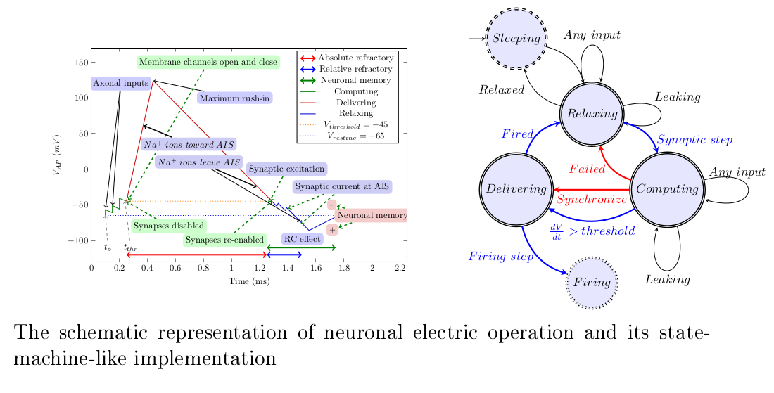
We generalized computing [14], and its in closely integrated communication. Moreover, we extended the idea to biological operations. We abstract the operation as shown in Figure 1, present its mathematical description in Section 4.4, construct its state-diagram-like summary in Figure 2, describe some details of the algorithm in Section 4.5, and present the results of the calculation in Figure 3.

Figure 1. The conceptual graph of the action potential. (Figure 10 from [10]).

Figure 1. The conceptual graph of the action potential. (Figure 10 from [10]).

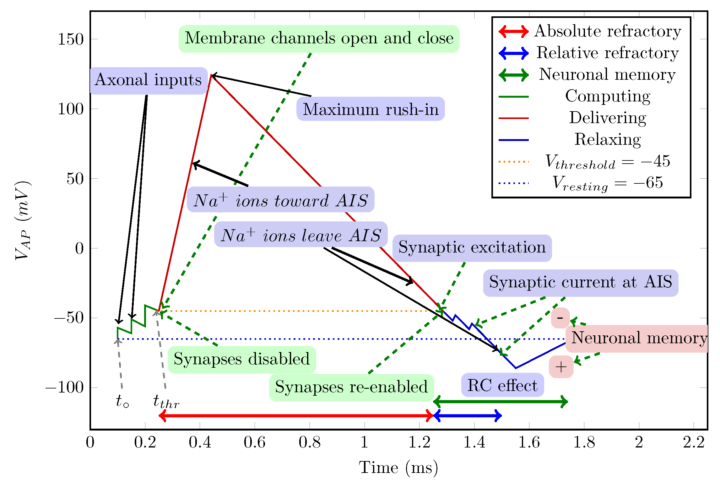
Figure 2. The model of a neuron as an abstract state machine. (Figure 9 from [10]).

Figure 2. The model of a neuron as an abstract state machine. (Figure 9 from [10]).

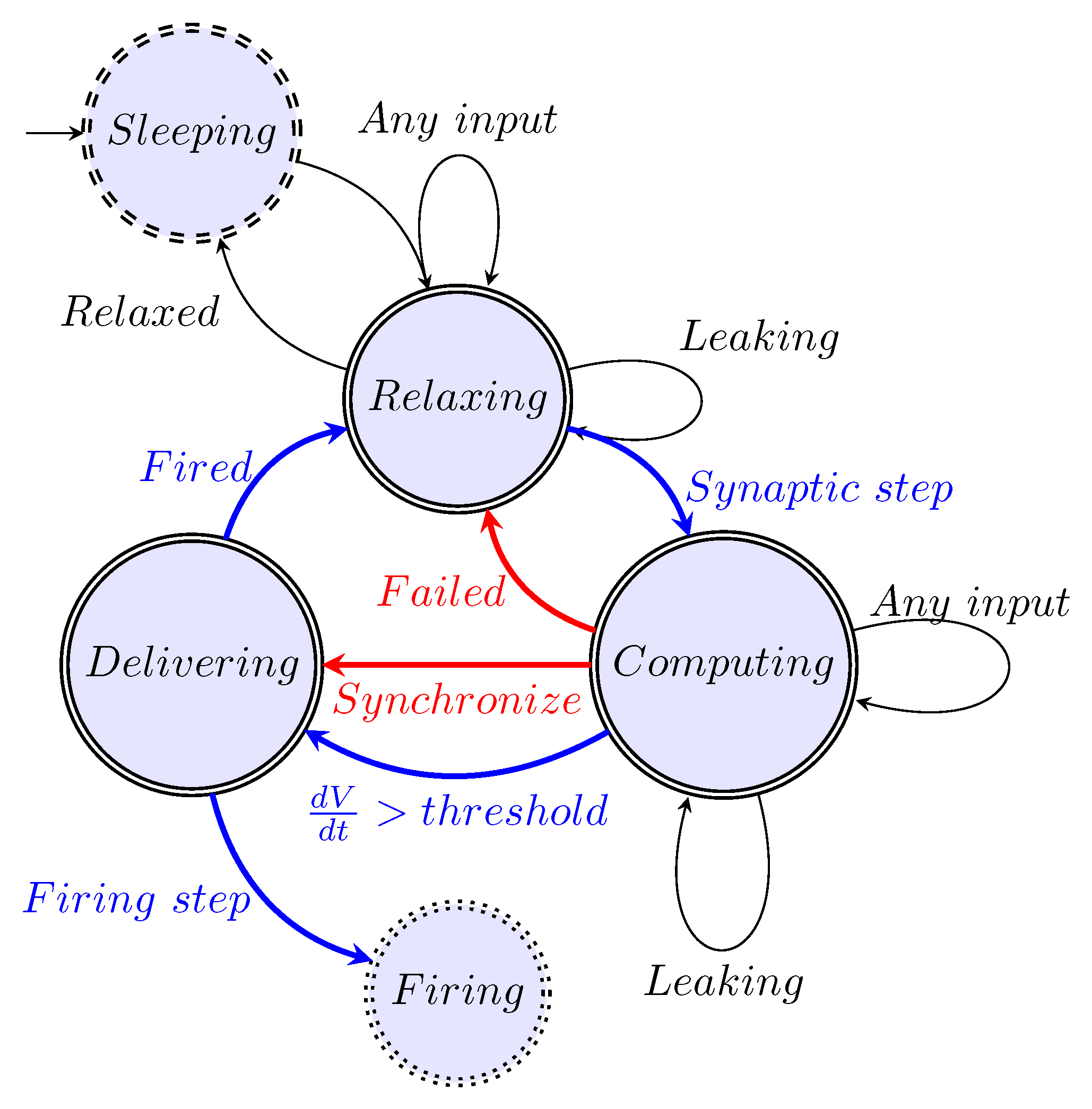
Figure 3. How the physical processes describe membrane’s operation. The rushed-in $N{a}^{+}$ ions instantly increase the membrane’s charge, and then the membrane’s capacity discharges (producing an exponentially decaying voltage derivative). The ions are created at different positions on the membrane, so they take different times to reach the AIS, where the current produces a peak in the voltage derivative.The resulting voltage derivative —the sum of the two derivatives (since the AIS current is outward) —drives the oscillator. Its integration produces the membrane potential.When the membrane potential reaches the threshold voltage, it switches the synaptic currents off or on. (Figure 11 from [10]).

Figure 3. How the physical processes describe membrane’s operation. The rushed-in $N{a}^{+}$ ions instantly increase the membrane’s charge, and then the membrane’s capacity discharges (producing an exponentially decaying voltage derivative). The ions are created at different positions on the membrane, so they take different times to reach the AIS, where the current produces a peak in the voltage derivative.The resulting voltage derivative —the sum of the two derivatives (since the AIS current is outward) —drives the oscillator. Its integration produces the membrane potential.When the membrane potential reaches the threshold voltage, it switches the synaptic currents off or on. (Figure 11 from [10]).

4.1. Conceptual Operation

We describe neuronal operation simultaneously using its conceptual operating graph in Figure 1. We subdivide the neuron’s operation into three stages (green, red, and blue sections of the broken diagram line), in line with the state machine in Figure 2. In the former, we use some biological notions but we omit unnecessary biological details.

Our model incorporates the latest discoveries, including those related to the AIS. The neuron’s operation in the resting state resembles a parallel $RC$ oscillator, but in the transient state it resembles a serial $RC$ oscillator [94]. It has a stage variable (the membrane potential) and a regulatory threshold value. Crossing the membrane’s voltage threshold value upward and downward causes a stage transition from "Computing" to "Delivering" and from "Delivering" to "Relaxing", respectively. In the lack of external current contribution, the length of the period "Delivering" is fixed (defined by physiological parameters), the length of "Computing" depends on the activity of the upstream neurons (furthermore, on the gating due to the membrane’s voltage). Due to the finite speed, we discuss all operations in the neuron’s own "local time".

We consider that the neuron is in a resting ground state [73].Due to an external perturbation, it passes into a transient state and, by releasing the obsolete ions, returns to its resting state. We start in the ’Relaxing’ stage (it is a steady state, with the membrane’s voltage at its resting value). Everything is balanced, and synaptic inputs are enabled. No currents flow (neither input nor output); since all components have the same potential, an output current has no driving force (there is no (significant) "leaking current" [74]).

When the membrane’s voltage decreases below the threshold value, the axonal inputs are reopened, which may mean an instant passing to stage "Computing" again. The current stops only when the charge on the membrane disappears (the driving force terminates), so the current may change continuously, changing the voltage on the circuit’s output. The time of the end of the operation is ill-defined, and so is the value of the membrane’s voltage when the next axonal input arrives. The residual potential acts as a (time-dependent) memory, with about a $msec$ lifetime; see Figure 1. Notice that this is the way nature implements Analog In-Memory Computing (AIMC).

4.2. Stage Machine

Figure 2 illustrates our abstract view of a neuron, in this case, as a "stage machine". The double circles are stages (states with event-defined periods and internal processing) connected by bent arrows representing instant stage transitions. At the same time, at some other abstraction level, we consider them processes that have a temporal course with their event handling. Fundamentally, the system circulates along the blue pathway and maintains its state (described by a single stage variable, the membrane potential) using the black loops. However, sometimes it takes the less common red pathways. It receives its inputs cooperatively (controls the accepted amount of its external inputs from the upstream neurons by gating them by regulating its stage variable). Furthermore, it actively communicates the time of its state change (not its state as assumed in the so-called neural information theory) toward the downstream neurons.

In any stage, a "leaking current" (see Eq. (3)) changing the stage variable is present; the continuous change (the presence of a voltage gradient) is fundamental for a biological computing system. This current is proportional to the stage variable (membrane current); it is not identical to the fixed-size "leaking current" assumed in the Hodgkin-Huxley model [74]. The event that is issued when stage "Computing" ends and "Delivering" begins separates two physically different operating modes: inputting payload signals for computing and inputting "servo" ions for transmitting (signal transmission to fellow neurons begins and happens in parallel with further computation(s)).

The neuron receives its inputs as ’Axonal inputs’. For the first input in the ’Relaxing’ stage, the neuron enters the ’Computing’ stage. The time of this event becomes the base time used for calculating the neuron’s "local time". Notice that to produce the result, the neuron cooperates with upstream neurons (the neuron gates its input currents). One of the upstream neurons opens computing, and the receiving neuron terminates it.

The figure also reveals one of the secrets of the marvelous efficiency of neuronal computing. The dynamic weighting of the synaptic inputs, plus adding the local memory content, happens analog, per synapse, and the summing happens at the jointly used membrane. The synaptic weights are not stored for an extended period. It is more than a brave attempt to accompany (in the sense of technical computing) a storage capacity to this time-dependent weight and a computing capacity to the neuron’s time measurement.

4.2.1. Stage ’Relaxing’

Initially, a neuron is in the ’Relaxing’ stage, which is the ground state of its operation. In this stage, the neuron (re-)opens its synaptic gates. (We also introduce a ’Sleeping’ (or ’Standby’) helper stage, which can be imagined as a low-power mode [75] in the electronic or state maintenance mode of biological computing or "creating the neuron" in biology, a "no payload activity" stage.) The stage transition from "Sleeping" also resets the internal stage variable (the membrane potential) to the value of the resting potential. In biology, a "leaking" background activity takes place: it changes (among others) the stage variable toward the system’s "no activity" value.

The ion channels generating an intense membrane current are closed. However, the membrane’s potential may differ from the resting potential. The membrane voltage plays the role of an accumulator (with a time-dependent content): a non-zero initial value acts as a short-term memory in the subsequent computing cycle. A new computation begins (the neuron passes to the stage ’Computing’) when a new axonal input arrives. Given that the computation is analog, a current flows through the AIS and the result is the length of the period to reach the threshold value. The local time is reset when a new computing cycle begins, but not when eventually the resting potential is reached. Notice that the same stage control variable plays many roles: the input pulse writes a value into the memory (the synaptic inputs generate voltage increment contributions which decay with time, so the different decay times set a per-channel memory value while simultaneously the weighted sum is calculated).

4.2.2. Stage ’Computing’

The neuron receives its inputs as ’Axonal inputs’. For the first input in the "Relaxing" stage, the neuron enters the "Computing" stage. The time of this event is the base time used for calculating the neuron’s "local time". Notice that to produce the result, the neuron cooperates with upstream neurons (the neuron gates its input currents). One of the upstream neurons opens computing, and the receiving neuron terminates it.

The figure also reveals one of the secrets of the marvelous efficiency of neuronal computing. The dynamic weighting of the synaptic inputs, plus adding the local memory content, happens analog, per synapse, and the summing happens at the jointly used membrane. The synaptic weights are not stored for an extended period. It is more than a brave attempt to accompany (in the sense of technical computing) a storage capacity to this time-dependent weight and a computing capacity to the neuron’s time measurement.

While computing, a current flows out from the neuronal condenser, so the arrival time of its neural input charge packets (spikes) matters. All charges arriving when the time window is open increase or decrease the membrane’s potential. The neuron has memory-like states [76] (implemented by different biophysical mechanisms). The computation can be restarted, and its result also depends on the actual neural environment and neuronal sensitivity. Although the operation of neurons can be described when all factors are known, because of the enormous number of factors and their time dependence (including ’random’ spikes), it is much less deterministic (however, not random!) than the technical computation.

The inputs considered in the computation (those arriving within the time window), their weights and arrival times change dynamically between the operations. On the one hand, this change makes it hard to calculate the result; on the other hand, it is accompanied by the learning mechanism, it enables the implementation of higher-order neural functionality, such as redundancy, rehabilitation, intuition, association, etc. Constructing solid electrolytes enables the creation of artificial synapses [77], and many biological facilities in reach, with the perspective of having a thousand times faster neurons, provide facilities for getting closer to the biological operation.

The external signal triggers a stage change and simultaneously contributes to the value of the internal stage variable (membrane voltage). During regular operation, when the stage variable reaches a critical value (the threshold potential), the system generates an event that passes to the "Delivering" stage and "flushes" the collected charge. In that stage, it sends a signal toward the environment (to the other neurons connected to its axon). After that period, it passes to the "Relaxing" stage without resetting the stage variable. From this event on, the "leaking" and the input pulses from the upstream neurons contribute to its stage variable.

4.2.3. Stage ’Delivering’

In this stage, the result is ready: the time between the arrival of the first synaptic input and reaching the membrane’s threshold voltage was already measured. No more input is desirable, so the neuron closes its input synapses. Simultaneously, the neuron starts its ’servo’ mechanism: it opens its ion channels, and an intense ion current starts to charge the membrane. The voltage on the membrane quickly rises, and it takes a short time until its peak voltage is reached. The increased membrane voltage drives an outward current, and the membrane voltage gradually decays. When the voltage drops below the threshold voltage, the neuron re-opens its synaptic inputs and passes to the stage ’Relaxing’: it is ready for the next operation. The signal transmission to downstream neurons happens in parallel with the recent "Delivering" stage and the subsequent "Relaxing" (and maybe "Computing") stages.

The process "Delivering" operates as an independent subsystem ("Firing" ): it happens simultaneously with the process of "Relaxing", which, after some period, usually passes to the next "Computing" stage. The stages "Computing" and "Delivering" mutually block each other, and the I/O operations happen in parallel with them. They have temporal lengths, and they must follow in the well-defined order "Computing"⇒" Delivering"⇒"Relaxing" (a "proper sequencing" [23]). Stage "Delivering" has a fixed period, stage "Computing" has a variable period (depends mainly on the upstream neurons), and the total length of the computing period equals their sum. The (physiologically defined) length of the "Delivering" period limits the neuron’s firing rate; the length of "Computing" is usually much shorter.

4.2.4. Extra Stages

There are two more possible stage transitions from the stage "Computing". First, the stage variable (due to "leaking") may approach its initial value (the resting potential), and the system passes to the " Relaxing" stage; in this case, we consider that the excitation Failed. This happens when the leaking is more intense than the input current pulses (the input firing rate is too low, or a random firing event started the computing). Second, an external pulse [78] “Synchronize” may have the effect of forcing the system (independently from the value of the stage variable) to pass instantly to the "Delivering" stage and, after that, to the "Relaxing" stage. (When several neurons share that input signal, they will go to the "Relaxing" stage simultaneously: they get synchronized, a simple way of synchronizing low-precision asynchronous oscillators.)

4.2.5. Synaptic Control

As discussed, controlling the operation of its synapses is a fundamental aspect of neuronal operation. It is a gating and implements an ’autonomous cooperation’ with the upstream neurons. The neuron’s gating uses a ’downhill method’: while the membrane’s potential is above the axonal arbor’s (at the synaptic terminals), the charges cannot enter the membrane. When the membrane’s voltage exceeds the threshold voltage, the synaptic inputs stop and restart only when the voltage drops below that threshold again; see the top inset of Figure 3. The synaptic gating makes interpreting neural information and entropy [6] at least hard.

4.2.6. Timed Cooperation of Neurons

The length of the axons between the neurons and the conduction velocity of the neural signals entirely define the time of the data transfer (in the millisecond range); all connections are direct. The transferred signal starts the subsequent computation as well (asynchronous mode). "A preconfigured, strongly connected minority of fast-firing neurons form the backbone of brain connectivity and serve as an ever-ready, fast-acting system. However, the full performance of the brain also depends on the activity of very large numbers of weakly connected and slow-firing majority of neurons." [79]

In biology, the inter-neuronal transfer time is much longer than the neuronal processing time. Within the latter, the internal delivery time ("forming a spike") is much longer than the computing (collecting charge from the presynaptic neurons) itself. Omitting the computing time aside from transmission time would be a better approximation than the opposite, as included in the theory. The arguments and the result are temporal; the neural processing is analog and event-driven [39].

Synaptic charges arrive when the time window is open, or artificial charges increase or decrease the membrane’s potential. A neuron has memory-like states [76], see also Figure 1 (implemented by different biophysical mechanisms). The computation can be restarted, and its result also depends on the actual neural environment. When all factors are known, the operation can be described. However, because of the enormous number of factors, their time dependence, the finite size of the neuron’s components, and the finite speed of ions (furthermore, their interaction while traveling on the dendrites), it is much less deterministic (however, not random!) than the technical computation. We learned that it is hard to describe the neuron’s behavior mathematically and to model it electronically. The inputs considered (those arriving within the time window) in the computation, their weights, and arrival times change between the operations, making it hard to calculate the result on the one hand. On the other hand (accompanied by the learning mechanism), it enables the implementation of higher-order neural functionality, such as intuition, association, redundancy, and rehabilitation.

4.3. Classic Stages

We can map our ’modern’ (dynamic) stages to those ’classic’ (static) stages, and we can see why defining the length of the Action Potential is problematic. The effect of slow current affects the apparent boundary between our "Delivering" and "Relaxing" stages. Classical physiology sees the difference and distinguishes ’absolute’ and ’relative’ refractory periods with a smeared boundary between them. Furthermore, it defines the length of the spike with some characteristic point, such as reaching the resting value for the first or second time or reaching the maximum polarization/hyperpolarization. Our derivation of the stages (see Figure 1) defines clear-cut breakpoints between them.

We can define the spike length as the sum of the variable-size length of periods "Computing" and the fixed-size period "Delivering". The "absolute refractory" period is defined as the period when the neuron membrane’s voltage keeps the gates of the synaptic inputs closed (the value of membrane voltage is above their threshold). That period is apparently extended (and interpreted as a "relative refractory" period) by the period when, although the gating is re-enabled. However, the slow current did not yet arrive at the Axon Initial Segment, where it contributes to the measured AP, see Figure 1. Only one refractory period exists, plus the effect of the slow current.

4.4. Mathematics of Spiking 

The so-called equivalent circuit of the neuron is a differentiator-type $RC$ oscillator circuit [10,80,94] as proved by direct neuroanatomical evidence [71,81,82,83,84] (it is erroneously claimed in biophysics that it is an integrator-type oscillator; it is true only for the resting state). The corresponding circuits, their filtering ability, signal forms, and the mathematical form of their description are shown in Table 1. These circuits assume, among others, ’instant interaction’, discrete (non-distributed) electrical components, ideal wires, electrons as charge carriers, constant battery voltage, constant capacitance, constant resistance, and no thermodynamic consequence effects. Neither of them is (strictly) valid for biological circuits. However, these classical circuits are closest to them. The synaptic currents can increase the membrane’s voltage above its threshold, so an intense current starts that suddenly increases the membrane’s voltage to a peak voltage, and then the condenser discharges through the $RC$ circuit. The circuit produces a damped oscillation, and after a longer time, the membrane voltage returns to its resting value. While the membrane’s voltage is above its threshold value, the synaptic inputs are inactive (the analog inputs are gated).

Table 1. RC circuit types.

The RC Integrator	The RC differentiator
$V_{out}^{Integrator}={\displaystyle \frac{1}{RC}}{\int }_0^t{V}_{in}dt$	$V_{out}^{Differentiator}=RC{\displaystyle \frac{d{V}_{in}}{dt}}$
Low Pass Filter	High Pass Filter

Table 1. RC circuit types.

The RC Integrator	The RC differentiator
$V_{out}^{Integrator}={\displaystyle \frac{1}{RC}}{\int }_0^t{V}_{in}dt$	$V_{out}^{Differentiator}=RC{\displaystyle \frac{d{V}_{in}}{dt}}$
Low Pass Filter	High Pass Filter

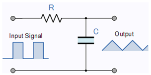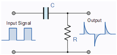Although using an "equivalent circuit" is not perfect for biological circuits, in our model, the neuron is represented as a constant capacity condenser $C_M$ and a constant resistance $R_M$. The charge carriers are slow (typically positive) ions, which are about 50,000 times heavier than electrons (furthermore, they cannot form a "free ion cloud"), while the electrostatic force between the carriers is the same as in the case of electrons. Due to the slow ions, the "instant interaction" model used in the theory of electricity cannot be used. The ions can move only using the “downhill” method (toward decreasing potential), but the potential must be interpreted as the sum of the electric and thermodynamic potentials.

Concerning Figure 1, given that slow ion currents deliver the charge on the membrane’s surface, the charge propagation takes time, and so after the charge-up process, the synaptic inputs reach the output of the circuit about tenths of a millisecond later. Their arrival (the voltage gradients they produce) provides input for the next computing cycle. A potential that resides above the resting potential implements a neuron-level memory.

Although the implementation of a neuronal circuit works with ionic currents with many differences, the operation can align (to some measure) with the instant currents of physical electronics when using current generators of special form. The input currents in a biological circuit is the sum of a large rush-in current through the membrane in an extremely short time and much smaller gated synaptic currents arriving at different times through the synapses. Those currents generate voltage gradients, and the output voltage measured on the output resistor is

$$V_{out}^{Differentiator}=RC{\displaystyle \frac{d{V}_{in}}{dt}}$$

(1)

The figures were generated using $R=0.1G\Omega$ and $C=100pF$. In our ’net’ electric model, it is easy to modify the parameters in steps of solving the differential equation. Note that this solution enables one to take into account the changes in the electric parameters due to mechanical and thermodynamic effects [85,94]. The input voltage gradients are voltage-gated; the logical condition is

$$bool{I}_{Synaptic,i}^{Enabled}=V_{Membrane}^{atposition,i}<V_{threshold}$$

(2)

(the temporal gating, see also Eq.(7) and Figure 3, is implemented through voltage gating). The sum of the input gradients that the currents generate, plus the voltage gradient of the output current generates through the AIS [71,84]. The latter term can be described as

$${\displaystyle \frac{d}{dt}}{V}_{OUT}^{AIS}={\displaystyle \frac{1}{C}}{\displaystyle \frac{V_{internal}-V_{external}}{R}}$$

(3)

That is

$${\displaystyle \frac{d}{dt}}{V}_{in}=\sum {\displaystyle \frac{d}{dt}}{V}_{IN,Gated}^{Component}-{\displaystyle \frac{d}{dt}}{V}_{OUT}^{AIS}$$

(4)

According to Eq.(1), the circuit sums up all derivatives of the gradients, including the one the oscillator generates through the AIS. So a composite signal appears at the output resistor (not to mention that the synaptic inputs are gated: they are not effective during the stage ’Delivering’). This differentiator circuit natively produces positive and negative voltages for rising and falling edges of the input voltages. For the resting state, the ’no gradient’ case, of course, produces ’no output voltage’. According to Eq.(3), the voltage drop on the AIS is proportional to the voltage above the resting state, so there is no ’leakage current’ in the resting state; with far-reaching biological consequences [94]. In the transient state, the integrating effect of the condenser forms the output signal to behave as ’polarized’ and ’hyperpolarized’ parts of the neural signal (see the bottom inset in Figure 3), without needing to hypothesize any current in the opposite direction. It is a native feature of the correct sequential circuit; the parallel circuit cannot produce similar behavior and requires ad hoc non-physical hypotheses.

The input currents (although due to slightly differing physical reasons for the different current types) are usually described by an analytic form

$$I_{in}=I_o\ast \left(1-exp(-{\displaystyle \frac{1}{\alpha }}\ast t)\right)\ast exp\left(-{\displaystyle \frac{1}{\beta }}\ast t\right)$$

(5)

where $I_o$ is a current amplitude per input, $\alpha$ and $\beta$ are timing constants for current in- and outflow for the given contributing current, respectively. They are (due to geometrical reasons) approximately similar for the synaptic inputs and differ from the constants valid for the rush-in current. The corresponding voltage derivative is

$${\displaystyle \frac{d{V}_{in}}{dt}}={\displaystyle \frac{I_o}{C}}\ast \left({\displaystyle \frac{1}{\alpha }}\ast exp\left(-{\displaystyle \frac{1}{\alpha }}\ast t-{\displaystyle \frac{1}{\beta }}\ast t\right)-{\displaystyle \frac{1}{\beta }}\ast exp\left(-{\displaystyle \frac{1}{\beta }}\ast t)\ast exp(1-exp(-{\displaystyle \frac{1}{\alpha }}\ast t)\right)\right)$$

(6)

To implement such an analog circuit with a conventional electronic circuit, voltage-gated current injectors (with time constants of around $1ms$) are needed. Notice that the currents have a range of validity of interpretation as described. The input (synaptic) currents are interpreted only in "Computing"; the rush-in current flows only from the beginning of "Delivering" while the outward current (see Eq.(3)) is persistent but depends on the membrane’s potential.

In the simplest case, the resulting voltage derivative comprises only the rush-in contribution described by Eq (6) and the AIS contribution described by Eq. (3). The gating implements a dynamically changing temporal window and dynamically changing synaptic weights. The appearance of the first arriving synaptic gradient starts the “Computing” stage. The appearance of the rush-in gradient starts the “Delivering” stage. The charge collected in that temporal window is

$$Q\left(t\right)={\int }_{t_{0,i}}^{t_{thr}}dt\underset{t_{0,i}\le t\le t_{thr}}{\underbrace{\sum _i}}{I}_{syn,i}\left(t\right)$$

(7)

The total charge is integrated in a mathematically entirely unusual way: the upper limit depends on the result. Notice that artificial neural networks (including "spiking neural networks") entirely overlook this point: Notice that artificial neural networks (including "spiking neural networks") entirely overlook this point: integration is continuous (all summands are used), and the result reduces to a logical variable. Also, it is not considered that the AIS current decreases the membrane’s voltage and charge between incoming spikes.

This omission also has implications for the algorithm. The only operation that a neuron can perform is that unique integration. It is implemented in biology by gating the inputs to the computing units, as shown in Eq.(2). In the "Computing" stage, synaptic inputs are open; in the "Delivering" stage, they are closed (the inputs are ineffective). It produces multiple outputs (in the sense that the signal may branch along its path) in the form of a signal with a temporal course. Although it has many (several thousand) inputs, a neuron uses only about a dozen of them in a single computing operation, appropriately and dynamically weighting and gating its inputs [79].

The result of the computation is the reciprocal of the weighted sum, and it is represented by the time when a spike is sent out (when that charge on the membrane’s fixed capacity leads to reaching the threshold). Any foreign (artificial, such as clamping) current influences the rate of charge collection and, therefore, the $t_{thr}$ value; its time course also contributes to the overall gradient. The neuron (through the integration time window) selects which ones out of its upstream neurons can contribute to the result. The individual contributions are a bargain between the sender and the receiver: the neuron decides when a contributing current terminates, but an upstream neuron decides when it begins. The beginning of the time window $t_o$ is set by the arrival of a spike from one of the upstream neurons, and it is closed by the neuron when the charge integration results in a voltage exceeding the threshold. The computation (a weighted summation) is performed on the fly, excluding the obsolete operands. (The idea of AIMC [86] almost precisely reproduces the charge summation except for its timing.)

Figure 3 (resulted by our simulator [80]) shows how the described physical processes control a neuron’s operation. In the middle inset, when the membrane’s surface potential, see Eq.(1), increases above its threshold potential due to three step-like excitations opens the rush-in ion channels instantly (more details in [10,80]), and creates an exponentially decreasing, step-like voltage derivative that charges up the membrane. The step-like imitated synaptic inputs resemble the real ones: the synaptic inputs produce smaller, rush-in-resemblant (see Figure 10 in  [87]), voltage gradient contributions. When integrated as Eq. (1) describes the resulting voltage gradient that produces the Action Potential (AP) shown in the lower inset. Crossing the threshold level controls the gating signal. as shown in the top inset.

Notice how nature implemented "in-memory computing" by weighted parallel analog summing. The idea of AIMC [86] quite precisely reproduced the idea, except that it uses a "time of programming", instead of the "time of arrival" the biological system uses. The "time of programming" depends on technical transfer characteristics. In general, that time is measured on the scale of computing time rather than simulated time.

Notice nature’s principles of reducing operands and noise: the less important inputs are omitted by timing. The rest of the signals are integrated over time. The price paid is a straightforward computing operation: the processor can perform only one type of operation. Its arguments, result, and neuronal-level memory are all time-dependent. Furthermore, the operation excludes all but (typically) a dozen neurons from the game. It is not necessarily the case that the same operands, having the same dynamic weights, are included in consecutive operations. It establishes a chaotic-like operation [88] at the level of the operation of neuronal assemblies [48,72,89], but also enables learning, association, rehabilitation, and similar functionalities. Since the signal’s shape is identical, integrating them in time means multiplying them by a weight (depending non-linearly on time), and the deviation from the steady-state potential represents a (time-dependent) memory. The significant operations, the dynamic weighting, and the dynamic summing are performed strictly in parallel. There are attempts to use analog or digital accelerators (see [86,90]), but they work at the expense of degrading either the precision or the computing efficiency. Essentially, this is why, from the point of view of technical computation, “we are between about 7 and 9 orders of magnitude removed from the efficiency of mammalian cortex” [35].

4.5. Algorithm for the Operation

As can be concluded by from our Figure 1 and Figure 2, the computation and the event control heavily depend on the stage of the operation, although the underlying logic is the same. When the calculation occurs at the ’heartbeat’ times, the system updates the neuron’s state and changes its stage if needed.

Algorithm 4 The main computation

//Calculate stage-dependent contributions if Stage "Relaxing" then     if ($RelaxingStopped$) then         ${{\displaystyle \frac{dV}{dt}}}_{Rushin}\Leftarrow 0;$     else          ${{\displaystyle \frac{dV}{dt}}}_{Rushin}\Leftarrow Eq.\left(6\right)$ for rushin current at time t     end if end if if Stage "Computing" then     ${{\displaystyle \frac{dV}{dt}}}_{Rushin}\Leftarrow 0;$     ${{\displaystyle \frac{dV}{dt}}}_{Input}\Leftarrow Eq.\left(6\right)$ for input currents at time t end if if Stage "Delivering" then     $SynapsesEnabled\Leftarrow (V_{Membrane}<V_{Threshold})$     ${{\displaystyle \frac{dV}{dt}}}_{Rushin}\Leftarrow Eq.\left(6\right)$ for rushin current at time t     ${{\displaystyle \frac{dV}{dt}}}_{Input}\Leftarrow Eq.\left(6\right)$ for input currents at time t; according to Eq.(4) end if ${{\displaystyle \frac{dV}{dt}}}_{Resulting}\Leftarrow Eq.\left(4\right)$ ${{\displaystyle \frac{dV}{dt}}}_{AIS}\Leftarrow Eq.\left(3\right)$ for the output current at time t $V_{Membrane}\Leftarrow +{{\displaystyle \frac{dV}{dt}}}_{Resulting}\ast dt$ from Eq.(1) Adjust heartbeat time and set new time

Algorithm 5 The heartbeat computation

if Stage "Relaxing" then     if ReceivedSynapticInput then         Send ’BeginComputing’     end if     if ${\left({\displaystyle \frac{dV}{dt}}\right)}_{Membrane}<0$ then         if $abs\left(V_{Membrane}\right)<Allowed$ then            $V_{Membrane}\Leftarrow 0$            $RelaxingStopped\Leftarrow true$         end if     end if end if if Stage "Computing" then     if $V_{Membrane}<0$ then         Send ’Failed’     end if else     if $V_{Membrane}>=V_{Threshold}$ then         $SynapsesEnabled\leftarrow false$         Send ’DeliveringBegin’     end if end if if Stage "Delivering" then     if $V_{Membrane}<V_{Threshold}$ then         $RelaxingStopped\Leftarrow true$         $SynapsesEnabled\leftarrow true$         Start ’RelaxingBegin’     end if end if Do main computing in Algorithm (4) Send new heartbeat

4.6. Operating Diagrams

Figure 3 (produced by the simulator) shows how the described physical processes control a neuron’s operation. In the middle inset, when the membrane’s surface potential increases above its threshold potential due to three step-like excitations opening the ion channels, $N{a}^{+}$ ions rush in instantly and create an exponentially decreasing, step-like voltage derivative that charges up the membrane. The step-like imitated synaptic inputs are reminiscent of the real ones: the incoming Post-Synaptic Potential (PSP)s produce smaller, rush-in-resemblant, voltage gradient contributions. The charge creates a thin surface layer current that can flow out through the AIS. This outward current is negative and proportional to the membrane potential above its resting potential. In the beginning, the rushed-in current (and correspondingly, its potential gradient contribution) is much higher than the current flowing out through the AIS, so for a while, the membrane’s potential (and so: the AIS current) grows. When they get equal, the AP reaches its top potential value. Later, the rush-in current gets exhausted, and its potential-generating power drops below that of the AIS current; the resulting potential gradient changes its sign, and the membrane potential starts to decrease.

In the previous period, the rush-in charge was stored on the membrane. Now, when the potential gradient reverses, the driving force starts to decrease the charge in the layer on the membrane, which, by definition, means a reversed current; without foreign ionic current through the AIS. This is a fundamental difference between the static picture that Hodgkin and Huxley hypothesized [74] and biology uses, and the dynamic one that describes its behavior. The microscopes’ resolution enabled one to discover AIS only two decades after their time; their structure and operation could be studied only three more decades later [71]. In the past two decades, it has not been built into the theory of neuronal circuits. The correct equivalent electric circuit of a neuron is a serial oscillator in the transient state, and a parallel oscillator in the resting state (see [10,80]), and its output voltage in the transient state is defined dynamically by its voltage gradients instead of static currents (as physiology erroneously assumes). In the static picture, the oscillator is only an epizodist, while in the time-aware (dynamic) picture, it is a star.

Notice also that only the resulting ${\displaystyle \frac{dV}{dt}}$ Action Potential Time Derivative (APTD) disappears with time. Its two terms are connected through the membrane potential. As long as the membrane’s potential is above the resting value, a current of variable size and sign will flow, and the output and input currents are not necessarily equal: the capacitive current changes the game’s rules.

Figure 4 (resulting from our simulator [80]) shows the phase diagram between the membrane’s potential and its voltage gradient, compared to the measured diagram from [91], Figure 2.d. In this parametric figure, the time parameter is derived from both experimental and simulated data. The sampling base distance is not equidistant in time. On the blue experimental line, the measurement times are marked by joint broken-line segments. On the red theoretical diagram line, the marks indicate the points where the simulated value was calculated (the time is adjusted to the actual gradient). As discussed, the improper measurement periods act as averaging over improperly selected time intervals. On the right side of the figure, the broken line, although rough, properly follows the time course of the theoretical diagram line. The measurement periods are slightly above the optimal, around 0.1 milliseconds. However, this is not the case in the middle of the figure. Here, the time distance of the sampling points is about $2\mu s$, and the rush-in of the $N{a}^{+}$ ions causes a drastically different gradient value. This fine time resolution enables us to track the effect, whereas the "long" measurement resolution period yields an improper average and masks the effect that drives neuronal operation. The effect clearly demonstrates the need for a gradient-aware algorithm and an integration step; furthermore, it shows that voltage gradients control neuronal operation.

The top inset shows how the membrane potential controls the synaptic inputs. Given the ions from the neuronal arbor [92,93] can pass to the membrane using the ’downhill’ method, but they cannot do so if the membrane’s potential is above the threshold. The upper diagram line shows how this gating changes in time’s function.

Figure 4. The diagram describing the Action Potential in the $Vvs{\displaystyle \frac{dV}{dt}}$ phase diagram. A parametric figure showing the correspondence between the membrane’s potential, see Eq. (1) and its gradient, see Eq. (3). The theory’s diagram line perfectly describes the experimental data (see [91], Figure 2.d) where the distance between the sampling data points is adequate.

Figure 4. The diagram describing the Action Potential in the $Vvs{\displaystyle \frac{dV}{dt}}$ phase diagram. A parametric figure showing the correspondence between the membrane’s potential, see Eq. (1) and its gradient, see Eq. (3). The theory’s diagram line perfectly describes the experimental data (see [91], Figure 2.d) where the distance between the sampling data points is adequate.

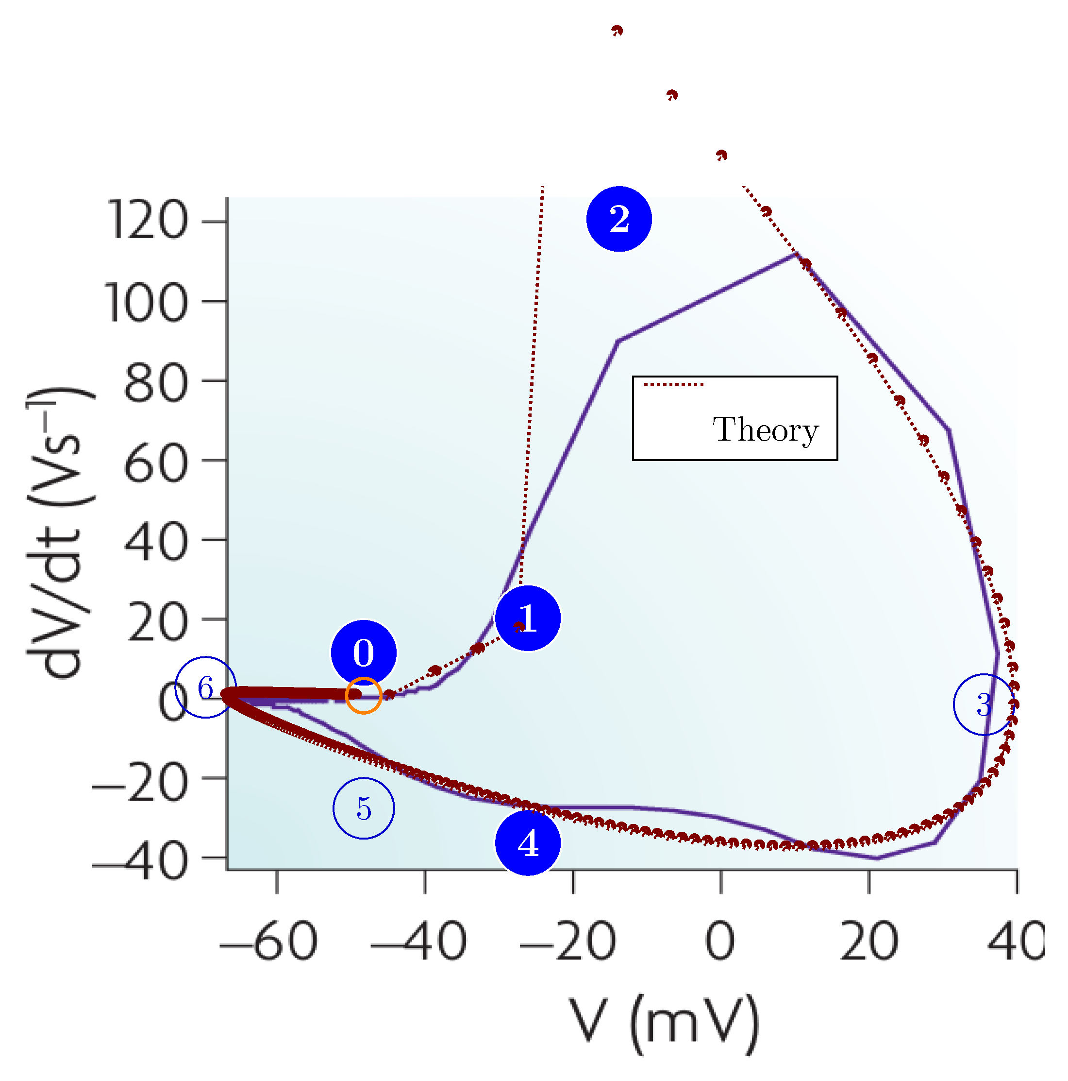
4.7. Implications of the Model and the Algorithm

All former models and simulators lack a proper physical basis.As Hodgkin and Huxley (HH) correctly noted, the physical picture they had tentatively in mind when they attempted to give meaning to their mathematical equations describing their observations was wrong. Their followers never attempted to validate or replace the mechanisms they hypothesized; only different mathematical formulas were suggested to have fewer (or just another) contradictions with the observations. No other simulator works with a correct physical background. They parametrize some mathematical functions, but they lack the physical processes underlying them. Neither of those parameters can be described from the first principles/ scientific laws.

The concept of scalability has different readings when speaking about different times and different compositions of processing and communication times. The net computing activity grows linearly with the number of simulated neurons. SystemC is based on single-thread, user-level scheduling (although there are extensions for taking advantage of operating system (OS)-level multi-threading). This way it avoids using time-wasting I/O instructions, system-level processor and thread scheduling.

A neuron operates in tight cooperation with its environment (the fellow neurons, with outputs distributed in space and time). We must never forget that "the basic structural units of the nervous system are individual neurons" [17], but neurons "are linked together by dynamically changing constellations of synaptic weights" and "cell assemblies are best understood in light of their output product" [6,72]. To understand the operation of their assemblies and higher levels, we must provide an accurate description of single-neuron operation. Unlike the former models and algorithms, Eq.(7) expresses this observation, called ’synaptic plasticity’. Neurons process information autonomously, but in cooperation with their environment. They receive multiple inputs at different offset times from different upstream neurons at different stages. The earliest input defines the beginning of the time window, and the neuron (based on the result of the analog integration) defines the end of the time window. The time window defines the synaptic weight used in the operation for received synaptic inputs. Not only the synaptic weights but also the contributors may change from cycle to cycle. Unlike any former model or mathematical formula, our model natively explains synaptic plasticity, and the algorithm can implement it.

Learning is a very complex mechanism, and nature uses time windows of different widths (ranging from fractions of a millisecond to minutes) to implement it. Although not fully discussed, some hints are given by the author in [10] (and will be given in forthcoming papers). The paper did not intend to define such features. The present model deals with the elementary operation of a single neuron, although it mentions one possible implementation of memory.

"Synaptic interactions" is a concept that is the consequence of the concept of ’instant interaction’. Synaptic inputs, which provide parallel contributions in biology, and are processed by analog parallel computing units, can only be handled by sequential processing in technical computing. This way, technical implementations unavoidably work with values of different time arguments when handling different inputs. To avoid that, the implementation must "freeze" the time. In our perfectly timed implementation, we use a simulated biological time scale. We use "intended" time, and truly simultaneous events that are independent from the technical implementation, actual workload, and so on. In non-perfect implementations, either a linear mapping is tacitly assumed or a timestamp (containing a wall-clock time or processor-clock time) attempts to "freeze" the time, always comprising distortions from foreign computing activities. This means that when imitating biological activity by processing sequentialized parallel input, the ’instant interaction’ algorithm must somehow correct for the (non-biological) effect. A fictitious method must consider that the other inputs somehow (that "will happen at the same time, but not yet processed") distorts the result. Synapses are one-way objects; their interactions are parallel in biology, and some artefact had to be created to simulate their sequential imitation.

5. Summary

By using a programming technology developed for designing tightly synchronized high-speed electronic circuits, we provided an exact implementation of the physically (including the time courses of the processes) correct model of a biological neuron. The gradient-driven operation of neurons, the multitude and complexity of the physical processes needed for the development of a cross-disciplinary physical model (up to now, only the ’net electric’ part is elaborated), which is based on first principles of science, uses well-established mathematical differential equations (without any empirical functions). The algorithm based on that technology enables one to follow the physical processes in the background with arbitrary precision. Their combination faithfully reproduces the biological operation of a single neuron, opening the way to modeling the temporal behavior of cooperating neurons.

We delivered a simplified ’net electrical’ model for neuronal operation and contrasted it to the almost exclusively used ’net electrical’ Hodgkin-Huxley model. We fixed some fundamental mistakes (the oscillator type, the assumed ’instant electric interaction’, the lack of ’driving force’, and the neglect of bio-electric generation of voltages) in the latter model. We provided a solid, correct physical background for it. We provided a mathematical description that is almost identical to the one developed in classical electricity for describing a ’serial $RC$ oscillator circuit’. However, nature unusually uses the circuit (instantly injected charges, slow ion currents, gated analog inputs, spatially and temporally distributed information, slow and tuned networking), and its technical imitation requires extremely high precision. Given that the development of computing technology introduced solutions (e.g., system calls, time slicing, caching, interrupts, operating system schedulers, thread scheduling and synchronization, I/O operations, queuing) that broke the simple linear execution of machine instructions; a faithful temporal implementation of biological processes is not possible with the expected temporal precision. For that goal, we introduced a technology that was developed for the electronic design industry, where the timing requirements and especially the correct time ordering is of extreme importance. The operating cycle of a neuron involves different physical mechanisms, so we divided the description and the mathematical handling into stages correspondingly. The fact that biology uses "slow currents" forced us to imitate the real features of a "slow current" by using a special distribution of "fast current". Fortunately, the parameters of that distribution could be derived from physiological measurements. Since biology uses analog data collection with gated inputs and enforces a "proper sequencing" (von Neumann) of the stages, furthermore, for reproducing the precise timing of the biologically meaningful events, a unique computational algorithm had to be developed. By providing a neuron with reproducible and parametrizable behavior, a new research facility is released that enables the study of, among others, learning, association, and rehabilitation; furthermore, studying networked behavior, imitating diseases by changing the electric (and other) parameters (see [94]) for precise simulation.

References

- Human Brain Project. New HBP-book: A user’s guide to the tools of digital neuroscience, 2023.
- Bell, G.; Bailey, D.H.; Dongarra, J.; Karp, A.H.; Walsh, K. A look back on 30 years of the Gordon Bell Prize. The International Journal of High Performance Computing Applications 2017, 31, 469–484.
- Ngai, J. BRAIN @ 10: A decade of innovation. Neuron 2024, 112. [CrossRef]
- Schrödinger, E., Is life based on the laws of physics? In What is Life?: With Mind and Matter and Autobiographical Sketches; Cambridge University Press: Canto, 1992; p. 76–85.
- Végh, J. The non-ordinary laws of physics describing life. European Biophysical Journal 2025, 1, in review.
- Végh, J.; Berki, Á.J. Towards generalizing the information theory for neural communication. Entropy 2022, 24, 1086–. [CrossRef]
- Drukarch, B.; Wilhelmus, M. Thinking about the nerve impulse: A critical analysis of the electricity-centered conception of nerve excitability. Progress in Neurobiology 2018, 169, 172–185. [CrossRef]
- Drukarch, B.; Wilhelmus, M. Thinking about the action potential: the nerve signal as a window to the physical principles guiding neuronal excitability. Frontiers in Cellular Neuroscience 2023, 17. [CrossRef]
- Feynman, R.P. Feynman Lectures on Computation; CRC Press, 2018.
- Végh, J. On Implementing Technomorph Biology for Inefficient Computing. Applied Sciences 2025, 15. [CrossRef]
- von Neumann, John. The Computer and the Brain; New Haven, Yale University Press, 1958.
- Abbott, L.; Sejnowski, T.J. Neural Codes and Distributed Representations; Cambridge, MA: MIT Press, 1999.
- Chu, D.; Prokopenko, M.; Ray, J.C. Computation by natural systems. Interface Focus 2018, 8. Accessed: 2025-03-20, . [CrossRef]
- Végh, J. Revising the Classic Computing Paradigm and Its Technological Implementations. Informatics 2021, 8. [CrossRef]
- Mehonic, A.; Kenyon, A.J. Brain-inspired computing needs a master plan. Nature 2022, 604, 255–260. [CrossRef]
- Markovic, D.; Mizrahi, A.; Querlioz, D.; Grollier, J. Physics for neuromorphic computing. Nature Reviews Physics 2020, 2, 499–510.
- Johnston, D.; Wu, S.M.S. Foundations of Cellular Neurophysiology; Massachusetts Institute of Technology: Cambridge, Massachusetts and London, England, 1995.
- Kandel, E.R.; Schwartz, J.H.; Jessell, T.M.; Siegelbaum, S.A.; Hudspeth, A.J. Principles of Neural Science, 5 ed.; The McGraw-Hill Medical: New York Chicago etc., 2013.
- Hebb, D. The Organization of Behavior; New York: Wiley and Sons, 1949.
- Caporale, N.; Dan, Y. Spike Timing–Dependent Plasticity: A Hebbian Learning Rule. Annual Review of Neuroscience 2008, 31, 25–46. PMID: 18275283, . [CrossRef]
- MacKay, D.M.; McCulloch, W.S. The limiting information capacity of a neuronal link. The bulletin of mathematical biophysics 1952, 14, 127–135.
- Sejnowski, J.T. The Computer and the Brain Revisited. Annals Hist Comput 1989, pp. 197–201.
- von Neumann, J. First draft of a report on the EDVAC. IEEE Annals of the History of Computing 1993, 15, 27–75. [CrossRef]
- Nature. Documentary follows implosion of billion-euro brain project. Nature 2020, 588, 215–216. [CrossRef]
- Human Brain Project. A closer look at scientific advances, 2023.
- Nemenman, I.; Lewen, G.D.; Bialek, W.; de Ruyter van Steveninck, R.R. Neural Coding of Natural Stimuli: Information at Sub-Millisecond Resolution. PLOS Computational Biology 2008, 4, 1–12. [CrossRef]
- Backus, J. Can Programming Languages Be liberated from the von Neumann Style? A Functional Style and its Algebra of Programs. Communications of the ACM 1978, 21, 613–641.
- Black, C.D.; Donovan, J.; Bunton, B.; Keist, A. SystemC: From the Ground Up, second ed.; Springer: New York, 2010.
- Végh, J. Which scaling rule applies to Artificial Neural Networks. Neural Computing and Applications 2021, 33, 16847–16864. [CrossRef]
- Végh, J. Finally, how many efficiencies the supercomputers have? The Journal of Supercomputing 2020, 76, 9430–9455, regularly updated at https://arxiv.org/abs/2001.01266.
- Végh, J. How Amdahl’s Law limits performance of large artificial neural networks. Brain Informatics 2019, 6, 1–11. [CrossRef]
- D’Angelo, G.; Rampone, S. Towards a HPC-oriented parallel implementation of a learning algorithm for bioinformatics applications. BMC Bioinformatics 2014, 15.
- D’Angelo, G.; Palmieri, F. Network traffic classification using deep convolutional recurrent autoencoder neural networks for spatial–temporal features extraction. Journal of Network and Computer Applications 2021, 173, 102890. [CrossRef]
- hpcwire.com. TOP500: Exascale Is Officially Here with Debut of Frontier. https://www.hpcwire.com/2022/05/30/top500-exascale-is-officially-here-with-debut-of-frontier/ , 2022. Accessed: 2023-09-10.
- van Albada, S.J.; Rowley, A.G.; Senk, J.; Hopkins, M.; Schmidt, M.; Stokes, A.B.; Lester, D.R.; Diesmann, M.; Furber, S.B. Performance Comparison of the Digital Neuromorphic Hardware SpiNNaker and the Neural Network Simulation Software NEST for a Full-Scale Cortical Microcircuit Model. Frontiers in Neuroscience 2018, 12, 291.
- de Macedo Mourelle, L.; Nedjah, N.; Pessanha, F.G., Reconfigurable and Adaptive Computing: Theory and Applications; CRC press, 2016; chapter 5: Interprocess Communication via Crossbar for Shared Memory Systems-on-chip. [CrossRef]
- IEEE/Accellera. Systems initiative. http://www.accellera.org/downloads/standards/systemc, 2017.
- Brette, R. Is coding a relevant metaphor for the brain? The Behavioral and brain sciences 2018, 42, e215. [CrossRef]
- Somjen, G. SENSORY CODING in the mammalian nervous system; New York, MEREDITH CORPORATION, 1972. [CrossRef]
- Shannon, C.E. A mathematical theory of communication. The Bell System Technical Journal 1948, 27, 379–423. [CrossRef]
- Shannon, C.E. The Bandwagon. IRE Transactions in Information Theory 1956, 2, 3.
- Nizami, L. Information theory is abused in neuroscience. Cybernetics & Human Knowing 2019, 26, 47–97.
- Young, A.R.; Dean, M.E.; Plank, J.S.; S. Rose, G. A Review of Spiking Neuromorphic Hardware Communication Systems. IEEE Access 2019, 7, 135606–135620. [CrossRef]
- Moradi, S.; Manohar, R. The impact of on-chip communication on memory technologies for neuromorphic systems. Journal of Physics D: Applied Physics 2018, 52, 014003.
- Stone, J.V. Principles of Neural Information Theory; Sebtel Press, Sheffield, UK, 2018.
- Antle, M. C. and Silver, R.. Orchestrating time: arrangements of the brain circadian clock. Trends Neurosci. 2005, 28, 145–151.
- LeCun, Y.; Bengio, Y.; Hinton, G. Deep learning. Nature 2015, 521, 436–444. [CrossRef]
- de Ruyter van Steveninck, R.R.; Lewen, G.D.; Strong, S.P.; Koberle, R.; Bialek, W. Reproducibility and Variability in Neural Spike Trains. Science 1997, 275, 1805–1808. [CrossRef]
- Sengupta, B.; Laughlin, S.; Niven, J. Consequences of Converting Graded to Action Potentials upon Neural Information Coding and Energy Efficiency. PLoS Comput Biol 2014, 1. [CrossRef]
- Strong, S.P.; Koberle, R.; de Ruyter van Steveninck, R.R.; Bialek, W. Entropy and Information in Neural Spike Trains. Phys. Rev. Lett. 1998, 80, 197–200. [CrossRef]
- Gordon, S., Ed. The Synaptic Organization of the Brain, 5 ed.; Oxford Academic, New York, 2005.
- Berger, T.; Levy, W.B. A Mathematical Theory of Energy Efficient Neural Computation and Communication. IEEE Transactions on Information Theory 2010, 56, 852–874. [CrossRef]
- Brette, R. Simulation of networks of spiking neurons: a review of tools and strategies. J Comput. Neurosci., 23, 349–98. [CrossRef]
- Keuper, J.; Pfreundt, F.J. Distributed Training of Deep Neural Networks: Theoretical and Practical Limits of Parallel Scalability. In Proceedings of the 2nd Workshop on Machine Learning in HPC Environments (MLHPC). IEEE, 2016, pp. 1469–1476. [CrossRef]
- Tsafrir, D. The Context-switch Overhead Inflicted by Hardware Interrupts (and the Enigma of Do-nothing Loops). In Proceedings of the Proceedings of the 2007 Workshop on Experimental Computer Science, San Diego, California, New York, NY, USA, 2007; ExpCS ’07, pp. 3–3.
- David, F.M.; Carlyle, J.C.; Campbell, R.H. Context Switch Overheads for Linux on ARM Platforms. In Proceedings of the Proceedings of the 2007 Workshop on Experimental Computer Science, San Diego, California, New York, NY, USA, 2007; ExpCS ’07. [CrossRef]
- Bengio, E.; Bacon, P.L.; Pineau, J.; Precu, D. Conditional Computation in Neural Networks for faster models. https://arxiv.org/pdf/1511.06297, 2016, [arXiv:cs.LG/1511.06297]. Accessed: 2023-08-30.
- Xie, S.; Sun, C.; Huang, J.; Tu, Z.; Murphy, K. Rethinking Spatiotemporal Feature Learning: Speed-Accuracy Trade-offs in Video Classification. In Proceedings of the Computer Vision – ECCV 2018; Ferrari, V.; Hebert, M.; Sminchisescu, C.; Weiss, Y., Eds., Cham, 2018; pp. 318–335.
- Xu, K.; Qin, M.; Sun, F.; Wang, Y.; Chen, Y.K.; Ren, F. Learning in the Frequency Domain. https://arxiv.org/abs/2002.12416, 2020. Accessed: 2025-02-08, . [CrossRef]
- Kunkel, S.; Schmidt, M.; Eppler, J.M.; Plesser, H.E.; Masumoto, G.; Igarashi, J.; Ishii, S.; Fukai, T.; Morrison, A.; Diesmann, M.; et al. Spiking network simulation code for petascale computers. Frontiers in Neuroinformatics 2014, 8, 78. [CrossRef]
- Singh, J.P.; Hennessy, J.L.; Gupta, A. Scaling Parallel Programs for Multiprocessors: Methodology and Examples. Computer 1993, 26, 42–50. [CrossRef]
- Lowel, S.; Singer, W. Selection of intrinsic horizontal connections in the visual cortex by correlated neuronal activity. Science 1992, 255, 209–212, [https://science.sciencemag.org/content/255/5041/209.full.pdf]. [CrossRef]
- Iranmehr, E.; Shouraki, S.B.; Faraji, M.M.; Bagheri, N.; Linares-Barranco, B. Bio-Inspired Evolutionary Model of Spiking Neural Networks in Ionic Liquid Space. Frontiers in Neuroscience 2019, 13, 1085. [CrossRef]
- Furber, S.B.; Lester, D.R.; Plana, L.A.; Garside, J.D.; Painkras, E.; Temple, S.; Brown, A.D. Overview of the SpiNNaker System Architecture. IEEE Transactions on Computers 2013, 62, 2454–2467.
- Ousterhout, J.K. Why Aren’t Operating Systems Getting Faster As Fast As Hardware? http://www.stanford.edu/~ouster/cgi-bin/papers/osfaster.pdf, 1990. Accessed: 2023-09-10.
- Kendall, J.D.; Kumar, S. The building blocks of a brain-inspired computer. Appl. Phys. Rev. 2020, 7, 011305. [CrossRef]
- TOP500. Top500 list of supercomputers. https://www.top500.org/lists/top500/ (Accessed on Oct 24, 2021), 2021.
- Han, S.; Pool, J.; Tran, J.; Dally, W.J. Learning both Weights and Connections for Efficient Neural Networks. https://arxiv.org/pdf/1506.02626.pdf, 2015.
- Liu, C.; Bellec, G.; Vogginger, B.; Kappel, D.; Partzsch, J.; Neumärker, F.; Höppner, S.; Maass, W.; Furber, S.B.; Legenstein, R.; et al. Memory-Efficient Deep Learning on a SpiNNaker 2 Prototype. Frontiers in Neuroscience 2018, 12, 840. [CrossRef]
- Johnson, D.H., Information theory and neuroscience: Why is the intersection so small? In 2008 IEEE Information Theory Workshop; IEEE, 2008; pp. 104–108. [CrossRef]
- Leterrier, C. The Axon Initial Segment: An Updated Viewpoint. Journal of Neuroscience 2018, 38, 2135–2145. [CrossRef]
- Buzsáki, G. Neural syntax: cell assemblies, synapsembles, and readers. Neuron 2010, 68, 362–85. [CrossRef]
- Levenstein, D.; Girardeau, G.; Gornet, J.; Grosmark, A.; Huszar, R.; Peyrache, A.; Senzai, Y.; Watson, B.; Rinzel, J.; Buzsáki, G. Distinct ground state and activated state modes of spiking in forebrain neurons. bioRxiv 2021.
- Hodgkin, A.L.; Huxley, A.F. A quantitative description of membrane current and its application to conduction and excitation in nerve. J. Physiol. 1952, 117, 500–544.
- Tschanz, J.W.; Narendra, S.; Ye, Y.; Bloechel, B.; Borkar, S.; De, V. Dynamic sleep transistor and body bias for active leakage power control of microprocessors. IEEE Journal of Solid State Circuits 2003, 38, 1838 – 1845.
- Susi, G.; Garcés, P.; Paracone, E.; Cristini, A.; Salerno, M.; Maestú, F.; Pereda, E. FNS allows efficient event-driven spiking neural network simulations based on a neuron model supporting spike latency. Nature Scientific Reports 2021, 11. [CrossRef]
- Onen, M.; Emond, N.; Wang, B.; Zhang, D.; Ross, F.M.; Li, J.; Yildiz, B.; del Alamo, J.A. Nanosecond protonic programmable resistors for analog deep learning. Science 2022, 377, 539–543, [https://www.science.org/doi/pdf/10.1126/science.abp8064]. [CrossRef]
- Losonczy, A.; Magee, J. Integrative properties of radial oblique dendrites in hippocampal CA1 pyramidal neurons. Neuron 2006, 50, 291–307. [CrossRef]
- Buzsáki, G.; Mizuseki, K. The log-dynamic brain: how skewed distributions affect network operations. Nature Reviews Neuroscience 2014, 15, 264–278. [CrossRef]
- Végh, J. Dynamic Abstract Neural Computing with Electronic Simulation. https://jvegh.github.io/DANCES/ (Accessed on July 20, 2025), 2025.
- Kole, M.H.P.; Ilschner, S.U.; Kampa, B.M.; Williams, S.R.; Ruben, P.C.; Stuart, G.J. Action potential generation requires a high sodium channel density in the axon initial segment. Nature Neuroscience 2008, 11, 178–186. [CrossRef]
- Rasband, M. The axon initial segment and the maintenance of neuronal polarity. Nat Rev Neurosci 2010, 11, 552–562. [CrossRef]
- Kole, M.; Stuart, G. Signal Processing in the Axon Initial Segment. Neuron 2012, 73, 235–247. [CrossRef]
- Huang, C.Y.M.; Rasband, M.N. Axon initial segments: structure, function, and disease. Annals of the New York Academy of Sciences 2018, 1420. [CrossRef]
- Heimburg, T. Die Physik der Nerven. Physik Journal 2009, 8, 33–39.
- Antolini, A.; Lico, A.; Zavalloni, F.; Scarselli, E.F.; Gnudi, A.; Torres, M.L.; Canegallo, R.; Pasotti, M. A Readout Scheme for PCM-Based Analog In-Memory Computing With Drift Compensation Through Reference Conductance Tracking. IEEE Open Journal of the Solid-State Circuits Society 2024, 4, 69–82.
- Wang, Y.; Wang, R.; Xu, X. Neural Energy Supply-Consumption Properties Based on Hodgkin-Huxley Model. Neural Plast. 2017, p. 6207141. [CrossRef]
- Alonso1, L.M.; Magnasco, M.O. Complex spatiotemporal behavior and coherent excitations in critically-coupled chains of neural circuits. Chaos: An Interdisciplinary Journal of Nonlinear Science 2018, 28, 093102. [CrossRef]
- Li, M.; Tsien, J.Z. Neural Code-Neural Self-information Theory on How Cell-Assembly Code Rises from Spike Time and Neuronal Variability. Frontiers in Cellular Neuroscience 2017, 11. [CrossRef]
- Kneip, A.; Lefebvre, M.; Verecken, J.; Bol, D. IMPACT: A 1-to-4b 813-TOPS/W 22-nm FD-SOI Compute-in-Memory CNN Accelerator Featuring a 4.2-POPS/W 146-TOPS/mm2 CIM-SRAM With Multi-Bit Analog Batch-Normalization. IEEE Journal of Solid-State Circuits 2023, 58, 1871–1884. [CrossRef]
- Bean, B. The action potential in mammalian central neurons. Nature Reviews Neuroscience 2007, 8. [CrossRef]
- Goikolea-Vives, A.; Stolp, H. Connecting the Neurobiology of Developmental Brain Injury: Neuronal Arborisation as a Regulator of Dysfunction and Potential Therapeutic Target. Int J Mol Sci 2021, 15. [CrossRef]
- Hasegawa, K.; ichiro Kuwako, K. Molecular mechanisms regulating the spatial configuration of neurites. Seminars in Cell & Developmental Biology 2022, 129, 103–114. Special Issue: Emerging biology of cellular protrusions in 3D architecture by Mayu Inaba and Mark Terasaki, . [CrossRef]
- Végh, J. The unified cross-disciplinary model of the operation of neurons. European Biophysics Journal 2025, 1. [CrossRef]
Disclaimer/Publisher’s Note: The statements, opinions and data contained in all publications are solely those of the individual author(s) and contributor(s) and not of MDPI and/or the editor(s). MDPI and/or the editor(s) disclaim responsibility for any injury to people or property resulting from any ideas, methods, instructions or products referred to in the content. |
© 2025 by the authors. Licensee MDPI, Basel, Switzerland. This article is an open access article distributed under the terms and conditions of the Creative Commons Attribution (CC BY) license (http://creativecommons.org/licenses/by/4.0/).
Copyright: This open access article is published under a Creative Commons CC BY 4.0 license, which permit the free download, distribution, and reuse, provided that the author and preprint are cited in any reuse.