Preprint
Article

This version is not peer-reviewed.

Thus Spoke the Algorithm: On the Functional Constructs and Mathematical Foundations of Spiking Neural Networks

Submitted:

08 January 2025

Posted:

09 January 2025

You are already at the latest version

Abstract

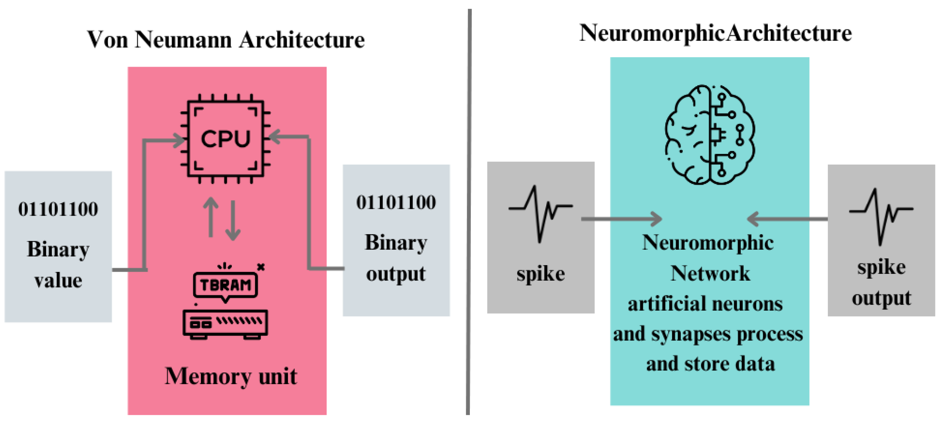
The human brain is a marvel of evolutionary engineering, a system of astonishing complexity and efficiency. Its ability to process vast amounts of information and withstand disruptions is largely due to the elaborate networks of neurons and synapses. The efforts of modern science to replicate this natural efficiency through the development of artificial neural systems is, in essence, an attempt to externalize and actualize the implicit potential of nature’s order. This challenge has long eluded traditional computational models. Artificial Neural Networks despite their sophistication, are energy-intensive and cumbersome, requiring vast amounts of memory and processing power to account for the temporal variability of events that unfold over varying durations and intensities. These systems, while useful, often fall short of capturing the full complexity of nature’s patterns. Enter Spiking Neural Networks, a new class of bio-inspired models that draw directly from the brain’s way of processing information. Unlike conventional neural networks, which operate continuously, SNNs rely on discrete spikes, closely mimicking the time-based behavior of biological neurons. This ability to handle time-varying information efficiently mirrors the brain’s rhythms and offers a more energy-conscious solution to understanding dynamic systems.

Keywords: 
;  ;  ;  ;  ;  ;  

1. Introduction

Early theories on the structure and functions of the brain were influenced by the Greek physician and philosopher Alcmaeon ([1]). He maintained that perception and intelligence originated in the brain and that the brain was essential to both sensory processing and cognitive processes. Later beliefs regarding the significance of the brain in comprehending human behavior and awareness derived from Alcmaeon’s thoughts, a departure from the prevailing view at the time which placed the heart at the center of cognitive functions. Plato postulated that the brain had a part in cognition; but, in Timaeus, thought and movement are functions of the rational (qua divine) aspect of the soul, which the Demiurge places in the head ([2]). The father of comparative anatomy, Aristotle (384–384), thought of the brain as a cooling organ that acted to balance the heat produced by the heart. In terms of its function in perception and cognition, he characterized the brain as a secondary organ that is dependent on the heart ([1,3,4]. Galen posited that it was the brain where the rational soul resided, with its principal functions of sensation and voluntary motion made possible by its first instrument (prôton organon), the psychic pneuma, elaborated in the ventricles. This pneuma, both as substance and as quality, was then transmitted through the alleged hollows of the nerves and thence by the insinuations of the ends of the nerves with the muscles to produce voluntary motion. The pneumatic function of sense perception remained relatively unexplored, beyond stating that pneuma as substance (ousia) in the optic nerve accounted for the change in the size of the pupil of the eye, while pneuma considered as a quality (poiotês) was responsible for the production of the visual image ([2]). In the Middle Ages, it was commonly believed that different mental faculties resided in specific areas within the brain’s ventricles. This theory, often attributed to ancient scholars and later linked with Galen, developed gradually over centuries before becoming fully formed in the Middle Ages ([5]). Al-Tabari (838-870 A.D.), in his medical encyclopedia "Firdous al-Hikmah" (Paradise of Wisdom), acknowledged the significance of the brain as the center of intellect and intelligence. He explained the functions of each of its many components, such as the ventricles, cranial nerves, and cerebral hemispheres. Al-Tabari also covered how the brain regulates bodily motions and feelings and how it plays a part in higher-order cognitive functions including memory, perception, and reasoning. He explained that the brain is made up of several chambers, or ventricles, that are filled with cerebrospinal fluid. The anterior (sometimes known as the first), middle (also known as the second), and posterior (also known as the third) ventricles are the three primary ventricles that Galen recognized. He thought that these ventricles greatly aided the management of mental functions and the processing of sensory information. Galen also put out the idea of ventricular localization, which postulated a connection between particular brain ventricles and distinct mental processes. He thought, for instance, that the front ventricle was linked to intellect, the middle ventricle to imagination, and the posterior ventricle to memory ([1,3,4,6]. In his medical writings, Mohammad bin Zakariya Rhazi (850-923 A.D), made important observations about the structure of the brain. He elucidated the structure and function of various brain regions, including the cerebral hemispheres, cerebellum, and brainstem. During the Islamic Golden Era, his discoveries about the structure of the brain and nerves advanced medical knowledge and had an impact on later advances in anatomy and neuroscience. In The Canon of Medicine, Ibn Sina detailed the trajectory of the optic nerves, noting their crossing at the optic chiasm for the integration of visual stimuli from both eyes into a single image. He suggested that the contralateral lateral ventricle processes this information, with the middle and posterior ventricles serving as processing chambers. Modern anatomy confirms the optic chiasm as the point of partial decussation of optic nerves, facilitating binocular vision and depth perception ([7]). Recent findings have reshaped our comprehension of the development, connectivity, and adaptability of the human cerebral cortex, a layer containing roughly 10 billion neurons organized into distinct areas specializing in processing various sensory, motor, and cognitive functions ([8]). The integration of the cortex during its early development incorporates inputs from the thalamus and brain stem axons, as well as midline patterning centers and basal ganglia primordia. The telencephalic vesicles give rise to a homogeneous ventricular zone from which the cortex, or pallium, further divides into ventral, lateral, dorsal, and medial pallium. Specific connections with other brain regions are established through the guidance of axons originating from cortical neurons. Axon guidance molecules, such as Ephrins, Semaphorins, and Netrins, provide cues that direct the growth of axons towards their target regions. Thalamocortical projections, for example, are guided by molecular signals expressed in the thalamus and cortex, ensuring precise connectivity between thalamic nuclei and their corresponding cortical areas. Once connections are established, cortical areas develop unique processing networks through the refinement of synaptic connections and the activity-dependent shaping of neuronal circuits. Neuronal activity, driven by sensory inputs and intrinsic circuitry, they are essential in shaping the functional properties of cortical neurons and their connectivity patterns. Hebbian plasticity mechanisms, such as long-term potentiation (LTP) and long-term depression (LTD), strengthen or weaken synaptic connections in response to correlated neuronal activity, contributing to the formation of specific processing networks.
While our understanding of the human brain has evolved throughout time, from the ancients who considered the brain as the seat of the soul and the sensorium commune linked to sensation and voluntary motion, with blood and liver/heart acting as soul carriers ([9,10]), Freud’s neurobiological model of the brain including concepts like ego, somatic drives, cathexes of psychic energy, wish fulfillment, and primary and secondary process ([11]), to the era of radio where memory processing and distributed cortical and limbic brain regions are associated with high-frequency oscillations, spanning a wide range of frequencies ([12]). Over time, our comprehension of the brain and the terminology we employ to elucidate its functions has strongly relied on the language and comprehension of contemporary technological endeavors. Thus, it should come as no surprise that modern-day human brain neurobiological definitions view the brain as an incredibly complex computing system made of "circuits", and "neuronal computation" and comprising approximately 100 billion neurons interconnected by "networks" of an estimated 100 trillion synapses ([13]). So how can we draw upon the brain’s mechanisms to improve the effectiveness of neural network design?

2. Neuromorphic Computing vs Biological Neuromorphic Systems

Nature provides numerous instances of compact, energy-efficient, flexible, and intelligent systems. Even in a basic creature like the bee, we observe remarkable flight capabilities and cognitive functions, despite its body weight being less than a gram and its brain consuming only around 10 milliwatts of power ([14]). Neuromorphic computing stems from the ambition to develop brain-like technology and aims to replicate the remarkable computational abilities of the human brain. With the advent of neural networks, modern computers have achieved remarkable feats in various cognitive tasks. However, the computational cost of such activities remains a concern. The human brain, operating on a power budget of around 20W ([15]), excels in tasks like simultaneous recognition, reasoning, and control, outperforming standard computers in terms of efficiency. Neuromorphic computing endeavors to foster the brain’s principles by emulating its structure and functionality. It harnesses the principles of neuroscience, particularly the vast connectivity of neurons and the time-dependent nature of neural activity ([15]). Unlike conventional computers, neuromorphic systems co-locate computation and memory, mimicking the brain’s architecture. These systems employ spike-based event-driven computations, which are more energy-efficient compared to traditional digital circuits. Neuromorphic computing comprises both hardware and algorithmic aspects, intending to enable energy-efficient artificial intelligence. It explores various learning mechanisms and hardware implementations, including analog and digital neuromorphic systems. The field emphasizes a symbiotic approach between hardware and software to achieve optimal energy efficiency and accuracy in spike-based computing. Deep learning employs artificial neural networks, which are commonly implemented on computers following the traditional von Neumann architecture, predominantly processing information sequentially. Figure 1 depicts the difference between the Neuromorphic architecture and the Von Neumann architecture.
Conversely, the brain’s hardware functions in a highly parallel manner, characterized by dense interconnections among neurons ([17]). Neurons also adhere to the Hebbian learning rule: neurons that fire together, wire together ([18]). This adaptability is believed to underlie learning and memory processes and plays a significant role in information processing within the brain. As a result of this structure, the brain exhibits remarkable energy efficiency, especially in tasks related to pattern recognition and classification, in contrast to conventional computers. To accomplish real-time and energy-efficient execution of Spiking Neural Network simulations, employing (digital, analog, or mixed-signal) hardware for implementation is essential instead of relying on (CPU or GPU-based) software simulations. Using hardware for SNN implementation in machine learning tasks holds promise for significantly reducing power consumption compared to conventional Artificial Neural Network approaches ([19]). Essentially, there are three neuromorphic components:
  • Neuromorphic sensors: By imitating the structure and function of neurons in electronic devices, neuromorphic engineering opens up a new avenue for research into brain design. The goal of this effort is to use the brain’s effective computing architecture for next-generation artificial systems. This method is exemplified by neuromorphic microchips, which mimic biological sensing and spike-based neural processing to enable nervous system-like event-driven computing. Mostly silicon-based, these devices use transistors to simulate brain circuits because of similar physics, which makes computational primitives easier to implement. The address-event representation (AER), which transmits spikes together with address and timing information off-chip to enable flexible connection and low-latency event-driven computing, is essential to their operation ([14]). Event-based neuromorphic vision sensors offer low energy consumption, low latency, high dynamic range, and high temporal resolution, revolutionizing visual sensing in autonomous vehicles ([20]).
  • Neuromorphic software: The current AI algorithms diverge significantly from the complexities of biological neurons and synapses. Biological neurons exhibit traits beyond simple non-linear functions; they spike, possess leakiness, memory, stochasticity, and the ability to oscillate and synchronize. Moreover, they are spatially extended, with distinct functional compartments integrating signals from various areas. Similarly, biological synapses are more than analog weights; they function as leaky memories with diverse time scales and state parameters governing their modifications. Some synapses are highly stochastic, transmitting only a fraction of received spikes. Often overlooked components of the brain, such as dendrites and astrocytes, and are also necessary in neural computation and regulation. Integrating these nuanced properties into artificial neural networks is what constitutes neuroporphic software ([21]).
  • Neuromorphic hardware:The rise of deep networks and recent corporate interest in brain-inspired computing has sparked widespread curiosity in neuromorphic hardware, which aims to mimic the brain’s biological processes using electronic components. The potential of neuromorphic hardware lies in its ability to implement computational principles with low energy consumption, employing the intrinsic properties of materials and physical effects. Initially pioneered by Carver Mead, this field focused on exploiting transistor leakage current’s exponential dependence on voltage. In recent years, researchers have utilized a variety of physical phenomena to mimic synaptic and neuronal properties. Neuromorphic hardware systems offer novel opportunities for neuroscience modeling, benefiting from parallelism for scalable and high-speed neural computation. However, despite the emerging memory technologies, such as flash memory and solid-state memory, that are enabling neuromorphic computing and bio-inspired learning algorithms like back-propagation, there’s a gap between the communities of software simulator users and neuromorphic engineering in neuroscience. ([22,23]).

3. Applications of SNNs

The bio-inspired approach of SNNs offers several advantages and has found applications in several fields. SNNs are particularly suited for tasks where asynchronous event-based data processing is involved, such as real-time event recognition, and sensory data analysis. and tasks that require efficient handling of spatiotemporal patterns. Moreover, SNNs are very good for low-power neuromorphic hardware implementations. They are also very appealing for applications in edge computing and Internet of Things (IoT) devices where energy efficiency is important. SNNs have shown promise in cognitive computing, robotics, pattern recognition, and brain-computer interfaces, which very boldly highlights their potential for advancing the field of artificial intelligence and neuroscience research:
  • Event-based Vision Sensors
    In recent years, researchers have combined event-based sensors with spiking neural networks (SNNs) to develop a new generation of bio-inspired artificial vision systems. These systems demonstrate real-time processing of spatio-temporal data and boast high energy efficiency. [24] utilized a hybrid event-based camera along with a multi-layer spiking neural network trained using a spike-timing-dependent plasticity learning rule. Their findings indicate that neurons autonomously learn from repeated and correlated spatio-temporal patterns, developing selectivity towards motion features like direction and speed in an unsupervised manner. This motion selectivity can then be harnessed for predicting ball trajectories by using a simple read-out layer consisting of polynomial regressions and trained under supervision. Thus, their study illustrates the capability of an SNN, coupled with inputs from an event-based sensor, to extract pertinent spatio-temporal patterns for processing and predicting ball trajectories.
    [25] propose a fully event-based image processing pipeline integrating neuromorphic vision sensors and spiking neural networks (SNNs) to enable efficient vision processing with high throughput, low latency, and wide dynamic range. Their approach focuses on developing an end-to-end SNN unsupervised learning inference framework to achieve near-real-time processing performance. By employing fully event-driven operations, they significantly enhance learning and inference speed, resulting in over a 100-fold increase in inference throughput on CPU and near-real-time inference on GPU for neuromorphic vision sensors. The event-driven processing method supports unsupervised spike-timing-dependent plasticity learning of convolutional SNNs, enabling higher accuracy compared to supervised training approaches when labels are limited. Furthermore, their method enhances robustness for low-precision SNNs by reducing spiking activity distortion, leading to higher learning accuracy compared to regular discrete-time simulated low-precision networks.
    [26] introduce Dynamic Vision Sensors (Event Cameras) for gait recognition, offering advantages like low resource consumption and high temporal resolution. To address challenges posed by their asynchronous event data, a new approach called Event-based Gait Recognition (EV-Gait) is proposed. This method utilizes motion consistency to remove noise and employs a deep neural network for gait recognition from event streams.
    [27] introduce the neuromorphic vision sensor as a novel bio-inspired imaging paradigm capable of reporting asynchronous per-pixel brightness changes known as ’events’ with high temporal resolution and dynamic range. While existing event-based image reconstruction methods rely on artificial neural networks or hand-crafted spatiotemporal smoothing techniques, this paper pioneers the implementation of image reconstruction via a deep spiking neural network architecture. Leveraging the computational efficiency of SNNs, which operate with asynchronous binary spikes distributed over time, the authors propose a novel Event-based Video reconstruction framework based on a fully Spiking Neural Network (EVSNN), using Leaky-Integrate-and-Fire (LIF) and Membrane Potential (MP) neurons. They observe that spiking neurons have the potential to retain useful temporal information (memory) for completing time-dependent tasks.
  • Bioinformatics
    Spiking neural networks (SNNs) are beginning to impact biological research and biomedical applications due to their ability to integrate vast datasets, learn arbitrarily complex relationships, and incorporate existing knowledge. Already, SNN models can predict, with varying degrees of success, how genetic variation alters cellular processes involved in pathogenesis, which small molecules will modulate the activity of therapeutically relevant proteins, and whether radiographic images are indicative of disease. However, the flexibility of SNNs creates new challenges in guaranteeing the performance of deployed systems and in establishing trust with stakeholders, clinicians, and regulators, who require a rationale for decision making. We argue that these challenges will be overcome using the same flexibility that created them; for example, by training SNN models so that they can output a rationale for their predictions. Significant research in this direction will be needed to realize the full potential of SNNs in biomedicine [28].
    Because interactions are important in biological processes, such as protein interactions or chemical bonds, this data is often represented as biological networks. The proliferation of such data has spurred the development of new computational tools for network analysis. [29] explore various domains in bioinformatics where NNs are commonly applied, including protein function prediction, protein-protein interaction prediction, and in silico drug discovery. They highlight emerging application areas such as gene regulatory networks and disease diagnosis, where deep learning serves as a promising tool for tasks like gene interaction prediction and automatic disease diagnosis from data. By extension, SNNs could be a great alternative to deep learning in these domains.
    As biotechnology advances and high-throughput sequencing becomes prevalent, researchers now possess the capability to generate and analyze extensive volumes of genomic data. Given the large scale of genomics data, many bioinformatics algorithms rely on machine learning techniques, with recent emphasis on deep learning, to uncover patterns, forecast outcomes, and characterize disease progression or treatment [30]. The progress in deep learning has sparked significant momentum in biomedical informatics, leading to the emergence of novel research avenues in bioinformatics and computational biology. Deep learning models offer superior accuracy in specific genomics tasks compared to conventional methodologies, using SNNs in these domain could prove to be a great alternative.
  • Neuromorphic Robotics
    Initially, robots were developed with the primary objective of simplifying human life, particularly by undertaking repetitive or hazardous tasks. While they effectively fulfilled these functions, the latest generation of robots aims to surpass these capabilities by engaging in more complex tasks traditionally executed by intelligent animals or humans. Achieving this goal necessitates drawing inspiration from biological paradigms. For instance, insects demonstrate remarkable proficiency in solving complex navigation challenges within their environment, prompting many researchers to emulate their behavior. The burgeoning interest in neuromorphic engineering has motivated the presentation of a real-time, neuromorphic, spike-based Central Pattern Generator (CPG) applicable in neurorobotics, using an arthropod-like robot as a model. A Spiking Neural Network was meticulously designed and implemented on SpiNNaker to emulate a sophisticated, adaptable CPG capable of generating three distinct gaits for hexapod robot locomotion. Reconfigurable hardware facilitated the management of both the robot’s motors and the real-time communication interface with the SNN. Real-time measurements validate the simulation outcomes, while locomotion trials demonstrate that the NeuroPod can execute these gaits seamlessly, without compromising balance or introducing delays. ([?])
  • Brain-Computer Interfaces
    [31] claim that Brain-Inspired Spiking Neural Network (BI-SNN) architectures offer the potential to extract complex functional and structural patterns over extensive spatio-temporal domains from data. Such patterns, often represented as deep spatio-temporal rules, present a promising avenue for the development of Brain-Inspired Brain-Computer Interfaces (BI-BCI). The paper introduces a theoretical framework validated experimentally, demonstrating the capability of SNNs in extracting and representing deep knowledge. In a case study focusing on the neural network organization during a Grasp and Lift task, the BI-BCI successfully delineated neural trajectories of visual information processing streams and their connectivity to the motor cortex. Deep spatiotemporal rules were then utilized for event prediction within the BI-BCI system. This computational framework holds significance in uncovering the brain’s topological intricacies, offering potential advancements in Brain-Computer Interface technology.
  • Space Domain Awareness
    With space debris posing significant threats to space-based assets, there is an urgent need for efficient and high-resolution monitoring and prediction methods. This study presents the outcomes of the NEU4SST project, which explores Neuromorphic Engineering, specifically leveraging event-based visual sensing combined with Spiking Neural Networks (SNNs), as a solution for enhancing Space Domain Awareness (SDA). The research focuses on event-based visual sensors and SNNs, which offer advantages such as low power consumption and precise high-resolution data capture and processing. These technologies enhance the capability to detect and track objects in space, addressing critical challenges in the Space domain. [32] propose an approach with potential to enhance SDA and contribute to safer and more efficient space operations. Continued research and development in this field are essential for unlocking the full potential of Neuromorphic engineering for future space missions.
So what ideas can we glean from studying the brain to enhance the efficiency of neural network construction? Is it feasible to replicate the complex genetic composition of neurons, even at the molecular level? And how can we mimic a system that remains largely incomprehensible to us?

4. Fundamentals of Spiking Neural Networks

[33] introduced SNNs as the third generation of neural network models. According to the analysis, neural network models could be categorized into three generations based on their computational units:
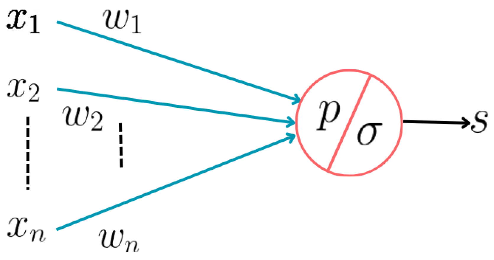
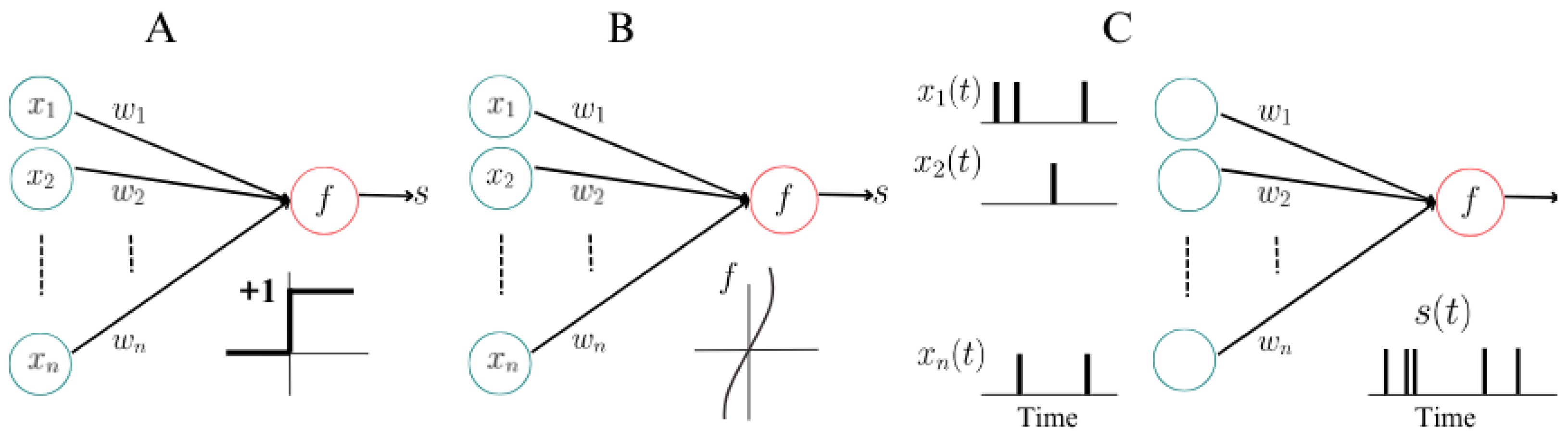
  • First Generation: Starting from their examination of key neuronal characteristics, McCulloch and Pitts aimed to represent the functional framework rather than the physical structure of neurons, essential for their functioning. They delineated five key functions: stimulus reception ( x 1 , x 2 , . . . , x n ) , stimulus weighting (synaptic coefficients w 1 , w 2 , . . . , w n ) , computation of the weighted stimulus sum ( p ) , establishment of a stimulation threshold σ for transmission initiation, and stimulus output ( s ) , as seen in Figure 2. Their model emphasizes the sequential arrangement of these functions, focusing only on their conceptual representation rather than the integration of factors fulfilling these functions. It’s important to note that this model represents abstract functions rather than observable phenomena, lacking any depiction of the neuronal cell’s internal material structure, which contributes to explaining the neuronal response to stimuli ([34]). Examples include multilayer perceptrons, Hopfield nets, and Boltzmann machines. They are universal for computations with digital input and output and can compute boolean functions.
  • Second Generation: Computational units apply activation functions with a continuous set of possible output values to a weighted sum of inputs. This generation includes feedforward and recurrent sigmoidal neural nets, as well as networks of radial basis function units. They can compute boolean functions with fewer gates than first-generation models and handle analog input and output.
  • Third Generation: This generation employs spiking neurons, or integrate-and-fire neurons, as computational units, inspired by experimental evidence indicating that many biological neural systems use the timing of single action potentials to encode information. These models reflect acumen from neurobiology research and aim to capture the timing of neural spikes for information processing.
Figure 3 illustrates the evolution of neural networks across generations. SNNs were inspired by the brain’s communication architecture, which uses discrete action potentials (spikes) in time through adaptive synapses to convert information [36]. Research on cortical pyramidal neurons has revealed that the timing of individual spikes plays an important part in encoding information within numerous biological neural networks ([37]).

4.1. Spiking Neurons

With approximately 10 11 spiking neurons, the human brain boasts a comparable scale to modern supercomputers, which also house a vast number of transistors. However, unlike supercomputers that consume megawatts of power (e.g., the K computer’s energy usage equates to that of 10,000 suburban homes), the brain operates on a mere 30 W. This stark contrast makes the brain an alluring model for energy-efficient computing. To harness this potential, it’s imperative to decipher the organization of spike-based computations within the brain ([38]).
In Wolfgang Maass’s seminal paper titled "Lower Bounds for the Computational Power of Networks of Spiking Neurons," an in-depth analysis is conducted to discern the computational capabilities of Spiking Neural Networks (SNNs) in comparison to Turing machines, the latter being foundational in theoretical computer science. SNNs, inspired by the complex workings of the human brain, operate through the transmission of discrete spikes or pulses between neurons, thereby encoding and processing information. Maass’s exploration focuses on unraveling the potential computational power embedded within these networks, delving into their ability to execute complex computations.
In another work, [39] explore the computational power of Networks of Spiking Neurons (SNNs). According to the findings, a deterministic network of spiking neurons theoretically possesses the same computational capability as a universal Turing machine. This suggests that such networks can utilize the lengths of interspike intervals to encode and transmit information efficiently. However, observations from biological data challenge this deterministic perspective. Observations indicate that brain computations are non-deterministic in nature. When attempting to induce the brain to perform the same computation repeatedly, significant variations in spiking activity occur from trial to trial. This variability in spiking patterns reflect the probabilistic nature of neural computation within the brain, which diverges from the deterministic framework assumed by traditional computing models.

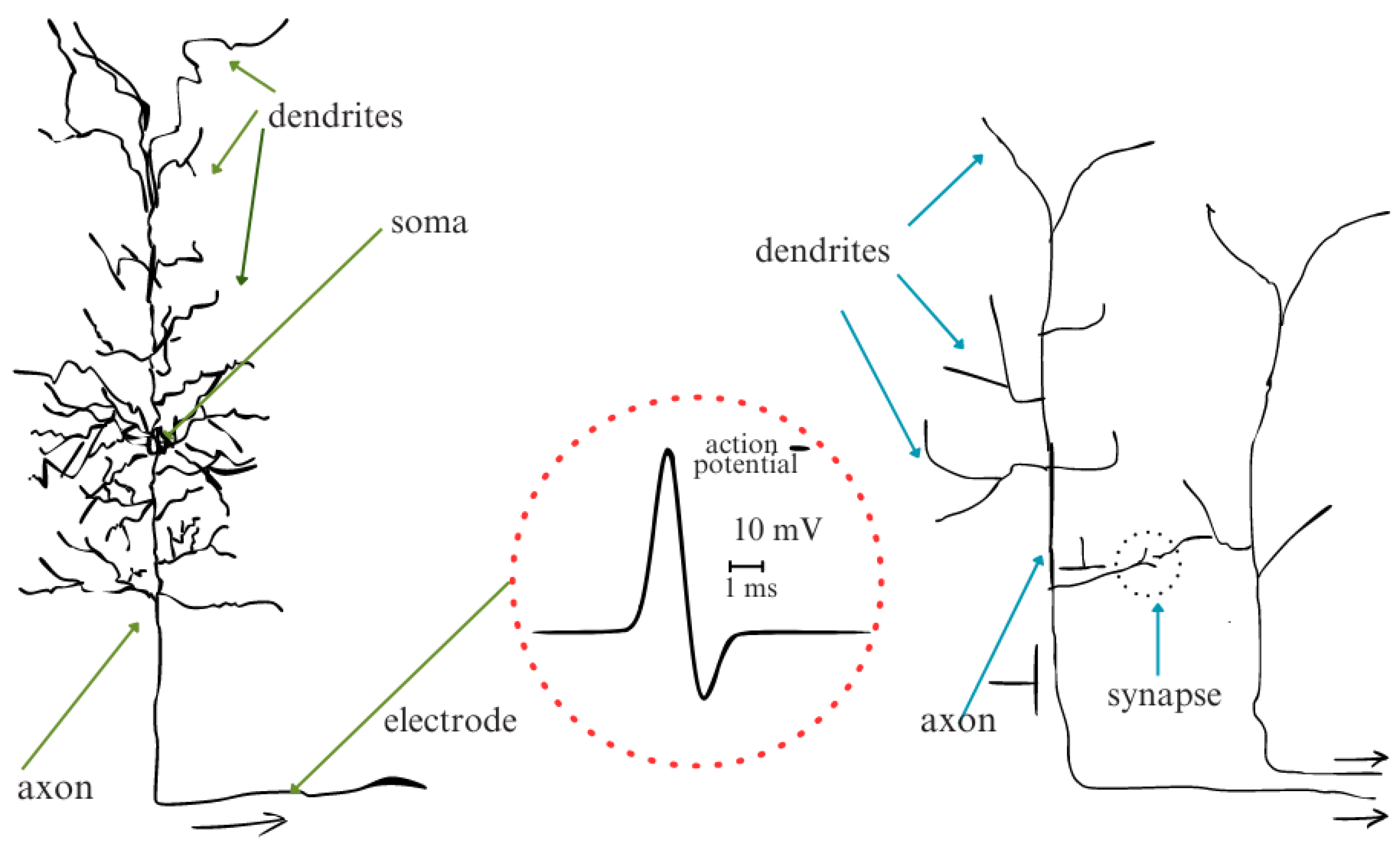
4.2. Biological Neuron Model

Over the last century, extensive biological studies have amassed a wealth of relevant information regarding the composition and operations of the brain. Neurons, the fundamental units responsible for processing information within the central nervous system, form complex interconnections with one another. A fragment of such neural network structure is depicted in Figure , illustrating a sketch by Ramón y Cajal, a prominent figure in neuroscience during the early 1900s. Within this depiction, one can discern several neurons characterized by triangular or circular cell bodies, each adorned with elongated, wire-like extensions.
Figure 4. A sketch by Ramón y Cajal depicts several neurons observed within the mammalian cortex under the microscope. It’s important to note that only a fraction of the neurons present in the cortical tissue sample are visible due to the staining process; the actual density of neurons is significantly higher. Dendrites emanate from the cell laterally and upwards, distinguishable by their textured surface. Meanwhile, the axons are identifiable as slender, unblemished lines that extend downwards with occasional branching to the left and right ([40,41]).
Preprints 145617 g004
Figure 5. Presented here are multiple layers of pyramidal cells situated in the superior temporal gyrus, which shares a similar layered structure with other regions of the temporal cortex. While they exhibit variations in size and positioning, all pyramidal cells (labeled a, b, c, d, e, f, g, h) showcase the characteristic cone-shaped cell body, a solitary apical dendrite projecting upwards towards the cortical surface, as well as basal dendrites and axons (labeled a). Cajal extensively characterized pyramidal cells across various tissues, elucidating the diverse shapes and sizes encountered throughout the brain. Additionally, he proposed that the dendritic arborizations of pyramidal cells would undergo size and shape variations throughout an organism’s lifespan. Recent studies indicate that the pyramidal cells depicted here, extracted from the superior temporal gyrus of an infant, possess considerably larger and denser dendritic branches compared to those typically found in adults within the same location ([40,41]).
Preprints 145617 g005

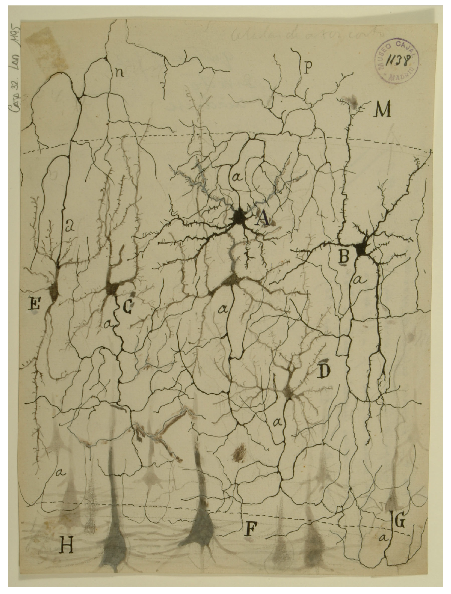
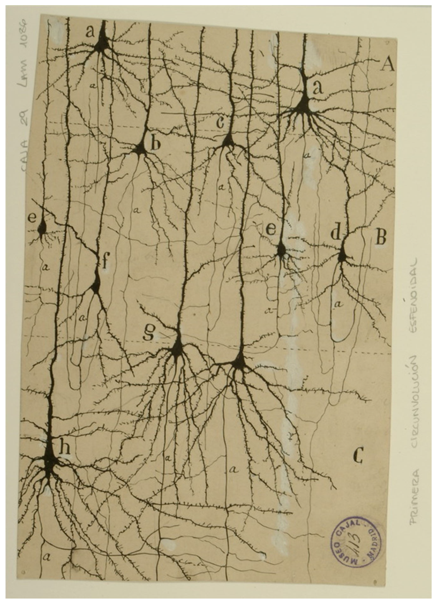
4.2.1. Neuronal Elements

A spiking neuron is a type of neuron that generates action potentials or depolarization of the cell membrane voltage. The neuron can fire repeatedly in response to stimuli. Action potentials arise from the opening and closure of voltage-gated ion channels. Spike frequency adaptation occurs when the degree of opening can be regulated by the membrane voltage. Spike frequency coding allows rapid, high-speed communication of information. It is a type of neuron activated by an input signal and generates a series of short-lived action potentials in response, rather than a continuous electrical signal. The spike generation process is controlled by two types of ion channels: sodium channels, which are responsible for creating the up-spike, and potassium channels, which are responsible for creating the down-spike. The up-spike is produced when sodium channels are opened, allowing sodium particles to flow in, and resulting in a higher membrane voltage. The down-spike is produced when potassium channels are closed, causing the membrane voltage to drop.
A neuron, is made up of three parts: dendrites, soma, and axons. Dendrites receive electrical activity from other neurons; the soma acts as the central processing unit for the neuron, and the axon carries the electrical signal to other neurons, see Figure 6. When the neuron receives enough electrical activity, it fires an electrical signal down its axon, known as an action potential ([42]).
A neuron comprises a cell body, known as the soma, which contains numerous dendrites branching out to receive information from neighboring neurons. The neuron’s output, or axon, communicates information to other neurons through action potential pulses, commonly referred to as spikes. These spikes travel between neurons via synaptic connections, with each connection having a specific weight. The neuron maintains a membrane potential, influenced by factors such as the rate of incoming spikes, the spatial arrangement of neurons in the network, and the synaptic weights. When the combined weight of input spikes surpasses a predetermined firing threshold, the neuron generates an output spike. This firing mechanism is integral to neural information processing ([43]). A neuron can send a signal across the space between itself and another neuron, which is called a synapse. The sending neuron is known as the pre-synaptic cell, and the receiving neuron is the target cell. The signals transmitted by neurons can take the form of short electrical pulses, which are known as action potentials or spikes. A typical action potential has an amplitude of around 100 millivolts and a duration of 1-2 milliseconds. The amplitude of an action potential is measured in millivolts. It is the difference in voltage between the resting potential, which is the voltage of the neuron when it is not receiving any input, and the voltage during an action potential. The voltage of the neuron is measured at the peak of the action potential and is usually recorded by placing an electrode near the soma or dendrite of the neuron. An action potential can have either a biphasic or triphasic shape, depending on its morphology ([44]). The shape of the action potential is the same within a single neuron, but the number and timing of spikes can carry important information. A spike train is a sequence of stereotyped action potential events that occur at regular or irregular intervals. Between spikes, there is an absolute refractory period, during which it is impossible to generate another spike ([45]).

4.2.2. The Synapse

The meeting point between the axon of one neuron and the dendrite (and/or soma) of another neuron is a biochemical connection known as a synapse. The space between the two cells forms a narrow gap known as the synaptic cleft. When an action potential reaches a synapse, it triggers a complex cascade of biochemical processes that lead to the release of neurotransmitter molecules from the presynaptic nerve cell. These molecules cross the synaptic cleft and are detected by specialized receptors on the surface of the receiving neuron. This initiation of a chemical signal results in changes in the cell membrane potential of the receiving neuron ([46]). The synapse is the normal anatomical relation between contiguous neurons, forming a junction between nerve cells and forming a connection between nerve cells and their glial cells ([47]).

4.2.3. Networks of Neurons

The neurons of the brain are embedded in a network of billions of other neurons and glial cells. The brain is organized into different regions and areas. The cortex, a thin sheet of neurons, can be thought of as a folded cover over other brain structures. Some cortical areas process sensory input, while others are involved in working memory or motor control. There are two main types of neurons in sensory cortices: simple cells and complex cells. Simple cells respond to limited regions of the visual field called the neuron’s receptive field. The receptive field of simple cells is elongated and heterogeneous ([48]).

4.2.4. Postsynaptic Potentials

When an action potential is received at a synapse, changes occur in the voltage across the membrane of the receiving neuron. This change is known as the membrane potential. The membrane potential is a value that is used to measure the polarization of the neuron. The resting membrane potential of the neuron is already strongly negative, at about -65 mV. An input from an excitatory synapse results in a decrease in the negative polarization of the membrane, which is considered to be a depolarizing event. Conversely, an input from an inhibitory synapse leads to an increase in the negative polarization of the membrane, known as a hyperpolarizing event.
Let’s consider the time u i ( t ) of the membrane potential of neuron i. Before the input spike has hit, we have u i ( t ) = u r e s t . At t = 0 the presynaptic neuron j fires its spike. For t > 0 , we see at the electrode a response of neuron i :
u i ( t ) u r e s t = : ϵ i j ( t )
Equation 1 defines the PSP, or the electrical potential in the receiving neuron. If the voltage difference, u i ( t ) u r e s t , is positive (negative), we have an EPSP (IPSP), or an excitatory (inhibitory) postsynaptic potential.
Consider two presynaptic neurons j = 1 , 2 , which both send spikes to the postsynaptic neuron i Neuron j = 1 fires spikes at t 1 ( 1 ) , t 1 ( 2 ) , . . . , , similarly neuron j = 2 fires at t 2 ( 1 ) , t 2 ( 2 ) , . . . , . Each spike evokes a postsynaptic potential ϵ i 1 or ϵ i 2 , respectively. As long as there are only few input spikes, the total change of the potential is approximately the sum of the individual PSPs:
u i ( t ) = j f ϵ i j ( t t j ( f ) ) + u r e s t
The spike afterpotential is a form of negative polarization. The duration and magnitude of the spike afterpotential can vary greatly, depending on the cell type and the intensity of the stimulus. The spike afterpotential can also contribute to the integration of signals at a particular synapse. For example, if the afterpotential is sufficient to drive the receiving neuron past its threshold, then the stimulus at the synapse will be integrated over time, leading to a cumulative effect. Conversely, the principle of linearity becomes disrupted when an excessive number of input spikes occur within a brief period. Once the membrane potential surpasses a critical threshold value ϑ , its trajectory diverges significantly from a mere summation of postsynaptic potentials (PSPs). At this juncture, the membrane potential undergoes a rapid and pulse-like excursion, with an approximate amplitude of 100 mV. This transient voltage pulse propagates along neuron i’s axon to synapses with other neurons. After the pulse, the membrane potential typically does not immediately revert to its resting state; instead, it often traverses a phase of hyperpolarization, falling below the resting potential. This hyperpolarization phase is termed the ’spike-afterpotential. Individual excitatory postsynaptic potentials (EPSPs) typically exhibit amplitudes within the range of one millivolt. The threshold value for initiating a spike is approximately 20 to 30 mV higher than the resting potential. For most neurons, the occurrence of four spikes, is insufficient to elicit an action potential. Instead, approximately 20-50 presynaptic spikes must occur within a brief temporal window to trigger a postsynaptic action potential ([40]).

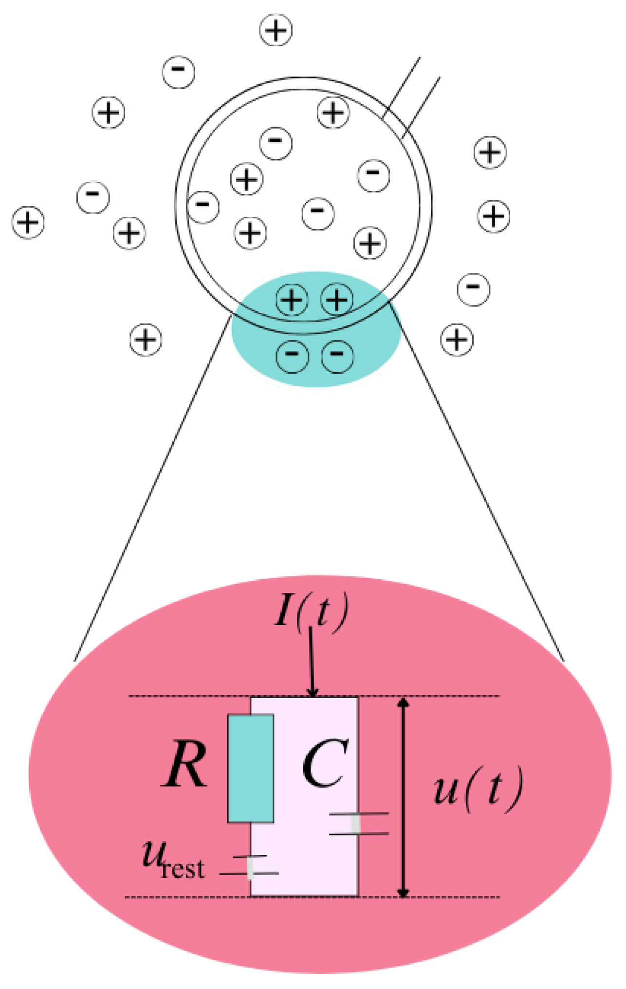
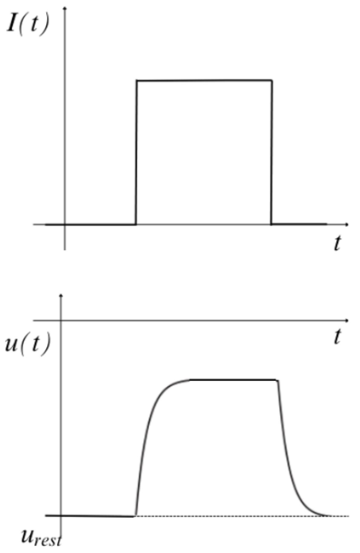
4.2.5. Integrate and Fire Model

For a rough approximation of neural dynamics, we consider the process as a combination of summation (or integration), as seen in Equation 2, and a mechanism that triggers action potentials. The firing times are defined as points in time when the membrane potential reaches a formal threshold ϑ . If the voltage u i ( t ) containing the summed effect of all inputs reaches ϑ from below, we say that neuron i fires a spike. The moment of this spike is the firing time t i ( f ) ([40,49]). An integrate-and-fire model is a type of neuron model that uses a simple and intuitive way to model the electrical activity of a neuron. The model captures the basic properties of a neuron, such as its ability to integrate input signals and generate output signals. The main idea behind an integrate-and-fire model is that the neuron’s electrical activity is determined by its "integrate" and "fire" states. When a neuron is in its integrate state, it receives and integrates input signals, which are represented as currents. When the total input reaching the neuron exceeds a threshold, it switches to the fire state, during which it releases an output signal, called an action potential. The neuron remains in the fire state for a brief period, after which it switches back to the integrate state. The duration of the fire state is determined by a parameter called the refractory period. After the refractory period has passed, the neuron can switch back to the integrate state ([50]). The integrate-and-fire model is a simplification of the neurological behaviour of the neuron. It is based on the theory that an action potential is a binary event, that is it only has two states: a "fired" state and a "not-fired" state. The model is based on two key features:
  • a differential equation that describes the evolution of the membrane potential
  • a threshold that defines the point where the membrane potential becomes a "fired" state ϑ
This simple model is referred to as the "leaky integrate-and-fire" model [50].

4.2.6. Electrical Theory Principles

The variable u i denotes the current state of neuron i’s membrane potential. When no external input is present, the potential remains at its resting state, u r e s t . Introducing a current I ( t ) or a synaptic input from other neurons alters the potential u i from its resting level. To establish an equation linking the current voltage u i ( t ) u r e s t to the input current I ( t ) , we use fundamental principles from electrical theory. Neurons are encompassed by a cell membrane, which serves as a relatively effective insulator. Injecting a brief current pulse I ( t ) into the neuron results in additional electrical charge q = I ( t ) d t , which must dissipate. This charge charges the cell membrane, behaving akin to a capacitor with capacity C. However, due to imperfections in the insulator, the charge gradually seeps through the membrane over time, characterized by a finite leak resistance R.
The fundamental electrical circuit of a leaky integrate-and-fire model comprises a capacitor C parallel with a resistor R driven by a current I ( t ) , see Figure ??and ??. In the absence of driving current I ( t ) , the voltage across the capacitor equals the battery voltage u r e s t . To examine the circuit, we apply the principle of current conservation and divide the driving current into two segments:
I ( t ) = I R + I C
The initial segment, I R , denotes the resistive current that traverses the linear resistor R. It can be determined using Ohm’s law as I R = u R / R , where u R = u u r e s t represents the voltage across the resistor. The subsequent segment, I C , serves to charge the capacitor C. Using the definition of capacity as C = q / u (where q denotes charge and u represents voltage), we ascertain the capacitive current I C = d q / d t = C d u / d t , hence:
I ( t ) = u ( t ) u r e s t R + C d u d t
We proceed by multiplying Equation 4 by R and introduce the time constant τ m = R C , representing the ’leaky integrator’. This manipulation results in the conventional form:
τ m d u d t = [ u ( t ) u r e s t ] + R I ( t )
Here, u denotes the membrane potential, and τ m signifies the membrane time constant of the neuron.
Mathematically, Equation 5 is viewed as a linear differential equation. In electrical engineering, it represents the equation of a leaky integrator or R C circuit, where resistor R and capacitor C are configured in parallel. Neuroscientists regard Equation 5 as the equation of a passive membrane.
To find the solution to Equation 5, let’s assume, for any given reason, that at time t = 0 , the membrane potential assumes a value of u r e s t + Δ u , with the input I ( t ) vanishing for t > 0 . Intuitively, we anticipate that, given ample time, the membrane potential will gradually return to its resting value u r e s t . Thus, the solution to the differential equation with the initial condition u ( t 0 ) = u r e s t + Δ u is as follows:
u ( t ) u r e s t = Δ u exp ( t t 0 τ m ) f o r t > t 0
Therefore, when there is no input, the membrane potential exponentially decreases towards its resting state. The membrane time constant τ m = R C indicates the characteristic time required for this decay process. In the case of a typical neuron, this time constant falls within the range of 10 milliseconds, which is notably longer compared to the duration of a spike, typically around 1 millisecond ([40]).
Figure 7. Electrical characteristics of neurons: the passive membrane. A neuron, surrounded by the cell membrane, depicted as a large circle, experiences a (positive) input current I ( t ) that elevates the electrical charge within the cell. The cell membrane functions akin to a capacitor alongside a resistor, connected in series with a battery having a potential of u r e s t , as shown in the zoomed inset ([40]).
Preprints 145617 g007
Figure 8. Electrical characteristics of neurons: the passive membrane. In response to a step current (depicted at the top), the cell membrane exhibits a gradual voltage response (illustrated at the bottom). Upon reaching a stable condition, the charge on the capacitor remains constant. Consequently, all input current is directed through the resistor. As a result, the steady-state voltage across the resistor amounts to R I 0 , thus yielding a total membrane voltage of u r e s t + R I 0 . ([40])
Preprints 145617 g008

4.2.7. The Threshold for Spike Firing

The expression "firing time" pertains to the instance when a specific neuron generates an action potential, denoted as t ( f ) . In the leaky integrate-and-fire model, the firing time t ( f ) is determined based on a threshold criterion, see Figure 9.
t f : u ( t f ) = ϑ
In the integrate-and-fire model, the properties of the spike are not described explicitly. The firing time is simply noted, and immediately after t ( f ) the potential is reset to a new value u r which is less than the threshold value ϑ :
lim δ 0 ; δ > 0 u ( t f + δ ) = u r
For t > t ( f ) , the dynamics of the leaky integrate-and-fire model is described by the differential equation 5. This equation is similar to the equation for the dynamics of the membrane potential but includes a term that incorporates the leak current. When the leaky integration model is combined with a resetting rule for firing that sets the potential to a new value of u r , it becomes the leaky integrate-and-fire model (LIF) described previously. The reset is defined by the equation 8 which sets the potential back to u r .

4.2.8. Limitations of LIF Model

The LIF model is defined by the differential equation 5, i.e:
τ m d u d t = [ u ( t ) u r e s t ] + R I ( t )
and the reset condition 8, i.e:
lim δ 0 ; δ > 0 u ( t f + δ ) = u r
where t ( f ) is the firing time:
t ( f ) = { t | u ( t ) = ϑ }
Integrated-and-fire neurons have a long history and are a common tool in modeling neural activity. The original Lapicque model ([52]), viewed the neuron as an electric circuit consisting of a resistor and capacitor in parallel, representing the leakage and capacitance of the neuron’s membrane. This simple model allowed Lapicque to calculate the spiking rate of a neuron. subsequent studies have refined Lapicque’s work, including Hill ([53]), who developed the concept of critical stimulation intensity in neural activity. The strength of this approach lies in its focus on subthreshold membrane properties and exclusion of mechanisms responsible for action potentials ([54]).
  • Integration of inputs is linear and independent of the state of the receiving neurons.
  • No memory of previous spikes is retained after a spike generation. Let’s examine these limitations and how they will be resolved in the extended leaky integrate-and-fire model.
  • Being deterministic, LIF neurons fail to capture the stochastic behavior inherent in biological neurons, leading to an oversimplification of neural activity.
  • The input current is assumed to be linear, which means that the response (the integrate-and-fire potential) is determined only by the value of the stimulus and not by the history of previous stimuli ([40]).
  • The model does not capture the slow processes in the neuron that are responsible for input adaptation (changes in membrane conductances).
  • The membrane Potential is always reset to the same value after a spiking event, irrespective of the state of the neuron.
  • LIF neurons struggle to accurately reproduce detailed spiking dynamics, such as adaptation and bursting, limiting their applicability in certain contexts.
  • The spatial structure of the cell, including the nonlinear interactions between different branches of the cell, is not taken into account.
  • The neurons are not just isolated but embedded into a network and receive multiple inputs from other neurons across all their synapses. If a few inputs arrive on the same branch of the neuron within a few milliseconds (ms), the first input triggers a change in the membrane potential that could affect the response to the subsequent inputs. This kind of non-linear response can also lead to saturation or amplification of the response depending on the kind of currents that are involved.
  • The LIF neuron model describes the membrane potential of a neuron, but does not include the actual changes in membrane voltage and conductances driving the action potential ([54].

4.2.9. Other Models

To effectively simulate neurons in vivo, it’s imperative to consider the seemingly erratic arrival times of synaptic inputs. Early attempts to incorporate stochastic activity into the integrate-and-fire model introduced the concept of modeling incoming postsynaptic potentials (PSPs) as a random walk, as demonstrated by [55]. Subsequent advancements primarily relied on this diffusion approach, employing stochastic differential equations and the Ornstein–Uhlenbeck process as elaborated by [56].
Stein extended the integrate-and-fire model to contain stochastic input, aggregating the decay of membrane potential in works from 1965 and 1967. Following this, various researchers, including [57,58,59,60,61], further explored the model using stochastic differential equations and numerical methods. These techniques were instrumental in investigating aspects such as the role of inhibition, the effect of reversal potentials, and other features within the Stein model.
The Hodgkin–Huxley model, introduced by [62], describes the neuron membrane potential based on the dynamic behavior of ion channels in the soma and dendrites. With the advent of increased computational resources, it’s now feasible not only to numerically simulate Hodgkin–Huxley model neurons with multiple ion channels and spatial compartments but also to analyze the behavior of small networks of such neurons. However, these complex computational models face several challenges. They often lack intuitive acumen into neuronal dynamics, involve numerous parameters making exploration of parameter space challenging, and cannot be analytically analyzed.
These studies acknowledge that there are some limitations to this approach as well. First, like any phenomenological model, it is not possible to gain an accurate understanding of the underlying neural mechanisms and the parameters. Second, these models are often based on simplified assumptions and do not reflect the complexity of biological neurons. Despite these limitations, phenomenological models provide a computationally efficient and simplified way to study the overall behavior of neuronal circuits and can shed light on important neural mechanisms such as memory or learning. Further research on the appropriate trade-off between biological detail and computational efficiency is needed in order to develop better models for network studies ([37]).

4.2.10. Spike Encoding and Decoding

The human brain, the most sophisticated and energy-efficient computing system, processes information through the interaction and communication among neurons, transmitting information via action potentials (spikes). Sensory information is encoded in spike patterns, which constitute various neural coding schemes ([63,64,65]. These schemes, including rate coding, temporal coding, phase coding, and burst coding, represent the mechanisms of information transmission and processing. Rate coding ([66]), relying on spiking rates, has been dominant in neuroscience and ANNs due to its simplicity and robustness. However, it suffers from slow information transmission. Temporal coding uses precise spike timing to convey information rapidly ([67]), such as time to first spike (TTFS) coding, which enables super-fast transmission speeds ([68]). Phase coding correlates spike phases with background oscillation rhythms and has shown faster inference speeds compared to rate coding in SNNs ([69]). Burst coding, observed in various parts of the nervous system, involves bursts of spikes that are reliable in information transfer and can enhance energy efficiency and processing speed in SNNs ([70]).
In SNNs, input signals are encoded in the form of spike patterns: sequences of spikes that are generated at specific times. The output of the network is then decoded based on the pattern and timing of the spikes generated in response to the input. Different SNNs can encode and decode input and output signals in different ways, but generally the encoding (input) process involves encoding the input signals into spike patterns and the decoding (output) process involves decoding the spike patterns into outputs. The importance of input encoding and output decoding for the success of SNNs is well-recognized in the neural computing research community. Input encoding is an essential step in converting sensory data into a format suitable for processing by SNNs. Appropriate input encoding techniques play a key role in ensuring the performance of SNNs for various applications. On the other hand, output decoding aims to interpret the spiking activity of SNNs to extract meaningful information from the network, such as making decisions or classifying inputs. This process is an integral part of the end-to-end system that drives SNNs. Different encoding schemes can be used depending on the nature of the input data and the requirements of the task.
1) 
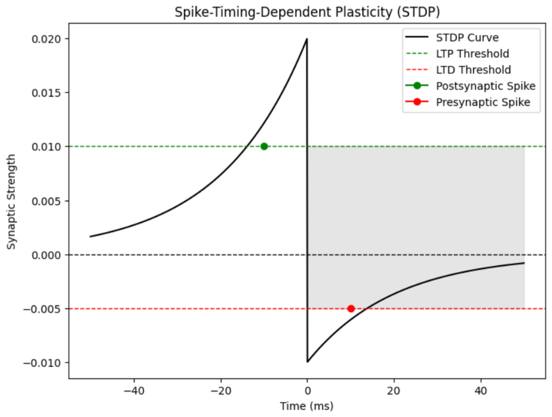
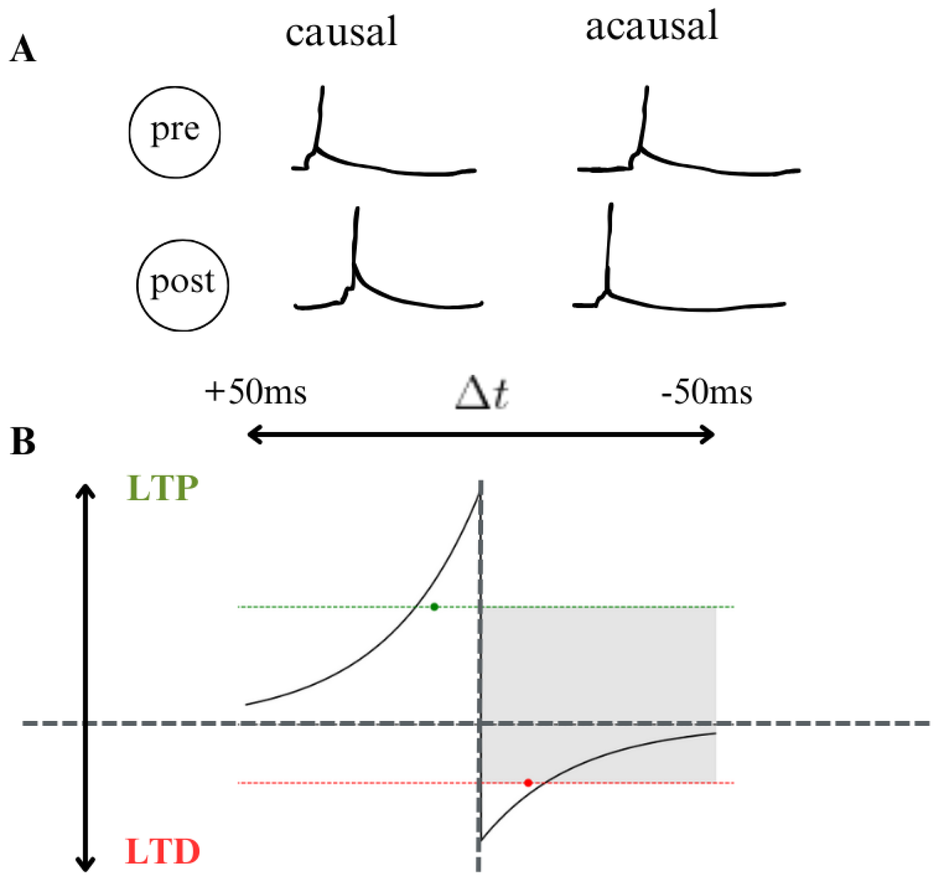
Spike Timing Dependent: Electrical activity plays an important role in shaping the structure and function of neural circuits over an organism’s lifespan ([71,72]). Changes in sensory experiences that disrupt normal patterns of activity can lead to significant remodeling of neural networks and alterations in neural response properties. Learning and memory processes are also thought to rely on activity-dependent modifications in neural circuits. Recent discoveries regarding spike timing-dependent plasticity (STDP) have garnered significant interest among researchers and theorists, particularly in understanding cell type-specific temporal windows for long-term potentiation (LTP) and long-term depression (LTD). Beyond the conventional correlation-based Hebbian plasticity, STDP offers new avenues for exploring information encoding, circuit plasticity, and synaptic learning mechanisms. Key questions arise regarding the dependence of activity-induced modifications at GABAergic synapses on the precise timing of pre and postsynaptic spiking, the presence of STDP in neuronal excitability and dendritic integration, and the impact of complex neuronal spiking patterns, including high-frequency bursts, on STDP. Additionally, researchers seek to elucidate how STDP influences the operation of neural circuits and higher brain functions, such as sensory perception. Understanding the cellular mechanisms underlying such functional plasticity has been a longstanding challenge in neuroscience ([73]). Hebb’s influential postulate on the cellular basis of learning proposed that repeated or persistent activation of one neuron by another leads to structural or metabolic changes that enhance the efficiency of synaptic transmission between them([74]). Experimental findings supporting this postulate came with the discovery of long-term potentiation (LTP), initially observed in the hippocampus and later identified in various neural circuits ([75]), including cortical areas, the amygdala, and the midbrain reward circuit ([76,77]). LTP is typically induced by high-frequency stimulation of presynaptic inputs or by pairing low-frequency stimulation with strong postsynaptic depolarization. Conversely, long-term depression (LTD) is induced by low-frequency stimulation, either alone or paired with mild postsynaptic depolarization ([78,79]). Together, LTP and LTD enable bidirectional modification of synaptic strength in an activity-dependent manner, making them plausible candidates for the synaptic basis of learning and memory. In other studies, the induction of LTP and LTD has been found to be influenced by specific types of neural activity ([80]). See Figure 10.
2) 
Phase Encoding: Phase encoding refers to a neural coding strategy where information is represented not only by the number of spikes (spike count) but also by the precise timing of spikes relative to the phase of ongoing network oscillations. In the study conducted on the primary visual cortex of anesthetized macaques, researchers found that neurons encoded rich naturalistic stimuli by aligning their spike times with the phase of low-frequency local field potentials (LFPs). The modulation of both spike counts and LFP phase by the presented color movie indicated that they reliably conveyed information about the stimulus. Particularly, movie segments associated with higher firing rates also exhibited increased reliability of LFP phase across trials. Comparing the information carried by spike counts to that carried by firing phase revealed that firing phase conveyed additional information beyond spike counts alone. This extra information was used for distinguishing between stimuli with similar spike rates but different magnitudes. Thus, phase encoding allows primary cortical neurons to represent multiple effective stimuli in an easily decodable format, enhancing the brain’s ability to process and interpret sensory information. [81] explored the concept of phase encoding in neural responses to visual stimuli by analyzing the relationship between spike times and the phase of ongoing local field potential (LFP) fluctuations. The research involved recording neural signals in the primary visual cortex of anesthetized macaques while presenting a color movie. The power of the LFP spectrum was found to be highest at low frequencies (<4 Hz) during movie presentation, indicating the modulation of LFP phase by the visual stimulus. To investigate the potential encoding of information beyond spike count, the study examined the phase at which spikes occurred relative to LFP fluctuations. By labeling spikes based on their phase quadrant, the researchers sought to predict visual features more effectively than through spike counts alone. Results suggested that phase coding could enhance stimulus discrimination, especially in scenarios where spike rates were comparable. Analysis of LFP-phase reliability and spike-phase relationships demonstrated the potential of phase-of-firing coding to convey additional information about visual stimuli. The study utilized Shannon information analysis to quantify the amount of information conveyed by spike times relative to LFP phase. Results indicated that phase-of-firing coding in the 1–4 Hz LFP band provided 54% more information about the movie compared to spike counts alone. This finding suggests that phase encoding may play a significant role in representing visual information in the primary visual cortex, offering a novel perspective beyond traditional spike-count coding. Increasing evidence suggests that ongoing oscillations’ phases are necessary in neural coding, yet their overall importance across the brain remains unclear. [82] investigated single-trial phase coding in eight distinct regions of the human brain —four in the temporal lobe and four in the frontal lobe—by analyzing local field potentials (LFPs) during a card-matching task. Our findings reveal that in the temporal lobe, classification of correct/incorrect matches based on LFP phase was notably superior to classification based on amplitude and nearly equivalent to using the entire LFP signal. Notably, in these temporal regions, the mean phases for correct and incorrect trials aligned before diverging to encode trial outcomes. Specifically, neural responses in the amygdala suggested a mechanism of phase resetting, while activity in the parahippocampal gyrus indicated evoked potentials.
3) 
Rate Encoding: is a prevalent coding scheme employed in neural network models. In this scheme, each input pixel is interpreted as a firing rate and is transformed into a Poisson spike train with the corresponding firing rate. The input pixels undergo scaling by a factor λ , typically set to four for optimal classification and computational efficiency. This scaling ensures that the firing rates are limited between 0 and 63.75 Hz. The generation of Poisson spike trains involves comparing the scaled pixels with random numbers to determine the occurrence of spikes.
4) 
Population Encoding: In any effective democracy, the influence of individual neurons is minimal; what truly matters is the collective activity of populations of neurons. For instance, in tasks like controlling eye and arm movements, or discerning visual stimuli in the primary visual cortex, the precision achieved far surpasses what could be expected from the responses of individual neurons. This is unsurprising, as single neurons provide limited information, necessitating some form of averaging across populations to obtain accurate sensory or motor information. However, the precise mechanisms underlying this averaging process in the brain, particularly how population codes are utilized in complex computations (like translating visual cues into motor actions), remain incompletely understood ([83]). This type of encoding is also referred to as frequency encoding.
A significant challenge in comprehending population coding arises from the inherent noise in neurons: even when presented with the same stimulus, neuronal activity exhibits variability, making population coding inherently probabilistic. Consequently, a single noisy population response cannot precisely determine the stimulus; instead, the brain must compute an estimate of the stimulus or a probability distribution over potential stimuli. The accuracy of stimulus representation and the impact of noise on computations depend heavily on the nature of neuronal noise, particularly whether the noise is correlated among neurons. The encoding perspective examines how correlations impact the amount of information in a population code. This question lacks a straightforward answer, as correlations can increase, decrease, or leave the information unchanged, depending on their structure. While this may seem disappointing, it emphasizes the importance of understanding correlation details. General statements about correlations always helping or hurting are ruled out. To assess the impact of correlations on the information content within a population code, it’s essential to evaluate the information contained in the correlated responses, represented as I, and juxtapose it against the information that would be present if the responses were uncorrelated, denoted as I s h u f f l e d . The term I s h u f f l e d originates from the practice of decorrelating responses in experiments by shuffling trials. The difference between these two measures, denoted as Δ I s h u f f l e d I I s h u f f l e d , serves as a metric for gauging the influence of correlations on the information content within a population code. This method is significant because it allows for the quantification of information, enabling computation from empirical data.. This approach relies on quantifiable information computed from data. Understanding the impact of correlations on information can be illustrated using a two-neuron, two-stimulus example. Despite its small size, this example retains key features of larger population codes. By plotting correlated and uncorrelated response distributions and analyzing their features, we gain better understanding of the relationship between signal, noise, and information in pairs of neurons. The figure illustrates correlated and uncorrelated response distributions using ellipses to represent 95% confidence intervals ([83]).
5) 
Burst coding: Burst coding is a neural information transmission strategy that involves sending a burst of spikes simultaneously, enhancing synaptic communication reliability. Existing studies have shown that burst coding relies on two key parameters: the number of spikes N s and the inter-spike interval I S I within the burst ([84,85]). Initially, input pixel intensities are normalized between zero and one. For each input pixel P, the burst’s spike count N s is determined by a function that incorporates a maximum spike count N m a x and the pixel intensity. Additionally, the I S I is computed based on a function that considers the maximum and minimum interval values T m a x and T m i n , respectively, adjusted according to the spike count. Initially, the input pixels undergo normalization within the interval from zero to one. Concerning an input pixel denoted as N s ( P ) = [ ] N m a x P where [ ] is the ceiling function, and N m a x is the maximum number of spikes. The Inter-Spike Interval I S I is given as follows:
I S I ( P ) = ( T m a x T m i n ) P + T m a x , N s > 1 T m a x , o t h e r
where T m a x and T m i n are the maximum and minimum intervals, respectively. This scheme ensures that larger pixel intensities yield bursts with shorter I S I s and more spikes. The chosen parameter values, including N m a x , T m a x , and T m i n , align with biological norms to maintain biological plausibility ([86]).
Output decoding in Spiking Neural Networks aims to interpret information or make a decision. Unlike traditional artificial neural networks, where outputs are typically represented as continuous values or probabilities, the output of SNNs is encoded in the patterns and timings of spikes generated by the neurons. Decoding in SNNs involves analyzing the spiking patterns of neurons to make predictions or decisions about external stimuli. The output of SNNs is represented by the timings of spikes. Different decoding algorithms have been developed for different tasks. These algorithms use several factors such as spike timing and spike rates to make inferences on the output. Sometimes, external information such as temporal dynamics, network topology, and noise characteristics are used in the decoding process.

4.3. Learning Rules in SNNs

Spike patterns within a network composed of spiking neurons are transmitted via synaptic links. Synapses can exert either excitatory effects, augmenting the membrane potential of the receiving neuron upon input reception, or inhibitory effects, diminishing the membrane potential ([87]). The efficacy of these synaptic connections, often referred to as weights, is subject to modification through learning processes, as depicted in Figure 11. In Spiking Neural Networks (SNNs), the learning mechanism poses a significant challenge, particularly in the development of multi-layer or deep SNN architectures. This challenge arises due to the non-differentiability of spike trains, which hinders the applicability of conventional backpropagation algorithms, widely utilized in other neural network paradigms ([36]).
In nearly all artificial neural networks, whether spiking or non-spiking, learning involves the adjustment of scalar-valued synaptic weights. Spiking networks offer a form of biologically plausible learning rule that cannot be directly replicated in non-spiking networks. Neuroscientists have identified numerous variations of this aforementioned learning rule collectively termed spike-timing-dependent plasticity (STDP). Its fundamental characteristic is the adjustment of synaptic efficacy, or weight, between a pre- and post-synaptic neuron based on the timing of their spikes relative to each other within a time interval typically spanning tens of milliseconds. The information used for this weight adjustment is relative to the synapse as well as time.

4.3.1. Unsupervised Learning

Unsupervised learning within Spiking Neural Networks (SNNs) often incorporates Spike-Timing-Dependent Plasticity (STDP) as a fundamental aspect of the learning process. The most prevalent form of biological STDP holds a straightforward interpretation: when a presynaptic neuron fires shortly (approximately 10 ms) before a postsynaptic neuron, the connection weight between them is reinforced ([73]). Conversely, if the presynaptic neuron fires shortly after the postsynaptic neuron, in a non-causal relationship between the temporal events, the weight is attenuated. This reinforcement process is called Long-Term Potentiation (LTP), while attenuation is referred to as Long-Term Depression (LTD). The term "long-term" distinguishes these effects from the very brief, transient changes observed on a millisecond scale in experimental settings ([88]). See Figure 12.
Equation 13 presented below represents a simplified representation of the most frequently observed experimentally derived STDP rule for a single pair of spikes.
Δ w = A exp ( ( t p r e t p o s t ) τ ) t p r e t p o s t 0 , A > 0 B exp ( ( t p r e t p o s t ) τ ) t p r e t p o s t > 0 , B < 0
The synaptic weight, w, is influenced by constant parameters A and B, where A is typically positive and B is negative, representing learning rates. The parameter τ represents the time constant, typically around 15 milliseconds, defining the temporal learning window. The first scenario corresponds to Long-Term Potentiation (LTP), while the second scenario corresponds to Long-Term Depression (LTD). The impact of these scenarios is adjusted by a decaying exponential function, determined by the time difference between pre- and postsynaptic spikes, scaled by the time constant. Spiking Neural Networks (SNNs) rarely use this precise rule, often opting for variations to enhance simplicity or meet specific mathematical criteria.
Numerous investigations have presented findings indicating that the brain conducts a form of Bayesian analysis concerning sensory inputs, albeit often approximated ([92,93,94]). Bayesian inference involves deducing latent causes, such as the presence of an object belonging to a specific category, by integrating prior knowledge with the likelihood of new observations to derive a posterior probability regarding potential causes. Scientists have explored the potential involvement of probabilistic (Bayesian) computation as a fundamental step in information processing within the brain, particularly in the context of Spike-Timing-Dependent Plasticity (STDP).
[95] demonstrated that by employing a variant of Spike-Timing-Dependent Plasticity (STDP) alongside Poisson spiking input neurons combined with a suitable stochastic winner-take-all (WTA) circuit, it becomes feasible to approximate a stochastic online expectation maximization (EM) algorithm for learning the parameters of a multinomial mixture distribution. The design of the model aimed to use some degree of biological plausibility. Their network used an STDP rule detailed in Equation 14, where Long-Term Potentiation (LTP) is triggered if the presynaptic neuron briefly fires (e.g., within τ = 10 m s ) before the postsynaptic neuron, otherwise Long-Term Depression (LTD) is induced. When an output neuron generates a spike, it samples from the encoded posterior distribution of hidden variables, effectively constituting the E-step in the EM algorithm. Subsequently, the application of STDP to the synapses of fired output neurons delineates the M-step in the process.
[96] expanded their network by using an inhibitory neuron to realize the winner-take-all (WTA) mechanism, aiming to enhance the model’s suitability for integration into a cortical microcircuit.
Δ w k i = exp ( w k i ) 1 , 0 < t f k t f i < ϵ 1 o t h e r w i s e
Expanding upon the stochastic winner-take-all (WTA) circuits as discussed earlier, [97] constructed a liquid state machine (LSM) comprising input neurons, a reservoir of WTA circuits, and a linear output readout. Subsequent enhancements demonstrated that spike-timing-dependent plasticity (STDP), applied to both the lateral excitatory synapses and synapses originating from afferent neurons, can effectively represent the underlying statistical patterns of such spatio-temporal input sequences. Within this framework, each spike train produced by the WTA circuits can be interpreted as a sample derived from the state space of a hidden Markov model (HMM) ([36]). A limitation of the STDP model proposed by [96] is the occurrence of negative excitatory synaptic weights. Nevertheless, this issue can be addressed by adjusting the weights to positive values through the addition of a constant parameter within the long-term potentiation (LTP) rule.

4.3.2. Supervised Learning

Supervised learning in all its forms relies on the availability of labeled data. Typically, this learning paradigm involves adjusting the weights of the neural network by iteratively minimizing a cost function through techniques like gradient descent. In the context of Spiking Neural Networks (SNNs), supervised learning aims to reduce the disparity between the observed spike trains and the desired outputs, often referred to as readout error, when presented with specific inputs. Regarding the implementation of backpropagation in SNNs, there are significant biological concerns. The following formula, derived from the chain rule, serves as a fundamental expression present in all variations of the backpropagation algorithm, highlighting two key issues related to SNNs.
In a typical feed-forward network, every unit calculates a weighted sum of its inputs, typically structured as
a j = i w j i z i
In this expression, z i represents the activation of a unit or input that projects a connection to unit j, and w j i represents the weight linked with that connection ([98]). The summation contains all units that project connections to unit j. Biases can be integrated into this summation by introducing an additional unit or input with a fixed activation of +1. Consequently, there’s no necessity to handle biases separately. The sum presented in equation 15 undergoes transformation by a nonlinear activation function g, resulting in the activation z j of unit j, represented as:
z j = g ( a j )
We will aim to find appropriate weights for the network by minimizing a suitable error function. In this context, we will explore error functions that can be expressed as a sum, covering all patterns in the training set, of an error defined for each pattern individually.
E = n E n
Then we evaluate the derivative of E n with respect to some weight w j i . We can apply the chain rule for partial derivatives to give:
E n w j i = E n a j a j w j i
let
δ j E n a j
Using equation 16, we can write:
a j w j i = z i
Substituting (19) and (18) into (17) we then obtain:
E n w j i = δ j z i
In order to evaluate the derivatives, we need only to calculate the value of δ j for each hidden and output unit in the network, and then apply (21):
δ j E n a j = k E n a k a k a j
The arrangement of weights is depicted in Figure 13 Finally, we obtain the following back-propagation formula:
δ j = g ( a j ) k w k j δ k
Equation (23) introduces challenges for implementing biologically plausible spiking versions of backpropagation. Firstly, the term involving g ( . ) necessitates g(·) with respect to w k j . Given that g(·) pertains to a spiking neuron, it likely involves a sum of Dirac delta functions, rendering the derivative undefined. Secondly, another significant complication, relevant to both spiking and non-spiking networks, was initially highlighted by Grossberg and termed the "weight transport" problem. This issue revolves around the fact that the expression k w k j δ k employs the feedforward weights w k j in a feedback manner. Consequently, there must be corresponding symmetric feedback weights that accurately project to the correct neurons (point-to-point feedback) for Equation (23) to be applicable ([98]).
The total error E’s derivative can be derived by repeating the aforementioned procedure for every pattern in the training set and then aggregating across all patterns:
E w j i = n E n w j i
To better grasp the difficulties associated with spiking neural networks (SNNs), Figure 14 presents the key difference between SNNs and ANNs with respect to backward gradient computation. As previously mentioned, the computation of backward gradients is complicated in SNNs because of their neurons’ leaky integrate-and-fire (LIF) dynamics, which results in non-differentiable behavior. The figure illustrates the forward and backward propagation process in a LIF neuron, highlighting the necessity of using surrogate gradient functions due to the non-differentiability of the membrane potential. With the help of this graphic tool, the complex dynamics required in training SNNs are made clear, emphasizing the necessity for specialist methods to handle their particular computational traits.
The assessment of a neuron’s impact on target class prediction, particularly its contribution from shallow to deep layers, relies on calculating gradients through backpropagation. However, spiking neural networks (SNNs) face a challenge in this regard due to the non-differentiable nature of spiking neuron behavior, as depicted in Figure 1. This obstacle makes it difficult for SNNs to precisely compute gradients, hindering their ability to mimic brain-like reasoning capabilities. Unlike artificial neural networks, biological neurons lack the capacity to compute exact gradients ([?]). Moreover, it remains uncertain whether the brain maintains an accurate mirrored representation of downstream synaptic weight matrices during backpropagation ([99]).
Supervised learning in Spiking Neural Networks (SNNs) involves capturing the spatiotemporal patterns inherent in spike trains. A spike train, denoted as s = { t f Γ : f = 1 , . . . , F } represents the sequential arrangement of spike times when a spiking neuron emits spikes within the time interval Γ = [ 0 , T ] . Formally, it can be expressed as:
s ( t ) = f = 1 F δ ( t t f )
where t f is the fth spike time in s ( t ) , F is the number of spikes, δ ( . ) represents the Dirac delta function: δ ( x ) = 1 if x = 0 and δ ( x ) = 0 otherwise ([100].
If an SNN consists of N I input neurons and N O output neurons, the fundamental structure of supervised learning for the SNN is depicted in Figure 15. Beginning with the initial synaptic weight matrix w, which is randomly generated, each supervised learning iteration for the SNN can be constitued into the subsequent four stages:
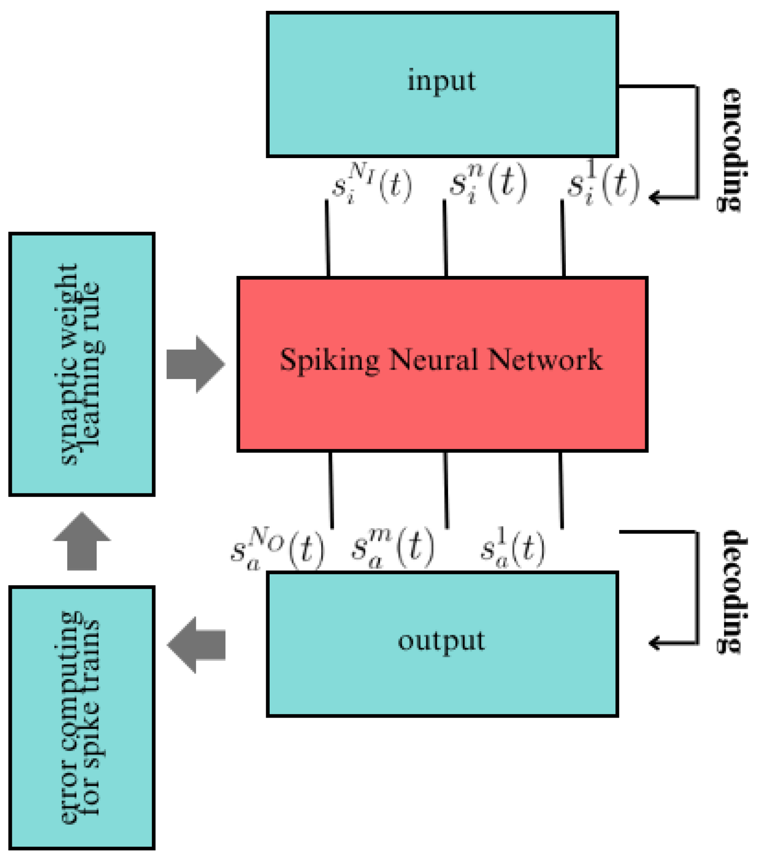
  • Representing the input data as spike trains, denoted as s i n S i , within the set of spike trains achieved through specific coding methods.
  • The spike trains s i n ( t ) are fed into the SNN, followed by employing a particular simulation strategy to execute the network. Consequently, the resultant output spike trains s m a S a within the set are obtained.
  • In accordance with the target output spike trains within the set s m a S a , the error function E ( S a , S d ) is computed, and subsequently, the synaptic weights are adjusted w w + Δ w .
  • Checking whether the error of the SNN, derived from the learning process, has reached a predefined minimum threshold or if the upper limit of learning epochs has been surpassed. If the termination condition is not met, the learning process is reiterated. Following supervised learning, the output spike trains S a from the network are decoded using a designated decoding methodology.

4.3.3. Training SNNs

To achieve high performance in neural networks, we primarily follow two routes: ANN-SNN conversion and direct training SNN from scratch.
  • ANN-SNN Conversion: exemplified by works such as [101,102], use ideas from artificial neural networks to transform ReLU activation into spike activation mechanisms, to enable the generation of SNNs. [103], for instance, identify maximum activation in the training dataset to facilitate direct module replacement for SNN conversion. In contrast, [104] employ a soft-reset mechanism and eliminate leakage during conversion, proving effective in achieving accurate conversions. [107] have further refined conversion techniques by decomposing conversion errors, adjusting bias terms, and introducing calibration methods. Although conversion yields fast and accurate results, achieving near-lossless conversion demands substantial time steps (>200) to accumulate spikes, potentially leading to increased latency. [?] suggest a conversion-based training approach employing a "soft reset" spiking neuron, termed the Residual Membrane Potential (RMP) spiking neuron, which closely emulates the functionality of the Rectified Linear Unit (ReLU). Unlike conventional "hard reset" mechanisms that reset the membrane potential to a fixed value at spiking instants, the RMP neuron maintains a "residual" potential above the firing threshold. This approach mitigates the loss of information typically encountered during the conversion from Artificial Neural Networks to Spiking Neural Networks (SNNs). Methods for converting ANNs to SNNs have achieved performance in deep SNNs that is comparable to that of the original ANNs. These methods offer a potential solution to the energy-efficiency challenges faced by ANNs during deployment ([105]).
  • Direct training of SNNs: as opposed to conversion methods, aims to reduce time steps and energy consumption by using gradient-descent algorithms. Notably, researchers have developed various strategies to address the non-differentiability of spike activation functions, akin to quantization or binarization neural networks ([106??], or adder neural networks ([107]. Achieving remarkable performance on datasets like CIFAR10, among others, has been demonstrated by works such as [108]. Some approaches resort to probabilistic models [109] or binary stochastic models ([110]) to approximate gradients, while others utilize rate-encoding networks ([111,112]) to quantify spike rate as information magnitude. For instance, [113] enhance the leaky integrate-and-fire (LIF) model to an iterative LIF model and introduce the STBP learning algorithm, while [114] propose the tdBN algorithm to balance gradient norms and smooth loss functions in SNN training, thus facilitating large-scale model optimization ([115]).

5. Methodology

Human design continues to be influential in defining three fundamental elements in Artificial Neural Networks: the learning objective, represented by an objective function (or loss function) aimed to be optimized or minimized; a collection of learning principles, articulated as updates to synaptic weights; and the network structure, delineated by pathways and connections facilitating information transmission (see Figure 16) ([116].) Within this framework, our focus isn’t on detailing the mechanics of computation, but rather on identifying the objective functions, learning principles, and architectures conducive to learning specific computations.
Several prominent behavioral and neurophysiological phenomena, such as grid cells, shape tuning, temporal receptive fields, visual illusions, and apparent model-based reasoning ([?]), have been observed to arise in deep Artificial Neural Networks (ANNs) trained on tasks akin to those encountered by animals ([117,118]). Additionally, several modeling studies suggest that concerns regarding the biological plausibility of end-to-end learning rules, such as those resembling the canonical error backpropagation algorithm, may be exaggerated. By taking advantage of relatively straightforward assumptions about cellular and subcellular electrophysiology, inhibitory microcircuits, spike timing patterns, short-term plasticity, and feedback connections, biological systems can potentially approximate backprop-like learning mechanisms in deep ANNs. Consequently, ANN-based models of the brain may not be as far-fetched as previously assumed and, simultaneously, demonstrate the capacity to clarify a substantial amount of neurobiological data.

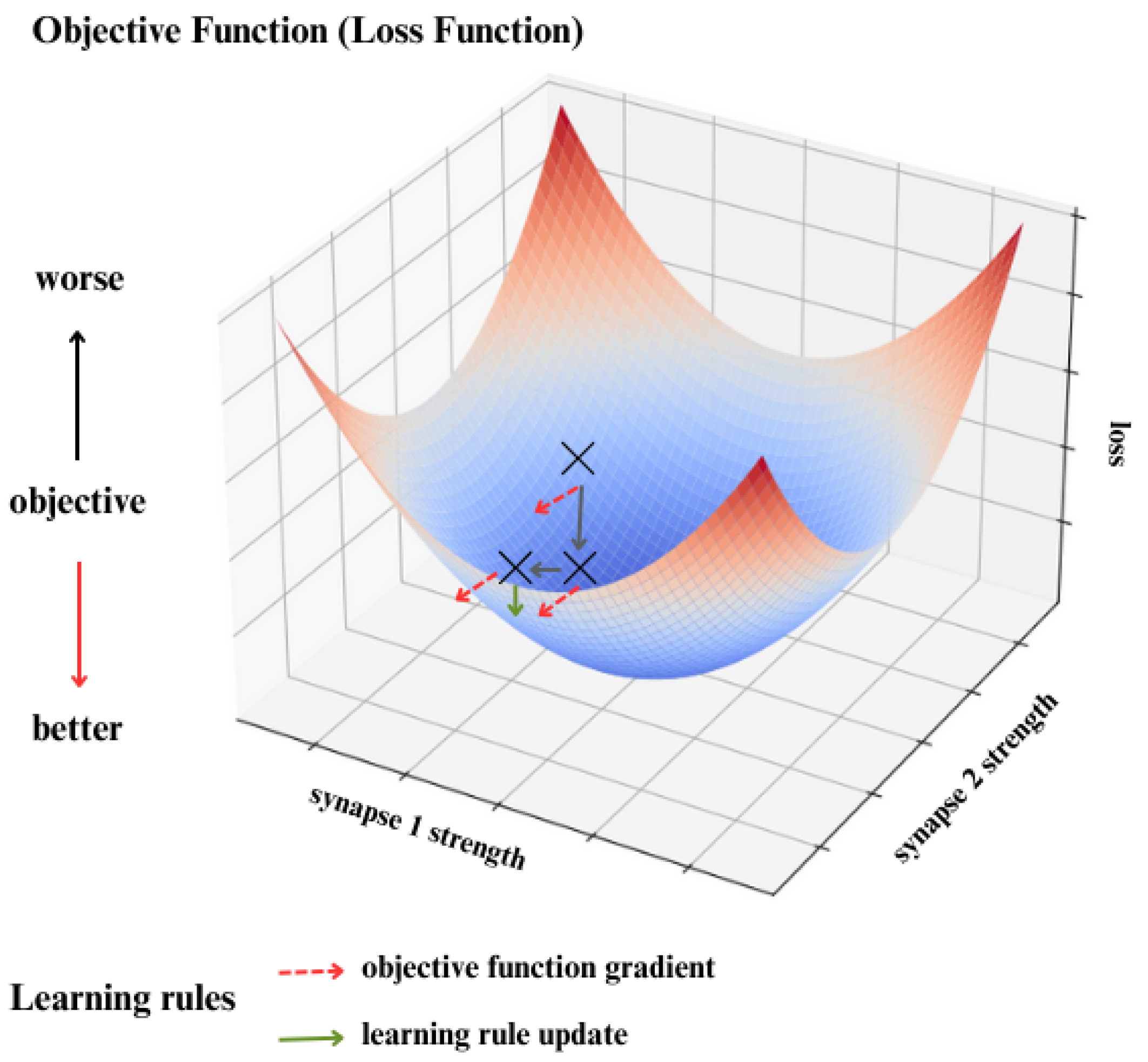
5.1. Objective Functions

Our comprehension of the foundational principles underlying Artificial Neural Networks is expanding, with indications suggesting their broad applicability. Simultaneously, advancements in our ability to monitor and manipulate extensive neural populations offer new avenues for testing hypotheses derived from deep learning literature. Predictive coding can be viewed as a mechanism aimed at minimizing the discrepancy between an input signal and a top-down prediction ([?]). In essence, by minimizing this error, predictive coding can be interpreted as diminishing the impact of external stimuli, akin to avoiding stimulation through prediction. [119] suggested that instead of optimizing a singular "end-to-end" cost function, the brain may optimize a range of internally generated cost functions tailored to specific brain functions. Backpropagation relies on the layered structure of the system to compute the sensitivity of the cost function to each weight. It starts by calculating the derivatives of the cost function with respect to the last layer, then propagates these derivatives backward to compute the derivatives for the preceding layers, and so on, until reaching the earliest layers. This method allows for smooth computation and maintains a consistent gradient estimate across all layers for a single input-output pattern. Consequently, deep and wide architectures with significant computational power can be trained efficiently using backpropagation.
In order to achieve biological learning with efficiency approaching that of machine learning methods, it is conceivable that more sophisticated gradient propagation mechanisms are necessary. Contrary to the once prevalent assumption, there are now numerous proposed "biologically plausible" mechanisms. These mechanisms offer potential alternatives for implementing optimization algorithms within neural circuits, similar to backpropagation, and which can efficiently use gradients ([119]).
To demonstrate the feasibility of learning with Backpropagation in such a network, [120] used a Spiking Neural Network composed of spiking neurons based on Gerstner’s spike response model. The architecture of [120]’s model was influenced by the structure proposed by [121], where each connection between a presynaptic and postsynaptic neuron incorporates multiple synapses, and neurons are constrained to emit a single spike. The learning algorithm introduced by [120], called SpikeProp, was devised along the lines of traditional neural network algorithms. Subsequently, it has been integrated into Spiking Neural Networks alongside various training techniques like backpropagation with momentum ([122]), QuickProp ([122]), resilient propagation (RProp) ([123]), and Levenberg-Marquardt backpropagation ([124]), all aimed at improving the efficiency of network training.
Since spike trains introduce the temporal component of Post-Synaptic Potential (PSP) induction, per-connection details are no longer necessary. While using many synapses, they serve as a generic case similar to biological neurons, improving the biological plausibility of learning using Spiking Neural Networks. The flexibility of synapse numbers, similar to the [125] model, might improve biological plausibility in SNN learning. [126] demonstrated the adaptability of the SpikeProp algorithm and its variants for recurrent architectures within Spiking Neural Networks. Their work demonstrated remarkable accuracy in classifying Poisson spike trains, even when subjected to noise interference.One limitation identified by [126] was that input neurons should not serve as postsynaptic neurons, while output neurons should not function as presynaptic neurons. In systems where traditional backpropagation isn’t feasible, alternative approaches are required. Weight perturbation is one such method, where gradients are estimated by perturbing synaptic weights and observing the resulting change in the objective function ([127]). Unlike backpropagation, weight perturbation doesn’t rely on understanding the functional relationship between the objective and the network weights ([128]). This makes it applicable to stochastic spiking networks and other systems where the underlying dynamics are complex or not fully understood ([129]).
The weight matrices of a neural network are initialized randomly or obtained from a pre-trained model. These matrices are multiplied with the input matrix (or the output from a previous layer) and passed through a nonlinear activation function to produce updated representations known as activations or feature maps. The loss function (also called objective function or empirical risk) measures the discrepancy between the network output and the known target data ([130]). Network weights are adjusted using stochastic gradient descent algorithms to minimize the loss function until the desired accuracy is achieved. Modern deep learning frameworks use reverse-mode automatic differentiation to compute the partial derivatives of the loss function with respect to each network parameter, enabling efficient back-propagation ([131]).
Common gradient descent algorithms like Stochastic Gradient Descent (SGD), Adam, and Adagrad are used for weight updates. Adaptive learning parameter tuning is employed by methods other than SGD. Different loss functions such as Binary Cross Entropy (BCE), Negative Log likelihood (NLLL), or Mean Squared Error (MSE) are chosen based on the specific task like classification or regression. Many Objective functions exist in the literature (See Table 1).

5.2. Learning Rules

In a classification problem, the underlying process that generates data defines the relationship between input attributes and output classes, known as the posterior probability distribution. This distribution indicates the probability that an object belongs to a specific class after observing relevant information. Bayesian classification theory ([135]) is based on posterior probability and is widely used in classification tasks. Neural networks can be employed to estimate an object’s posterior probabilities in classification problems. Accurately modeling the main data generation process relies on fitting the posterior probability distribution closely. This, in turn, maximizes the expected classifications,and optimizes classification accuracy. Therefore, if our goal is to develop classification models that accurately determine the group membership of unseen objects, our focus lies on how effectively the model approximates the underlying posterior probability distribution. Neural networks, with their ability to estimate posterior probabilities, can draw inferences and make judgments by using past experiences, allowing them to extrapolate this knowledge to similar future scenarios ([136]). If the neural and network dynamics, along with the objective function, are precisely known functions of the weights, then learning can be achieved by explicitly computing the corresponding gradients. However, the objective function in biological learning might be influenced by the dynamics of muscles and external variables in the environment that are not fully understood by the brain. Comparable complexities also exist in analog on-chip or robotic adaptations of machine learning ([137]). learning mechanisms are believed to use error signals, which represent the disparities between expected and observed spiking behaviors ([138,139]). Supervised learning, aims to minimize the disparity between actual and desired outputs. It has garnered significant attention in studies focusing on the cerebellum and cerebellar cortex within the central nervous system, although the precise mechanisms remain unclear ([140]). Supervised learning algorithms in Spiking Neural Networks can be broadly categorized into two approaches based on their strategies for reducing this disparity. One approach involves rigorous mathematical analyses to derive formulas for minimizing loss, while the other approach draws inspiration from biological mechanisms, such as the Widrow-Hoff rule ([141]) and the spike-timing dependent plasticity (STDP) rule ([142]). In the STDP rule, synaptic strength is reinforced when the presynaptic neuron fires before the postsynaptic neuron, and vice versa.
Starting from the differential equation of the leaky integrate-and-fire (LIF) neuron:
τ m d u d t = ( u ( t ) u rest ) + R m I ( t )
We integrate both sides of this equation with respect to time t over the time interval [ t p 1 , t p ] , where t p and t p 1 are the present and previous input spike times, respectively:
t p 1 t p τ m d u d t d t = t p 1 t p ( u ( t ) u rest ) + R m I ( t ) d t
Now, we’ll perform the integration on both sides:
τ m u ( t p 1 ) u ( t p ) d u = t p 1 t p ( u ( t ) u rest ) d t + R m t p 1 t p I ( t ) d t
τ m u ( t p ) u ( t p 1 ) = t p 1 t p u ( t ) d t u rest ( t p t p 1 ) + R m t p 1 t p I ( t ) d t
Now, we make use of the fact that the membrane potential is reset after each spike, so u ( t p 1 ) = u reset , and u ( t p ) = u ( t p ) :
τ m u ( t p ) u reset = t p 1 t p u ( t ) d t u rest ( t p t p 1 ) + R m t p 1 t p I ( t ) d t
Now, we’ll rearrange terms and divide both sides by τ m to isolate u ( t p ) :
u ( t p ) = u reset + 1 τ m u rest ( t p t p 1 ) t p 1 t p u ( t ) d t + R m t p 1 t p I ( t ) d t
We assume that the membrane potential changes slowly over the interval [ t p 1 , t p ] . This will allow us to approximate u ( t ) as approximately constant over this interval. So, we replace u ( t ) with u ( t p 1 ) throughout the interval. Then, we can approximate the integrals with step changes based on the timing of the spikes. which goes as follows:
u ( t p ) = u reset + 1 τ m u rest ( t p t p 1 ) u ( t p 1 ) ( t p t p 1 )
+ R m I ( t p ) ( t p t p 1 ) u ( t p ) = u reset + 1 τ m ( u rest u ( t p 1 ) ) ( t p t p 1 )
+ R m I ( t p ) ( t p t p 1 )
( t p t p 1 ) represents the time difference between two consecutive spikes, which we can call as Δ t . Also, u ( t p 1 ) is simply the membrane potential at the previous spike time t p 1 , which we call as u ( t p 1 ) = u .
So, the expression becomes:
u ( t p ) = u e Δ t τ m + 1 τ m u rest u + R m I ( t p ) Δ t
For a given input spike, the membrane potential u ( t p ) of a LIF neuron is updated using equation 33, where:
  • u ( t p ) is the membrane potential at time t p ,
  • u ( t p 1 ) is the membrane potential at the previous time step t p 1 ,
  • τ m is the membrane time constant,
  • u rest is the resting membrane potential,
  • R m is the membrane resistance,
  • I ( t p ) is the input current at time t p , and
  • Δ t is the time interval between consecutive input spikes t p and t p 1 .
Furthermore, a dynamic weight w dyn controls the refractory period as:
w dyn = 1 Δ t 2 if Δ t < T ref 1 otherwise
where:
  • Δ t = t out t p is the time difference between the latest output spike time t out and the present input spike time t p ,
  • T ref is the maximum duration of the refractory period.
U mp ( t p ) = U mp ( t p 1 ) e t p 1 t p τ mp + w i ( p ) W dyn
where:
  • w i ( p ) is the synaptic weight of the i-th synapse for the present p-th input spike,
  • W dyn is a dynamic weight controlling the refractory period.
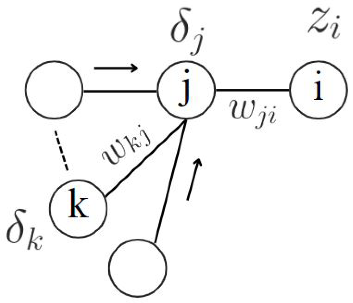
Thus, the impact of input spikes on u ( t p ) is inhibited for a brief period T r e f following an output spike. The dynamic weight W d y n gradually returns to 1 quadratically after the output spike at t o u t . Since W d y n is a global parameter of the neuron and applies uniformly to all synapses, it differs from short-term plasticity, which operates at the level of individual synapses. The rationale for using dynamic weights instead of simpler refractory mechanisms, such as directly blocking output spike generation, is that it enables the control of refractory states through external mechanisms. One example is the introduction of Winner-Take-All (WTA) circuits where lateral inhibition simultaneously puts all neurons competing in a WTA into the refractory state. This ensures that the winning neuron gets another chance to succeed in the competition, preventing other neurons from firing while only the winner needs to reset its membrane potential after generating a spike ([143]).
When u ( t p ) crosses the threshold value u t h , the LIF neuron generates an output spike, and u ( t p ) is decreased by the threshold amount:
u ( t p + ) = u ( t p ) u th
The time t p + represents the moment immediately following a membrane potential reset. A lower bound is established for the membrane potential at u th , and u m is truncated whenever it drops below this value. This approach helps to balance out the engagement of neurons during training by preventing them from reaching excessively negative membrane potentials.
[143] discovered that the accuracy of Spiking Neural Networks could be enhanced by using a competitive recurrent architecture, specifically by integrating Winner-Take-All (WTA) circuits into certain layers. In a WTA circuit, multiple neurons form a group with lateral inhibitory connections. Thus, when any neuron within the group emits an output spike, it suppresses the activity of all other neurons in the circuit, preventing them from spiking ([144,145]).
All lateral connections within a WTA circuit exhibit uniform strength, which reduces the memory and computational costs associated with their implementation. The level of lateral inhibition exerted on the membrane potential of a neuron is directly proportional to that neuron’s membrane potential threshold . With this approach, neurons with smaller membrane potential thresholds ( u t h ) experience weaker inhibition, while those with larger thresholds experience stronger inhibition. This contributes to better balance of neuronal activity during training, especially as neurons with higher activity tend to have larger membrane potential thresholds due to the threshold regularization schemes. Lateral inhibition is used to transition the dynamic weights of all inhibited neurons within a WTA circuit into a refractory state.The use of WTA circuits not only enhances classification accuracy, but also improves the stability and speed of convergence during training ([143]).
Neural networks are typically optimized using Stochastic Gradient Descent (SGD), where the vector of network parameters or weights w is updated by moving in the direction of the negative gradient of a loss function E, represented as
w = w η w E
where η is the learning rate. The backpropagation algorithm uses the chain rule to compute the partial derivatives w E . Here are the steps of the backpropagation process for conventional fully-connected spiking neural networks, involving weight updates based on computed gradients:
  • Compute the Derivative of E n with respect to w j i based on Equation 24:
    E n w j i = δ j z i
    where δ j is the error gradient for neuron j in layer l + 1 , and z i is the activation of neuron i in layer l.
  • Aggregate Gradients Across All Patterns:
    E w j i = n E n w j i
    = n ( δ j ( n ) z i ( n ) )
    where δ j ( n ) is the error gradient for neuron j in layer l + 1 for pattern n, and z i ( n ) is the activation of neuron i in layer l for pattern n.
  • Update the Parameters Using the Aggregated Gradients:
    w j i ( new ) = w j i ( old ) η E w j i
    where η is the learning rate, and E w j i is the total derivative of the error function E with respect to w j i .

5.3. Weight Initialization

There has been a lot of study into faster training algorithms since the Backpropagation, which is based on the steepest descent method, is sometimes deemed too slow for practical applications. Diverse methods have been investigated to accelerate convergence. One typical technique is to use more powerful optimization algorithms specifically designed for neural network learning. These algorithms are more efficient because they use advanced methods to modify training parameters ([146]). Another strategy uses heuristic techniques to optimize the convergence trajectory by dynamically adjusting the momentum term and learning rate. These methods can dramatically cut the number of iterations needed to satisfy convergence requirements by an order of magnitude or more. Another essential initial step in getting a neural network ready for training is weight initialization. The network’s weights are first established, then they are modified repeatedly as it the network learns, until the loss approaches zero. This produces an ideal weight matrix. As a result, weight initialization is extremely important in helping a network to converge during training. For effective end-to-end training, choosing a suitable weight initialization strategy is just as essential ([147]).
Two main methods for training deep networks: training from scratch and transfer learning—are shown in this table. Key resources, such as specialized hardware, and optimized libraries, are very important for improving efficiency and speeding up training for all approaches ([147]).
  • Training from Scratch: This method entails setting up the network and using optimization methods to train it. For effective calculation, this method makes use of GPUs, FPGAs, or TPUs in conjunction with optimized libraries like CUDA, cuDNN, MKL, and OpenCL.
  • Transfer Learning: Initializes and refines pre-trained models for use with certain tasks or datasets. This method works well for using previously learned characteristics and adjusting to fresh data.
Deep learning frameworks provide built-in functions for standard weight initialization methods and allow researchers to define custom weight initialization functions. When training a neural network from scratch, the network is initialized appropriately and then optimized using a suitable algorithm. Alternatively, transfer learning involves initializing a deep neural network with weights from a pre-trained model trained on a large dataset. In transfer learning, only the higher layers or all layers of the network are fine-tuned using a smaller new dataset, thus taking advantage of the learned features from the original dataset.
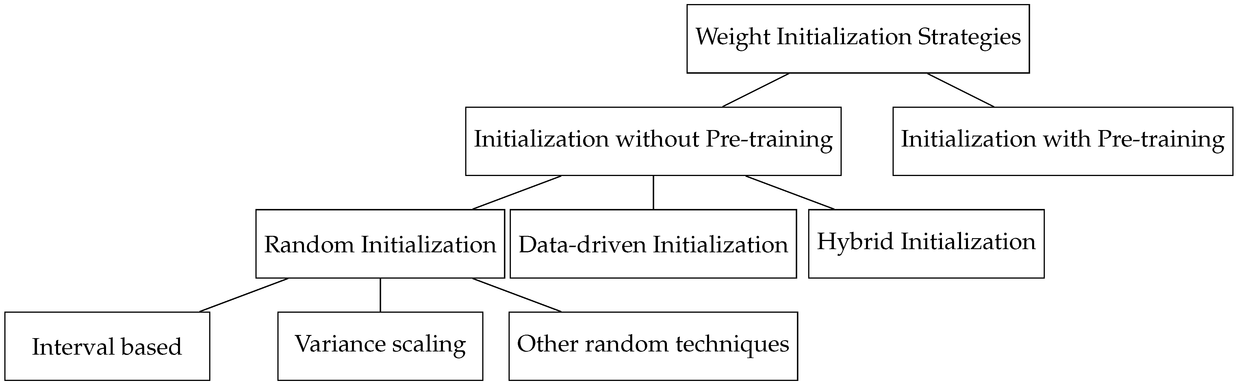
  • Initialization without pre-training:
    • Random initialization: This category investigates techniques that select weights from random distributions.
    • Interval based initialization: This category explores techniques that choose initial weights within an optimal derived range.
    • Variance scaling based initialization: This category examines various schemes where weights are scaled to maintain the variance of inputs and output activations.
    • Other: This category includes random initialization techniques not covered in interval-based or variance scaling approaches.
  • Data-driven initialization: This category focuses on initializing network weights derived from the training data.
  • Hybrid: This category explores techniques that combine random and data-driven initialization approaches.
  • Initialization with pre-training: This category explores methods where the initialization point is defined by an unsupervised approach for a supervised training algorithm ([147]).
These techniques are summarized in Figure 17. Table 2 categorizes different methodologies and emphasizes the major resources connected with each, laying down a perspective on the tools and technology required for efficient deep neural network training.
Weight initialization occurs before training begins. Weight initialization is typically performed to set initial values for the weights of a neural network before any training iterations take place. Common methods for weight initialization include random initialization ([148]), Xavier/Glorot initialization ([149]), He initialization ([150]).
  • Random Initialization: Initialize the weights w j i randomly from a specified distribution, for instance, uniform or normal distribution ([148]). For example:
    w j i ( initial ) Uniform ( a , b ) or w j i ( initial ) N ( μ , σ 2 )
    where a and b are the lower and upper bounds of the uniform distribution, and μ and σ 2 are the mean and variance of the normal distribution.
  • Xavier/Glorot Initialization: This method scales the initial weights based on the number of input and output neurons ([149]). For a uniform distribution:
    w j i ( initial ) Uniform 6 n in + n out , 6 n in + n out
    where n in is the number of input neurons and n out is the number of output neurons.
  • He Initialization: Similar to Xavier initialization, but optimized for ReLU activation functions ([150]):
    w j i ( initial ) Uniform 6 n in , 6 n in
    These initialization strategies set the starting values of weights w j i in the network and provide a good starting point for training. The choice of initialization method can significantly impact the convergence and performance of the neural network during training, thus it is important to carefully choose an initializing tactic.

5.4. Weight Regularization

As in conventional artificial neural networks, regularization techniques such as weight decay are essential for improving the generalization capability of spiking neural networks. Another challenge in training SNNs is that thresholds need to be initialized to large values, resulting in only a few neurons responding to input stimuli while many remain inactive. This is particularly problematic in Winner-Take-All (WTA) circuits.
Weight decay regularization is used to enhance the stability and generalization of SNNs. Specifically, we aim to maintain the condition defined by:
E i = 1 M l ( w j i l ) 2 = 1 or E ( w j i l ) 2 = 1 M l
Conventional L2-regularization has been found inadequate for this purpose because it leads to rapid initial weight growth followed by continued decrease. To address this issue, we introduce a new method called exponential regularization, inspired by max-norm regularization ([151]). The cost function for exponential regularization of neuron i in layer l is defined as:
E w ( l , i ) = 1 2 λ e β j = 1 M l ( w i j l ) 2 1
where β and λ are parameters that control the trade-off between error correction and regularization. The derivative of E w ( l , i ) with respect to a weight parameter is:
E w ( l , i ) w i j l = β λ · w i j l · e β j = 1 M ( l ) ( w i j l ) 2 1
where M l is the number of synapses of each neuron. L2-regularization has a constant rate of decay regardless of weight values, while max-norm regularization imposes an upper bound on weight increase. Exponential regularization is a compromise between the two: the decay rate is exponentially proportional to the sum of squared weights, effectively curbing weight increase like max-norm regularization. This approach ensures that weights consistently decay across a range of values, enhancing generalization similar to L2-regularization, while preventing excessive weight decrease by moderating the decay rate ([147]).

5.5. Weight Normalization

Before the introduction of batch normalization ([152]), the training time required for a network to converge was heavily reliant on meticulous hyperparameter initialization, such as setting initial weight values, and the use of learning rates, which extended the training duration. Moreover, the learning process was complicated by the interdependency of network layers, where minor adjustments in one layer could lead to amplified effects in subsequent layers. Batch normalization addresses these challenges by normalizing the inputs of each layer within the network, and not only just the input layer ([153]).
Following is the algorithm for Batch Normalization:
Algorithm 1: Batch Normalization
1:
Input:I (input to the batch normalization layer), γ (scaling), β (shifting), ϵ (numerical stability)
2:
Output:S (normalized output)
3:
// Compute batch statistics
4:
Compute μ I = mean ( I )
5:
Compute σ I 2 = variance ( I )
6:
// Normalize the input
7:
Initialize S as an empty array
8:
for each i in range(num_features) do
9:
    Compute d = σ I 2 [ i ] + ϵ
10:
    Compute S [ i ] = I [ i ] μ I [ i ] d
11:
end for
12:
// Scale and shift using γ and β
13:
Initialize S out as an empty array
14:
for each i in range(num_features) do
15:
    Compute S out [ i ] = γ [ i ] × S [ i ] + β [ i ]
16:
end for
17:
return S out

5.5.1. Threshold Regularization

Threshold regularization is used to balance the activities among N neurons that receive the same input stimuli, preventing the occurrence of excessive inactive neurons and improving accuracy. This regularization is particularly important for WTA circuits where neuron firing is suppressed by lateral inhibition.
During threshold regularization, when N w neurons fire after receiving an input spike, their thresholds are increased by ρ N Subsequently, for all N neurons, the threshold is decreased by ρ N w This adjustment makes highly active neurons less responsive to input stimuli due to increased thresholds, while rarely active neurons can respond more readily to subsequent stimuli.
Neurons with smaller thresholds are less influenced by negative inputs due to their tight lower bound in the range [ u th , u th ] . Threshold regularization actively prevents inactive neurons and encourages all neurons to contribute equally to optimization ([154]). This type of regularization has been utilized in competitive learning approaches ([155]).
To prevent excessive firing of neurons with very low thresholds, a lower threshold bound is established during training. If a neuron’s threshold is about to fall below this bound, all weight values of the neuron are uniformly increased. Threshold regularization is applied during forward propagation in training ([147]).
Finding the optimal combination of spiking thresholds, input weights, and input firing rates involves achieving a delicate balance. Higher spiking thresholds (or lower input weights) can reduce errors caused by excessive activation and suboptimal spike patterns, but they may increase errors due to insufficient activation ([156]). On the other hand, lower spiking thresholds (or higher input weights) can address under-activation issues but may introduce other errors. It’s important to note that the ratio of spiking threshold to input weights is very essential in determining how much evidence is integrated before a spike is fired, rather than focusing solely on their individual values.

6. Conclusion

As we conclude this study of the foundational constructs of Spiking Neural Networks (SNNs), we find ourselves in awe of the harmony that exists between nature’s mechanisms and the mathematical principles that govern them. These networks, modeled after the discrete spikes of biological neurons, represent an elegant mathematical framework for the efficient processing of time-varying information. The beauty of SNNs lies in their ability to reduce continuous, complex processes into discrete events, and their ability to concretize a new approach to computation that captures temporal dynamics with remarkable efficiency. The mathematical foundations of SNNs rest on the principles of timing and discrete event dynamics, a real departure from traditional continuous neural models. Traditional models, burdened by the inefficiencies of continuous data processing, are akin to rudimentary tools, sufficient for basic tasks but incapable of grasping the full complexity of dynamic systems. SNNs by contrast, operate with precision, using discrete spikes to mirror the time-based behavior of biological neurons. This foundational work lays the groundwork for future advancements in the field and opens a window to possibilities we have yet to fully imagine, where the intersection of biology and mathematics brings us closer to cracking the deepest mysteries of intelligence itself. As we continue to explore these new frontiers, we not only advance our understanding of artificial systems but also deepen our appreciation for the complex machinery that gave rise to the very minds capable of such discoveries.

References

  1. Wickens, A. A History of the Brain: From Stone Age surgery to modern neuroscience. Psychology Press. 2014. [Google Scholar] [CrossRef]
  2. Rocca, J. brain, 2019. [CrossRef]
  3. Gross, C. , History of Neuroscience: Early Neuroscience; 2017. [CrossRef]
  4. Persaud, T.; Loukas, M.; Tubbs, R. A History of Human Anatomy; Charles C. Thomas, Publisher, Limited, 2014.
  5. Green, C.D. Where did the ventricular localization of mental faculties come from? Journal of the history of the behavioral sciences 2003, 39 2, 131–42. [Google Scholar] [CrossRef]
  6. Mohammad, M., I. K.M.B.Q.M.A.M..A.A.
  7. Mazengenya, P.; Bhika, R. The Structure and Function of the Central Nervous System and Sense Organs in the Canon of Medicine by Avicenna. Archives of Iranian Medicine 2017, 20, 67–70. [Google Scholar] [PubMed]
  8. Sur, M.; Rubenstein, J. Patterning and Plasticity of the Cerebral Cortex. Science 2005, 310, 805–810. [Google Scholar] [CrossRef] [PubMed]
  9. Celesia, G. Alcmaeon of Croton’s Observations on Health, Brain, Mind, and Soul. Journal of the History of the Neurosciences 2012, 21, 409–426. [Google Scholar] [CrossRef]
  10. Benedum, J. [Importance of the brain in body-soul discussion from the history of medicine perspective]. Zentralblatt fur Neurochirurgie 1995, 56 4, 186–92. [Google Scholar]
  11. McCarley, R.; Hobson, J. The neurobiological origins of psychoanalytic dream theory. The American journal of psychiatry 1977, 134 11, 1211–21. [Google Scholar] [CrossRef]
  12. Kucewicz, M.; Cimbalnik, J.; Cimbalnik, J.; Matsumoto, J.; Brinkmann, B.; Bower, M.R.; Vasoli, V.; Sulc, V.; Sulc, V.; Meyer, F.; et al. High frequency oscillations are associated with cognitive processing in human recognition memory. Brain : a journal of neurology 2014, 137 Pt 8, 2231–44. [Google Scholar] [CrossRef] [PubMed]
  13. Herculano-Houzel, S. The remarkable, yet not extraordinary, human brain as a scaled-up primate brain and its associated cost. Proceedings of the National Academy of Sciences of the United States of America 2012, 109 Suppl 1, 10661–8. [Google Scholar] [CrossRef]
  14. Liu, S.C.; Delbruck, T. Neuromorphic sensory systems. Current Opinion in Neurobiology 2010, 20, 288–295. [Google Scholar] [CrossRef]
  15. Roy, K.; Jaiswal, A.R.; Panda, P. Towards spike-based machine intelligence with neuromorphic computing. Nature 2019, 575, 607–617. [Google Scholar] [CrossRef] [PubMed]
  16. Barney, N.; Lutkevich, B. What is neuromorphic computing?: Definition from TechTarget, 2023.
  17. van de Burgt, Y.; Melianas, A.; Keene, S.; Malliaras, G.; Salleo, A. Organic electronics for neuromorphic computing. Nature Electronics 2018, 1, 386–397. [Google Scholar] [CrossRef]
  18. Kempter, R.; Gerstner, W.; van Hemmen, J.V. Hebbian learning and spiking neurons. Physical Review E 1999, 59, 4498–4514. [Google Scholar] [CrossRef]
  19. Ma, D.; Shen, J.; Gu, Z.; Zhang, M.; Zhu, X.; Xu, X.; Xu, Q.; Shen, Y.; Pan, G. Darwin: A neuromorphic hardware co-processor based on spiking neural networks. Journal of Systems Architecture 2017, 77, 43–51. [Google Scholar] [CrossRef]
  20. Chen, G.; Cao, H.; Conradt, J.; Tang, H.; Rohrbein, F.; Knoll, A. Event-Based Neuromorphic Vision for Autonomous Driving: A Paradigm Shift for Bio-Inspired Visual Sensing and Perception. IEEE Signal Processing Magazine 2020, 37, 34–49. [Google Scholar] [CrossRef]
  21. Marković, D.; Mizrahi, A.; Querlioz, D.; Grollier, J. Physics for neuromorphic computing. Nature Reviews Physics 2020, 2, 499–510. [Google Scholar] [CrossRef]
  22. Brüderle, D.; Müller, E.; Davison, A.P.; Müller, E.B.; Schemmel, J.; Meier, K. Establishing a Novel Modeling Tool: A Python-Based Interface for a Neuromorphic Hardware System. Frontiers in Neuroinformatics 2008, 3. [Google Scholar] [CrossRef]
  23. Kim, C.H.; Lim, S.; Woo, S.; Kang, W.M.; Seo, Y.T.; Lee, S.; Lee, S.; Kwon, D.; Oh, S.; Noh, Y.; et al. Emerging memory technologies for neuromorphic computing. Nanotechnology 2018, 30. [Google Scholar] [CrossRef]
  24. Debat, G.; Chauhan, T.; Cottereau, B.; Masquelier, T.; Paindavoine, M.; Baurès, R. Event-Based Trajectory Prediction Using Spiking Neural Networks. Frontiers in Computational Neuroscience 2021, 15. [Google Scholar] [CrossRef]
  25. Kim, Y.; Panda, P. Optimizing Deeper Spiking Neural Networks for Dynamic Vision Sensing. Neural networks : the official journal of the International Neural Network Society 2021, 144, 686–698. [Google Scholar] [CrossRef]
  26. Wang, Y.; Du, B.; Shen, Y.; Wu, K.; Zhao, G.; Sun, J.; Wen, H. EV-Gait: Event-Based Robust Gait Recognition Using Dynamic Vision Sensors. 2019 IEEE/CVF Conference on Computer Vision and Pattern Recognition (CVPR) 2019, pp. 6351–6360. [CrossRef]
  27. Zhu, L.; Wang, X.; Chang, Y.; Li, J.; Huang, T.; Tian, Y. Event-based Video Reconstruction via Potential-assisted Spiking Neural Network. 2022 IEEE/CVF Conference on Computer Vision and Pattern Recognition (CVPR) 2022, pp. 3584–3594. [CrossRef]
  28. Wainberg, M.; Merico, D.; Delong, A.; Frey, B. Deep learning in biomedicine. Nature Biotechnology 2018, 36, 829–838. [Google Scholar] [CrossRef]
  29. Muzio, G.; O’Bray, L.; Borgwardt, K. Biological network analysis with deep learning. Briefings in Bioinformatics 2020, 22, 1515–1530. [Google Scholar] [CrossRef] [PubMed]
  30. Koumakis, L. Deep learning models in genomics; are we there yet? Computational and Structural Biotechnology Journal 2020, 18, 1466–1473. [Google Scholar] [CrossRef] [PubMed]
  31. Kumarasinghe, K.; Kasabov, N.; Taylor, D. Deep learning and deep knowledge representation in Spiking Neural Networks for Brain-Computer Interfaces. Neural networks : the official journal of the International Neural Network Society 2020, 121, 169–185. [Google Scholar] [CrossRef] [PubMed]
  32. Kirkland, P.; Clemente, C.; Macdonald, M.; Caterina, G.D.; Meoni, G. Neuromorphic Sensing and Processing for Space Domain Awareness. IGARSS 2023 - 2023 IEEE International Geoscience and Remote Sensing Symposium 2023, pp. 4738–4741. [CrossRef]
  33. Maass, W. Networks of spiking neurons: The third generation of neural network models. Neural Networks 1997, 10, 1659–1671. [Google Scholar] [CrossRef]
  34. Franck, R.; Masuy-Stroobant, G.; Lories, G.; Vaerenbergh, A.M.; Scheepers, P.; Verberk, G.; Felling, A.; Callatay, A.; Verleysen, M.; Peeters, D.; et al. The Explanatory Power of Models, Bridging the Gap between Empirical and Theoretical Research in the Social Sciences; 2002. [CrossRef]
  35. McCulloch, W.S.; Pitts, W. A logical calculus of the ideas immanent in nervous activity. Bulletin of Mathematical Biophysics 1943, 5, 115–133. [Google Scholar] [CrossRef]
  36. Tavanaei, A.; Ghodrati, M.; Kheradpisheh, S.R.; Masquelier, T.; Maida, A. Deep Learning in Spiking Neural Networks. Neural networks : the official journal of the International Neural Network Society 2018, 111, 47–63. [Google Scholar] [CrossRef]
  37. Ghosh-Dastidar, S.; Adeli, H. Spiking Neural Networks. Int. J. Neural Syst. 2009, 19, 295–308. [Google Scholar] [CrossRef]
  38. Maass, W. To Spike or Not to Spike: That Is the Question. Proc. IEEE 2015, 103, 2219–2224. [Google Scholar] [CrossRef]
  39. Maass, W. Lower bounds for the computational power of networks of spiking neurons. Neural Comput. 1996, 8, 1–40. [Google Scholar] [CrossRef]
  40. Gerstner, W.; Kistler, W.M.; Naud, R.; Paninski, L. Neuronal Dynamics: From Single Neurons to Networks and Models of Cognition; Cambridge University Press, 2014.
  41. Ramón y Cajal, S. Histologie du système nerveux de l’homme & des vertébrés; Vol. v. 1, Paris, Maloine, 1909-11; p. 1012. https://www.biodiversitylibrary.org/bibliography/48637.
  42. Völgyi, K.; Gulyássy, P.; Háden, K.; Kis, V.; Badics, K.; Kékesi, K.; Simor, A.; Győrffy, B.; Toth, E.; Lubec, G.; et al. Synaptic mitochondria: a brain mitochondria cluster with a specific proteome. Journal of proteomics 2015, 120, 142–57. [Google Scholar] [CrossRef] [PubMed]
  43. Carrillo, S.; Harkin, J.; McDaid, L.; Pande, S.; Cawley, S.; McGinley, B.; Morgan, F. Advancing Interconnect Density for Spiking Neural Network Hardware Implementations using Traffic-Aware Adaptive Network-on-Chip Routers. Neural Networks 2012, 33, 42–57. [Google Scholar] [CrossRef]
  44. Ferrante, M.A. Chapter 10 - Neuromuscular electrodiagnosis. In Motor System Disorders, Part I: Normal Physiology and Function and Neuromuscular Disorders; Younger, D.S., Ed.; Elsevier, 2023; Vol. 195, Handbook of Clinical Neurology, pp. 251–270. [CrossRef]
  45. Connors, B.; Long, M.A. Electrical synapses in the mammalian brain. Annual review of neuroscience 2004, 27, 393–418. [Google Scholar] [CrossRef] [PubMed]
  46. Häusser, M. Synaptic function: Dendritic democracy. Current Biology 2001, 11, R10–R12. [Google Scholar] [CrossRef] [PubMed]
  47. Peters, A.; Palay, S. The morphology of synapses. Journal of Neurocytology 1996, 25, 687–700. [Google Scholar] [CrossRef]
  48. Haydon, P. Glia: listening and talking to the synapse. Nature Reviews Neuroscience 2001, 2, 185–193. [Google Scholar] [CrossRef]
  49. Brette, R.; Gerstner, W. Adaptive exponential integrate-and-fire model as an effective description of neuronal activity. Journal of neurophysiology 2005, 94 5, 3637–42. [Google Scholar] [CrossRef]
  50. Hansel, D.; Mato, G.; Meunier, C.; Neltner, L. On Numerical Simulations of Integrate-and-Fire Neural Networks. Neural Computation 1998, 10, 467–483. [Google Scholar] [CrossRef]
  51. Ghosh-Dastidar, S.; Adeli, H. A new supervised learning algorithm for multiple spiking neural networks with application in epilepsy and seizure detection. Neural networks : the official journal of the International Neural Network Society 2009, 22 10, 1419–31.
  52. Brunel, N.; van Rossum, M. Quantitative investigations of electrical nerve excitation treated as polarization: Louis Lapicque 1907 · Translated by:. Biological Cybernetics 2007, 97, 341–349. [Google Scholar] [CrossRef]
  53. Hill, A.V. Excitation and Accommodation in Nerve. Proceedings of The Royal Society B: Biological Sciences 1936, 119, 305–355. [Google Scholar]
  54. Burkitt, A. A Review of the Integrate-and-fire Neuron Model: I. Homogeneous Synaptic Input. Biological Cybernetics 2006, 95, 1–19. [Google Scholar] [CrossRef] [PubMed]
  55. Gerstein, G.L.; Mandelbrot, B.B. RANDOM WALK MODELS FOR THE SPIKE ACTIVITY OF A SINGLE NEURON. Biophysical journal 1964, 4, 41–68. [Google Scholar] [CrossRef] [PubMed]
  56. Uhlenbeck, G.E.; Ornstein, L.S. On the Theory of the Brownian Motion. Phys. Rev. 1930, 36, 823–841. [Google Scholar] [CrossRef]
  57. Knight, B.W. Dynamics of Encoding in a Population of Neurons. The Journal of General Physiology 1972, 59, 734–766. [Google Scholar] [CrossRef] [PubMed]
  58. Kryukov, V.I. Wald’s Identity and Random Walk Models for Neuron Firing. Advances in Applied Probability 1976, 8, 257–277. [Google Scholar] [CrossRef]
  59. Tuckwell, H. On stochastic models of the activity of single neurons. Journal of Theoretical Biology - J THEOR BIOL 1977, 65, 783–785. [Google Scholar] [CrossRef]
  60. An analysis of Stein’s model for stochastic neuronal excitation. Biological cybernetics 1982, 45, 107–114. [CrossRef]
  61. Lánský, P. On approximations of Stein’s neuronal model. Journal of Theoretical Biology 1984, 107, 631–647. [Google Scholar] [CrossRef]
  62. Al, H.; Af, H. A quantitative description of membrane current and its application to conduction and excitation in nerve. Bulletin of Mathematical Biology 1952, 52, 25–71. [Google Scholar]
  63. Li, M.; Tsien, J.Z. Neural code-Neural Self-information Theory on how cell-assembly code rises from spike time and neuronal variability. Front. Cell. Neurosci. 2017, 11, 236. [Google Scholar] [CrossRef]
  64. Gerstner, W.; Kreiter, A.K.; Markram, H.; Herz, A.V. Neural codes: firing rates and beyond. Proc. Natl. Acad. Sci. U. S. A. 1997, 94, 12740–12741. [Google Scholar] [CrossRef] [PubMed]
  65. Azarfar, A.; Calcini, N.; Huang, C.; Zeldenrust, F.; Celikel, T. Neural coding: A single neuron’s perspective. Neurosci. Biobehav. Rev. 2018, 94, 238–247. [Google Scholar] [CrossRef] [PubMed]
  66. Adrian, E.D.; Zotterman, Y. The impulses produced by sensory nerve endings. J. Physiol. 1926, 61, 465–483. [Google Scholar] [CrossRef]
  67. Johansson, R.S.; Birznieks, I. First spikes in ensembles of human tactile afferents code complex spatial fingertip events. Nat. Neurosci. 2004, 7, 170–177. [Google Scholar] [CrossRef]
  68. Ponulak, F.; Kasinski, A. Introduction to spiking neural networks: Information processing, learning and applications. Acta Neurobiol. Exp. (Wars.) 2011, 71, 409–433. [Google Scholar] [CrossRef]
  69. O’Keefe, J.; Recce, M.L. Phase relationship between hippocampal place units and the EEG theta rhythm. Hippocampus 1993, 3, 317–330. [Google Scholar] [CrossRef]
  70. Zeldenrust, F.; Wadman, W.J.; Englitz, B. Neural coding with bursts—current state and future perspectives. Front. Comput. Neurosci. 2018, 12. [Google Scholar] [CrossRef]
  71. Buonomano, D.V.; Merzenich, M.M. Cortical plasticity: from synapses to maps. Annual review of neuroscience 1998, 21, 149–86. [Google Scholar] [CrossRef]
  72. Karmarkar, U.; Dan, Y. Experience-Dependent Plasticity in Adult Visual Cortex. Neuron 2006, 52, 577–85. [Google Scholar] [CrossRef]
  73. Caporale, N.; Dan, Y. Spike timing-dependent plasticity: a Hebbian learning rule. Annual review of neuroscience 2008, 31, 25–46. [Google Scholar] [CrossRef]
  74. Hebb, D. O. The organization of behavior: A neuropsychological theory. New York: John Wiley and Sons, Inc., 1949. 335 p. $4.00. Sci. Educ. 1950, 34, 336–337. [Google Scholar]
  75. Bliss, T.V.P.; Gardner-Medwin, A.R. Long-lasting potentiation of synaptic transmission in the dentate area of the unanaesthetized rabbit following stimulation of the perforant path. The Journal of Physiology 1973, 232. [Google Scholar] [CrossRef] [PubMed]
  76. Artola, A.; Singer, W. Long-term depression of excitatory synaptic transmission and its relationship to long-term potentiation. Trends in Neurosciences 1993, 16, 480–487. [Google Scholar] [CrossRef]
  77. Artola, A.; Singer, W. Artola, A. & Singer, W. Long-term potentiation and NMDA receptors in rat visual cortex. Nature 330, 649-652. Nature 1987, 330, 649–52. [Google Scholar] [CrossRef]
  78. Dudek, S.M.; Bear, M.F. Bidirectional long-term modification of synaptic effectiveness in the adult and immature hippocampus. J. Neurosci. 1993, 13, 2910–2918. [Google Scholar] [CrossRef]
  79. Kirkwood, A.; Bear, M.F. Hebbian synapses in visual cortex. J. Neurosci. 1994, 14, 1634–1645. [Google Scholar] [CrossRef]
  80. Bliss, T.V.; Collingridge, G.L. A synaptic model of memory: long-term potentiation in the hippocampus. Nature 1993, 361, 31–39. [Google Scholar] [CrossRef]
  81. Montemurro, M.; Rasch, M.; Murayama, Y.; Logothetis, N.; Panzeri, S. Phase-of-Firing Coding of Natural Visual Stimuli in Primary Visual Cortex. Current Biology 2008, 18, 375–380. [Google Scholar] [CrossRef]
  82. Lopour, B.A.; Tavassoli, A.; Fried, I.; Ringach, D. Coding of Information in the Phase of Local Field Potentials within Human Medial Temporal Lobe. Neuron 2013, 79, 594–606. [Google Scholar] [CrossRef]
  83. Averbeck, B.; Latham, P.; Pouget, A. Neural correlations, population coding and computation. Nature Reviews Neuroscience 2006, 7, 358–366. [Google Scholar] [CrossRef]
  84. Izhikevich, E.M.; Desai, N.S.; Walcott, E.C.; Hoppensteadt, F.C. Bursts as a unit of neural information: selective communication via resonance. Trends Neurosci. 2003, 26, 161–167. [Google Scholar] [CrossRef] [PubMed]
  85. Eyherabide, H.G.; Rokem, A.; Herz, A.V.M.; Samengo, I. Bursts generate a non-reducible spike-pattern code. Front. Neurosci. 2009, 3, 8–14. [Google Scholar] [CrossRef]
  86. Guo, W.; Fouda, M.E.; Eltawil, A.M.; Salama, K.N. Neural Coding in Spiking Neural Networks: A Comparative Study for Robust Neuromorphic Systems. Frontiers in Neuroscience 2021, 15. [Google Scholar] [CrossRef] [PubMed]
  87. .
  88. Markram, H.; Gerstner, W.; Sjöström, P.J. A History of Spike-Timing-Dependent Plasticity. Frontiers in Synaptic Neuroscience 2011, 3. [Google Scholar] [CrossRef]
  89. Markram, H.; Lübke, J.; Frotscher, M.; Sakmann, B. Regulation of Synaptic Efficacy by Coincidence of Postsynaptic APs and EPSPs. Science (New York, N.Y.) 1997, 275, 213–5. [Google Scholar] [CrossRef]
  90. qiang Bi, G.; ming Poo, M. Synaptic Modifications in Cultured Hippocampal Neurons: Dependence on Spike Timing, Synaptic Strength, and Postsynaptic Cell Type. Journal of Neuroscience 1998, 18, 10464–10472, [https://www.jneurosci.org/content/18/24/10464.full.pdf]. [Google Scholar] [CrossRef]
  91. Nelson, S.; Sjöström, P.; Turrigiano, G. Rate and timing in cortical synaptic plasticity. Philosophical transactions of the Royal Society of London. Series B, Biological sciences 2003, 357, 1851–7. [Google Scholar] [CrossRef]
  92. Rao, R.; Olshausen, B.; Lewicki, M. Probabilistic Models of the Brain: Perception and Neural Function 2002.
  93. Doya, K.; Ishii, S.; Pouget, A.; Rao, R.P.N. Bayesian Brain: Probabilistic Approaches to Neural Coding; The MIT Press, 2007.
  94. Kording, K.; Wolpert, D. Bayesian integration in sensorimotor learning. Nature 2004, 427, 244–7. [Google Scholar] [CrossRef]
  95. Nessler, B.; Pfeiffer, M.; Maass, W. STDP enables spiking neurons to detect hidden causes of their inputs. In Proceedings of the Proc. of Advances in Neural Information Processing Systems (NIPS). MIT Press, 2010, pp. 1357–1365. 23rd Advances in Neural Information Processing Systems ; Conference date: 08-12-2009 Through 12-12-2009.
  96. Nessler, B.; Pfeiffer, M.; Buesing, L.; Maass, W. Bayesian Computation Emerges in Generic Cortical Microcircuits through Spike-Timing-Dependent Plasticity. PLOS Computational Biology 2013, 9, 1–30. [Google Scholar] [CrossRef]
  97. Klampfl, S.; Maass, W. Emergence of Dynamic Memory Traces in Cortical Microcircuit Models through STDP. Journal of Neuroscience 2013, 33, 11515–11529, [https://www.jneurosci.org/content/33/28/11515.full.pdf]. [Google Scholar] [CrossRef]
  98. Bishop, C. Neural Networks For Pattern Recognition; Vol. 227, 2005. [CrossRef]
  99. Youngeun, K.; Priyadarshini, P. Visual explanations from spiking neural networks using inter-spike intervals. Sci. Rep. 2021, 11, 19037. [Google Scholar]
  100. Wang, X.; Lin, X.; Dang, X. Supervised learning in spiking neural networks: A review of algorithms and evaluations. Neural Networks 2020, 125, 258–280. [Google Scholar] [CrossRef] [PubMed]
  101. Han, B.; Srinivasan, G.; Roy, K. RMP-SNN: Residual Membrane Potential Neuron for Enabling Deeper High-Accuracy and Low-Latency Spiking Neural Network. 06 2020, pp. 13555–13564. [CrossRef]
  102. Sengupta, A.; Ye, Y.; Wang, R.; Liu, C.; Roy, K. Going Deeper in Spiking Neural Networks: VGG and Residual Architectures. Frontiers in Neuroscience 2018, 13. [Google Scholar] [CrossRef] [PubMed]
  103. Rueckauer, B.; Lungu, I.A.; Hu, Y.; Pfeiffer, M. Theory and tools for the conversion of analog to spiking convolutional neural networks 2016.
  104. Han, B.; Roy, K. , Deep Spiking Neural Network: Energy Efficiency Through Time Based Coding; 2020; pp. 388–404. [CrossRef]
  105. Yamazaki, K.; Vo-Ho, V.K.; Bulsara, D.; Le, N. Spiking neural networks and their applications: A review. Brain Sci. 2022, 12, 863. [Google Scholar] [CrossRef]
  106. Li, Y.; Dong, X.; Wang, W. Additive Powers-of-Two quantization: An efficient non-uniform discretization for neural networks 2019. arXiv:cs.LG/1909.13144.
  107. Chen, H.; Wang, Y.; Xu, C.; Shi, B.; Xu, C.; Tian, Q.; Xu, C. AdderNet: Do we really need multiplications in deep learning? 2019. arXiv:cs.CV/1912.13200.
  108. Amir, A.; Taba, B.; Berg, D.; Melano, T.; McKinstry, J.; Di Nolfo, C.; Nayak, T.; Andreopoulos, A.; Garreau, G.; Mendoza, M.; et al. A Low Power, Fully Event-Based Gesture Recognition System. In Proceedings of the 2017 IEEE Conference on Computer Vision and Pattern Recognition (CVPR); 2017; pp. 7388–7397. [Google Scholar] [CrossRef]
  109. Brea, J.; Senn, W.; Pfister, J.P. Matching Recall and Storage in Sequence Learning with Spiking Neural Networks. Journal of Neuroscience 2013, 33, 9565–9575, [https://www.jneurosci.org/content/33/23/9565.full.pdf]. [Google Scholar] [CrossRef]
  110. Bengio, Y.; Léonard, N.; Courville, A. Estimating or propagating gradients through stochastic neurons for conditional computation 2013. [arXiv:cs.LG/1308.3432]. arXiv:cs.LG/1308.3432.
  111. Lee, J.H.; Delbruck, T.; Pfeiffer, M. Training deep spiking neural networks using backpropagation 2016. [arXiv:cs.NE/1608.08782]. arXiv:cs.NE/1608.08782.
  112. Neftci, E.; Augustine, C.; Paul, S.; Detorakis, G. Event-Driven Random Back-Propagation: Enabling Neuromorphic Deep Learning Machines. Frontiers in Neuroscience 2017, 11. [Google Scholar] [CrossRef]
  113. Wu, Y.; Deng, L.; Li, G.; Zhu, J.; Shi, L. Spatio-Temporal Backpropagation for Training High-Performance Spiking Neural Networks. Frontiers in Neuroscience 2017, 12. [Google Scholar] [CrossRef]
  114. Zheng, H.; Wu, Y.; Deng, L.; Hu, Y.; Li, G. Going deeper with directly-trained larger spiking neural networks 2020. [arXiv:cs.NE/2011.05280]. arXiv:cs.NE/2011.05280.
  115. Li, Y.; Guo, Y.; Zhang, S.; Deng, S.; Hai, Y.; Gu, S. Differentiable Spike: Rethinking Gradient-Descent for Training Spiking Neural Networks. In Proceedings of the Advances in Neural Information Processing Systems; Ranzato, M.; Beygelzimer, A.; Dauphin, Y.; Liang, P.; Vaughan, J.W., Eds. Curran Associates, Inc., 2021, Vol. 34, pp. 23426–23439.
  116. Goodfellow, I.; Bengio, Y.; Courville, A. Deep Learning; MIT Press, 2016. http://www.deeplearningbook.org.
  117. Kell, A.; Yamins, D.; Shook, E.; Norman-Haignere, S.; McDermott, J. A Task-Optimized Neural Network Replicates Human Auditory Behavior, Predicts Brain Responses, and Reveals a Cortical Processing Hierarchy. Neuron 2018, 98. [Google Scholar] [CrossRef]
  118. Bashivan, P.; Kar, K.; Dicarlo, J. Neural population control via deep image synthesis. Science 2019, 364, eaav9436. [Google Scholar] [CrossRef]
  119. .
  120. Bohte, S.M.; Kok, J.N.; La Poutré, H. Error-backpropagation in temporally encoded networks of spiking neurons. Neurocomputing 2002, 48, 17–37. [Google Scholar] [CrossRef]
  121. Natschläger, T.; Ruf, B. Pattern analysis with spiking neurons using delay coding. Neurocomputing 1999, 26-27, 463–469. [Google Scholar] [CrossRef]
  122. Xin, J.; Embrechts, M. Supervised learning with spiking neural networks. 02 2001, Vol. 3, pp. 1772 – 1777 vol.3. [CrossRef]
  123. McKennoch, S.; Liu, D.; Bushnell, L. Fast Modifications of the SpikeProp Algorithm. 01 2006, Vol. 16, pp. 3970 – 3977. [CrossRef]
  124. Silva, S.; Ruano, A. Application of Levenberg-Marquardt method to the training of spiking neural networks. 11 2005, Vol. 3, pp. 1354– 1358. [CrossRef]
  125. Schrauwen, B.; Campenhout, J. Extending SpikeProp. 08 2004, Vol. 1, p. 475. [CrossRef]
  126. Booij, O.; Nguyen, H. A gradient descent rule for spiking neurons emitting multiple spikes. Information Processing Letters 2005, 95, 552–558. [Google Scholar] [CrossRef]
  127. Fiete, I.R.; Seung, H.S. Gradient learning in spiking neural networks by dynamic perturbation of conductances. Physical review letters 2006, 97 4, 048104. [Google Scholar] [CrossRef]
  128. Dembo, A.; Kailath, T. Model-free distributed learning. IEEE Transactions on Neural Networks 1990, 1, 58–70. [Google Scholar] [CrossRef] [PubMed]
  129. Vieira, J.; Arévalo, O.; Pawelzik, K. Stochastic gradient ascent learning with spike timing dependent plasticity. BMC Neuroscience 2011, 12, P250. [Google Scholar] [CrossRef]
  130. Choudhary, K.; DeCost, B.; Chen, C.; Jain, A.; Tavazza, F.; Cohn, R.; Park, C.W.; Choudhary, A.; Agrawal, A.; Billinge, S.J.L.; et al. Recent advances and applications of deep learning methods in materials science. Npj Comput. Mater. 2022, 8. [Google Scholar] [CrossRef]
  131. Baydin, A.G.; Pearlmutter, B.A.; Radul, A.A.; Siskind, J.M. Automatic differentiation in machine learning: a survey. Journal of machine learning research 2018, 18, 1–43. [Google Scholar]
  132. Jadon, A.; Patil, A.; Jadon, S. A comprehensive survey of regression based loss functions for time Series Forecasting 2022. [arXiv:cs.LG/2211.02989]. arXiv:cs.LG/2211.02989.
  133. Zhang, Z.; Sabuncu, M.R. Generalized cross entropy loss for training deep neural networks with noisy labels 2018. [arXiv:cs.LG/1805.07836]. arXiv:cs.LG/1805.07836.
  134. Rosset, S.; Zhu, J.; Hastie, T. Margin maximizing loss functions. In Proceedings of the Proceedings of the 16th International Conference on Neural Information Processing Systems, Cambridge, MA, USA, 2003; NIPS’03, p. 1237–1244.
  135. Duda, R.O.; Hart, P.E. Pattern classification and scene analysis. In Proceedings of the A Wiley-Interscience publication; 1974. [Google Scholar]
  136. Kline, D.M.; Berardi, V.L. Revisiting squared-error and cross-entropy functions for training neural network classifiers. Neural Computing & Applications 2005, 14, 310–318. [Google Scholar] [CrossRef]
  137. Fiete, I.; Seung, H. Gradient learning in spiking neural networks by dynamic perturbation of conductances. Physical review letters 2006, 97 4, 048104. [Google Scholar] [CrossRef]
  138. Wu, J.; Yılmaz, E.; Zhang, M.; Li, H.; Tan, K.C. Deep Spiking Neural Networks for Large Vocabulary Automatic Speech Recognition. Frontiers in Neuroscience 2020, 14. [Google Scholar] [CrossRef]
  139. Bastos, A.M.; Usrey, W.; Adams, R.A.; Mangun, G.R.; Fries, P.; Friston, K.J. Canonical Microcircuits for Predictive Coding. Neuron 2012, 76, 695–711. [Google Scholar] [CrossRef] [PubMed]
  140. Luo, X.; Qu, H.; Zhang, Y.; Chen, Y. First Error-Based Supervised Learning Algorithm for Spiking Neural Networks. Frontiers in Neuroscience 2019, 13. [Google Scholar] [CrossRef] [PubMed]
  141. Widrow, B.; Lehr, M. 30 years of adaptive neural networks: perceptron, Madaline, and backpropagation. Proceedings of the IEEE 1990, 78, 1415–1442. [Google Scholar] [CrossRef]
  142. Masquelier, T.; Guyonneau, R.; Thorpe, S. Competitive STDP-Based Spike Pattern Learning. Neural computation 2009, 21, 1259–76. [Google Scholar] [CrossRef] [PubMed]
  143. Lee, J.; Delbrück, T.; Pfeiffer, M. Training Deep Spiking Neural Networks Using Backpropagation. Frontiers in Neuroscience 2016, 10. [Google Scholar] [CrossRef]
  144. Rozell, C.J.; Johnson, D.H.; Baraniuk, R.G.; Olshausen, B.A. Sparse coding via thresholding and local competition in neural circuits. Neural Comput. 2008, 20, 2526–2563. [Google Scholar] [CrossRef]
  145. Fair, K.L.; Mendat, D.R.; Andreou, A.G.; Rozell, C.J.; Romberg, J.; Anderson, D.V. Sparse Coding Using the Locally Competitive Algorithm on the TrueNorth Neurosynaptic System. Frontiers in Neuroscience 2019, 13. [Google Scholar] [CrossRef]
  146. Yam, J.Y.F.; Chow, T.; Leung, C. A new method in determining initial weights of feedforward neural networks for training enhancement. Neurocomputing 1997, 16, 23–32. [Google Scholar] [CrossRef]
  147. Narkhede, M.V.; Bartakke, P.; Sutaone, M. A review on weight initialization strategies for neural networks. Artificial Intelligence Review 2021, 55, 291–322. [Google Scholar] [CrossRef]
  148. Sussillo, D.; Abbott, L.F. Random Walk Initialization for Training Very Deep Feedforward Networks. arXiv: Neural and Evolutionary Computing 2014.
  149. Glorot, X.; Bengio, Y. Understanding the difficulty of training deep feedforward neural networks. In Proceedings of the Proceedings of the Thirteenth International Conference on Artificial Intelligence and Statistics; Teh, Y.W.; Titterington, M., Eds., Chia Laguna Resort, Sardinia, Italy, 13–15 May 2010; Vol. 9, Proceedings of Machine Learning Research, pp. 249–256.
  150. He, K.; Zhang, X.; Ren, S.; Sun, J. Delving deep into rectifiers: Surpassing human-level performance on ImageNet classification 2015. arXiv:cs.CV/1502.01852.
  151. Srivastava, N.; Hinton, G.; Krizhevsky, A.; Sutskever, I.; Salakhutdinov, R. Dropout: A Simple Way to Prevent Neural Networks from Overfitting. Journal of Machine Learning Research 2014, 15, 1929–1958. [Google Scholar]
  152. Ioffe, S.; Szegedy, C. Batch Normalization: Accelerating Deep Network Training by Reducing Internal Covariate Shift 2015.
  153. Garbin, C.; Zhu, X.; Marques, O. Dropout vs. batch normalization: an empirical study of their impact to deep learning. Multimedia Tools and Applications 2020, 79, 12777–12815. [Google Scholar] [CrossRef]
  154. Afshar, S.; George, L.; Tapson, J.; van Schaik, A.; Chazal, P.; Hamilton, T. Turn Down that Noise: Synaptic Encoding of Afferent SNR in a Single Spiking Neuron. IEEE transactions on biomedical circuits and systems 2014, 9. [Google Scholar] [CrossRef] [PubMed]
  155. Rumelhart, D.E.; Zipser, D. Feature discovery by Competitive Learning. Cogn. Sci. 1985, 9, 75–112. [Google Scholar]
  156. Diehl, P.U.; Neil, D.; Binas, J.; Cook, M.; Liu, S.C.; Pfeiffer, M. Fast-classifying, high-accuracy spiking deep networks through weight and threshold balancing. In Proceedings of the 2015 International Joint Conference on Neural Networks (IJCNN); 2015; pp. 1–8. [Google Scholar] [CrossRef]
Figure 1. Neuromorphic computing mimics the architecture and functionality of the human brain, while von Neumann architecture, typical of traditional computers, separates memory and processing units ([16]).
Preprints 145617 g001
Figure 2. Illustration of the famous McCulloch and Pitts model of 1943 ([35]), serves as a foundational architecture of neural modeling, paving the way for the development of artificial neural networks. This simplified representation focuses on the functional architecture of a neuron, showcasing key processes such as stimulus reception, synaptic weighting, summation of inputs, threshold determination, and signal output.
Preprints 145617 g002
Figure 3. Illustration of the evolution of neural networks across generations. The first generation, illustrates the perceptron, features binary activation functions, proving limited in capabilities. In contrast, the second generation introduces continuous activation functions like sigmoid, hyperbolic tangent, and ReLU, enabling complex nonlinear dynamics. Notably, this generation permits activation with analog signals. Finally, the third generation, represented by spiking neurons, closely emulates biological dynamics, marking a significant advancement in artificial neuron models.
Preprints 145617 g003
Figure 6. The neuron consists of several different components, including the cell body, dendrites, and the axon. The cell body is the largest. It contains the nucleus, where genetic material (DNA) is stored,and other internal compartments. The dendrites are branched extensions of the neuron that receive signals from other neurons. The inset represents an action potential. An action potential is the basic signal transmission mechanism of a neuron, a short voltage pulse of 1-2 ms duration and an amplitude of about 100 mV. It is generated when the neuron receives a stimulus and reaches a certain threshold. The voltage inside the cell changes dramatically, causing the voltage-dependent ion channels to open, allowing positive ions to flow in and increase the membrane potential of the neuron. This causes the neuron to fire, causing the signal to be transmitted down the axon to another neuron ([40]).
Preprints 145617 g006
Figure 9. The internal state of a postsynaptic neuron in response to a presynaptic spike, showing the action potential, spiking threshold and repolarization and hyperpolarization phases. ([51])
Preprints 145617 g009
Figure 10. Illustration of Spike-Timing-Dependent Plasticity (STDP). The plot demonstrates the change in synaptic strength over time in response to pre and postsynaptic spikes, representing the temporal dynamics of synaptic plasticity. The STDP curve (blue line) shows how synaptic strength varies depending on the timing of neuronal activity, with LTP (green dashed line) and LTD (red dashed line) thresholds indicating the boundaries for long-term potentiation and depression, respectively. Pre and postsynaptic spikes are marked on the curve, and the shaded area represents the timing window for STDP. This figure visually depicts the principles of STDP, a fundamental mechanism representing synaptic plasticity in neural networks.
Preprints 145617 g010
Figure 11. Illustration of an example of SNN architecture. The input layer translates the input pixels into spike representations and establishes full connectivity with the excitatory neuron layer. The subsequent processing layer operates on a winner-take-all principle and exhibits a distinct connection pattern between excitatory and inhibitory neurons, causing a lateral inhibition effect.
Preprints 145617 g011
Figure 12. Illustration of STDP: (A) When a presynaptic cell consistently fires just before a postsynaptic cell, contributing to its firing, it establishes a causal relationship, whereas the reverse order is considered non-causal. (B) In typical STDP scenarios, if the presynaptic cell fires before the postsynaptic one, it leads to long-term potentiation (LTP), enhancing synaptic strength. Conversely, if the presynaptic cell fires after the postsynaptic one, it triggers long-term depression (LTD), weakening the synaptic connection. This phenomenon has been extensively studied ([89,90]). In certain cortical synapses, the temporal window for LTD may be extended, indicating a broader timeframe for synaptic weakening ([91]). These temporal windows are often modulated by neural activity, with LTP being inhibited at low frequencies (as indicated by the gray continuous line), and postsynaptic bursting relaxing the timing requirements for LTD to occur, potentially extending to hundreds of milliseconds ([88]).
Preprints 145617 g012
Figure 13. Illustration of computing the derivative of δ j with respect to hidden unit j through the backward propagation of the derivatives of δ from the units k to which unit j sends connections.
Preprints 145617 g013
Figure 14. Illustration of non-differentiable spiking neural networks (SNNs). (A) Unlike artificial neural networks (ANNs), computing backward gradients in SNNs poses challenges due to their non-differentiable nature. (B) Depiction of forward propagation (blue arrow) and backward propagation (red arrow) in a leaky integrate-and-fire (LIF) neuron. During forward propagation, the membrane potential increases in response to pre-synaptic spike inputs. If the membrane potential surpasses the firing threshold, the LIF neuron emits a post-synaptic spike and resets its membrane potential, contributing to the non-differentiability. Consequently, surrogate gradient functions are employed for implementing backward gradients ([99]).
Preprints 145617 g014
Figure 15. Illustration of the general structure of supervised learning for spiking neural networks ([100]).
Preprints 145617 g015
Figure 16. Illustration of A graphical representation of the three essential components of Artificial Neural Network design. Objective functions gauge the network’s task performance, while learning rules govern synaptic weight adjustments, aiming to optimize these functions. Architectures dictate unit arrangements and information flow within the network, in order to shape its learning capabilities and computational possibilities ([?]).
Preprints 145617 g016
Figure 17. Illustration of Weight Initialization Strategies
Preprints 145617 g017
Table 1. Objective Functions Used in SNNs
Objective Function Description, Use Cases, Advantages, Disadvantages, References Equations
Mean Squared Error (MSE) Measures the average of the squares of the differences between predicted and actual values. Commonly used in regression tasks for its simplicity and convexity, making it easy to optimize. However, it can be sensitive to outliers and may not be suitable for classification tasks [132]. M S E = 1 n i = 1 n ( s i s ^ i ) 2 , where s i is the actual output and s ^ i is the predicted output.
Cross Entropy Loss Measures the difference between two probability distributions for classification tasks. Useful for multi-class classification and robust against class imbalance. However, it can suffer from vanishing gradients in deep networks [133]. C r o s s E n t r o p y L o s s = i = 1 n s i log ( s ^ i ) , where s i is the true label and s ^ i is the predicted probability.
Margin Loss Incorporates a margin parameter to penalize predictions within a specified margin. Used in tasks like binary classification with imbalanced classes. Tuning the margin parameter may require domain knowledge [134]. M a r g i n L o s s = i = 1 n max ( 0 , m s i · s ^ i ) , where m is the margin, s i is the true class, and s ^ i is the predicted score.
Table 2. Training Approaches Used in SNNs
Approach Description Key Resources
Training from Scratch The network is initialized appropriately and trained using a suitable optimization algorithm. Deep learning frameworks offer predefined functions for weight initialization and allow custom initialization methods. Specialized hardware (GPUs, FPGAs, TPUs) and optimized libraries (CUDA, cuDNN, MKL, OpenCL) are used for efficient training from scratch. GPUs, FPGAs, TPUs, CUDA, cuDNN, MKL, OpenCL
Transfer Learning A deep neural network is initialized with weights from a pre-trained model and fine-tuned for a new dataset. This approach is useful for taking advantage of pre-learned features and adapting to smaller datasets. Pre-trained models, fine-tuning techniques
Disclaimer/Publisher’s Note: The statements, opinions and data contained in all publications are solely those of the individual author(s) and contributor(s) and not of MDPI and/or the editor(s). MDPI and/or the editor(s) disclaim responsibility for any injury to people or property resulting from any ideas, methods, instructions or products referred to in the content.
Copyright: This open access article is published under a Creative Commons CC BY 4.0 license, which permit the free download, distribution, and reuse, provided that the author and preprint are cited in any reuse.
Prerpints.org logo

Preprints.org is a free preprint server supported by MDPI in Basel, Switzerland.

Subscribe

Disclaimer

Terms of Use

Privacy Policy

Privacy Settings

© 2025 MDPI (Basel, Switzerland) unless otherwise stated