Submitted:
12 June 2025
Posted:
13 June 2025
You are already at the latest version
Abstract
This study explores the potential benefits of hybrid trolley buses (HTBs) in reducing greenhouse gas emissions and improving operational efficiency in urban public transport systems. With the increasing need for sustainable alternatives to diesel buses, HTB leverage in-motion charging (IMC) capabilities, allowing them to draw power from existing catenary grids while also incorporating battery storage for off-grid operation. Using a simulation environment based on real-world data, we examined the impact of various charging strategies on battery aging and the electricity grid. Our findings indicate that optimized charging strategies can significantly reduce battery degradation and power demand peaks, leading to cost savings for fleet operators. By implementing smart charging strategies operators can enhance the lifespan of battery systems and ensure reliable service continuity. This research highlights the importance of integrating innovative charging solutions in public transport planning, advocating for further studies to refine these strategies for broader application in urban transport networks.
Keywords:
hybrid trolley bus
; in-motion-charging
; smart charging strategy
; battery aging
; catenary grid load
; trolley bus simulator
1. Introduction
In response to the global warming crisis, many countries have committed to reducing greenhouse gas (GHG) emissions by signing the Paris Agreement. Public transport operators are transitioning their bus fleets to electric vehicles to achieve lower GHG emissions [1,2,3]. However, electric buses present new challenges: Battery electric buses have a shorter range compared to their diesel counterparts, necessitating more frequent recharges, sometimes multiple times a day. Moreover, the cost of the batteries required for electric buses is high, with prices increasing based on energy capacity. In many cases, electrifying bus fleets also requires significant investment in new charging infrastructure, which adds to the overall costs [2,4].
Trolley bus operators possess certain advantages: They can utilize hybrid trolley buses (HTBs) equipped with additional traction batteries. HTBs can perform in-motion charging (IMC) under the existing catenary grid and can travel some distance without relying on it [5,6]. Depending on the specific use case, between 33% and 50% of the overall track may need to be electrified [5]. With adequate infrastructure, this requirement can sometimes be even less [7]. HTBs allow operators to expand their network in an emission-free manner without making excessive investments in new infrastructure. Since these buses can charge while in motion, no additional stationary charging time is required.
However, HTBs must sufficiently recharge during their time under the catenary. This can lead to increased power demand per vehicle from the catenary, resulting in higher power losses in the wiring. Naive charging strategies often involve charging as much energy as quickly as possible into the traction battery, which can lead to high power peaks and potentially accelerate battery aging.
This publication aims to quantify the impact of various operating conditions on HTBs, focusing on their effects on both the grid and the vehicles’ batteries. To achieve this, we present a simulation environment that partially utilizes recorded data from a real case study. Ultimately, the authors will identify potential savings for HTB fleet operators and manufacturers which could be realized through smart charging techniques.
1.1. Related Work
Despite being over a century old, trolley buses continue to garner interest in recent publications, particularly due to innovations in lithium battery technology. This subsection provides an overview of relevant literature concerning battery aging, trolley bus grid modeling, and charging electric vehicles.
1.1.1. Battery and Battery Aging Models
Approaches to battery modeling can be broadly categorized into three groups: electrochemical models, heuristic models (mainly equivalent circuit approaches), and data-driven approaches. Electrochemical models tend to represent processes more accurately and enable the analysis of physical parameters (see [8]). However, obtaining cell-specific parameters requires dedicated testing. In contrast, equivalent circuit models can be easily parameterized by fitting to experimental data (see [9]). Machine learning approaches have also gained traction, but they require substantial training data to avoid overfitting (see [10]).
The same categories apply to battery aging models. Aging mechanisms can be described based on physical considerations (see [11]). Estimating the involved physical parameters accurately proves challenging, leading to a reliance on heuristic models to describe aging under various conditions. Comprehensive overviews can be found in [12] and [13]. The limitation of this approach lies in the restricted transferability between different cell types and between laboratory tests and real operations (see [14]). Baure et al. [15] compared battery degradation between synthetic and recorded drive cycles. Using real batteries in testing chambers, they conclude that factors such as traffic conditions, which are often overlooked in synthetic drive cycles, significantly affect battery aging. In [16], it is illustrated how aging models can be pre-parameterized with laboratory test data and fine-tuned using operational data from a vehicle fleet, potentially leading to more accurate state of health (SoH) predictions while reducing the required aging test quantities.
1.1.2. Catenary Grid Models
Several studies have explored catenary grid models, focusing on the interaction between trolley buses and the grid.
Hamacek et al. [17] conducted a case study in Gdynia, Poland, analyzing regenerative braking from the grid’s perspective. They evaluated potential savings from bilateral power supply systems or supercapacitors using a Monte Carlo simulation but did not consider IMC or battery models.
Stana et al. [18] examined the kinematic and mechanical parameters of a single vehicle, presenting a physical catenary grid model based on the Škoda 24Tr Irisbus. Their simulation results included voltage drops and power losses without considering IMC or battery models.
Barbone et al. [19] performed a case study in Bologna using a multi-vehicle motion-based modeling approach in Simulink. This study also did not incorporate IMC or battery models but analyzed various feeder sections, activating current sources for 20m spans.
In a comprehensive review, Barbone et al. [20] discussed various approaches to modeling trolley bus catenary grids. They compared conventional analytical methods with probability-based calculations, ultimately selecting the model from [19] as superior for Bologna’s network, without including IMC or battery models.
Paternost et al. [21] improved grid models by incorporating voltage and current measurements from a substation in Bologna. They considered IMC vehicles, analyzing increased vehicle weight and current limitations at low speeds. Their study utilized a physical vehicle model and estimated the impact of IMC vehicles on the network.
Diab et al. [22] assessed common simplifications in literature, exploring overhead line impedance and regenerative braking while considering a realistic velocity profile and IMC buses, though without a battery model.
Further improvements by Barbone et al. in [23] and [24] developed a continuous model, eliminating discretization and focusing on the trolley bus as a sliding current generator in Bologna.
Lastly, Bartlomiejczyk et al. [25] provided a multi-faceted view of IMC buses in Gdynia, discussing battery degradation, traffic congestion impacts on charging, and conducting statistical analyses comparing IMC with opportunity charging.
1.1.3. Charging Strategies for Improving Battery Life and Grid Usage
Wang et al. [26] investigated battery aging in scenarios where vehicles provide vehicle-to-grid (V2G) services. In their simulation environment, they examined peak load shaving, PJM frequency regulation, and net load shaping. Their findings indicate that providing V2G services consistently leads to accelerated battery aging. However, the focus of this publication is on individual electric vehicles rather than city buses.
Charging strategies for HTBs have also been explored to optimize energy usage. Diab et al. [27] proposed a charging strategy aimed at maximizing the available power capacity of substations for IMC charging during a case study in Arnhem. This approach considered current limitations at low speeds and introduced per-substation IMC charging power based on spare capacity.
Von Kleist et al. [28,29] examined both IMC and opportunity charging, focusing on enhancing battery lifespan and predicting vehicle breakdowns. Their self-learning algorithm optimizes charging operations while adhering to vehicle and infrastructure limitations but does not explicitly consider grid constraints. They also do not provide the monetary benefits of applying their charging strategy to a bus fleet.
1.2. Gaps in Research
Despite advancements in the field, several research gaps persist.
As noted by Bartlomiejczyk et al. [25], there is a lack of literature providing a multi-faceted view of HTBs. Many studies focus solely on either grid impact or battery aging, with only [25] addressing both simultaneously. Furthermore, there is a scarcity of published simulators that utilize recorded trips for comprehensive power demand analyses throughout the day. Utilizing recorded real-world data as a source for power load on vehicles can be beneficial, as suggested by [15]. However, few publications, including those by von Kleist et al., have employed recorded real-world data for simulative analysis or to enhance aspects of vehicle operation.
To the best of the author’s knowledge, there have been no publications offering a trolley bus simulator that incorporates recorded high-resolution real-world data to estimate fleet-wide power demand or battery aging; most publications rely on kinematic or stochastic models. Additionally, there are no known publications addressing the savings potential for trolley buses through smart charging strategies, especially those focusing on peak shaving via load shifting.
The authors of this paper present a novel approach by investigating the savings potentials of HTB fleets concerning battery and grid utilization based on recorded real-world data.
2. Materials and Methods
Using a new simulation environment primarily based on recorded data, the authors investigate various aspects of operating HTB fleets, particularly their impact on the grid and the vehicles’ batteries.
The simulation environment will quantify how different charging strategies affect both the batteries and the grid by varying strategy parameters. While it is essential to quantify the impact of the catenary grid within this simulation environment, designing the catenary grid itself is not the primary goal of this study. The main objective of this simulator is to quantify the savings potential of charging strategies and, in the future, evaluate these strategies under different conditions. To draw realistic conclusions, the simulation environment will leverage real-world data whenever possible.
The previous chapter highlighted two entities that may benefit from a smart charging strategy: the catenary infrastructure and the vehicle’s battery. These entities need to be modeled within the simulation environment, alongside the charging strategy itself. Everything is interconnected through a basic vehicle model that performs a power balance using recorded historical data.
In the simulator, each vehicle is modeled using a recorded data set that includes its power demands and a simple customizable battery model. SubSection 2.1 provides detailed information on the data set used for the case study. The simulator also features a custom catenary grid for the vehicles, employing simple geofencing techniques. Each vehicle has a time-dependent location and may gain access to the catenary grid depending on its proximity. SubSection 2.2 elaborates on how the partial catenary grid is constructed. The vehicle can draw an arbitrary amount of power from the catenary to meet its fixed power demand or charge its traction battery. SubSection 2.3 details the battery model used.
With a catenary grid and a battery model available to the vehicle, the simulator retains flexibility regarding how much power to draw from the grid to charge the battery. This is where the charging strategy comes into play: it determines how much energy to charge into the battery to ensure reliable and efficient operation. Of course, this is contingent on the vehicle having access to the catenary grid. If it does not, the charging strategy has limited influence, and the consumed power, as recorded, will be drawn from the battery. While developing an optimal charging strategy is beyond the scope of this paper, a minimal charging strategy is provided. This minimal strategy may reflect the behavior of a basic HTB. SubSection 2.4 describes this minimal charging strategy. Based on this strategy, the author will identify opportunities for improving trolley bus operations. Future charging strategies may incorporate additional data, such as historical service trips, or engage in communication with a central service for fleet-wide coordination.
Each vehicle connected to the catenary can draw or provide power from or to the catenary. For each vehicle, this power corresponds to the sum of the recorded consumed power and the charging power. The simulation environment features a simple grid model that accounts for the power demand from the catenary for the fleet. SubSection 2.5 provides further insights into the grid model.
Figure 1 illustrates the general architecture of the simulation environment for one vehicle. The following subsections delve into the individual components and their data flows. At the bottom of the figure, battery capacity aging and fleet power demand are highlighted as two metrics to consider for identifying savings potential.
2.1. Recorded CAN Bus Data
Utilizing a recorded Controller Area Network (CAN) data set instead of a synthetic power usage profile can bolster claims derived from simulation results, particularly when applied to a case study.
The author has access to high-resolution CAN logs from two trolley buses spanning over three years. During this period, both vehicles serviced six lines of the transport operator. The data set encompasses various information, including but not limited to the signals listed by Table 1.
The source of the CAN logs (i.e., the operator) will remain undisclosed, hence no Global Navigation Satellite System (GNSS) data will be presented in this paper. The maximum catenary current depends on the vehicle’s velocity to prevent overheating of the trolley pole when the bus is stationary. The CAN logs are not error-free and require processing before being input into the simulator. Specifically, the GNSS position is subject to noise in tunnels, and the service trip line and destination are not always accurately set.
The CAN logs consist of a large collection of timestamped and compressed comma-separated value (CSV) files.
Figure 2 illustrates the vehicle’s power demand for one day in January 2022. The highly variable traction power demand, along with the 40 kW heating requirement, is evident in this figure.
The vehicle’s power demand comprises its traction power demand (which may be negative in cases of recuperation), heating power , and auxiliary systems power :
The vehicles are equipped with air conditioning systems, which are included in the auxiliary systems power demand.
2.2. Modified Partial Catenary Grid
This subsection explains why and how the simulator provides a synthetic partial catenary grid.
The recorded data set, which is to be replayed in the simulator, includes the vehicle’s global position, catenary voltage , and maximum catenary current . The recorded catenary voltage is influenced by many factors which cannot be distinguished at the time of writing. These factors include the output voltage from the next substation, the electric current in the catenary, and nearby recuperating vehicles. The maximum current of the pantograph is velocity-dependent. To prevent overheating of the pantograph contact, the vehicle reduces the maximum current through the pantograph when stationary. Multiplying the recorded voltage by the maximum current yields the maximum available power at any given time:
Certain cities with trolley bus networks, particularly the city involved in this case study, have yet to exploit the potential of HTBs. The city in question has a catenary grid that fully covers all service lines. Thus, the data recordings assume constant availability of externally supplied power via the catenary grid. There are valid reasons for maintaining existing infrastructure, such as operating older vehicles without an internal traction battery. However, to investigate HTBs partially operating autonomously using recorded data, the catenary grid must be modified.
The simulator applies a partial catenary grid to the recorded data set by filtering the externally available power through a customizable geofence. This method retains the current limitation based on the vehicle’s velocity while also accounting for voltage fluctuations to approximate a realistic power supply. Before simulating, the simulator sets the externally available power to zero when the vehicle is outside the established catenary geofence at the time t.
For the case study, the original catenary grid was obtained from OpenStreetMap and subsequently modified using the software QGIS [30]. Catenary power lines shared between multiple lines were retained, while those exclusive to a single line were removed.
2.3. Battery Model and Battery Aging
Although the original data set includes battery data, a battery model is necessary for the simulator to evaluate the impact of charging decisions on the battery.
The battery model is simple, comprising a piecewise linear open circuit voltage (OCV) curve and a resistor. Figure 3 presents the circuit diagram for the battery model used.
Currently, it does not include a temperature model; losses are represented using a simple internal resistor . Using this model, the simulator estimates voltage, current, and state of charge (SoC) based on the power drawn from or input into the battery. The charging power can be expressed as:
Here, the open circuit voltage depends on the SoC, the terminal voltage , and the charging current . The charging current is negative when discharging. The SoC is calculated by integrating the current over time:
where C is the battery’s capacity, and is the initial SoC.
The battery model incorporates a constant-current/constant-voltage (CC/CV) charging controller that attempts to apply the desired power to the battery while respecting the maximum charging rate (C-rate), maximum terminal voltage, and maximum SoC. The charging strategy (see subSection 2.4) dispatches a target charging power to the charging controller. The simulator calculates the according voltage and current while respecting above equations and the battery’s voltage and current limits for a . Thus, the actual charging power may be lower than if the battery’s maximum voltage or current would have been exceeded.
The battery model terminates the simulation if the SoC falls below zero. This model serves as a sufficient heuristic for estimating power losses, as well as voltage and current at the battery.
An aging model estimates the degradation of the battery’s capacity based on temperature, current, and SoC. The aging model consists of a linear aging curve and stress maps for calendric and cyclic aging (see Figure 4).
The stress map parameters are derived from the methodology described in [16]. The aging data was obtained from an extensive aging test campaign outlined in [31]. Table 2 summarizes key parameters of the aging campaign.
The primary focus of the Batteries 2020 campaign was a comprehensive design of experiments (DoE), emphasizing the influence of SoC and depth of discharge (DoD). Temperature was only varied within a limited range. Most experiments involved at least three cells to account for anomalies.
2.4. Minimal Charging Strategy
This subsection motivates the need for a basic charging strategy and outlines the minimal charging strategy implemented for this case study.
With a battery electric vehicle operating partially under the catenary, each vehicle has some leeway regarding its power draw. Each HTB may draw power from the catenary to meet its current power demand and charge its traction battery. It may even discharge its battery to partially or completely cover its power demand, or, depending on the vehicle’s design, provide power to the grid. A charging strategy is a set of rules that dictates how much power to draw from the catenary at any given time. These charging strategies can be complex.
For this case study, a minimal charging strategy is assumed. This minimal strategy mimics the behavior of a basic HTB without any dynamic logic to adjust the charging current or target SoC. The strategy does not consider the remaining charging time or the energy demand for the upcoming wireless section. Instead, it conservatively assumes that the bus will leave the catenary momentarily and may not reconnect for an extended period. To avoid running out of battery under these assumptions, it aims to charge as much energy as quickly as possible until a predetermined upper SoC threshold is reached.
The minimal charging strategy relies on the CC/CV charging controller to respect the battery’s limitations, including the maximum C-rate, maximum voltage, and maximum SoC. It always attempts to charge the battery with the maximum available charging power , which is determined by the externally available power from the catenary and the vehicle’s current power demand :
This charging strategy ensures reliable operation of the trolley bus fleet. However, it may be suboptimal regarding battery aging and could result in unnecessary power demand peaks for the operator.
The minimal charging strategy specifies a maximum charging rate and a target SoC, which is forwarded to the CC/CV charging controller. The target SoC can be set individually for catenary and autonomous operations, with the target SoC for autonomous operation set to 100% to minimize energy waste. The maximum charging rate is transmitted to the charging controller unconditionally.
This case study employs the minimal charging strategy to evaluate how the maximum charging rate and target SoC affect battery aging.
2.5. Fleet Power Demand
To indicate the bus fleet’s power demand, the simulator performs a simple summation of the power drawn from the catenary for all vehicles. While this approach is straightforward, the simulator does not account for losses within the catenary grid. In particular, there will be no increased voltage drop when a vehicle draws high current in its feeder section. Considering the voltage drop across the entire network would necessitate computationally intensive co-simulation of the catenary grid and all vehicles. The resulting fleet power demand serves as a lower bound for the fleet’s actual power requirements. Especially with multiple vehicles in the same feeder section, the voltage drop in the catenary will be highly underestimated. This simple grid model is adequate for identifying power demand peaks and indicating potential savings.
The power demand summation is implemented as a post-processing step after simulating all vehicles in parallel. For practical reasons, co-simulation of the catenary grid and vehicles will be avoided to maintain performance advantages.
The simulator assumes that a vehicle can recuperate any amount of power into the grid when connected. Each vehicle is equipped with a brake resistor, which is only utilized in autonomous sections when recuperated power from the drive train cannot be fed into other consumers or into the traction battery.
3. Results
This section discusses the results of simulating HTBs in a custom trolley bus network located in an undisclosed city. Compared to the original vehicle, the battery size was increased so that the vehicle can perform a week of recorded service trips with the modified catenary grid.
3.1. Battery Aging
Unfortunately, due to insufficient data on the original batteries, the case study does not include an aging estimation for the original battery to validate the battery model.
Table 3 shows the battery parameters used for this study. These parameters are not based on the original battery used in the recorded vehicle; instead, they were determined through trial and error to ensure sufficient battery capacity for all service trips with the modified catenary grid.
Within the case study, a single day trip was simulated using the battery parameters denoted in Table 3 with varying operational parameters. For better comparability, the aging metrics presented later compare capacity degradation relative to a reference variation with a charging rate of 2 C and charging until 95%. The study investigates the impact of the maximum C-rate and the maximum SoC on battery aging by evaluating charging rates of 0.6 C, 0.8 C, 1.2 C, 1.6 C, 2.0 C and 4.0 C and target SoC of 75%, 80%, 85%, 90%, 95% and 100%. For this study, either the maximum C-rate or the target SoC deviate from the reference variation, never both.
The simulator estimates the capacity loss of the battery during the trip and compares it to the capacity loss of the reference variation. A value of 0.5 indicates that the battery lost half as much capacity on that trip compared to the reference trip, while a value of 1.5 signifies that the battery lost 1.5 times the capacity degradation of the reference trip.
3.1.1. Varying the Charging Rate
This subsection investigates how battery aging changes with various maximum C-rates. The target SoC has been fixed at 95%. Figure 5 displays the SoC of a vehicle servicing the same trip with different charging rates. The vehicle can barely operate reliably with a charging rate of 0.8 C and cannot do so with 0.6 C. The minimum feasible charging rate is highly dependent on factors such as the vehicle, battery parameters, and the specific use case.
The resulting voltage and current traces have been input into the battery aging model. Table 4 various operational and aging metrics for the individual trips.
It is notable that capacity degradation decreases with lower charging rates. Lower charging rates result in reduced cyclic aging and calendric aging effects. The decreased charging currents outweigh the increased stress caused by a lower mean SoC and a higher DoD. It is important to note that aging effects occurring overnight until the following day are not considered here.
Reducing the maximum charging rate for the battery also leads to increased energy wasted in the brake resistor because the battery can absorb less power than is generated by the drive train. Nevertheless, despite wasting more energy in the brake resistor, lowering the C-rate reduces total energy consumption due to fewer losses within the battery. This study assumes that any amount of power can be recuperated into the grid and only considers the brake resistor for autonomous sections. Thus, real-world applications would result in higher amounts of energy wasted in the brake resistor.
3.1.2. Varying the Maximum SoC
This subsection examines how battery aging changes with different maximum SoC values. The maximum charging rate has been set to 2 C. Figure 6 depicts the SoC of a vehicle servicing the same trip with varying target SoC values.
Table 5 presents the relative capacity aging, as computed by the aging model, compared to a reference trip with a target SoC of 95% for various target SoC values. For reference, the table also shows how the target SoC influences the mean SoC and the DoD throughout the day. While the SoC curves in Figure 6 may appear to be merely shifted versions of each other, Table 5 reveals otherwise: Increasing the target SoC leads to a larger increase in the mean SoC and a reduction in the DoD throughout the day.
Similar to Table 4, the relative capacity aging estimates how capacity degradation changes with varying target SoC. The aging model predicts lower aging rates with lower target SoC values up to 95%. Interestingly, it also estimates a reduced aging rate with a target SoC exceeding 95%. While the table indicates an increase in calendric aging at higher target SoC levels, it also suggests a decrease in cyclic aging for target SoC values above 90%, which outweighs the calendric aging effects at approximately 95%. The target SoC also impacts energy consumption: A higher SoC (95% or above) constrains the amount of power that can be recuperated due to maximum voltage limitations, thereby capping the charging current. Conversely, a lower SoC (75% or below) limits recuperation potential due to the reduced terminal voltage. For a target SoC of 100%, the increased energy wasted in the brake resistor and the reduced energy consumption due to fewer losses effectively balance each other out. For this study, energy wasted in the brake resistor only considers autonomous sections.
3.2. Fleet Power Demand
The simulator overlays the power demand at the catenary from multiple vehicles performing different service trips to estimate the overall fleet power demand. For the case study, 40 different service trips have been simulated. Figure 7 illustrates the maximum, mean, and minimum fleet power demand per 15-minute interval. The peak hours are observed between 06:00 and 18:00, with the mean fleet power demand during these hours reaching approximately 1.6 MW and the highest value peaking at around 1.9 MW. The figure also indicates the peak and mean power draw values during the peak hours.
The maximum power demand for the entire fleet is approximately 3.7 MW. This peak demand is particularly significant for infrastructure design, though it will not be further addressed in this study.
The mean power demand for 15-minute intervals often serves as a reference for energy costs for industrial power consumers. During peak hours, the mean power demand is about 1.6 MW, with the highest value reaching around 1.9 MW, resulting in a difference of approximately 300 kW between the mean and maximum power demand for the fleet.
4. Discussion
This section discusses the results from Section 3. After separately considering battery aging and fleet power demand separately, the authors present opportunities to improve the simulation environment and outline smart charging strategies, crediting both battery aging and fleet power demand.
4.1. Battery Aging
This study evaluated battery aging concerning varying parameters (target SoC and max. C-rate) within a minimal charging strategy in subSection 3.1. Given that the claims derived from the simulation results depend on the battery cell type and the aging model, the following discussion may not apply universally to other cell types.
The simulation results presented in subSection 3.1.1 clearly indicate the relationship between the maximum C-rate and capacity degradation. Reducing the charging rate from 2 C to 1.2 C could potentially decrease capacity degradation induced by daily operations by approximately 25%. This consideration does not account for how the vehicle will be treated overnight in the depot, which is outside the scope of this study. However, lowering the charging rate (in this case study, to 0.6 C or below) places the vehicle at risk of mid-service breakdown due to battery depletion. If an operator were to implement a smart charging strategy to extend battery lifespan, that strategy could leverage available charging time to charge as slowly as possible while still ensuring the vehicle’s ability to service its trips. This is particularly advantageous for city buses, which operate on fixed schedules and therefore exhibit predictable usage patterns.
The results shown in subSection 3.1.2 reveal a nuanced relationship between target SoC during charging and capacity degradation. Increasing the target SoC up to 95% slightly increases capacity degradation. Conversely, charging to 100% reduces capacity degradation compared to charging to 95%. This finding contradicts the common assumption that very high SoC correlates with increased battery aging.
This effect may be explained by the battery operating at higher voltages. When the battery operates in constant voltage (CV) charging mode more frequently, the reduced current that can be recuperated into the battery results in a lower charge throughput, coupled with increased energy loss in the brake resistor. Moreover, operating at higher voltages leads to smaller currents for the same power, contributing to reduced charge throughput for the same energy throughput. How this effect persists with different aging models or real battery cells remains an open question for further investigation.
Comparing the impacts of maximum C-rate and target charging SoC on battery aging reveals that the charging rate has a more pronounced effect than target SoC. For this case study, a smart charging strategy could prioritize reducing the charging current over adjusting the target SoC to minimize capacity degradation. However, this tradeoff may vary for different aging models or cell types and must be assessed on a case-by-case basis.
In addition to the reduced impact on battery aging, it is more prudent from the operator’s perspective to have each HTB leave powered catenary sections with a fully charged battery to minimize the risk of mid-trip vehicle breakdowns.
Reduced capacity aging enables vehicle manufacturers to decrease battery size while still ensuring the same guaranteed remaining capacity at end of life. The relative battery capacity reduction from a reference design can be expressed as follows:
where represents the absolute capacity reduction, denotes the nominal capacity at the beginning of life of the reference design, indicates the state of health at the end of life of the reference design, and represents the relative capacity aging with the improved charging strategy. Appendix A provides a detailed deduction of this equation. In subSection 3.1.1 the relative capacity aging was reduced by a factor of roughly 0.75 by charging the battery with 1.2 C instead of 2.0 C. Assuming a SoH of 80% at the end of life and a relative capacity aging of 0.75 would permit a reduction in battery size by approximately 6% of its reference design capacity. Given that the cost for a 50 kWh NMC battery ranges from 30,000 $ to 50,000 $, a manufacturer could save between 1,800 $ and 3,000 $ per vehicle. The potential for battery size reduction and associated cost savings is contingent on various manufacturing parameters and operating conditions, warranting cautious interpretation.
4.2. Fleet Power Demand
In Germany, capacity tariffs (Registrierende Leistungsmessung, RLM) are standard for large-scale industrial power consumers, including transport operators [32]. Throughout the year, the average power demand for each 15-minute interval is calculated, and the customer pays for the highest power peak recorded annually. For instance, in Dresden, Germany, a customer is projected to pay around 120 € per kW and year from the medium voltage grid as of 2025 [33]. Consequently, customers strive to flatten power peaks to save costs.
In the case study involving 40 HTBs from subSection 3.2, peak demand could potentially be reduced by as much as 300 kW. Quantitatively assessing how a 300 kW reduction in 15-minute peak power demand would benefit the operator depends on their contract with the energy supplier. If all substations in the network are pooled and billed collectively, the operator could save approximately 36,000 € annually (assuming 120 €/kW/a).
Furthermore, there are additional opportunities for cost savings on the infrastructure side beyond merely flattening power peaks. The simulator has not yet accounted for power losses in the grid. Considering the power losses in the grid could increase the savings potential further.
4.3. Future Work
4.3.1. Improving the Simulation Environment
This simulation environment can provide insights into the effects of charging strategies on vehicle batteries and fleet power draw. It can also be utilized to compare different charging strategies concerning battery aging and power demand, indicating the economic benefits of developing and implementing a smart charging strategy for trolley bus fleets.
The simulation environment can be expanded with new features in the future: More sophisticated grid models could enable the simulation environment to evaluate changes to the catenary infrastructure or the effects of introducing new service lines within existing infrastructure. Particularly, introducing the concept of feeder sections would facilitate the investigation of power loads on each individual substation. Incorporating the concept of distinct feeder sections with individual substations would facilitate the investigation of power loads at each substation and estimate savings potential in cases where substations are billed separately.
Enhancing the grid model could yield more accurate predictions regarding savings potential. Especially for scenarios where multiple vehicles charge in the same feeder section, the current savings estimates are likely underestimated. Estimating voltage drops in the catenary grid could aid in assessing losses during high power draws.
Integrating a more advanced battery model may enhance the precision of battery aging estimates and make the tool useful for evaluating different battery types for HTB applications. By modifying the synthetic infrastructure and grid model, the same simulation environment could also be applied to opportunity charging scenarios for stationary-charging buses. Additionally, the simulation environment may be applicable to rail applications with partial catenary, such as battery trams.
To enhance usability, the simulation environment could be extended with new interfaces: It could read schedules in standardized file formats to facilitate easy application of multiple case studies.
Depending on future use cases, the simulation environment may serve as a valuable tool for conducting further evaluations with minor or moderate adjustments.
4.3.2. Developing Smart Charging Strategies
As highlighted in the discussions about battery aging and fleet power demand, several savings opportunities could be realized through the implementation of a smart charging strategy.
Such a strategy would analyze the fleet’s roundtrip schedule and optimize charging operations throughout the day to achieve peak shaving through load shifting. It could also aim to minimize charging vehicles with high current or avoid charging multiple vehicles in the same feeder section simultaneously to keep losses low. While similar strategies exist for stationary charging systems where vehicles communicate directly with charging infrastructure, the situation differs for trolley buses. The smart charging algorithm implementing such a strategy would operate in a server environment, dispatching the charging schedule to vehicles via mobile internet. It would be the responsibility of the vehicles to adhere to the limits provided.
A smart charging strategy could also extend battery lifespan, reducing the need for oversized batteries to ensure guaranteed lifetimes. However, the influence of various operating conditions on battery aging is highly dependent on the type of battery cell used. There is always a tradeoff between DoD, charging cycles, currents, and the operating SoC. Certain cell types are more susceptible to specific conditions, leading to different optimal operating parameters. A smart charging strategy could schedule charging operations in a way that maximizes benefits for most battery types. If a vehicle can utilize the full duration available in a catenary section, its charging controller would have the capacity to charge as slowly as possible while still achieving the required SoC before the next autonomous section.
Developing a smart charging strategy that addresses both grid load and battery aging may lead to tradeoff scenarios where a decision that reduces grid load increases battery aging or vice versa. For instance, a vehicle might forgo a potential charging opportunity to reduce a load peak, inadvertently increasing the DoD for the current charging cycle and leading to heightened cyclic stress. Conversely, if all vehicles prioritize battery health over fleet power draw, their charging operations may overlap unfavorably, resulting in a high power peak.
Thus, a smart charging strategy for HTBs should incorporate multi-criteria optimization if it aims to simultaneously address battery aging and grid load.
Author Contributions
Conceptualization, H.v.K.; methodology, H.v.K.; software, H.v.K. and T.L.; validation, H.v.K. and T.L.; formal analysis, H.v.K. and T.L.; investigation, H.v.K.; resources, H.v.K.; data curation, H.v.K.; writing—original draft preparation, H.v.K. and T.L.; writing—review and editing, H.v.K. and T.L.; visualization, H.v.K.; supervision, H.v.K.; project administration, H.v.K.; funding acquisition, H.v.K. All authors have read and agreed to the published version of the manuscript.
Funding
This research received no external funding.
Informed Consent Statement
Not applicable.
Acknowledgments
During the preparation of this manuscript, the authors used GPT-4o mini for the purpose of text editing and revising. The authors have reviewed and edited the output and take full responsibility for the content of this publication.
Conflicts of Interest
The authors declare no conflicts of interest.
Abbreviations
The following abbreviations are used in this manuscript:
| BoL | Begin of Life |
| CAN | Controller Area Network |
| CC | Constant Current |
| CSV | Comma-Separated Values |
| CV | Constant Voltage |
| DoD | Depth of Discharge |
| DoE | Design of Experiment |
| EoL | End of Life |
| GHG | Greenhouse Gas |
| GNSS | Global Navigation Satellite System |
| HTP | Hybrid Trolley Bus |
| IMC | In-Motion Charging |
| NMC | Nickel Manganese Cobalt Oxides |
| OCV | Open Circuit Voltage |
| RLM | Registrierende Leistungsmessung (Capacity Tariff) |
| SoC | State of Charge |
| SoH | State of Health |
| V2G | Vehicle to Grid |
Appendix A Estimating the Battery Size Reduction from Aging Reduction
The battery’s state of health (SoH) is defined as the battery’s current capacity relative to its capacity at its begin of life (BoL):
The capacity degradation of a battery is defined as follows:
The relative capacity aging was denoted in Table 4 and Table 5. It describes the relation between the capacity loss assuming a reference design r and an improved design i:
Considering the SoH of the battery, the same equation can be expressed as:
Usually, there is some SoH at the battery’s end of life (EoL). In most cases, the battery is considered at EoL once this SoH has been fallen below a threshold (like 80%), or the manufacturer guarantees a remaining capacity after some time assuming a specific usage pattern.
Manufacturers usually oversize their batteries to guarantee a remaining capacity at its end of life, so the battery will still be fit for its purpose. Regardless of how the end of life of a battery is actually defined, the oversizing factor can be expressed as:
The manufacturer wants to provide a fixed remaining capacity at EoL, so we fix the remaining capacity at EoL to the same value for the reference and improved design:
Using a battery-saving smart charging strategy, that oversizing can be reduced to cut costs and weight of an electric vehicle. Let’s define the potential capacity reduction:
The relative capacity reduction made possible by reduced battery aging can be expressed as:
This equation describes the relative capacity reduction made possible by a battery-saving smart charging strategy depending on its reduction of capacity degradation compared to a reference design and the manufacturer’s EoL condition.
References
- Li, J.Q. Battery-Electric Transit Bus Developments and Operations: A Review. International Journal of Sustainable Transportation 2016, 10, 157–169. [Google Scholar] [CrossRef]
- Gota, S.; Huizenga, C.; Peet, K.; Medimorec, N.; Bakker, S. Decarbonising Transport to Achieve Paris Agreement Targets. Energy Efficiency 2019, 12, 363–386. [Google Scholar] [CrossRef]
- Manzolli, J.A.; Trovão, J.P.; Antunes, C.H. A Review of Electric Bus Vehicles Research Topics – Methods and Trends. Renewable and Sustainable Energy Reviews 2022, 159, 112211. [Google Scholar] [CrossRef]
- Dietmannsberger, M.; Burkhardt, J. Modelling and Assessment of System Costs and CO2-Emissions for Electrification of Bus Fleets. In Proceedings of the 2021 Smart City Symposium Prague (SCSP); 2021; pp. 1–7. [Google Scholar] [CrossRef]
- Bartłomiejczyk, M. Practical Application of in Motion Charging: Trolleybuses Service on Bus Lines. In Proceedings of the 2017 18th International Scientific Conference on Electric Power Engineering (EPE); 2017; pp. 1–6. [Google Scholar] [CrossRef]
- Wołek, M.; Wolański, M.; Bartłomiejczyk, M.; Wyszomirski, O.; Grzelec, K.; Hebel, K. Ensuring Sustainable Development of Urban Public Transport: A Case Study of the Trolleybus System in Gdynia and Sopot (Poland). Journal of Cleaner Production 2021, 279, 123807. [Google Scholar] [CrossRef]
- Solingen - Kiepe Electric. https://kiepe-group.com/en/solutions/solingen.
- Brosa Planella, F.; Ai, W.; Boyce, A.M.; Ghosh, A.; Korotkin, I.; Sahu, S.; Sulzer, V.; Timms, R.; Tranter, T.G.; Zyskin, M.; et al. A Continuum of Physics-Based Lithium-Ion Battery Models Reviewed. Progress in Energy 2022, 4, 042003. [Google Scholar] [CrossRef]
- Baccouche, I.; Jemmali, S.; Manai, B.; Nikolian, A.; Omar, N.; Essoukri Ben Amara, N. Li-Ion Battery Modeling and Characterization: An Experimental Overview on NMC Battery. International Journal of Energy Research 2022, 46, 3843–3859. [Google Scholar] [CrossRef]
- Chen, J.; Kollmeyer, P.; Panchal, S.; Masoudi, Y.; Gross, O.; Emadi, A.; Chen, J.; Kollmeyer, P.; Panchal, S.; Masoudi, Y.; et al. Sequence Training and Data Shuffling to Enhance the Accuracy of Recurrent Neural Network Based Battery Voltage Models. In Proceedings of the WCX SAE World Congress Experience. SAE International; 2024. [Google Scholar] [CrossRef]
- Timilsina, L.; Badr, P.R.; Hoang, P.H.; Ozkan, G.; Papari, B.; Edrington, C.S. Battery Degradation in Electric and Hybrid Electric Vehicles: A Survey Study. IEEE Access 2023, 11, 42431–42462. [Google Scholar] [CrossRef]
- Gewald, T.; Candussio, A.; Wildfeuer, L.; Lehmkuhl, D.; Hahn, A.; Lienkamp, M. Accelerated Aging Characterization of Lithium-ion Cells: Using Sensitivity Analysis to Identify the Stress Factors Relevant to Cyclic Aging. Batteries 2020, 6, 6. [Google Scholar] [CrossRef]
- Vermeer, W.; Chandra Mouli, G.R.; Bauer, P. A Comprehensive Review on the Characteristics and Modeling of Lithium-Ion Battery Aging. IEEE Transactions on Transportation Electrification 2022, 8, 2205–2232. [Google Scholar] [CrossRef]
- Geslin, A.; Xu, L.; Ganapathi, D.; Moy, K.; Chueh, W.C.; Onori, S. Dynamic Cycling Enhances Battery Lifetime. Nature Energy 2025, 10, 172–180. [Google Scholar] [CrossRef]
- Baure, G.; Dubarry, M. Synthetic vs. Real Driving Cycles: A Comparison of Electric Vehicle Battery Degradation. Batteries 2019, 5, 42. [Google Scholar] [CrossRef]
- Lehmann, T.; Berendes, E.; Kratzing, R.; Sethia, G. Learning the Ageing Behaviour of Lithium-Ion Batteries Using Electric Vehicle Fleet Analysis. Batteries 2024, 10, 432. [Google Scholar] [CrossRef]
- Hamacek, Š.; Bartłomiejczyk, M.; Hrbáč, R.; Mišák, S.; Stýskala, V. Energy Recovery Effectiveness in Trolleybus Transport. Electric Power Systems Research 2014, 112, 1–11. [Google Scholar] [CrossRef]
- Stana, G.; Brazis, V. Trolleybus Motion Simulation by Dealing with Overhead DC Network Energy Transmission Losses. In Proceedings of the 2017 18th International Scientific Conference on Electric Power Engineering (EPE); 2017; pp. 1–6. [Google Scholar] [CrossRef]
- Barbone, R.; Mandrioli, R.; Ricco, M.; Paternost, R.F.; Cirimele, V.; Grandi, G. Novel Multi-Vehicle Motion-Based Model of Trolleybus Grids towards Smarter Urban Mobility. Electronics 2022, 11, 915. [Google Scholar] [CrossRef]
- Barbone, R.; Mandrioli, R.; Ricco, M.; Paternost, R.F.P.; Cirimele, V.; Grandi, G. Modelling Trolleybus Networks: A Critical Review. In Proceedings of the 2022 International Symposium on Power Electronics, Electrical Drives, Automation and Motion (SPEEDAM); 2022; pp. 258–263. [Google Scholar] [CrossRef]
- Paternost, R.F.; Mandrioli, R.; Barbone, R.; Ricco, M.; Cirimele, V.; Grandi, G. Catenary-Powered Electric Traction Network Modeling: A Data-Driven Analysis for Trolleybus System Simulation. World Electric Vehicle Journal 2022, 13, 169. [Google Scholar] [CrossRef]
- Diab, I.; Saffirio, A.; Mouli, G.R.C.; Tomar, A.S.; Bauer, P. A Complete DC Trolleybus Grid Model With Bilateral Connections, Feeder Cables, and Bus Auxiliaries. IEEE Transactions on Intelligent Transportation Systems 2022, 23, 19030–19041. [Google Scholar] [CrossRef]
- Barbone, R.; Mandrioli, R.; Ricco, M.; Grandi, G. Development of a High-Precision and Flexible Model for Accurate Simulation of Trolleybus Grids. IEEE Access 2023, 11, 35022–35034. [Google Scholar] [CrossRef]
- Barbone, R.; Mandrioli, R.; Paternost, R.F.P.; Ricco, M.; Grandi, G. High-Precision Model for Accurate Simulation of Trolleybus Grids: Case Study of Bologna. In Proceedings of the 2023 IEEE 17th International Conference on Compatibility, Power Electronics and Power Engineering (CPE-POWERENG); 2023; pp. 1–6. [Google Scholar] [CrossRef]
- Bartłomiejczyk, M.; Caliandro, P. Electrifying the Bus Network with Trolleybus: Analyzing the in Motion Charging Technology. Applied Energy 2025, 377, 124585. [Google Scholar] [CrossRef]
- Wang, D.; Coignard, J.; Zeng, T.; Zhang, C.; Saxena, S. Quantifying Electric Vehicle Battery Degradation from Driving vs. Vehicle-to-Grid Services. Journal of Power Sources 2016, 332, 193–203. [Google Scholar] [CrossRef]
- Diab, I.; Eggermont, R.; Chandra Mouli, G.R.; Bauer, P. An Adaptive Battery Charging Method for the Electrification of Diesel or CNG Buses as In-Motion-Charging Trolleybuses. IEEE Transactions on Transportation Electrification 2023, 9, 4531–4540. [Google Scholar] [CrossRef]
- Von Kleist, H.; Saroch, L.; Beims, M. Improving Battery Lifespan and Service Trip Reliability of EVs in Public Transport by Learning Energy Consumption. In Proceedings of the 23rd Stuttgart International Symposium, Stuttgart, Germany; 2023; pp. 2023–1225. [Google Scholar] [CrossRef]
- von Kleist, H.; Saroch, L.; Beims, M. Improving Battery Lifespan and Service Trip Reliability of Battery Electric Buses by Learning Energy Consumption. In Proceedings of the 36th International Electric Vehicle Symposium and Exhibition (EVS36), Sacramento, California, USA; 2023. [Google Scholar]
- QGIS Development Team. QGIS Geographic Information System.
- Timmermans, J.M.; Nikolian, A.; De Hoog, J.; Gopalakrishnan, R.; Goutam, S.; Omar, N.; Coosemans, T.; Van Mierlo, J.; Warnecke, A.; Sauer, D.U.; et al. Batteries 2020 — Lithium-ion Battery First and Second Life Ageing, Validated Battery Models, Lifetime Modelling and Ageing Assessment of Thermal Parameters. In Proceedings of the 2016 18th European Conference on Power Electronics and Applications (EPE’16 ECCE Europe); 2016; pp. 1–23. [Google Scholar] [CrossRef]
- Registrierende Leistungsmessung (RLM) erklärt – enerkii. https://www.enerkii.com/wissen/registrierende-leistungsmessung.
- Preise für Netznutzung M ab 01.01.2025, 2024.
Figure 1.
General architecture of the simulation environment with data processing entities and data flows
Figure 1.
General architecture of the simulation environment with data processing entities and data flows
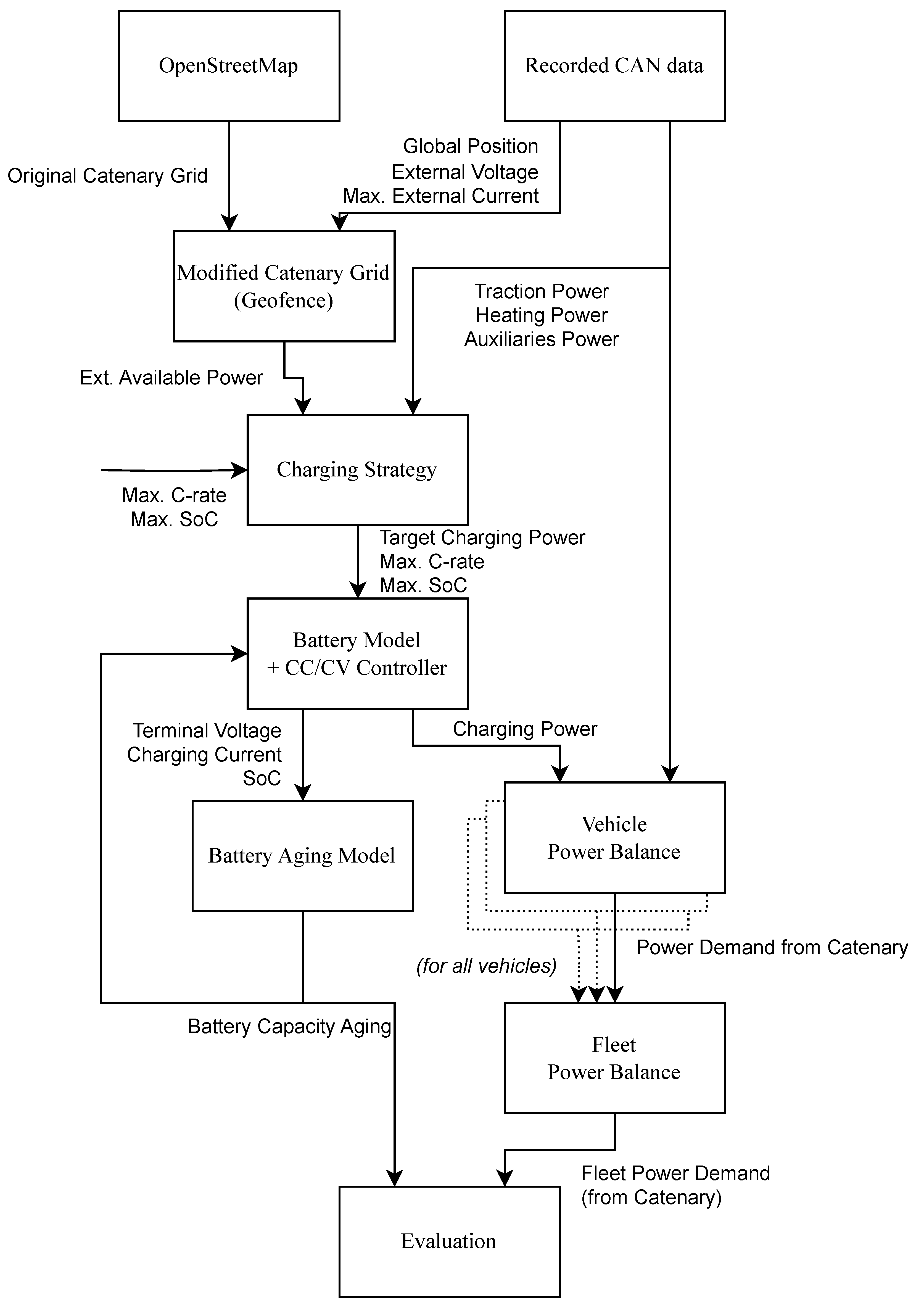
Figure 2.
Power demand of a sample trip during one day
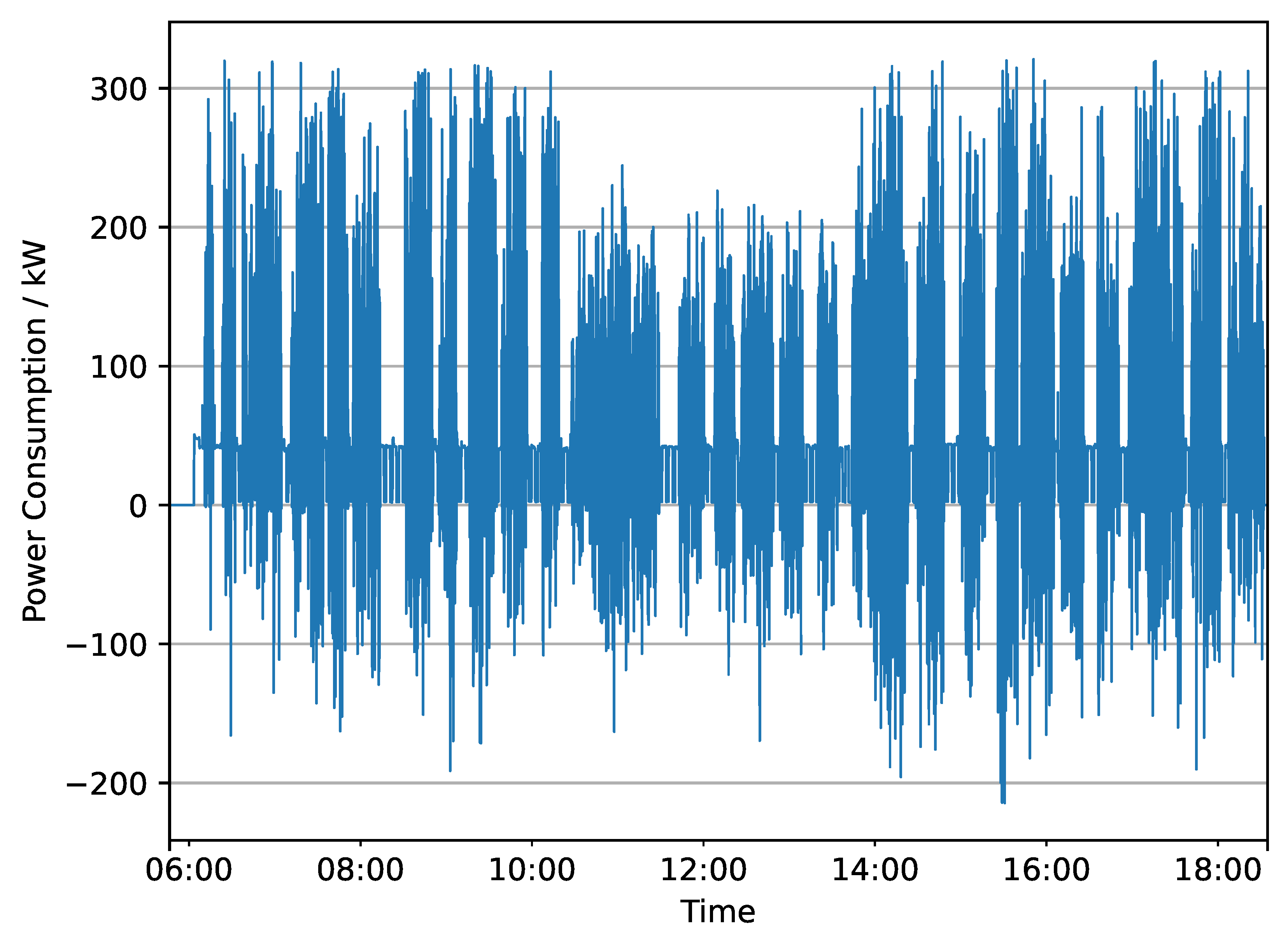
Figure 3.
Electric battery model with SoC-dependent open circuit voltage , internal resistor , terminal voltage , and charging current
Figure 3.
Electric battery model with SoC-dependent open circuit voltage , internal resistor , terminal voltage , and charging current
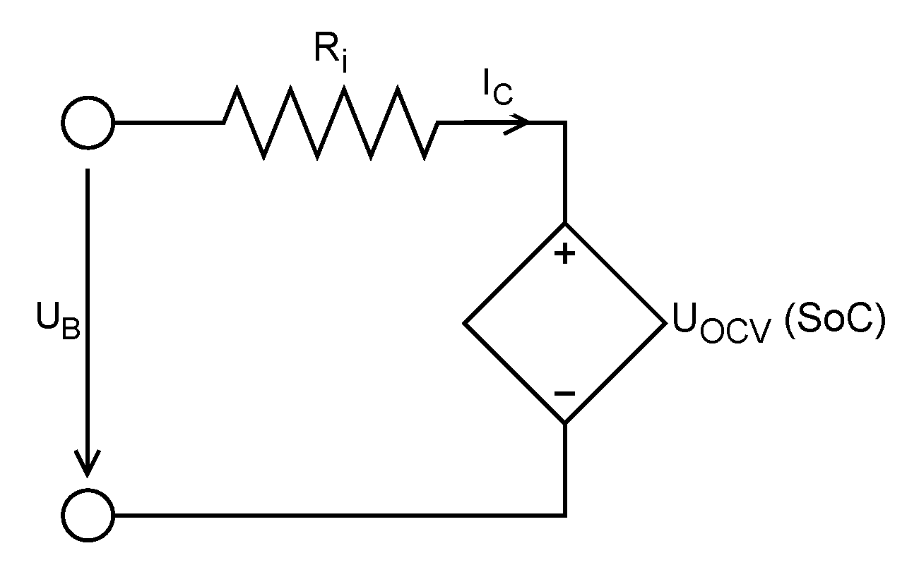
Figure 4.
Structure of Battery Aging Model
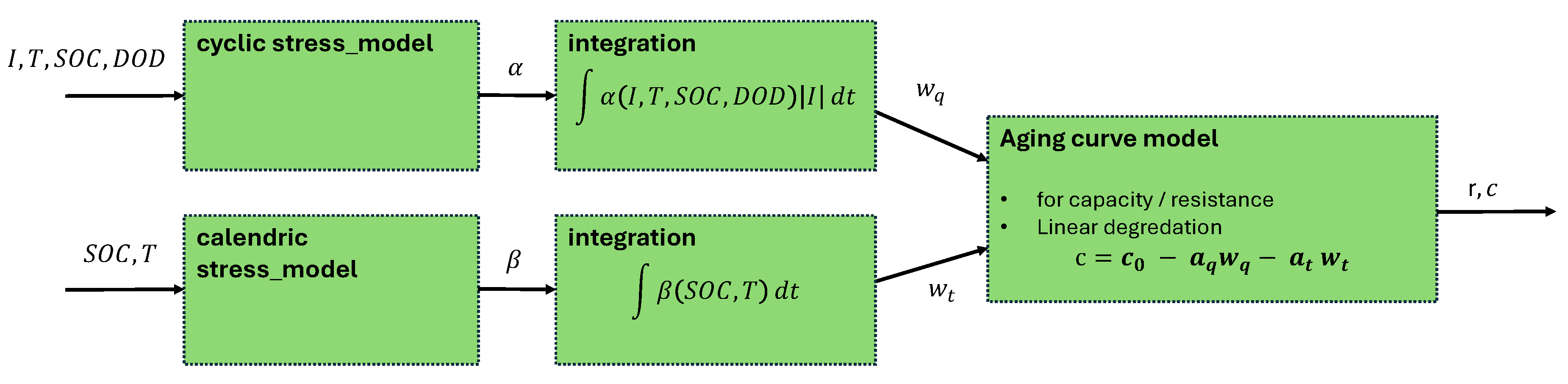
Figure 5.
SoC for the cycle denoted in Figure 2 with different charging rates and a fixed target SoC of 95%
Figure 5.
SoC for the cycle denoted in Figure 2 with different charging rates and a fixed target SoC of 95%
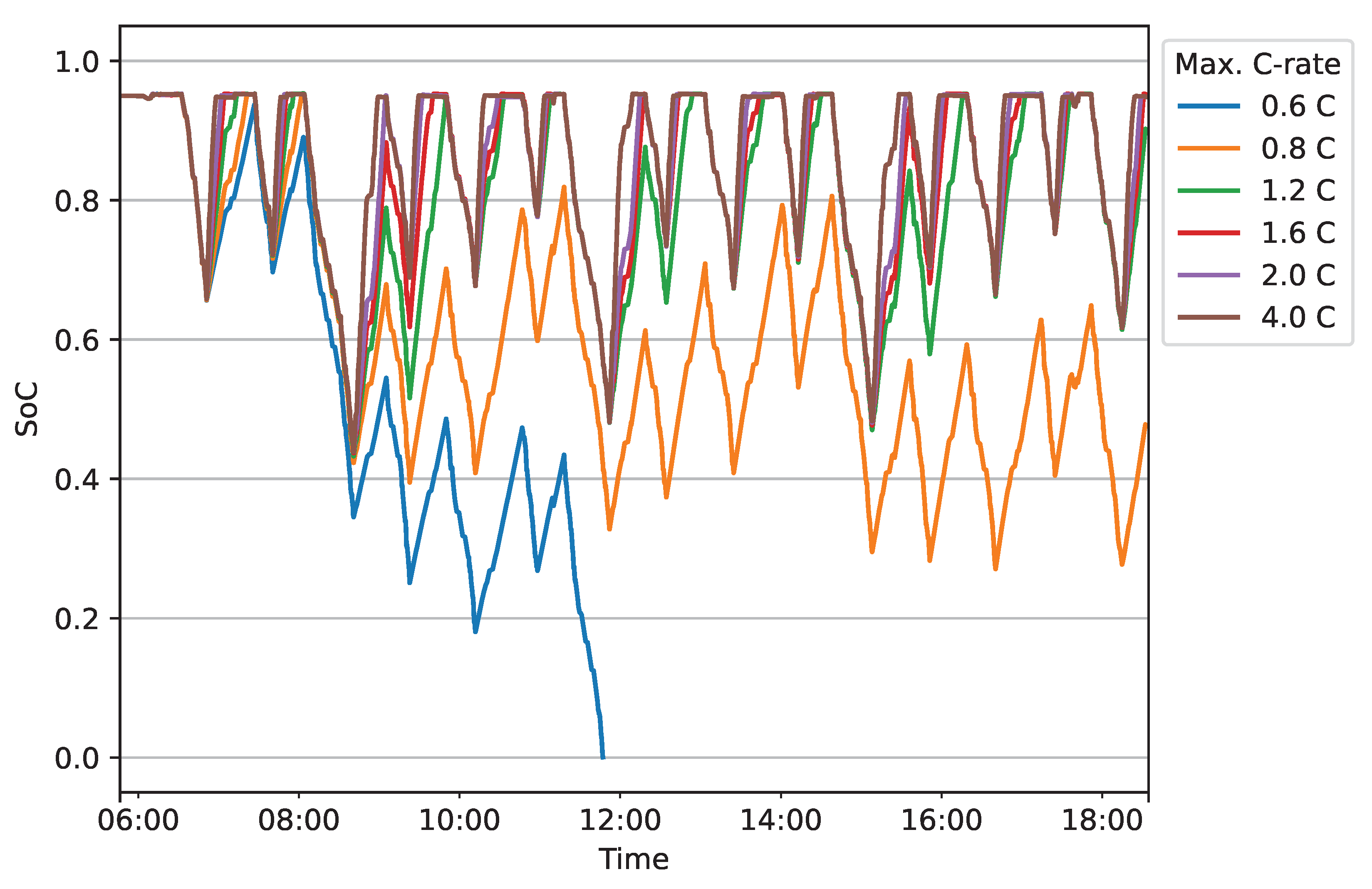
Figure 6.
SoC for the cycle denoted in Figure 2 with different target SoC and a fixed charging rate of 2 C
Figure 6.
SoC for the cycle denoted in Figure 2 with different target SoC and a fixed charging rate of 2 C
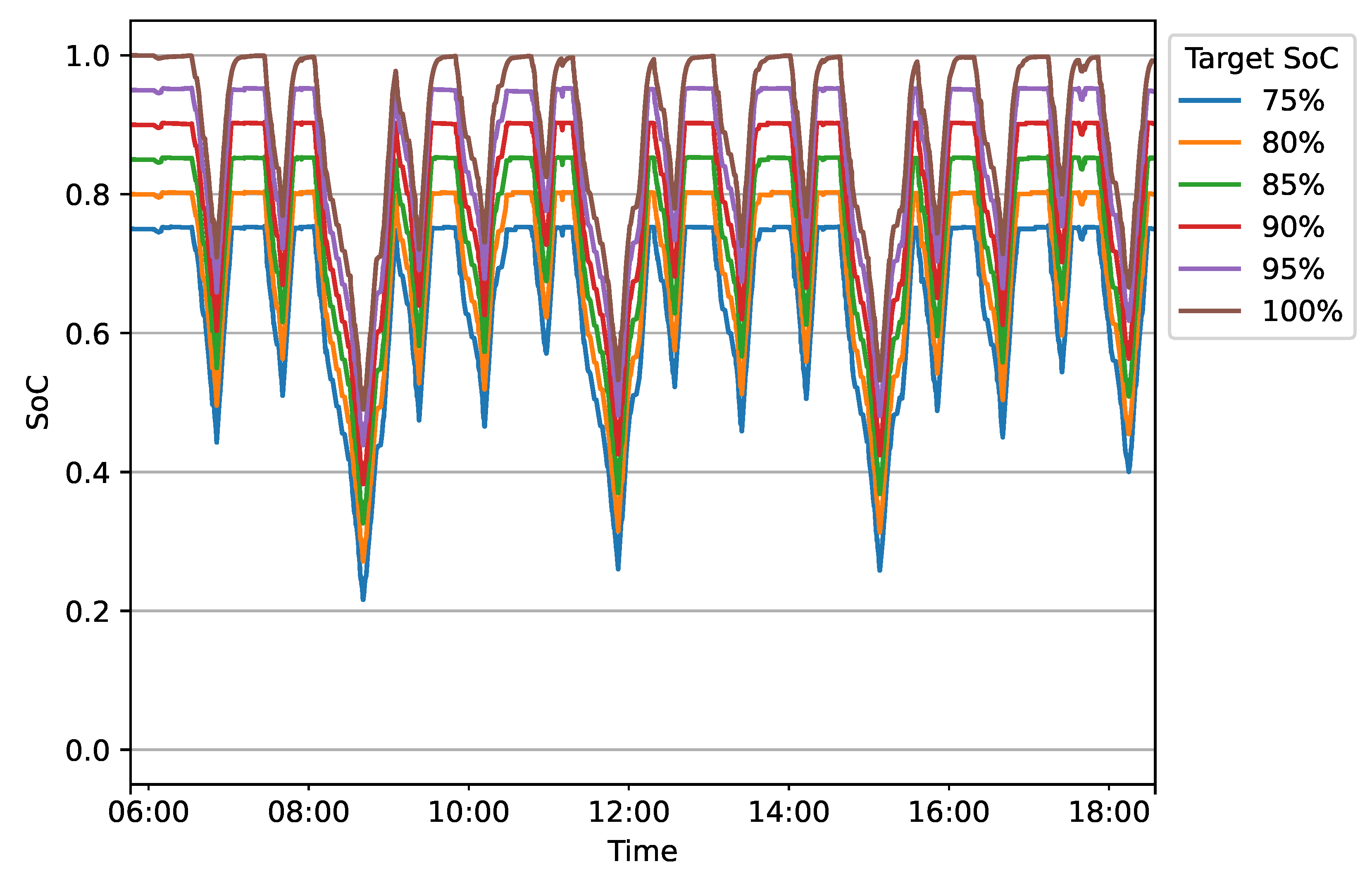
Figure 7.
Maximum, mean, and minimum fleet power draw at catenary per 15-minute interval
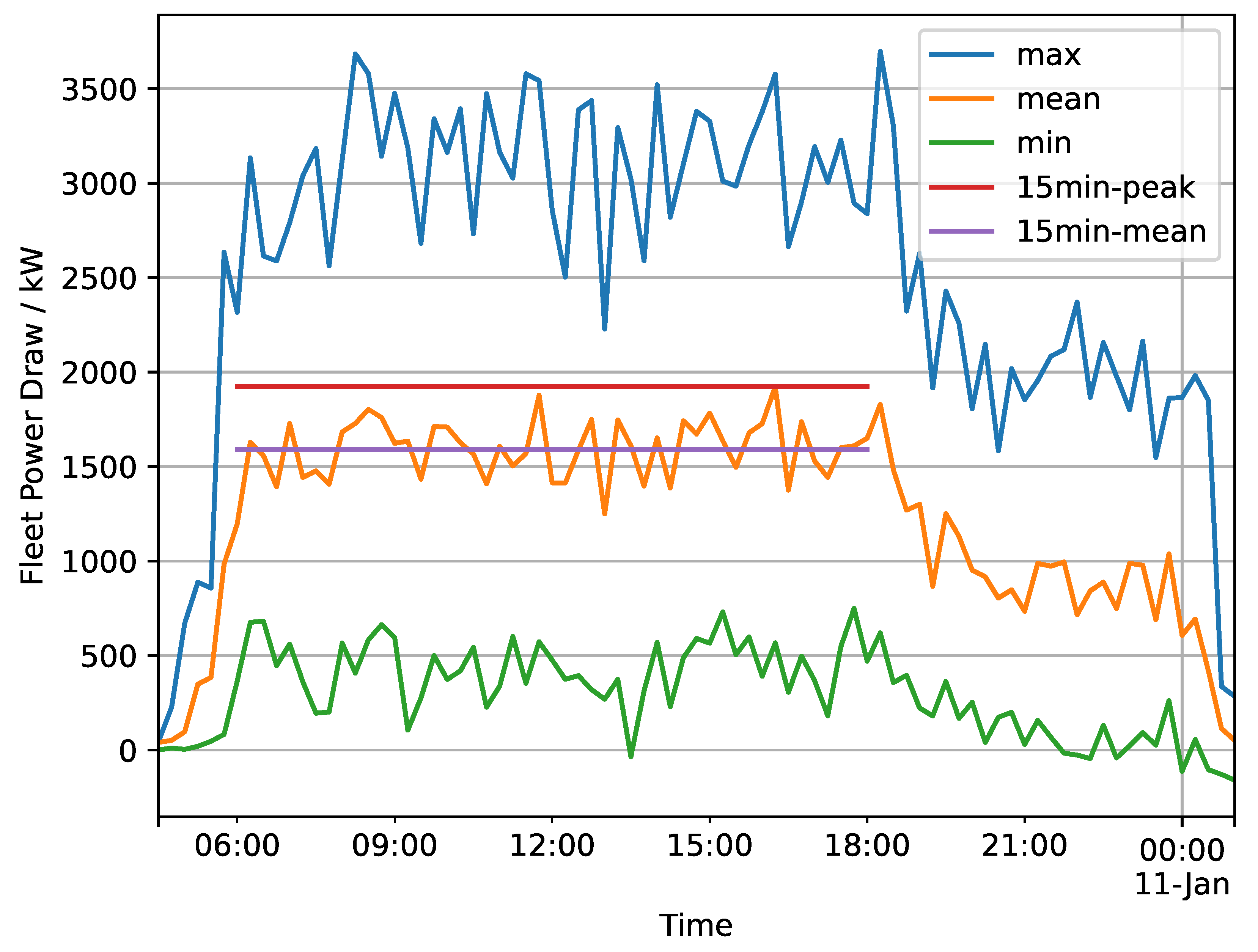

Table 1.
Recorded CAN bus data streams
| Signal | Precision | Time Interval |
|---|---|---|
| Longitude & latitude | ~0.002 ′ | 1.0 s |
| Traction power | 0.1 kW | 100 ms |
| Heating power | 0.3 kW | 100 ms |
| High-voltage auxiliary systems power | 0.1 kW | 100 ms |
| Low-voltage auxiliary systems power | 0.1 kW | 100 ms |
| Catenary voltage | 1 V | 100 ms |
| Max. catenary current | 1 A | 100 ms |
| Service trip line number | - | 1.0 s |
Table 2.
Key parameters of the investigated aging test campaign
| Batteries 2020 [31] | |
|---|---|
| Cell chemistry | Lithium Nickel Manganese Cobalt Oxides (NMC) |
| Cell capacity | 20 Ah |
| Calendric experiments | 10 |
| Cyclic experiments | 146 |
| Temperature range | 25 °C – 45 °C |
| SoC range | 0% – 100% |
| DoD range | 20% – 100% |
| C-rates | -2 C / 2 C |
Table 3.
Battery Parameters
| Cell | Pack | |
|---|---|---|
| Cell Type | NMC | |
| Pack configuration | 179 serial, 2 parallel | |
| OCV | 3.0 V – 4.2 V | 537.0 V – 751.8 V |
| Capacity | 40.6 Ah | 81.2 Ah |
| Internal resistance | 1.5 m | 134.3 m |
| Energy capacity | 151 Wh | 54.1 kWh |
Table 4.
Energy and aging metrics of the traction battery after one-day trip with different charging rates, compared to charging with 2.0 C (Brake resistor energy only considering autonomous sections)
Table 4.
Energy and aging metrics of the traction battery after one-day trip with different charging rates, compared to charging with 2.0 C (Brake resistor energy only considering autonomous sections)
| Relative Energy Consumption | Relative Brake Resistor Energy | Mean SoC | DoD | Relative Cyclic Aging | Relative Calendric Aging | Relative Capacity Aging | |
|---|---|---|---|---|---|---|---|
| Max. C-rate | |||||||
| 0.6 C | n/a | n/a | n/a | n/a | n/a | n/a | n/a |
| 0.8 C | 0.965 | 12.784 | 60.1% | 68.2% | 0.484 | 0.371 | 0.469 |
| 1.2 C | 0.996 | 5.719 | 80.4% | 52.1% | 0.713 | 0.853 | 0.732 |
| 1.6 C | 1.000 | 2.408 | 83.1% | 51.6% | 0.871 | 0.954 | 0.882 |
| 2.0 C | 1.000 | 1.000 | 84.4% | 51.4% | 1.000 | 1.000 | 1.000 |
| 4.0 C | 1.007 | 0.333 | 86.2% | 51.4% | 1.013 | 1.068 | 1.020 |
Table 5.
Energy and aging metrics of the traction battery after one-day trip with different target SoC, compared to charging until 95% (Brake resistor energy only considering autonomous sections)
Table 5.
Energy and aging metrics of the traction battery after one-day trip with different target SoC, compared to charging until 95% (Brake resistor energy only considering autonomous sections)
| Relative Energy Consumption | Relative Brake Resistor Energy | Mean SoC | DoD | Relative Cyclic Aging | Relative Calendric Aging | Relative Capacity Aging | |
|---|---|---|---|---|---|---|---|
| Target SoC | |||||||
| 75.0% | 1.003 | 0.911 | 63.6% | 53.9% | 0.924 | 0.359 | 0.849 |
| 80.0% | 1.002 | 0.859 | 68.8% | 53.4% | 0.955 | 0.484 | 0.892 |
| 85.0% | 1.002 | 0.810 | 74.0% | 52.8% | 0.988 | 0.639 | 0.941 |
| 90.0% | 1.001 | 0.758 | 79.2% | 52.2% | 1.008 | 0.812 | 0.982 |
| 95.0% | 1.000 | 1.000 | 84.4% | 51.4% | 1.000 | 1.000 | 1.000 |
| 100.0% | 1.000 | 3.462 | 88.9% | 51.0% | 0.941 | 1.173 | 0.972 |
Disclaimer/Publisher’s Note: The statements, opinions and data contained in all publications are solely those of the individual author(s) and contributor(s) and not of MDPI and/or the editor(s). MDPI and/or the editor(s) disclaim responsibility for any injury to people or property resulting from any ideas, methods, instructions or products referred to in the content. |
© 2025 by the authors. Licensee MDPI, Basel, Switzerland. This article is an open access article distributed under the terms and conditions of the Creative Commons Attribution (CC BY) license (http://creativecommons.org/licenses/by/4.0/).
Copyright: This open access article is published under a Creative Commons CC BY 4.0 license, which permit the free download, distribution, and reuse, provided that the author and preprint are cited in any reuse.


