Submitted:
12 June 2025
Posted:
13 June 2025
You are already at the latest version
Abstract
Electric buses are key in the strategy towards a greenhouse gas neutral fleet. However, their restrictions in terms of range and refueling, as well as their increased price point present new challenges for public transport companies. The article presents an energy consumption analysis with respect to ambient temperatures and average vehicle speed based exclusively on real-world data which can be used for bus disposition planning. Additionally, the State of Charge (SOC) window during operation and vehicle idle time as well as the charging power was analyzed in this case study to formulate recommendations towards a more battery-friendly treatment. Finally, the reduction of CO2 emissions compared to Diesel buses is estimated.
Keywords:
electric bus
; energy consumption
; operating strategy
; vehicle monitoring
; case study
1. Introduction
Among the 35,579 buses sold in the European Union (EU) throughout the year 2024, 18.5% of them were electrically chargeable vehicles [1]. Although diesel powered vehicles still make up the majority of sold buses (63. 1%), fully electric buses are no longer a niche market, especially with EU climate goals set to reduce greenhouse gas emissions by at least 55% by 2030 compared to 1990 levels [2].
However, with the often two to three times higher initial vehicle cost compared to internal combustion engine (ICE) buses, infrastructure investments for charging stations, and operation restrictions regarding vehicle range and downtime for charging, it is economically challenging to justify the transition to a fully electric bus fleet. Economic feasibility is usually evaluated by a total cost of ownership (TCO) study, which covers the individual demands and constraints of public transport companies [3,4,5,6].
By long-term monitoring of electric bus fleets, two main contributions to the TCO can be analyzed in detail: the specific energy consumption (SEC), in kWh/km, directly translating to energy cost for bus operation and the lifetime of the vehicle by evaluating the operating strategy and storage conditions in the context of minimizing battery degradation. The first contribution also contains key information on the disposition of vehicles for different bus circulations, as certain routes may not be possible under low-temperature conditions without an adjusted charging strategy. The latter is of importance to enhance battery lifetime, possibly for years, resulting in a lower overall TCO.
It is beyond the scope of this paper to address the details of electrochemical processes responsible for battery degradation, which are extensively studied in literature [7,8,9,10,11]. On a more general level, it is common to differentiate into calendric and cyclic aging when discussing battery degradation [9,10].
Calendric aging is exponentially increasing with cell temperature and voltage [12]. It is therefore recommended to store a battery at relatively low cell voltage and therefore low SOC (e.g. 30 %). Depending on the specific cell chemistry, additional degradation processes may modify this general behaviour e.g. accelerated aging in a certain SOC range [13,14,15]. Storing an NMC battery at around 30 % SOC can reduce the effects of calendric aging by a factor of two compared to storing at near 100 % SOC [16,17].
When discussion cyclic aging, the SOC operating window and the charge/discharge rate are of importance. Operating a battery with low DoD but high SOC level, close to 80 % - 100 %, may results in about 40 % higher capacity degradation compared to e.g. 40 % - 60 % [18]. For battery operation, a low DoD centered at around 50 % SOC or lower is ideal with details varying by cell type [18,19,20]. The charge and discharge rate also influences cyclic battery aging as charging at high currents and suboptimal battery temperatures may result in faster degradation [21,22,23].
Based on the results of battery degradation studies, general battery operating rules can be formulated positively impacting battery degradation, i.e., the reduction of battery capacity and (maximum) power output:
- Operate at low Depth of Discharge (DoD) cycles centered at about 50% SOC or lower with frequent charging
- Operate at near room temperature and store at low temperature
- Keep the battery at low SOC level when storing for longer periods of time (e.g. 30%)
- Avoid high SOC states (typically, degradation is highest at 100% SOC due to higher cell voltage)
- Charge at low power
Note that these rules are general best practices, and the ideal battery operation may be adjusted based on the exact composition. Also, these rules are formulated solely from the perspective of battery-friendly operation. Depending on the use case, it may not be economically feasible to (strictly) follow these rules as they reduce flexibility and increase downtime for charging.
To address these rules of battery-friendly vehicle operation, a fully electric bus fleet was monitored for about 2.5 years. The SEC for different operating conditions is evaluated, the SOC level during operating and idle time as well as the charging power is analyzed and recommendations are given. Additionally, the reduction of CO2 emissions compared to Diesel buses is estimated in this study.
2. Methods
2.1. Overview over Bus Fleet and Signal Set
A mixed fleet of solo and articulated fully battery-electric buses has been monitored starting mid-2022 (the exact starting date varies by bus) until February 28th, 2025. The total distance and number of operating days, as well as information about the battery, is given in Table 1.
Relevant signals from the OEM cloud service were long-time stored and evaluated using the Cloud2Cloud capabilities of the IVImon platform [24]. Relevant signals and their time resolutions are listed in Table 2.
Due to data gaps and irregularities in the temperature signal at an air vent, that could in principle be used to monitor the ambient temperature, hourly temperature values from open-meteo were taken for the evaluation [25].
2.2. Energy consumption analysis
Long-term monitoring allows for analyzing the energy consumption at different operational conditions and using this data for future disposition planning. The benefit of this approach is the data-driven nature without the need for extensive modeling as studied in literature [26,27]. There are several influencing factors regarding the energy consumption of an electric vehicle for a specific trip. Figure 1 presents a scheme of the most important indirect and direct factors considered in this paper impacting the SEC.
The speed profile is of great importance as many acceleration and deceleration processes during a trip, like in stop-and-go traffic, result in higher energy consumption. It is mainly influenced by the bus driver and regulatory factors like bus lanes and traffic lights. Especially at higher speeds, wind resistance leads to a higher SEC as well due to the quadratic influence of the vehicle speed to drag forces. The speed signal is also used for trip detection in the following way: A trip starts as soon as the speed signal is above zero and ends when the signal reaches zero and the time at rest is longer than four minutes. This prevents stop-and-go traffic and breaks at bus stops from ending the trip time period. Only trips that are longer than ten minutes are evaluated for the energy consumption analysis to prevent short maneuvers and test drives from influencing the results. For each detected trip, the average speed is calculated by dividing the total distance by the trip duration. In the context of urban buses, a lower average speed mostly indicates longer rest time at stations, traffic lights and more stop-and-go traffic in general.
An example dataset for an operational day of a bus is shown in Figure 2. Panel (a) shows the vehicle speed signal for one day of operation. In total, 11 individual trips are identified from that signal, the beginning and end of such trips are marked with a green and red vertical line, respectively.
While the ambient temperature plays a big role in energy consumption due to higher secondary consumers like heating, as well as higher power draw of the battery thermal management, wind conditions are considered neglectable for urban bus speed profiles within this paper.
Figure 2 (b) – (g) shows important quantities of one detected trip indicated by the lines connecting subplots (a) and (b). The battery power is shown in panel (e), where negative values indicate power drawn from the battery and positive values show energy recuperation from braking and the beginning of a charging process at around 15:47. The following quantities were evaluated for each trip: The distance value can be directly taken from the vehicle odometer signal by subtracting the values at the end and start of the trip. Dividing the distance by the trip duration directly yields the average speed of the trip. The energy is calculated from the mean value of the battery power signal, available with a time precision of 100 ms, multiplied by the trip duration. The ambient temperature is taken from the hourly open-meteo dataset by finding the closest timestamp to the trip after half of the trip duration. The results for the 11 trips identified in Figure 2 (a) are listed in Table 3.
The elevation profile influences the trip energy consumption heavily. When looking at the values given in Table 3, trips 2 to 10 all have nearly identical distances. However, subsequent trips have opposite elevation differences due to the same route being driven back and forth resulting in trips 2, 4, 6, 8 and 10 having up to 85 % higher SEC compared to the trips 3, 5, 7 and 9. To mostly eliminate the influence of the elevation profile of individual trips, as well as reduce the impact of outliers, a daily grouping of the trips is performed.
For the daily grouping, the distance and energy values of all trips during an operating day and of an individual bus are summed up. New energy consumption and average speed values are calculated from the summed-up distance, energy and trip duration values. To calculate daily averaged temperatures and vehicle weights, and account for the possibility of trips with largely different distances, the individual values are weighted by the trip distances:
Here, x is either the ambient temperature T or the vehicle weight m, is the daily average value, is the average value of trip i, is the distance of trip i and n is the total number of trips detected during the day of operation. The daily grouping of the individual trip values given in Table 3 results in the values given in Table 4.
The procedure was done for all operating days for each bus without discrepancies in the dataset, such as nonphysically low or large vehicle weight, with more than 50 km daily distance driven, resulting in 1,413 data points for the solo buses and 11,564 data points for articulated buses.
2.3. Usage Analysis on SOC Levels and Charging Power
In this study, the driven kilometers of electric buses within specific ranges of battery SOC are analyzed by dividing the SOC into 20 intervals ranging from 0 % to 100 % in increments of 5 %. The total kilometers driven within each SOC bin are aggregated for each day and vehicle, providing an overview of the relationship between battery state and distance traveled.
In order to evaluate the distribution of SOC during idle time of electric buses, a series of data processing functions is employed. Therefore, the SOC, vehicle speed and current flow signals as well as the odometer signal are used. The odometer signal is used to detect data gaps where the vehicle was operated. Such data gaps with an odometer signal discrepancy were discarded and therefore not counted towards vehicle idle time. Then, the data was resampled to a 1-minute frequency using interpolation methods to fill in missing values. Again, the SOC is divided into 20 intervals and for each interval, the occurrences where the vehicles is stationary (speed equal to 0) and the battery current is below 1 A is counted, resulting in a dataset containing the amount of time (in minutes, later converted into days) each bus spent idle at varying SOC levels.
To assess the charged energy (in kWh) within different ranges of charging power (in kW), the battery power signal was used. Battery charging sections were identified by finding sections were the battery power was positive for longer than 1 minute. The energy charged during each charging period was calculated using the trapezoidal integration method. The charging power was divided into intervals ranging from 0 to 300 kW in 10 kW increments and the total energy charged for each interval is aggregated.
3. Results
3.1. Analysis of the Energy Consumption per Kilometer
Based on the daily grouped dataset described in Section 2.2, the SEC was analyzed with respect to ambient temperature and average speed, the results of which are presented in Figure 3, panels (a) and (b) for the solo and articulated buses, respectively. The data points are grouped into bins of speed and temperature ranges. The speed range is given in the legend of Figure 3, the temperature range is ±1°C around the plotted data point. The points show the mean values of the energy consumption in kWh/km, with the shaded area of each curve ranging from the 10th and 90th percentile. Panels (c) and (d) show the 90th percentiles in separate plots as these values should be used for bus disposition planning.
In the ambient temperature range between 16°C and 20°C, the energy consumption is lowest for both types of buses and all average speed ranges. At temperatures above 22°C, cabin climatization and battery thermal management (cooling) increase the SEC e.g. by 13 % when comparing 18°C with 28°C ambient temperature at the (18,20) km/h speed range for articulated buses. At low temperature, the SEC increases until reaching a plateau at about 4°C ambient temperature. This is due to an additional oil heater supporting cabin climatization and thus reducing overall energy consumption. Interestingly, the 90th percentiles for the articulated buses in panel (d) keep increasing until the lowest ambient temperature value in the dataset, with an exception at -4°C and (18,20) km/h due to only 16 daily grouped data points in that temperature and speed range. This may indicate that the additional oil heater is not always operating.
The deviations of the 10th and 90th percentile compared to the mean values are typically around 8 % to 10 %. There are several influencing factors on the SEC besides average speed and ambient temperature. One is the total vehicle weight, i.e., the difference between a (nearly) empty bus and a fully occupied one. However, when analyzing the daily distance-weighted average vehicle weight, the 10th and 90th percentile only differ by about 2% from the mean values. Since vehicle weight has a linear influence on the SEC, it should in turn result in deviations of about 2% [28]. The influence of the driver is probably the biggest factor as, at least for battery-electric passenger cars, an anticipatory driving style can reduce the energy consumption by up to 16% compared to aggressive driving and 7.1 % compared to moderate driving behaviour [29]. Higher average speed results in lower overall energy consumption which is attributed to less stop-and-go traffic due to traffic lights or congestions and shorter stopping times at stations. Thus, bus acceleration in cities by prioritization at traffic lights and setting up separate bus lanes is also a cost saving factor. The difference between the (18,20) km/h and the (20,22) km/h average speed intervals is about 0.05 kWh/km.
3.2. Operational State of Charge (SOC) Analysis
To address cyclic aging of the batteries in the electric bus fleet, the accumulated driven kilometers in each SOC range are presented in Figure 4. Panels (a), (b) and (c) show the results for solo buses in the entire time frame of the monitoring, in summer and in winter, respectively. Independently of the season, the bin with the highest driven distance is the one with the SOC level between 95 % and 100 %. Out of the total driven distance of 375,141 km, only 6,617 km (or about 1.8 %) were covered at SOC levels below 50 %. In winter, the distance covered at SOC level below 50 % was only 1.5 %, compared to 3.0 % in summer. This may be due to precautions in winter. As already mentioned in rule 1 of the general battery-friendly operating rules (see Introduction), low DoD centered at 50% or lower SOC are ideal for battery operation.
Figure 4, panels (d), (e) and (f) present the same evaluation for the articulated buses. In terms of battery lifetime rules (see Introduction), the articulated buses are operated more battery-friendly than the solo buses with a 5 % lower average SOC over the full monitoring period. The 95 % to 100 % SOC bin is no longer the one with the highest driven distance. Instead, most kilometers are driven between 75 % and 95 % with a noticeable SOC level drop in winter compared to summer. During a regular operating day including opportunity charging, the battery is typically never charged up to 100 % again. The total driven distance with an SOC level below 50 % equal to 3.5 % (1.7 % in summer, 6.3 % in winter).
The most important arguments against lowering the SOC operating levels are usually added flexibility and reduced risk of running out of battery charge in case of a malfunction of the opportunity chargers. From the collected data over a period of about 2.5 years, the number of days with an SOC below 20% can be identified. At 21 days per bus per year a SOC below 20 % was reached and at 10 days the SOC dropped below 10 %. This illustrates that lowering the SOC window is feasible, especially since it is purely the result of a usage analysis without a set goal to stay above those SOC values. Also, the charging strategy can be adjusted in case of e.g. opportunity charging station failures.
3.3. Rest Period at High SOC Values
As stated in the introduction, high SOC states during rest periods has a negative impact on calendric aging of the battery. Figure 5 presents the vehicle idle time (defined by the vehicle speed equal to zero and near zero battery power and, thus, no stop due to charging) in each SOC range for (a) solo buses and (b) articulated buses. In both cases, the vehicle rest time is highest in the SOC range between 95 % and 100 % which corresponds to a (almost) fully charged battery. About 62 % of the idle time the SOC level is above 95 % for both types of buses. This is due to the buses being connected to the charger on their return to the depot. Once the battery is fully charged, the SOC stays at that level until the next driving operation. The average idle time span per 12m (18m) vehicle and day is 11.9 (11.1) hours with 7.4 (7.4) hours at above 95 % SOC. Therefore, each bus is, on average, operated or charged for more than half a day and longer idle periods rarely happen. However, a smart fleet charging management system that delays the beginning of the charging process in such a way that the battery is fully charged right before the next vehicle use would be ideal.
3.4. Analysis of Charging Power
As stated in the introduction, in context of battery degradation, the battery should be charged at low power. The charged energy at different power intervals is analyzed and shown in Figure 6 for (a) solo buses and (b) articulated buses for the year 2024. The time range for the evaluation is restricted compared to the full monitoring period due to data gaps in the first year of operation during charging processes. In general, charging powers below 140 kW are used during depot charging, whereas higher charging power up to about 290 kW is used at opportunity chargers. Note that for the batteries listed in Table 1, a 1 C charge rate corresponds to 258 kW for the solo buses and 322.5 kW for the articulated buses.
During depot charging, the solo buses are typically charged at 18 kW corresponding to 0.07 C, whereas the articulated buses are charged at either 65 kW to 70 kW (about 0.2 C, see Table 1 for battery sizes) or at twice the power depending on single or double occupation of the depot charger. Both values can be considered relatively low power which benefits battery lifetime. During opportunity charging, the buses get charged initially with 270 to (about 1.1 C for solo buses, 0.9 C for articulated buses). In panel (a), another charging power window is present between 180 kW and 240 kW which is not present for the articulated buses in panel (b). This is due to the power reduction at high SOC levels (above ) since the solo buses are often operated in the 80 % - 100 % SOC range. Such a power reduction is less apparent for the articulated buses because of a lower SOC operating window and the larger battery capacity.
3.5. Environmental Impact
Based on the monitoring data, the reduction of CO2 equivalent greenhouse gas emissions can be estimated when compared to Diesel buses, where the emission of the German electricity mix in 2023 of 380 g/kWh is assumed [30]. The total energy consumption of the 12m buses is 374.8 MWh for a total distance of 372.6 Tkm, the 18m buses have travelled 3,029.3 Tkm with 4,766.2 MWh total energy consumption. Note that this value is calculated from the battery power during operation, thus charging losses are not yet accounted for. Assuming a charging energy efficiency of 95%, this results in the emission of approximately 2,056.4 tons of CO2 (12m: 149.9 tons, 18m: 1906.5 tons) and (indirect) emission factors of 402 g/km and 787 g/km for 12m and 18m electric buses, respectively. This can be compared to an equivalent fleet of Diesel buses, where the real-world CO2 emission factor of urban city buses are reported to be 871 g/km and 1,416 g/km (average value for half load) for 12m and 18m, respectively [31,32]. Thus, an equivalent Diesel bus fleet would have emitted about 4,614.1 tons of CO2 (12m: 324.6 tons, 18m: 4,289.5 tons) or, in other words, about 2.2 times the amount of the electric bus fleet. On top, emissions of other gases like NOx, CO and THC, which are harmful to health and environment, are prevented. With the corporate sustainability reporting directive (CSRD) of the European Union [33] obligating many companies to report their greenhouse gas emissions and present an emission reduction plan, long term data monitoring allows for precise evaluations and tracking the emission reduction goals towards a greenhouse gas neutral fleet.
4. Discussion
The article presents various findings regarding energy consumption and battery operation for fleet of 2 solo buses and 18 articulated electric buses. Instead of presenting a model approach to determining the energy consumption of electric buses, a large dataset was analyzed to determine the energy consumption with respect to ambient temperature and average speed of the buses. The advantages are the straight-forward and easily-understandable results as real-world data was used exclusively. However, such an analysis requires long periods of data monitoring. The monitored buses are exclusively comprised of urban buses. Thus, the energy consumption could only be analyzed for a small window of speed ranges.
Furthermore, the operation of the bus fleet in terms of battery SOC operating window, idle time conditions and charging power was analyzed. For a battery-friendlier operation, the SOC window of operation should be shifted to lower values by about 20 %. This is more severe for the solo buses which are often operated in the SOC range between 80 % and 100 %. Additionally, a smart depot charging system that charges the buses right before the next bus operation is recommended to reduce the vehicle idle time at high SOC levels and, thus, calendar aging.
In order to safely reduce the operational SOC window, the 90th percentile curves can be used to estimate the energy demand of bus circulations and adjust the charging strategy according to ambient temperature and average speed of a bus circulation. The monitored bus fleet does not show signs of advanced battery degradation yet, which should be taken into account in the future with an aging bus fleet by suitable aging models [34,35].
The estimation of CO2 emissions reveals that an equivalent Diesel bus fleet would have emitted about 2.2 times the CO2 of the electric buses assuming the 2023 electricity mix of Germany. Therefore, the emission of about 2560 tons of CO2 was prevented corresponding to the total yearly CO2 footprint of 452 EU citizens [36].
Author Contributions
Conceptualization, T.K., R.K. and M.U.; software, T.K. and E.B.; validation, T.K.; formal analysis, T.K.; data curation, T.K.; writing—original draft preparation, T.K.; writing—review and editing, T.K., E.B., R.K. and T.L.; visualization, T.K., T.L. and E.B.; supervision, M.U.; project administration, M.U. All authors have read and agreed to the published version of the manuscript.
Funding
This research was funded within the scope of the “FRL Validierungsförderung EFRE 2021–2027, project VALA (application number 100737672)" with resources from the European Regional Development Fund (ERDF) and the Free State of Saxony.
Data Availability Statement
The datasets presented in this article are not readily available due to confidentiality with the public transport company.
Acknowledgments
The authors gratefully acknowledge the technical support of Denis Kühne and Uwe Schneider.
Conflicts of Interest
The authors declare no conflicts of interest.
Abbreviations
The following abbreviations are used in this manuscript:
| OEM | original equipment manufacturer |
| EU | European Union |
| SOC | State of Charge |
| SEC | specific energy consumption |
| SOH | State of Health |
| DoD | Depth of Discharge |
| TCO | Total Cost of Ownership |
| CSRD | corporate sustainability reporting directive |
References
- ACEA. New commercial vehicle registrations: vans +8.3%, trucks -6.3%, buses +9.2% in 2024, 2025.
- Commission, E. Communication from the Commission to the European Parliament, the Counsil, the European Econimic and Social Committee and the Committee of the Regions. Technical Report COM/2020/562 final, Brussels, 2020.
- Grauers, A.; Borén, S.; Enerbäck, O. Total cost of ownership model and significant cost parameters for the design of electric bus systems. Energies 2020, 13, 3262. [Google Scholar] [CrossRef]
- Kim, H.; Hartmann, N. Total cost of ownership analysis of battery electric buses for public transport system in a small to midsize city 2022. Publisher: International Association for Energy Economics.
- Xiao, G.; Xiao, Y.; Shu, Y.; Ni, A.; Jiang, Z. Technical and economic analysis of battery electric buses with different charging rates. Transportation Research Part D: Transport and Environment 2024, 132, 104254. [Google Scholar] [CrossRef]
- Jefferies, D.; Göhlich, D. A comprehensive TCO evaluation method for electric bus systems based on discrete-event simulation including bus scheduling and charging infrastructure optimisation. World Electric Vehicle Journal 2020, 11, 56. [Google Scholar] [CrossRef]
- Jalkanen, K.; Karppinen, J.; Skogström, L.; Laurila, T.; Nisula, M.; Vuorilehto, K. Cycle aging of commercial NMC/graphite pouch cells at different temperatures. Applied Energy 2015, 154, 160–172. [Google Scholar] [CrossRef]
- Plattard, T.; Barnel, N.; Assaud, L.; Franger, S.; Duffault, J.M. Combining a Fatigue Model and an Incremental Capacity Analysis on a Commercial NMC/Graphite Cell under Constant Current Cycling with and without Calendar Aging. Batteries 2019, 5. [Google Scholar] [CrossRef]
- Han, X.; Lu, L.; Zheng, Y.; Feng, X.; Li, Z.; Li, J.; Ouyang, M. A review on the key issues of the lithium ion battery degradation among the whole life cycle. ETransportation 2019, 1, 100005. [Google Scholar] [CrossRef]
- Edge, J.S.; O’Kane, S.; Prosser, R.; Kirkaldy, N.D.; Patel, A.N.; Hales, A.; Ghosh, A.; Ai, W.; Chen, J.; Yang, J.; et al. Lithium ion battery degradation: what you need to know. Physical Chemistry Chemical Physics 2021, 23, 8200–8221. [Google Scholar] [CrossRef]
- Xu, B.; Oudalov, A.; Ulbig, A.; Andersson, G.; Kirschen, D.S. Modeling of lithium-ion battery degradation for cell life assessment. IEEE Transactions on Smart Grid 2016, 9, 1131–1140. [Google Scholar] [CrossRef]
- Ecker, M.; Gerschler, J.B.; Vogel, J.; Käbitz, S.; Hust, F.; Dechent, P.; Sauer, D.U. Development of a lifetime prediction model for lithium-ion batteries based on extended accelerated aging test data. Journal of Power Sources 2012, 215, 248–257. [Google Scholar] [CrossRef]
- Rumberg, B.; Schwarzkopf, K.; Epding, B.; Stradtmann, I.; Kwade, A. Understanding the different aging trends of usable capacity and mobile Li capacity in Li-ion cells. Journal of Energy Storage 2019, 22, 336–344. [Google Scholar] [CrossRef]
- Rumberg, B.; Epding, B.; Stradtmann, I.; Schleder, M.; Kwade, A. Holistic calendar aging model parametrization concept for lifetime prediction of graphite/NMC lithium-ion cells. Journal of Energy Storage 2020, 30, 101510. [Google Scholar] [CrossRef]
- Keil, P.; Schuster, S.F.; Wilhelm, J.; Travi, J.; Hauser, A.; Karl, R.C.; Jossen, A. Calendar aging of lithium-ion batteries. Journal of The Electrochemical Society 2016, 163, A1872. [Google Scholar] [CrossRef]
- Baghdadi, I.; Briat, O.; Delétage, J.Y.; Gyan, P.; Vinassa, J.M. Lithium battery aging model based on Dakin’s degradation approach. Journal of Power Sources 2016, 325, 273–285. [Google Scholar] [CrossRef]
- Torregrosa, A.J.; Broatch, A.; Olmeda, P.; Agizza, L. A semi-empirical model of the calendar ageing of lithium-ion batteries aimed at automotive and deep-space applications. Journal of Energy Storage 2024, 80, 110388. [Google Scholar] [CrossRef]
- Gao, Y.; Jiang, J.; Zhang, C.; Zhang, W.; Jiang, Y. Aging mechanisms under different state-of-charge ranges and the multi-indicators system of state-of-health for lithium-ion battery with Li (NiMnCo) O2 cathode. Journal of Power Sources 2018, 400, 641–651. [Google Scholar] [CrossRef]
- Preger, Y.; Barkholtz, H.M.; Fresquez, A.; Campbell, D.L.; Juba, B.W.; Romàn-Kustas, J.; Ferreira, S.R.; Chalamala, B. Degradation of commercial lithium-ion cells as a function of chemistry and cycling conditions. Journal of The Electrochemical Society 2020, 167, 120532. [Google Scholar] [CrossRef]
- de Hoog, J.; Timmermans, J.M.; Ioan-Stroe, D.; Swierczynski, M.; Jaguemont, J.; Goutam, S.; Omar, N.; Van Mierlo, J.; Van Den Bossche, P. Combined cycling and calendar capacity fade modeling of a Nickel-Manganese-Cobalt Oxide Cell with real-life profile validation. Applied Energy 2017, 200, 47–61. [Google Scholar] [CrossRef]
- Gao, Z.; Xie, H.; Yang, X.; Niu, W.; Li, S.; Chen, S. The Dilemma of C-Rate and Cycle Life for Lithium-Ion Batteries under Low Temperature Fast Charging. Batteries 2022, 8. [Google Scholar] [CrossRef]
- Kim, D.H.; Lee, J.; Shin, K.; Kim, K.B.; Chung, K.Y. Empirical Capacity Degradation Model for a Lithium-Ion Battery Based on Various C-Rate Charging Conditions. Journal of Electrochemical Science and Technology 2024, 15, 414–420. [Google Scholar] [CrossRef]
- Schreiber, M.; Gamra, K.A.; Bilfinger, P.; Teichert, O.; Schneider, J.; Kröger, T.; Wassiliadis, N.; Ank, M.; Rogge, M.; Schöberl, J.; et al. Understanding lithium-ion battery degradation in vehicle applications: Insights from realistic and accelerated aging tests using Volkswagen ID.3 pouch cells. Journal of Energy Storage 2025, 112, 115357. [Google Scholar] [CrossRef]
- Fraunhofer IVI. Remote Battery Diagnosis, 2025. Available online: https://www.ivi.fraunhofer.de/en/research-fields/electromobility/remote-battery-diagnosis.html.
- Zippenfenig, P. Open-Meteo.com Weather API, 2023. [CrossRef]
- Al-Ogaili, A.S.; Al-Shetwi, A.Q.; Al-Masri, H.M.; Babu, T.S.; Hoon, Y.; Alzaareer, K.; Babu, N.P. Review of the estimation methods of energy consumption for battery electric buses. Energies 2021, 14, 7578. [Google Scholar] [CrossRef]
- Abdelaty, H.; Mohamed, M. A prediction model for battery electric bus energy consumption in transit. Energies 2021, 14, 2824. [Google Scholar] [CrossRef]
- Weiss, M.; Cloos, K.C.; Helmers, E. Energy efficiency trade-offs in small to large electric vehicles. Environmental Sciences Europe 2020, 32, 1–17. [Google Scholar] [CrossRef]
- Al-Wreikat, Y.; Serrano, C.; Sodré, J.R. Driving behaviour and trip condition effects on the energy consumption of an electric vehicle under real-world driving. Applied Energy 2021, 297, 117096. [Google Scholar] [CrossRef]
- Icha, P.; Lauf, D.T. Entwicklung der spezifischen Treibhausgas-Emissionen des deutschen Strommix in den Jahren 1990 - 2023. Technical Report CLIMATE CHANGE 23/2024, Umweltbundesamt, Dessau-Roßlau, 2024. ISSN: 1862-4359.
- Özener, O.; Özkan, M. Fuel consumption and emission evaluation of a rapid bus transport system at different operating conditions. Fuel 2020, 265, 117016. [Google Scholar] [CrossRef]
- Zhang, S.; Wu, Y.; Liu, H.; Huang, R.; Yang, L.; Li, Z.; Fu, L.; Hao, J. Real-world fuel consumption and CO2 emissions of urban public buses in Beijing. Applied Energy 2014, 113, 1645–1655. [Google Scholar] [CrossRef]
- European Parliament and Council of the European Union. Directive (EU) 2022/2464 of the European Parliament and of the Council of 14 December 2022 amending Regulation (EU) No 537/2014, Directive 2004/109/EC, Directive 2006/43/EC and Directive 2013/34/EU, as regards corporate sustainability reporting. Official Journal of the European Union, 2022; L 322, 15–80. [Google Scholar]
- Lehmann, T.; Weiß, F. Lithium-Ion Battery Aging Analysis of an Electric Vehicle Fleet Using a Tailored Neural Network Structure. Applied Sciences 2023, 13, 4448. [Google Scholar] [CrossRef]
- Lehmann, T.; Berendes, E.; Kratzing, R.; Sethia, G. Learning the Ageing Behaviour of Lithium-Ion Batteries Using Electric Vehicle Fleet Analysis. Batteries 2024, 10, 432. [Google Scholar] [CrossRef]
- EDGAR (Emissions Database for Global Atmospheric Research). EDGAR Community GHG Database, 2024. Published: Version EDGAR_2024_GHG.
Figure 1.
Scheme of the most important factors influencing the SEC. The light green factors are directly addressed in the energy consumption analysis. Dark green factors are indirectly addressed by the daily grouping and blue factors are neglected so far.
Figure 1.
Scheme of the most important factors influencing the SEC. The light green factors are directly addressed in the energy consumption analysis. Dark green factors are indirectly addressed by the daily grouping and blue factors are neglected so far.
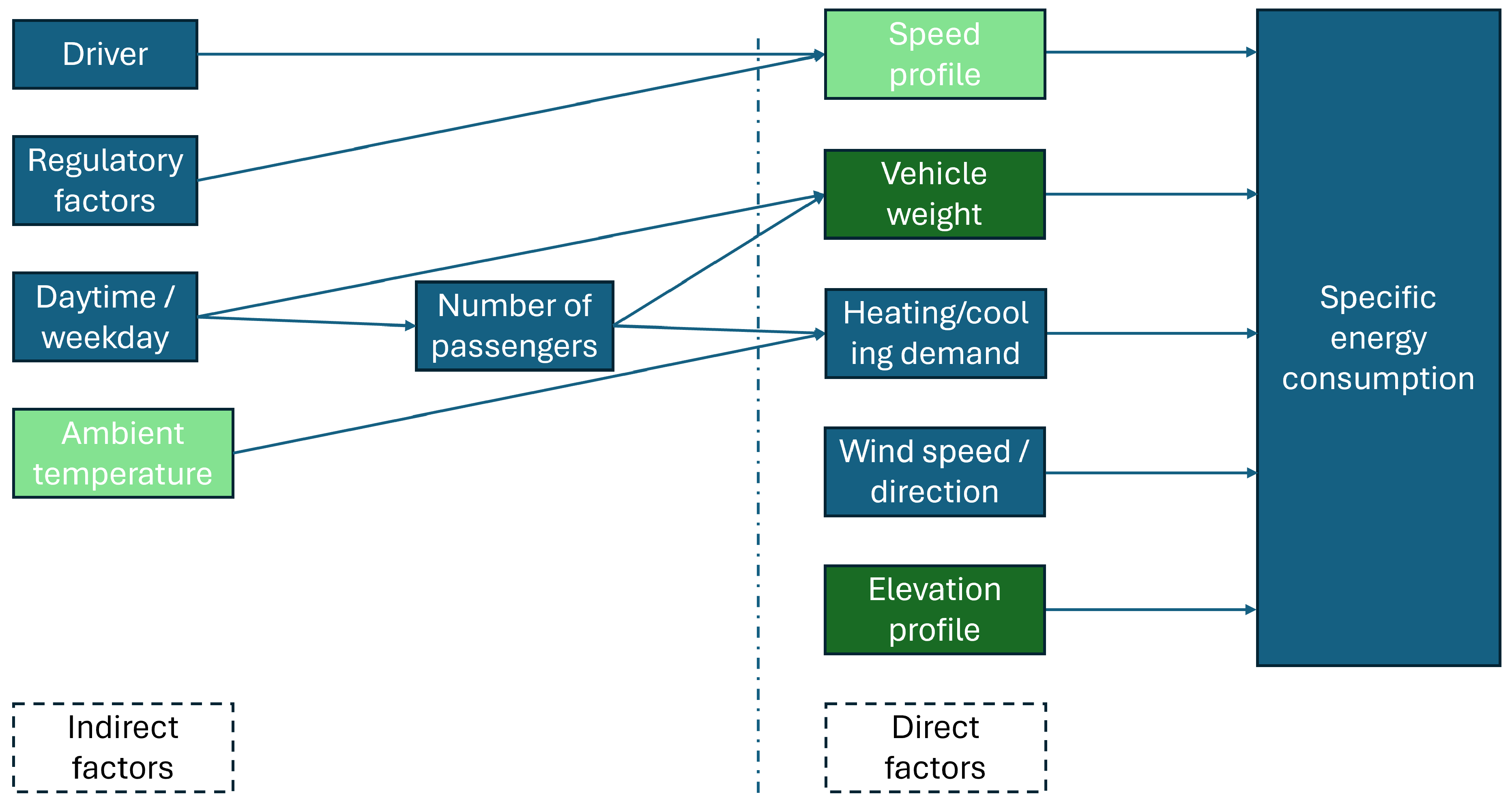
Figure 2.
Example operating day with identified trips using the vehicle speed signal. (a) Vehicle speed for the entire operation day. (b) Vehicle speed timeseries of an identified trip (see markings). (c) – (g) various signals within the time span of the example trip (see y-axis labels). Note that in (e), negative values of the battery power indicate power drawn from the battery, positive values charge the battery.
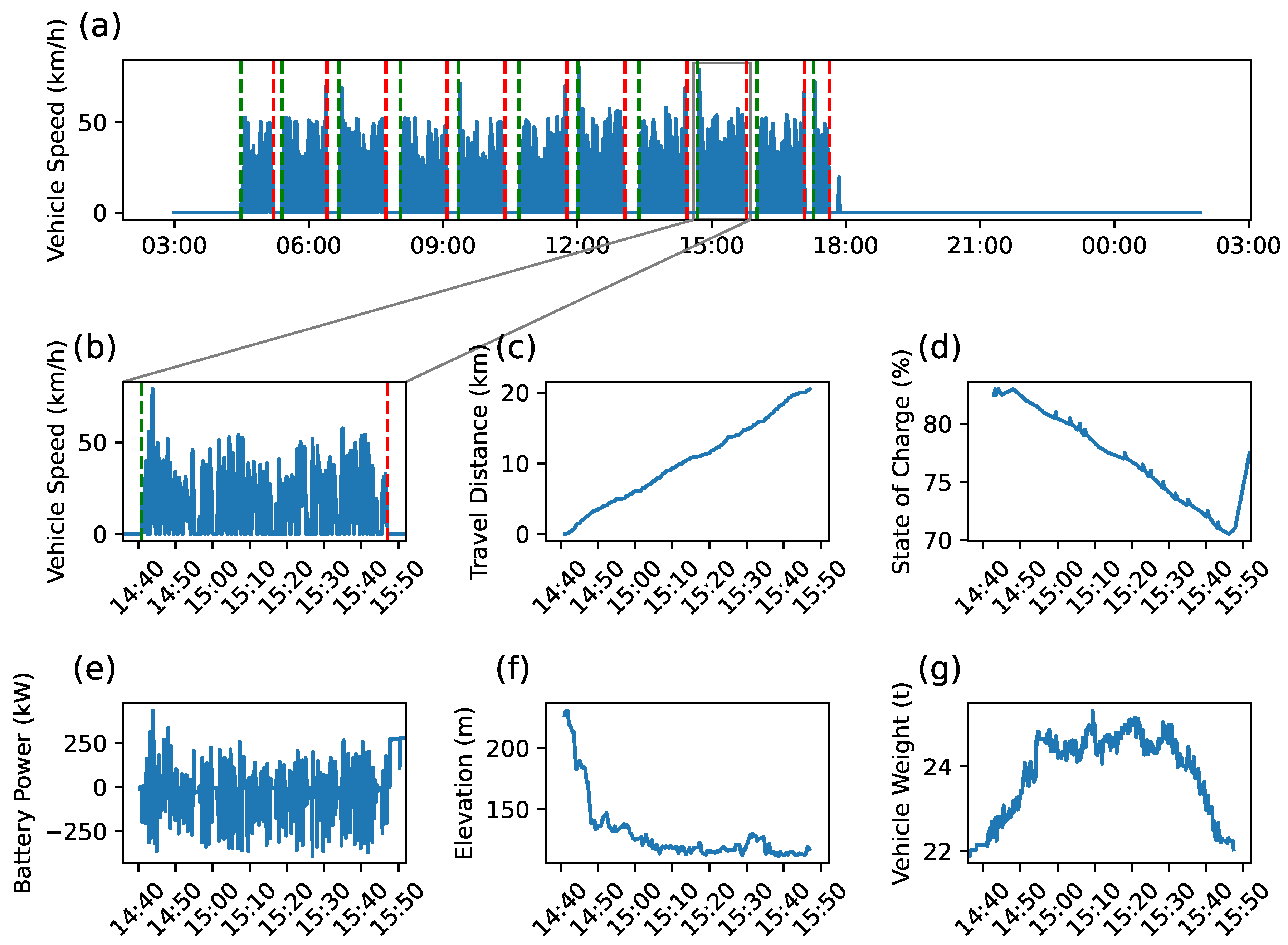
Figure 3.
Energy consumption in kWh/km vs. ambient temperature at different average speed ranges. (a) Mean energy consumption for solo buses and (b) articulated buses with the 10th and 90th percentile given by the shaded area. (c) Separate plots for the 90th percentile of the energy consumption for solo and (d) articulated buses as a useful quantity for disposition planning. Note that below 4°C an additional oil heater is used to heat the bus interior reducing overall energy consumption.
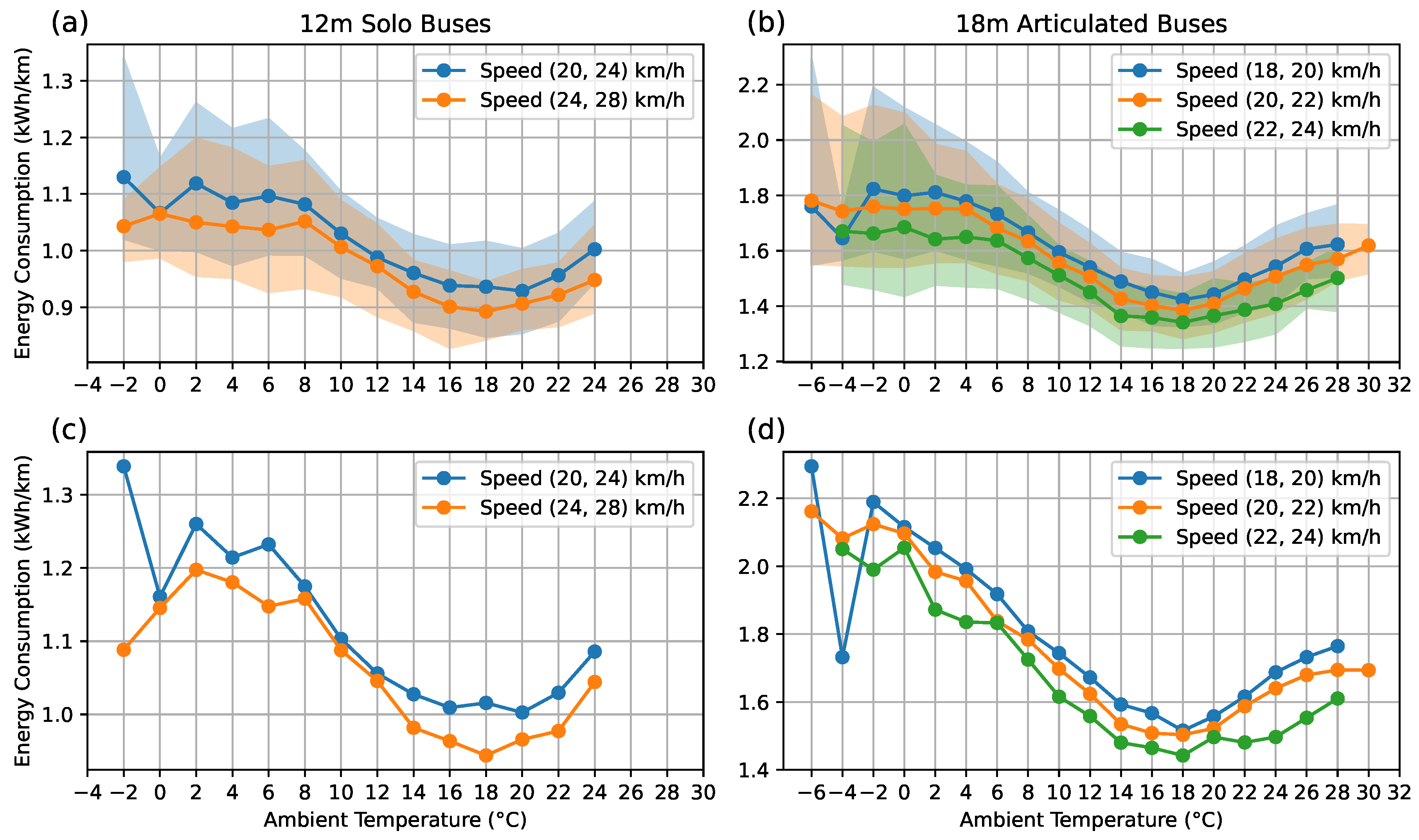
Figure 4.
Driven kilometers in the given SOC range for (a) the entire monitoring period, (b) Summer months (June, July, August) and (c) winter months (December, January, February). Due to the higher energy consumption, the average SOC is roughly 6% lower in winter than in summer. However, regarding the rules for increasing battery lifetime, the operating window should be shifted to lower SOC.
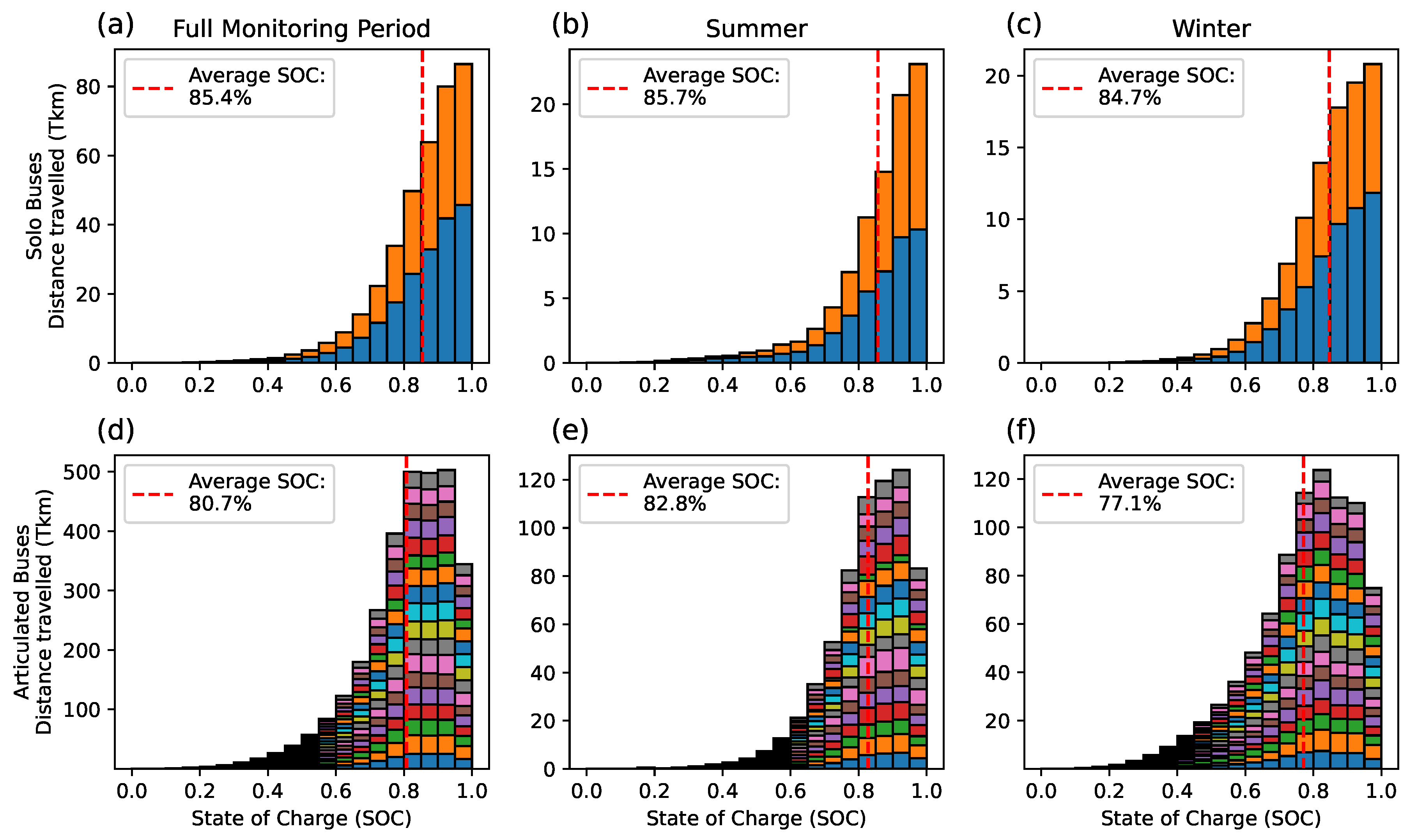
Figure 5.
Vehicle idle time (vehicle at rest and no charging process detected) at given SOC level for (a) solo buses and (b) articulated buses.
Figure 5.
Vehicle idle time (vehicle at rest and no charging process detected) at given SOC level for (a) solo buses and (b) articulated buses.
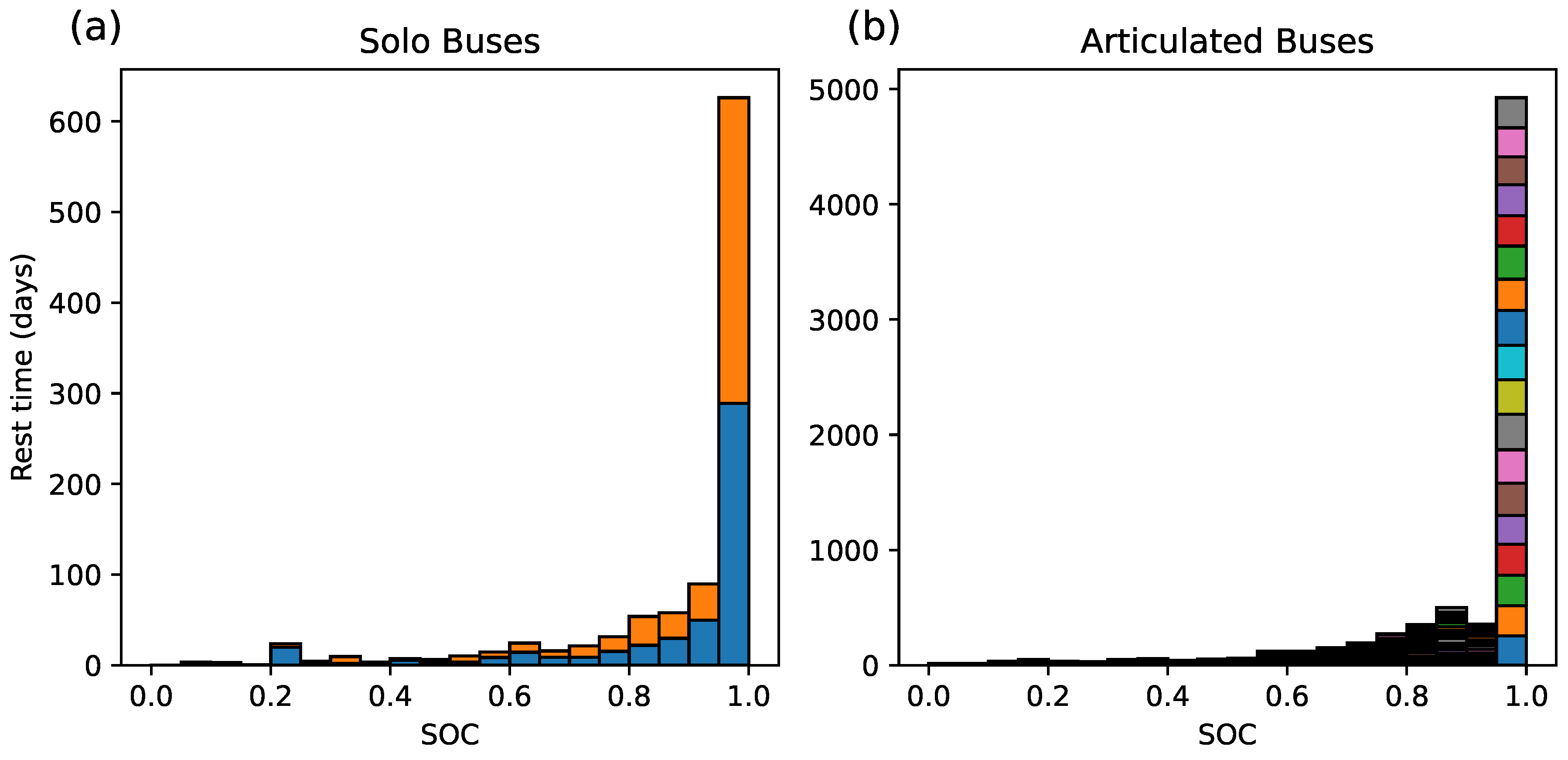
Figure 6.
Charged energy at different charging power for (a) solo buses and (b) articulated buses throughout the year 2024. Charging power below 100 kW typically indicate depot charging, whereas higher charging power is used at opportunity chargers.
Figure 6.
Charged energy at different charging power for (a) solo buses and (b) articulated buses throughout the year 2024. Charging power below 100 kW typically indicate depot charging, whereas higher charging power is used at opportunity chargers.
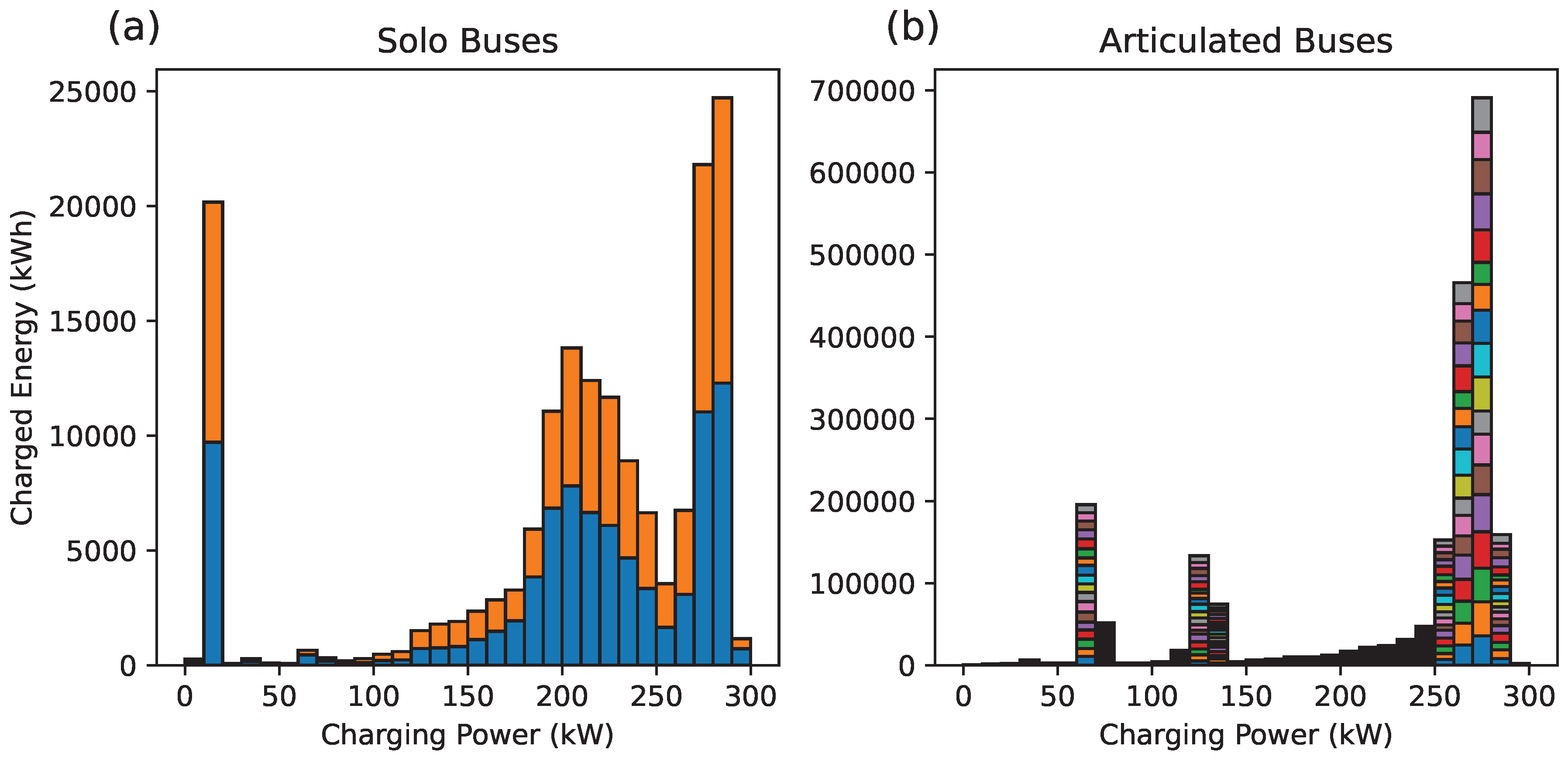

Table 1.
Overview of the monitored bus fleet. The number of operating days was identified within the energy consumption analysis (see Section 2.2) where data gaps and inconsistencies are discarded.
Table 1.
Overview of the monitored bus fleet. The number of operating days was identified within the energy consumption analysis (see Section 2.2) where data gaps and inconsistencies are discarded.
| Bus Type | Total Monitored Distance (Tkm) | Total Days in Monitoring | Total Operating Days | Battery |
|---|---|---|---|---|
| solo bus, 12m | 372.6 | 2,030 | 1,413 | 258 kWh, NMC |
| articulated bus, 18m | 3,029.3 | 16,033 | 11,564 | 322.5 kWh, NMC |
Table 2.
Vehicle signals and their time resolution used for evaluations. Temperature values are obtained from open-meteo [25].
Table 2.
Vehicle signals and their time resolution used for evaluations. Temperature values are obtained from open-meteo [25].
| Signal | Unit | Time resolution |
|---|---|---|
| Battery Power | kW | 100 ms |
| Battery Current | A | 100 ms |
| State of Charge (SOC) | % | On value-change |
| Vehicle Speed | km/h | 100 ms |
| Total mileage | km | 1 s |
| Vehicle weight | kg | 200 ms |
| GPS altitude | m | Few seconds (varying) |
| Ambient Temperature | °C | 1 h |
Table 3.
Evaluated values for the 11 individual trips for the dataset shown in Figure 2.
Table 3.
Evaluated values for the 11 individual trips for the dataset shown in Figure 2.
| Trip Nr. | Distance (km) | Energy (kWh) | Average Speed (km/h) | Ambient Temperature (°C) | Average Vehicle weight (t) | Elevation Difference (m) | SEC (kWh/km) |
|---|---|---|---|---|---|---|---|
| 1 | 15.58 | 30.86 | 21.52 | 0.8 | 22.62 | 32.0 | 1.98 |
| 2 | 20.73 | 53.75 | 20.47 | 0.8 | 24.26 | 113.0 | 2.59 |
| 3 | 20.61 | 36.68 | 19.60 | 2.4 | 23.87 | -124.3 | 1.78 |
| 4 | 20.72 | 43.52 | 20.10 | 6.8 | 24.58 | 123.9 | 2.10 |
| 5 | 20.60 | 25.56 | 20.02 | 8.3 | 24.03 | -117.6 | 1.24 |
| 6 | 20.70 | 47.40 | 19.58 | 9.8 | 24.22 | 118.3 | 2.29 |
| 7 | 20.58 | 31.84 | 19.62 | 10.3 | 23.60 | -113.8 | 1.55 |
| 8 | 20.68 | 45.79 | 19.41 | 10.1 | 23.68 | 111.0 | 2.21 |
| 9 | 20.51 | 33.02 | 18.60 | 9.9 | 24.21 | -109.1 | 1.61 |
| 10 | 20.75 | 45.64 | 19.61 | 7.4 | 23.25 | 108.1 | 2.20 |
| 11 | 8.17 | 7.58 | 23.33 | 7.4 | 22.47 | -108.2 | 0.93 |
Table 4.
Daily grouped trip values evaluated from the individual trip values given in Table 3 and shown in Figure 1.
| Distance (km) | Energy (kWh) | Average Speed (km/h) | Distance-weighted Average Temperature (°C) | Distance-weighted Average Vehicle Weight (t) | SEC (kWh/km) |
|---|---|---|---|---|---|
| 209.61 | 401.64 | 19.91 | 6.83 | 23.81 | 1.92 |
Disclaimer/Publisher’s Note: The statements, opinions and data contained in all publications are solely those of the individual author(s) and contributor(s) and not of MDPI and/or the editor(s). MDPI and/or the editor(s) disclaim responsibility for any injury to people or property resulting from any ideas, methods, instructions or products referred to in the content. |
© 2025 by the authors. Licensee MDPI, Basel, Switzerland. This article is an open access article distributed under the terms and conditions of the Creative Commons Attribution (CC BY) license (http://creativecommons.org/licenses/by/4.0/).
Copyright: This open access article is published under a Creative Commons CC BY 4.0 license, which permit the free download, distribution, and reuse, provided that the author and preprint are cited in any reuse.


