
Submitted:
10 June 2025
Posted:
12 June 2025
You are already at the latest version
Abstract
A reliable geothermal risk assessment methodology is key to any business decision. To be effective, it must be based on widely accepted principles, be easy to apply, be auditable and produce consistent results. In this paper we review the key characteristics of a geothermal project and propose a novel approach derived from risk and uncertainty definitions used in the hydrocarbon industry. Ac-cording to the proposed methodology, the probability of success is assessed by estimating three different components. The first, the geological Probability of Success (PoS), is the likelihood that the key fundamental geological elements are present. The absence of one or more of these will lead to the inevitable failure of the project. The second, the temperature threshold PoS, is defined as the probability that the fluid is above a certain reference value. Such a reference value is the one used to design the development. Such a component therefore depends on the end use of the geothermal resource. The third component is the commercial PoS and estimates the chance of a project being commercially viable using the Reverse Enthalpy Methodology (REM). Geothermal projects do not have a single parameter that represents their value. Therefore, in order to estimate it, it is necessary to make an initial assumption that can be revisited later in an iterative manner. REM works with either the capital expenditure (CAPEX) of the geothermal facility (power plant or direct thermal use) or the drilling CAPEX as the initial assumption. Varying the other parameter, it estimates the probability of having a Net Present Value (NPV) higher than zero.
Keywords:
geothermal
; exploration
; development
; geological risk
; uncertainty
; well deliverability
; economics
; investment decision
1. Introduction
This article is a revised and expanded version of a paper entitled Risk and Uncertainty assessment for geothermal projects using Reverse Enthalpy Methodology, which was presented at European Geothermal Congress 2025—EGEC 2025 Zurich, Switzerland 6-10 October 2025 [1].
The workflows for geothermal project development in well-documented historical exploitation areas are well established and effective. They involve the use of geophysical and well data to characterise the geothermal system and its development, including detailed modelling of reservoir fluid dynamics, heat flow, wells and facilities. Such analysis directly allows estimation of resource size, well and plant costs, and informed economic analysis [2,3,4,5]. In areas of newer geothermal development, this level of data is often not available to enable such analysis. Assessing the likelihood of commercial success has been the subject of much work in geothermal exploration in recent years [6,7,8]. However, few have addressed this type of project-scale assessment in areas of relatively immature exploration.
In this paper, we propose a consistent methodology to assess geological risk, uncertainty and commercial probability of success (PoS), using an approach based on hydrocarbon industry principles in which the various parameters are subjected to analysis and evaluation in several stages. We refer to such principles because they are simple, clear and have a long history of successful application in the oil and gas industry. The intention is not to blindly apply hydrocarbon practices to geothermal, but to modify them appropriately for significant differences that geothermal developments present. Identifying a systematic, repeatable, generic path to commercial success for geothermal opportunities is a key objective. The approach works in principle with all types of geothermal fields, conventional or EGS (Enhanced Geothermal System), including any use for direct heat or power generation. It is also fully compatible with the PRMS and UNECE classification systems [9,10,11,12].
2. Geological Risk, Uncertainty and Probability of Commercial Success
In this section we present the key principles of the oil and gas industry so that they can be most effectively adapted to the very different characteristics of the geothermal context.
2.1. Exploration Geological Risk
In the petroleum industry, the concept of geological risk is often defined as the probability of drilling a well and not finding flowable hydrocarbons [8,13]. This risk in a hydrocarbon context is directly related to the presence or absence of the fundamental geological elements of a hydrocarbon field. The absence of one of these fundamental elements (source rock, reservoir, etc.), or the wrong timing, is sufficient to prevent the accumulation of hydrocarbons. Geological risk is therefore represented by a binary distribution: success or failure. Note that colloquially we talk about risk, but when we evaluate a project, we calculate the Probability of Geological success (Pg). The conversion is straightforward:
Pg =100% − risk
2.2. Uncertainties and Probability Distribution Function
Uncertainty signals a lack of knowledge about extent or magnitude of a parameter. In relation to recoverable hydrocarbons, uncertainty is represented by the question: have we found a very small amount of hydrocarbons or a huge quantity? Probability Distribution Functions (PDFs) are a powerful and widely used method for describing uncertainty. They provide a complete characterization of uncertainty by assigning a probability to each possible value a parameter can take. This probabilistic representation not only defines the range of possible values but also conveys essential statistical information such as the central tendency (mean, median, mode) and the spread (variance, standard deviation), enabling a comprehensive understanding of both the expected value and the variability of the parameter. The standard deviation, variance and P10/P90 ratio of the PDF are all common and effective measures of uncertainty level. The Monte Carlo method combines multiple PDFs of different parameters with defined relationships between them to model complex uncertainties. PDFs can be described loosely by the shape they take, and the best approximating mathematical functions corresponding to that shape. In a “normal” distribution the mean, P50 and mode are the same, but in a “lognormal” curve the mean is higher than the P50 and much higher than the mode. In nature simple parameters tend to have a normal distribution [15]. More complex variables that depend on a multiplication of individual distributions—including resource volumes in the geosciences—tend to be lognormal by virtue of the central limit theorem [14,15,16]. The Cumulative Distribution Function (CDF) can be used instead as an equivalent (Figure 1). A CDF is simply a different way of presenting a given PDF. In a CDF, “P50” defines the value around which 50% of the outcomes are higher and 50% are lower. Similarly, “P10” has 10% of the values higher and 90% lower, and finally ”P90” has 90% of the values higher, and so on. Note that institutional conventions may differ with P(x) and P(100-x) definitions interchanged (e.g., P90 & P10 etc). The CDF is an effective tool because it reveals at a glance the probability of achieving a result less than or greater than a certain threshold value.
2.3. Probability of Commercial Success
In the oil and gas industry, the volume of recoverable hydrocarbons in a field is the key variable in determining the value of a project. Larger fields are proportionally more profitable. This is due to economies of scale: the cost per barrel of oil produced decreases as the size of the field increases. The resource distribution for an exploration prospect includes possible results that are too small to be commercial.
A CDF is therefore characterised by a portion that is commercial and a portion that is not. These two portions can be distinguished by calculating the Minimum Commercial Field Size (MCFS) of an exploration project (Figure 2) [14,17]. The MCFS is the volume of resources that has a Net Present Value (NPV) of zero: the “breakeven” value. All possible results greater than the MCFS are commercially viable and have an NPV greater than zero. NPV is a term which incorporates the time value of money—and associated “discount rates” which will vary with company ambitions and interest rates in different locations.
The probability of finding resources equal to, or larger than the MCFS is defined as the probability of commercial success (Pc).
2.4. Overall Probability of Success of an Exploration Oil&Gas Project
Thus, Pg (as seen in subsection 2.1) is the probability of having a discovery, while Pc is the probability that such a discovery is large enough to have an NPV equal to or greater than zero [17]. Therefore, the probability of finding a commercial amount of hydrocarbon is the combined probability of Pg and Pc:
Total PoS of an exploration project = Pg * Pc
Similar to an oil and gas exploration project, such an approach can be used to estimate the PoS of a geothermal exploration project. However, defining the right parameter to use to estimate it is not as straightforward as in the hydrocarbon industry. This issue is discussed in the following sections.
3. Framing Risk and Uncertainty of a Geothermal Project
Geothermal energy is a renewable energy source that harnesses heat from the Earth’s interior. Some geothermal exploitations utilise water or steam fluids already present within rocks (hydrothermal) and others rely on heat of drier rocks and either engineered permeability or conduction of heat into fluids of a wellbore (petrothermal). We address the hydrothermal case in this paper as the one with the most generically applicable set of risk elements, but the principles can be applied to petrothermal applications.
From a hydrothermal reservoir, hot fluids are produced to the surface through wells and used to generate electricity or provide direct heating. To apply the above principles we differentiate elements to be considered in the risk system and those parameters affecting the level of uncertainty of the geothermal project.
3.1. Key Premises and Assumptions of the Risk System
3.1.1. Key Geological Elements
The importance of key geological elements such as fluid temperature and chemistry, reservoir permeability, sealing properties, etc. in geothermal systems varies depending on the development chosen.
For a given geology, the temperature of the geothermal fluid (for a single-phase geothermal system) may be a key risk factor for power development, but not for direct heat use. The “PoS must therefore be estimated as a function of the end use”. There is no single universal PoS for the project; there are as many as there are development scenarios. In some cases, the absence of one of these elements can lead to the complete failure of the project. In other cases, the cause of failure is not the total absence of the element, but “not enough presence” (e.g.,: insufficient reservoir permeability). Heat is the primary and unambiguous requirement and beyond its mere presence, we need a replenishable flow of heat over the life of a geothermal project. Without this there is no geothermal project. However, the presence of an “anomalous” heat source is not always essential for geothermal development. Convective intra-reservoir fluid flow can result in a geothermal field even in the absence of a crustal thermal anomaly. Alternatively, a generous financial incentive (e.g., a high feed-in tariff) may also influence the range of geothermal gradients that can be developed. Anomalously high heat flow helps geothermal development, but it is not always a prerequisite. There are many examples where average heat flow is sufficient [18,19,20].
The importance of the remaining components: aquifer, reservoir, seal and favourable structural framework (Figure 3) can vary. Water is essential as the primary heat carrier in any hydrothermal application of geothermal energy. However, with the advent of EGS and closed-loop systems [21,22,23], it is possible to consider the artificial introduction of fluids as heat carriers that are not already present in the system. In such cases, the initial presence of in-situ reservoir water can be considered non-essential. In some geothermal settings, such as an intra-reservoir convecting water cell, a topography driven advection flow, or a steam dominated geothermal fluid, there is also need for a confinement system with a seal and an overall favourable structural setting that acts as a trap. Other settings may be less reliant on a seal aspect.
3.1.2. Risk Factors for a Geothermal Project
To identify critical factors for success in a geothermal exploration project, we have reviewed existing look-back studies. The causes of geothermal well failure are risk factors that affect future success. Few published studies provide the overall success rate of geothermal projects [24,25,26,27,28], but the International Finance Corporation report “Success of Geothermal Wells: a global study” provides useful insights [29]. The analysis of this study is reported in Appendix A. Among the various reasons for failure highlighted in the 2013 IFC report [29], the following risk factors form the basis of the proposed risk system:
- Inadequate temperature
- Inadequate well deliverability (reservoir permeability),
- Unacceptable geothermal fluid chemistry (e.g., too much non-condensable gas—CO2, corrosive or scale forming)
3.1.3. Failure as Inability to Reach a Threshold
IFC (2013) noted in their report that “a dry well is a rarity—almost all wells flow to some extent” and “a well was only considered successful if the capacity was above a certain threshold” [29]. This is a key observation incorporated in the proposed system. In our experience, although there are many cases where the success/failure distribution follows the typical oil and gas binary distribution (e.g., incorrect overall geological model, well drilled in recharge zone, etc.), there are many others where definition of “success” is more ambiguous, as per the IFC (2103) description [29]. In particular, the success of a project is often linked to the probability of having a flow rate per well and/or a fluid temperature above a certain threshold. The values of both parameters can be represented in terms of a CDF that describes the uncertainty. Such a threshold is a value somewhere on the CDF. The risk can be calculated once the shape of the CDF and the threshold are known. We call this “uncertainty-risk translation” and the corresponding probability “threshold risk”. The method of translating CDF uncertainty into risk described for Pc (subsection 2.3) can also be used in this technical threshold case. Subsections 4.6 and 5.3.1 give examples of threshold risk assessments for fluid temperature and well deliverability.
3.2. Parameters Affecting the Uncertainty of a Geothermal Project
The volume of recoverable hydrocarbons in barrels of oil equivalent is the parameter that best defines a hydrocarbon field and describes the uncertainty in the value of an oil and gas project. In geothermal, there is no single, universally accepted equivalent parameter for reporting geothermal resources. Most existing methods for evaluating a geothermal resource focus on defining the heat of the system (see Appendix B). Multiplying this by a heat recovery factor and a conversion efficiency value, they define the equivalent MWe capacity of the system (Figure 6). In our view, such a methodology is excellent for describing the potential of an area/region, or for verifying that the proposed development can be safely supported by the regional heat system. However, the weakest link in these methodologies is not addressing an aquifer’s ability to provide the well flow rates needed to sustain a geothermal plant through its project life.
The amount of heat that can be extracted per well in a unit of time is given by the following equation:
where:
- Qwh= extractable heat energy per unit time
- mwh is the extractable mass, the flow rate
- Hwh is the enthalpy of the produced fluid
- Href is the enthalpy at a given reference temperature (reinjection T)
To simplify the proposed methodology, we assume a single-phase geothermal fluid, allowing use of temperature instead of enthalpy. For systems characterised by a two-phase system, the proposed methodology is still applicable but requires consideration of flow rate and enthalpy rather than flow rate and temperature. In a single-phase fluid system, equation 3 becomes:
where:
- Qwh= extractable heat energy per unit time
- mwh is the extractable mass, the flow rate
- Twh is the temperature of the produced fluid (at well head)
- Tref is the reference temperature (generally the reinjection T)
- is the temperature differential
Equation 4 illustrates the key parameters that underpin the exploitation of such a resource. Firstly, Twh (fluid well head temperature) determines the type of energy use (e.g., power generation, direct heat usage, thermal bath). High enthalpy systems are characterised by higher efficiency in converting heat to power, which makes it possible to generate electricity there (Figure 4). The amount of heat extracted per unit mass is determined by Δ T(wh-ref) where Tref depends on the geochemistry of the fluids: the temperature of the reinjected fluids is chosen to avoid chemical precipitation and scaling problems. Finally, the total amount of extractable heat energy per unit time depends on the flow rate (mwh) and the temperature differential Δ T(wh-ref)). Equation 4’s multivariate nature captures flow and temperature as the critical parameters.
Figure 5 shows conceptually the relationship between these two parameters for a 20 MW binary plant. The graph is not a straight line: the higher temperature fluids are more efficient at generating electricity than the lower temperature fluids (Figure 6) [30]. They require proportionally less “heat” to produce the same amount of electricity. Temperature and flow rate must always be considered together. If the temperature of an exploration well is lower than expected, such a deficit can be compensated by increasing the flow rate. A higher flow rate can be achieved by bringing more wells into production if the geothermal aquifer can support it. Conversely, if the fluid temperature is higher than expected, fewer wells can be drilled to supply the chosen plant, resulting in a better economic return on the project.
In theory, the amount of heat energy Q of Equation 4 that can be extracted from a doublet wells or group of wells could be used to represent the value of a geothermal project in a similar way to recoverable hydrocarbons in an oil and gas project. It combines flow rate with fluid temperature but leaves a high degree of ambiguity. Figure 7 illustrates this ambiguity very well; it shows the relationship between temperature and CAPEX (Capital Expenditure) per MW of installed capacity for three different sizes of binary plant. At lower temperatures, the CAPEX per MW increases significantly.
Furthermore, a combination of low temperature and high flow will have a very low efficiency, requiring a large number of wells, making the project uneconomic (Figure 5 and Figure 6). Therefore, Q alone, without knowing its temperature, is meaningless in terms of representing the value of the project. In practice, a geothermal power project is unlikely to be economically viable at temperatures below 140 °C unless the reservoir is very productive or the subsidy is very generous.
We conclude that temperature and flow rate per well must be considered together, but at the same time they must be analysed separately to assess their different impacts on the value of the project.
4. The Proposed Risking System
4.1. The Components of the Probability of Success of an Exploration Geothermal Project
In line with the key premises described so far, we define geothermal risk as “the probability that one or more of the key parameters (i.e., fluid temperature, fluid chemistry and well deliverability) are “absent” or “worse” than expected, such that the associated development case is not applicable as intended.”
Therefore, PoS considers two distinct types of components:
- A Geothermal Geological PoS (Pg) related to the “absence” of one or more of the key elements, possibly due to a fundamental misinterpretation of geology and/or a completely unexpected geological condition. This component follows the typical binary success/failure distribution of an oil and gas exploration project. In general, the Pg is independent from the development scheme chosen, but depends on the geology of the area. We have identified three geological elements of the Pg: thermal model, fluid flow model and geothermal fluids composition model.
- A threshold risk of the key parameters: the case of “worse” than expected (lower than the threshold) value described in section 3.1.3. The proposed methodology applies the “worse than” approach to the inadequate temperature, inadequate flow rate and adverse fluid composition risk elements. However, only the temperature and unfavorable fluid composition risk elements are assessed as standalone parameters. The advent of the binary power plant has reduced the importance of adverse fluid composition risk, which will be discussed later. In the proposed approach, the risk associated with the uncertainty of well deliverability is addressed in the calculation of Pc using REM, since lower fluid temperature can have a make-or-break effect on geothermal development, whereas lower well deliverability can be mitigated, within reasonable limits, by drilling more wells. More wells will affect the economics of the project and then be factored into the Pc but will not stop it if the project is robust enough. Subsection 4.6 gives an example of threshold risk assessments for fluid temperature, while subsection 5.3.1 shows how the flow rate threshold risk is considered using REM.
4.2. Inadequate Temperature—Colder than Expected
A well may deliver fluids colder than expected for a variety of reasons, some linked to the geological model risk, some others due to threshold risk—i.e., local variations in a key parameter below a critical threshold. We have listed some possible causes of failure as examples. They are not exhaustive and there may be others specific to the local geology of the area. Their probability of occurrence must be considered in the risk assessment and combined in the Pg as described in the dedicated subsection, they include:
-
Elements related to the Pg.
- An incorrect overall geological and thermal model of the system.
- The well may be drilled into the “cold” part of the aquifer recharge zone, which may be the result of an incorrect aquifer model.
- Lack of sealing of the hot fluid circulation system, allowing heat loss.
- The well may be drilled completely outside the heat anomaly.
- Lack of intra-reservoir convection cells—i.e., no thick vertically connected reservoir or no intra-reservoir seal.
- Lack of favorable structural setting. A heat source is present, but the overall structural setting doesn’t allow the heat to be confined and instead allows it to dissipate.
-
Elements related to the threshold risk
- Geothermal fluids may mix with cooler surface meteoric water.
- Partial development of intra-reservoir convection cells—i.e., limited thick vertically connected reservoir or lack of a very efficient intra-reservoir seal.
- The well may be drilled in a peripheral area of the heat anomaly.
Note that some of the examples in the two lists are very similar. Special care should be taken to avoid “double-risking” errors -i.e., by capturing any one feature in one risking element only.
4.3. Inadequate Well Deliverability (Reservoir Permeability)
In most cases, any lack of geothermal fluids is due to lack of permeability—a very common reason for well failure. We distinguish two scenarios. Firstly, a poor choice of reservoir that is not suitable for geothermal development anywhere in the geological region, in which case this risk should be captured as a geothermal model risk. Secondly, the reservoir is in principle acceptable, but the well has penetrated a locally poor part of it. This is represented by the question—if we drill a second well, do we have a chance of a significantly better permeability? This is an especially common situation in fractured reservoirs. To assist the decision-making process and to improve risk estimation we propose adoption of the Dry Hole Tolerance (DHT) approach described in the following subsection 4.3.1.
Note that for an EGS project, where artificial fracturing is used to achieve the required permeability and extract the heat from a suitable volume of thermal reservoir, the same applies: If the fracturing does not provide the desired flow rates, we distinguish regional and local factors—is this a function of the local site or the lithology and structural setting (stress regime) in general? Similarly, we can also consider the strength or weakness of the aquifer pressure affecting the performance of the geothermal field according to regional or local influences. Usually this is not a make-or-break issue, except rarely for highly geopressurised systems. It is typically captured within uncertainties according to our proposed methodology, rather than in a risk of failure.
The Dry Hole Tolerance Approach (DHT)
We have already noted it is rare for a geothermal well to be completely “dry” and that success or failure of a well is typically defined by the achievement of a threshold flow rate. A well may fail to flow at such a threshold rate due to site-specific variations rather than regional inadequacies. In such a case, the reservoir is generally acceptable, but there are some local negative variations that are difficult to predict. This may be due to local absence of fractures, local variation of the primary sediment, local diagenetic process or others. In other words, we can say that it is due to “bad luck”. This is analogous to the play-based exploration approach used in oil and gas exploration: the regional presence of a permeable reservoir is related to the play and described by play risk, while local factors affecting reservoir presence or quality are prospect-specific and described by local risk. To evaluate this type of geothermal project dominated by local reservoir variability, the “dry hole tolerance” (DHT) approach, as applied in play-based exploration [31] can be used.
In the exploration phase, the DHT approach defines the reservoir “chance of success” as the composite probability of drilling at least one successful well within the “maximum number” of dry hole tolerances. This maximum number of dry holes, as defined by DHT, is the maximum number of unsuccessful wells that project management can accept, based on an economic evaluation, before stopping the project and declaring it a failure. Inherent in the approach is recognition that an importance of permeability controlled well-deliverability in geothermal exploration, means failure is harder to definitively conclude on the basis of one well, compared with hydrocarbon exploration. It is easier to walk away from a system prematurely, while significant potential remains. We wish to avoid this in geothermal systems, since the greater permeabilities required for success are inherently more restricted to begin with, without also prematurely discarding those considered.
To demonstrate the method, we use a fractured reservoir example, but it is not limited to this application. A geologist, after careful study of a fractured reservoir, might expect one successful well for every three wells drilled (success chance of 0.33). The executive, based on the economic assessment, then sets a dry hole tolerance of three wells. If three consecutive dry holes are drilled in this geothermal system, the project is stopped and declared a failure. Assuming that the wells are completely independent of each other, the probability of drilling three dry holes in such a case would be 0.036 (0.33 raised to the cube) or ~4%, and the probability of drilling at least one successful well would be 0.964 or ~96%. Where there are well dependencies and the outcome of one well affects the chance of others, a simple dry hole tolerance approach is not applicable. However, full consideration of dependencies would be complex and of limited practical value for a problem rooted in the relative independence of reservoir parameters. Near independence is a sufficient assumption.
Such an approach is particularly useful during the appraisal phase when an encouraging first well is followed by one or two dry wells. In this case, the chance of success of the reservoir is the probability of proving the required cumulative geothermal fluid flow for the chosen development with a drilling sequence that includes the dry holes established using the DHT approach. This analysis helps to identify, in a clear and transparent decision process, when it is the right time to stop. Conversely, it also diminishes the risk of missing an opportunity and “walking away too soon”. The DHT is particularly useful when used in conjunction with option one of the REM, as presented later in subsection 5.1. This provides an estimate of the commercial probability of success based on the maximum drilling cost (maximum number of wells) that makes the project NPV = 0. Therefore, the DHT and REM option one estimate of the probability of completing a successful drilling programme and its impact on the commercial PoS.
4.4. Adverse Geothermal Fluid Composition
A well may fail due to an unfavourable fluid that deviates significantly from expectations, affecting the feasibility of plant operation or the ability to comply with local environmental regulations. Such results are rare, but not unknown. These include the presence of hydrocarbons, a brine with a particularly high dissolved solids content, or a high level of non-condensable gases (typically CO2 and H2S). Wells drilled in a valid geothermal field may be considered a failure if drilled within the CO2 gas cap [32], although wells targeting the water part of the field could be developed. In general, the development of binary power plant technology has increased the variety of geothermal fluids that can be commercially exploited and has significantly reduced operational and environmental impacts [33]. Using heat exchangers, such plants physically separate the fluids used in each surface plant from the reservoir fluids used to transport heat to the surface (Figure 4), reducing the impact of adverse reservoir chemistries. Nevertheless, it remains prudent to evaluate this type of failure.
An adverse fluid composition risk can be included in the PoS of the project either as part of the Pg or as a threshold risk. It depends on the type and quantity of adverse elements present in the fluids and on pertinent local laws and regulations. It should be included in the Pg if its mere presence does not allow the development of a geothermal project. Conversely, it should be treated as a threshold risk if the development of such a project requires the content of such an adverse element in the fluids to be below a certain level.
A completely different way of dealing with such a risk is to include the cost of mitigating the presence of this adverse element in the development cost. In this case, it should only be included in the economics and not in the Pg or threshold risk to avoid double-risking error. In our experience, this last approach works best. The development of the binary plant has increased the variety of fluid types suitable for geothermal development, greatly reducing the risk of a project failing for this reason. We continue to treat fluid composition as a “threshold risk” for completeness’ sake but in practice, temperature threshold risk is usually the main risk.
4.5. Combining Geological Risk and Threshold Risks in the Exploration PoS
So far, we have defined the overall geological PoS (Pg) and the threshold risks for the fluid temperature and adverse fluid 1 composition. The well deliverability threshold risk is instead captured in the REM methodology when estimating the Pc.
A key issue in the proposed approach is how we integrate individual geological risk elements into the Pg. The geological risk combines the thermal geological model, the fluid flow geological model and the geothermal fluid composition model1. If one or more of these are incorrect, the geothermal system will fail.
Therefore:
Pg = fluid flow model PoS * thermal model PoS * geo-fluid composition model PoS1
However, the same unexpected geological result may adversely affect more than one key geothermal element. For example, a poorly developed regional fracture network will affect the fluid flow model, but it may also prevent the formation of the intra-reservoir convective cycle, negatively affecting the thermal model. If this potential negative geological outcome is included in both of the regional risk elements, the risk is unduly doubled. If the key regional geothermal elements share one or more common risk factors (i.e., the same possible cause of failure), only the riskiest key element (lowest PoS) should be taken as representative of the whole Pg to avoid the double-risking.
The main objective of any geothermal exploration well is to determine the reservoir temperature. From an operational perspective, an exploration well can be considered successful if it has been able to measure this. Conversely, a well that has not achieved this should be considered inconclusive and therefore unsuccessful. The deliverability of the well, especially in complex reservoirs, is the primary objective of subsequent appraisal wells. In addition, the temperature threshold PoS is a critical factor in assessing the economic viability of the project. It could therefore be considered either as part of the exploration PoS or as part of the overall commercial PoS generally addressed during the appraisal phase.
In the proposed risk system, given its key role in the exploration phase as a “make or break” element, we have included it in the exploration PoS.
Therefore, the exploration PoS:
Exploration PoS = Pg * fluid temperature threshold PoS
Note that the adverse fluid composition threshold PoS is not included in the above equation. Subsection 4.4. discusses the various options for treating this aspect, but typically its inclusion in the Pg of equation 5 is sufficient.
4.6. Example of Geological Risk Assessment—Mt Lepini & Pontina Plain, Italy
As an example of the Pg assessment, we present a simplified geological case of the Mt Lepini-Pontina Plain area in southern Latium (Italy). A more comprehensive and detailed geological description of the area can be found in Gori et al. 2024 [34]. The area represents a low enthalpy geothermal system within the Apennine-Tyrrhenian back-arc system. It was affected by a compression phase in the Upper Tortonian, followed by a Plio-Quaternary extension phase. The geo-structural setting is shown in Figure 8 and Figure 9 from Gori et al. 2024 [34]. The area is a NW-SE trending antiformal stack of thick Mesozoic carbonate platform sediments that have been thrust to the east. To the west, a major normal fault separates it from the adjacent Pontina Plain. Sediments outcropping from the Monte Circeo promontory and Zannone Island and encountered in the Fogliano 1 and 2 wells demonstrate a NW-SE platform to pelagic carbonate transition in the west of the area. Oil and gas wells reveal thick carbonate sediments overlain by an “undefined” siliciclastic allochthonous unit and a syn- and post-rift clastic sequence of Plio-Quaternary age.
The geothermometers of local springs indicate a relatively low maximum temperature of 95 C [34]. Nevertheless, the Fogliano 2 borehole recorded a temperature of 65°C at a depth of 1000 m.bsl. within the carbonate sediments [35]. Such a relatively high temperature gradient is interpreted as a combination of i) advective deep water circulation due to the high topographic recharge zone of Mt. Lepini and ii) the intra-reservoir convective cycle (Figure 10).
The Pontina Plain is an agricultural area and geothermal resources could be developed to heat greenhouses in the area. The geothermal geological model is relatively well constrained and is shown in Figure 9 and Figure 10. The only critical element identified is the chance of warm water mixing with the shallower cold water. This risk is only present in the area closer to Mt. Lepini where structural complexity is higher. The area of interest is to the west and the reservoir is expected to be at 1000 m b.s.l.
According to this understanding, the low overall regional risk associated with the thermal geological model can be captured as a local threshold risk to avoid double risk errors. We have therefore used 100% as the Pg. This recognises the chance of a reservoir with some measure fluid and heat is certainly present.
To generate the temperature CDF we used available well data, geothermometer data and regional knowledge of the area. The well data were mainly collected from the literature [35,36] and in most cases it was not clear whether they were stabilised and, more generally, whether they were reliable. All five wells shown in Figure 9 and Figure 11 stopped in the overburden without reaching the reservoir. We have used them to estimate a geothermal fluid temperature CDF, applying a lognormal curve because it better describes underlying multi-parameter complexity. Lognormal and normal curves can be generated using two calibration values. Several commercial software or spreadsheet add-ons allow the input of any two calibration points (e.g., P90-P10 or P90-Maximum or any other combination) to generate such a curve.
We have used 45°C at 1000 m below sea level as the minimum. We believe that such a value is a good approximation of the purely conductive geothermal gradient of the area, without any contribution from convective heat transport. This value is supported by data from the Latina 1, Torre Asturia 1 and Tre Cancelli 1 boreholes (Figure 11). On the other hand, we interpret the high gradients recorded in the Latina 2 and Acciarella 1 wells as due to the presence of an intra-reservoir convective cycle (Figure 11). Such cycles could have developed within structural highs of the carbonate platform, probably below the TD (Total Depth) of these wells. The lower limit may appear too conservative given the data from the Fogliano 1, Latina 2 and Acciarella 1 wells. However, this value has been deliberately kept low to capture temperature risk associated with the geological model. The 95 C value highlighted by the geothermometer was used as the maximum. These two calibration points provide a lognormal curve (Figure 12) that is almost symmetrical, with P50 and mode values close to 65 C, consistent with the data reported for the Fogliano 1 well.
On the basis of such a CDF, a value of 60 C has been selected as the reference temperature for the conceptual development of this project. Such a value is just below P80. Therefore, a well drilled in a carbonate reservoir in this area at 1000 m a.s.l. has a CDF estimated 80% chance of finding a geothermal fluid with a temperature of 60 C or higher. This is the PoS threshold for fluid temperature. However, as a Pg of 100% has been assigned, from equations 2 and 3 this 80% value also becomes the exploration PoS of the project. We believe that this value adequately represents the risk of the area, also because the Fogliano 1 well is a very old well and there are some discrepancies in the literature on the TD temperature and doubts about its reliability [35].
5. Reverse Enthalpy Methodology and the Probability of Commercial Success of a Geothermal Project
One of the main objectives of this paper is to provide a methodology that can be used to assess the Pc of a geothermal exploration project. Pc is the probability that such a discovery would be commercial; in other words, that it would have a positive net present value (NPV) at the company’s discount rate. Pc depends not only on technical parameters such as fluid temperature, flow rate per well and development costs, but also on other parameters such as energy costs, fiscal terms, subsidies and so on. In general, the uncertainties of these parameters are captured in the economic sensitivity analysis and their discussion and analysis is beyond the scope of this paper and will not be discussed further. Note this definition of commercial success for Pc makes no assessment of commercial competitiveness—just NPV defined profitability. From an operator perspective, this NPV based Pc is what is needed. From the customer’s point of view, it is also relevant to see which of the competing options offers not just profit, but the most profit. This assessment is beyond the scope of this paper, but we note derivation of a Pc is crucial to enable such further comparison.
According to the proposed approach, each technical parameter/element is analysed and evaluated step-by-step. After assessing the presence or absence of the key geological elements in the Pg and the presence of “sufficient” temperature and “tolerable” fluid conditions in the threshold risks, it remains to assess the well deliverability and the commercial PoS (Pc). These elements are addressed by the Reverse Enthalpy Methodology (REM) as the third and final element of the overall PoS of a geothermal project. As described in subsection 2.4, the Pc is estimated according to historical best practices by identifying a parameter that correctly represents the value of the project and plotting on its CDF the value corresponding to NPV = 0.
According to the proposed REM approach, we have two different options to estimate the Pc component. In the first case, we assume an “a priori” geothermal facility type and capacity. In this hypothesis, the facility CAPEX and the revenue become two input values. In this way, the total drilling cost is the only unknown parameter. By plotting the value that makes the project NPV = 0 on its CDF, it is possible to estimate the Pc. In the second option, we assume an “a priori” number of wells. According to this choice, the total drilling cost becomes an input value while the facility CAPEX and the revenues (depending on the type and capacity of the facility) become the unknown parameters. Similarly to the first option, it is possible to calculate the smallest capacity for a given type of facility that makes the project NPV = 0. Such a value can be used to estimate the Pc. In both cases, the type and capacity of the geothermal facility and the number of wells can be subsequently adjusted iteratively until a satisfactory overall risk is achieved.
We use the term “a priori” to emphasise that the initial type, technology and capacity of the geothermal facility, or number of wells, are chosen at an early stage of the assessment, also for non-technical reasons. In most cases, the capacity of the geothermal facility will be dictated by a phased derisking and development strategy (pilot/demonstration, main development, further expansion), or regulatory requirements, or operation and maintenance strategy, etc.
On the other hand, the total number of wells is affected not only by geological constraints, such as minimum distance between production and reinjection wells, but also by logistical and administrative constraints (e.g., licence too small and/or unsuitable due to topography, national park, houses, water for drilling, etc.). Therefore, in some cases there may be many restrictions on the suitable well pad, to the point where the number of drillable wells is not a variable but a fixed number.
Although the choice between option one and option two of the REM may be dictated by “non-technical” reasons, these two approaches provide a different focus and perspective on risk. Option one, which focuses on total drilling costs, provides important information on how many possible negative-result wells the project can absorb before becoming economically negative (NPV<0). Such information is an important corollary to the DHT approach as noted above. The second option, which focuses instead on the geothermal facility, can be used to define the P90, P50 and P10 cases.
5.1. REM Option One—Focussing on Drilling CAPEX
The starting point for REM option 1 and relative Pc (hereafter named respectively dREM and dPc—d stands for drilling) is the flow rate of geothermal fluids required to feed the “a priori” facility defined. In the example of Figure 13, Figure 14, Figure 15 and Figure 16 a 20MW binary plant was selected and a temperature of the geothermal fluid of 180 C without need for ESP’s (Electric Submersible Pumps) to produce the fluid was assumed. A total flow rate of 1051 Tons/hr (@ 180 C geothermal fluid) was estimated to supply the plant needs. In the second step, the well deliverability CDF is converted into the CDF of the number of wells required to develop such a plant (Figure 14). Such a CDF is simply obtained by dividing the flow rate required to supply such a plant by the well deliverability. The P10 case would require fewer wells because it is based on a high P10 well deliverability, whereas the P90 case would require many more wells because it is based on a low P90 well deliverability. Figure 15 shows the total number of wells, including injection wells and possibly abandoned exploration wells.
Once the well costs have been estimated, the CDF of the number of wells required to develop the project can be converted to the total drilling cost CDF of such a project. This drilling cost must include the cost of the re-injection wells and the cost of the fluid gathering system as reported in Figure 16. The drilling costs reported in one part of this curve will always be too high to make the project economic. We can therefore define a threshold, where the drilling cost makes the total NPV of the project equal zero. Above this value, the project is not economically viable because the drilling costs are too high (too many wells needed to develop it) and would kill it. Below this, the NPV would be positive. The probability of being below this value is the defined probability of commercial success. In our example, the threshold drilling cost value that makes the NPV of the project equal to zero is €65MM corresponding to a dPc of 60%. In simple terms, this threshold indicates the maximum amount of drilling cost (maximum number of wells) that can be undertaken without making the project uneconomic.
Alternatively, it may be that initial iterations of the development case produce an unacceptably low dPc. In such cases, further iterations can be attempted, perhaps with different technology or a different use of heat, until an acceptable dPc is achieved. On the other hand, if the first REM iteration shows an extremely high dPc, this may mean that the expected deliverability of the wells could support a larger facility or a more profitable type of development. Again, the development case can be adjusted iteratively until a comfortable level of risk is achieved.
5.2. REM Option Two—Focussing on Facility CAPEX
Following the same logic as the proposed dREM, the Pc can instead be determined based on well deliverability and CAPEX of the geothermal plant. In this case we call it fREM and f Pc (f stands for facility). The recommended workflow starts by determining the “a priori” number of wells based on technical and non-technical factors. Subsequently, the CDFs of the individual wells are aggregated using the Montecarlo method to produce the total CDF of geothermal fluid deliverability (Figure 17).
According to fREM, drilling costs (including production and reinjection wells and fluid gathering systems) become an input rather than an output of the assessment. Therefore, the facility cost and revenue are the only remaining variables. It is therefore possible to estimate the minimum capacity of a geothermal plant that will make the NPV = 0. In fact, a smaller development will reduce the total CAPEX of the plant, but also the electricity produced and therefore the revenue. Considering that larger plants are proportionally more cost efficient and therefore cheaper per unit of energy produced than smaller ones, reducing the capacity of the plant will progressively reduce the NPV until it reaches 0 (Figure 6 and Figure 7 and Figure 18). The flow rate required to supply corresponding NPV = 0 plant, plotted against the total well deliverability CDF, gives f Pc according to fREM.
In addition, the total geothermal fluid deliverability CDF can be used to estimate the P90, P50 and/or P10 facility cases as shown in Figure 19. It is important to note that these values do not represent the overall potential of the project but the potential assuming a particular number of wells. If this assumption is changed, these values will be changed accordingly.
The calculation of f Pcbased on the CAPEX of the facility is fully equivalent to the dPc calculated using the drilling CAPEX. In general, we prefer to focus on drilling because it is the most critical parameter, and it is important to correctly communicate its variability and risk to the decision maker using the dPc and DHT approach.
However, dPc can also be applied in the early stage of REM, to constrain the right choice of the “commercial a priori” facility.
Such an iterative process of adjusting the development case with respect to either dPc or fPc using REM should lead to a risk-optimised development case.
Such an approach is inherently well suited to long-term planning because it recognises success is a function of development plan and incorporates flexibility in it to make best use of what is available on present day commercial terms. It also sensibly empowers corporate multi-project portfolio approaches to geothermal energy. Organisations with flexibility to deploy different development plans for different usage are best placed to take advantage of results from any one location—but only if they can consistently define a Pc across multiple diverse geothermal projects—something which REM enables and which has been historically difficult.
5.3. Critical Factors of REM
The construction of the geothermal fluid temperature and well deliverability CDF is the most critical task in the proposed approach. In particular, the estimation of well deliverability can be a major challenge in the new areas. There may be wells in areas of medium to low enthalpy where oil and gas exploration has taken place. But they can be misleading. Rarely has an oil and gas company properly tested a “water” wet reservoir. To minimise costs, operations are stopped as soon as the nature of the fluids is established, without further assessment of the reservoir properties. Typically only the top of the trap is tested, where the buoyant hydrocarbons are anticipated, and this often doesn’t coincide with the best part of the reservoir. Furthermore, when testing a geothermal well, logistical problems can prevent a high-performing well from being properly tested. The amount of fluid that needs to be stored and disposed of can be phenomenal, making it impractical. Even in the case of an injection test, the amount of water required can be prohibitive. As a result, there are only few cases where a high deliverability of the reservoir has been easily established [37,38]. To overcome such difficulties, we recommend a 360-degree approach, starting from the geology, understanding the reliability of the data and using data from other disciplines such as hydraulic conductivity or permeability from the hydrogeological study.
Note the use of the CDF differs from the oil and gas industry standard, where in general, PDFs are used in Monte Carlo simulation. In the proposed methodology, CDF’s are used to more easily estimate the threshold risk. The aim is to correctly estimate the probability of threshold reference values required for geothermal fluid temperature and well deliverability—i.e., the values enabling feasible development for the designated usage. If we enter a reference value as P50 as the threshold required (temperature or well deliverability), by definition we end up with a threshold risk of 50%. It takes some practice and experience to estimate and apply correctly. In general, it is recommended to use the low (P90 or minimum) and high (P10 or maximum) values as calibration points and then check if the P50 value correctly represents what is understood about the parameter’s most likely value. Once the distribution’s curves are calibrated by drilling of new wells, the references values can be reassessed.
Example of a Well Deliverability Cumulative Distribution Function
As an example construction of a cumulative distribution function for well deliverability, we have continued with use of the Pontina—Mt Lepini geological case, already used for evaluation of the exploration PoS.
The reservoir is the Mesozoic platform carbonate sediment of the Latium-Abruzzi platform and adjacent deep-water carbonate paleogeographical units. These are widely exposed at Mt Lepini, in the Circeo Promontory and Zannone island, but have only been encountered in a few wells drilled in the western Pontina plain. Only two wells have tested it in the area of interest: Pontinia 1 and Fogliano 2 wells, drilled in 1935 (estimated) and 1953 and flowing at rates of 280 and 190 m3/hr respectively. There is no information on the quality of these tests, but a higher flow rate is likely achievable with today’s technologies. In order to understand the overall capacity of this aquifer, we have qualitatively reviewed the available parameters, including:
- total aquifer average cumulative flow rate 13-15 m3/sec (in four main spring systems);
- hydraulic gradient 5-6 m/km;
- linear drainage front about 25 km; and
- average transmissivity 10-1 m2/sec [34].
In our experience, such parameters indicate a first-class aquifer. Such good reservoir quality is interpreted as due to a hypogenic karst process affecting the whole area [39]. The Pontina Plain is well known for natural CO2emissions of deep origin (e.g., Solfatara of Pomezia) and the Fogliano 2 well [35] has produced a large amount of CO2 during the production test, described in the existing literature as “geyser-like”. Furthermore, some hypogenetic caves are known at the foot of Mt. Lepini, near the main normal fault separation from Pontina plain (e.g., grotta del fiume coperto). We have still used a log-normal curve to evaluate the CDF of the well deliverability because it better captures underlying complexity. The two calibration values used to generate the lognormal curve include the data point from the Fogliano 2 well as the P90 value, and the maximum known flow rate for a similar type of reservoir (confidential information) as P10 (800 cubic metres per hour). The resulting CDF is shown in Figure 13 and has a P50 of about 400 m3/hr and the mode value is similar to the flow rate recorded in the Pontinia 1 well.
5.4. Overall Probability of Success of a Geothermal Project
Similarly to an exploration oil and gas project (equation 2) we can define an overall PoS for an exploration geothermal project.
Total PoS of a geothermal exploration project = Pg * Threshold PoS* Pc (fPc or dPc)
Where:
Threshold PoS includes Temperature Threshold PoS and fluid adverse composition PoS if the latter is not already included in Pg or in the development cost (see subsection 4.4).
Prior to the drilling of a first exploration well, the presence of a geothermal system is not 100% certain. At this pre-drill stage there is still an associated risk related to the presence of absence of one or more geological key elements (Pg) and related to the fluid temperature threshold PoS as already defined in subsection 4.5. The presence of this latter factor is one of the major deviations from the oil and gas typical risking system. Such an element better captures the multiple “not good enough” aspects that can characterise geothermal systems compared to oil and gas. On the other hand, a project under appraisal will, by definition, be characterised by a Pg and a threshold fluid temperature of 100%, while Pc will be less than this value due to the risk of not having enough flow rate to sustain the development of the project. Whereas a mature and commercial project ready for development would have Pg, threshold PoS and Pc at 100%.
Therefore, these those parameters together facilitate a better definition of the maturity of the project and the possible implementation of a scheme equivalent to PRMS for prospective and contingent resources and reserves [9].
6. Conclusions—Empowering Geothermal Project Investment
The proposed risking system addresses the concept of risk and uncertainty as developed in the oil and gas industry, but significantly modified for geothermal applications. The historical principles are simple, clear, and well established through proven practical use. They are also very familiar to most geoscientists. They do, however, need to be applied properly. Geothermal and oil & gas may seem very similar, and both are rooted in subsurface analysis, but there are many aspects that combine to make them very distinct in practice. The differences must be well understood and carefully managed.
Unlike oil and gas systems, geothermal success at the development and production stage is much more highly dependent on two key parameters—temperature of the geothermal fluids, and flow rate. It is not that flow rate is unimportant in hydrocarbon projects, but the value of the commodity facilitates success for lower threshold and more widespread values of flow-rate than is normal for geothermal heat exploitation. Flow rate in hydrothermal (and EGS) systems is typically controlled by well-site scale differences in permeability related performance that are difficult to fully resolve without extended and expensive data sets. Progressing geothermal projects in regions where this data is initially absent or prohibitively expensive is difficult.
The proposed system is designed to be embedded in assessment of commercial viability for a geothermal project. It presents a logical approach to this uncertainty, based on an iteratively derived plant capacity. The successive iterations of analysis determine the likelihood of acceptable NPV positive well counts. This empowers executives to assess whether such well counts and chance of commercial success are sufficient to embark on a project, and how much drilling without success should be tolerated before walking away. Providing confidence in a logical approach to geothermal project uncertainty, particularly in areas immature for exploration, we believe presents a key tool and a new approach to activating geothermal portfolio opportunity. One that is well suited to both commercial optimisation of geothermal resource in multiple uses, and the effective management of geothermal project portfolios that an effective energy transition from fossil fuel dominance demands.
Acknowledgements
This paper is dedicated to the memory of our friend and colleague Ruggero Bertani. Some of the ideas reported in this paper were inspired by brainstorming with him. We would also like to thank Geoffrey Giudetti of Enel Green Power and Pieter Pestman of Rose Subsurface Assessment. Their comments and suggestions have greatly improved this paper.
Appendix A: Look-Back Analysis—the IFC Report
The International Finance Corporation report “Success of Geothermal Wells: a global study”, provides useful insights (IFC, 2013) but still leaves some areas unclear [29]. In particular, it does not specify whether wells failed because of problems at the well site, or because of a problem with the entire hypothesised geothermal system. Based on our experience in Italy, US, Southern and Central America, we believe that most of the reported failures are reservoir related and that in turn, most of these are due to problems specific to the well site. This is suggested by examining the past decade success rates from the IFC (2013) report—as shown in Figure 20 and Figure 21 [29]. While the success rate of exploration wells has increased, there has been no corresponding increase in the number of development and production wells. This suggests that even though the understanding of geothermal systems and fields as a whole has improved, there are fundamental local and site-specific variations within geothermal reservoirs that remain difficult to mitigate.
Figure 20.
Average geothermal well success rate–by project phase [29]. The figure shows a high exploration success rate of around 60%, but there is a relatively low level of improvement in the success rate for development wells (around 75%) and operational wells (around 80%) compared to what might be expected in the hydrocarbon exploration sector.
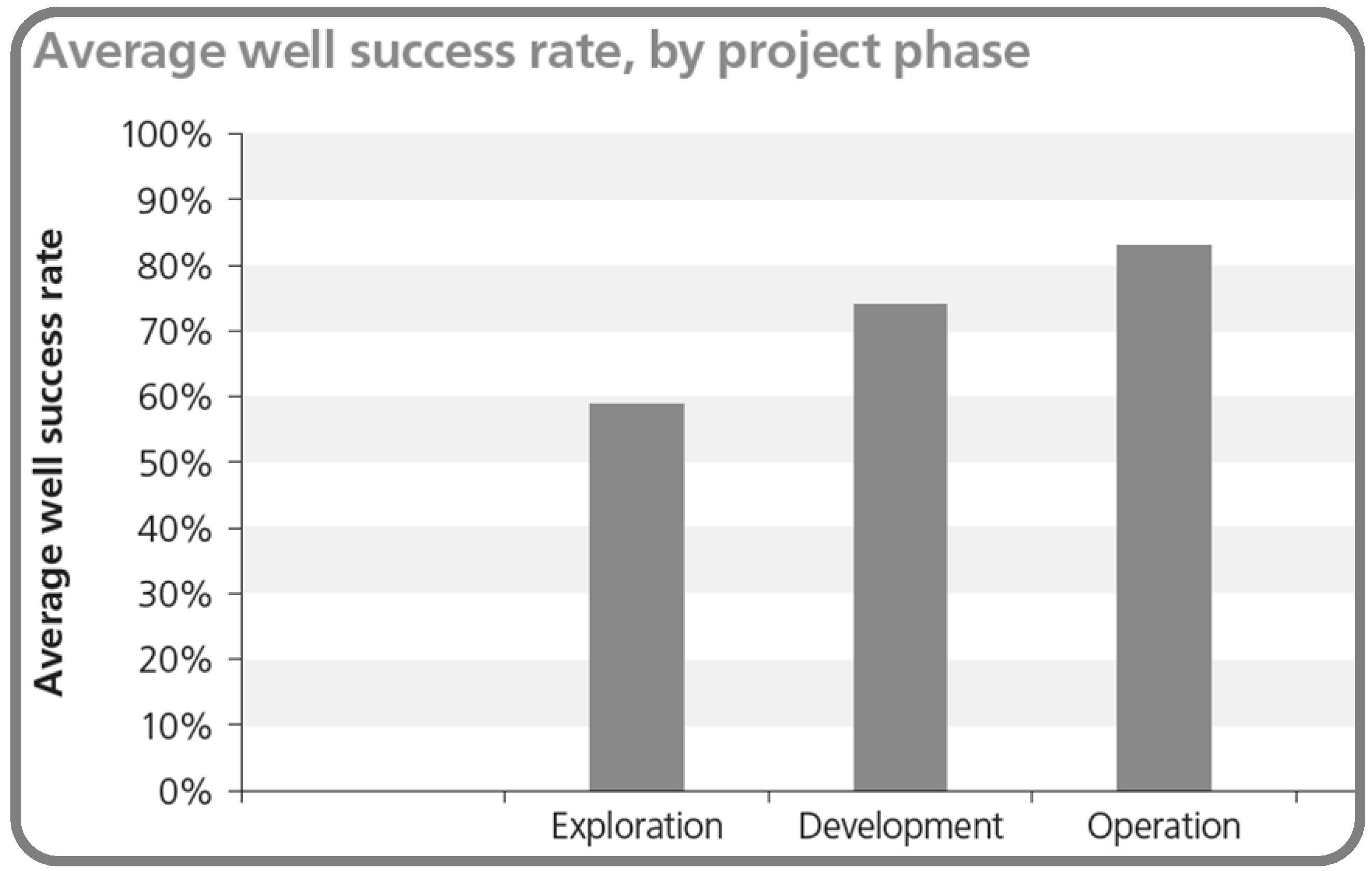
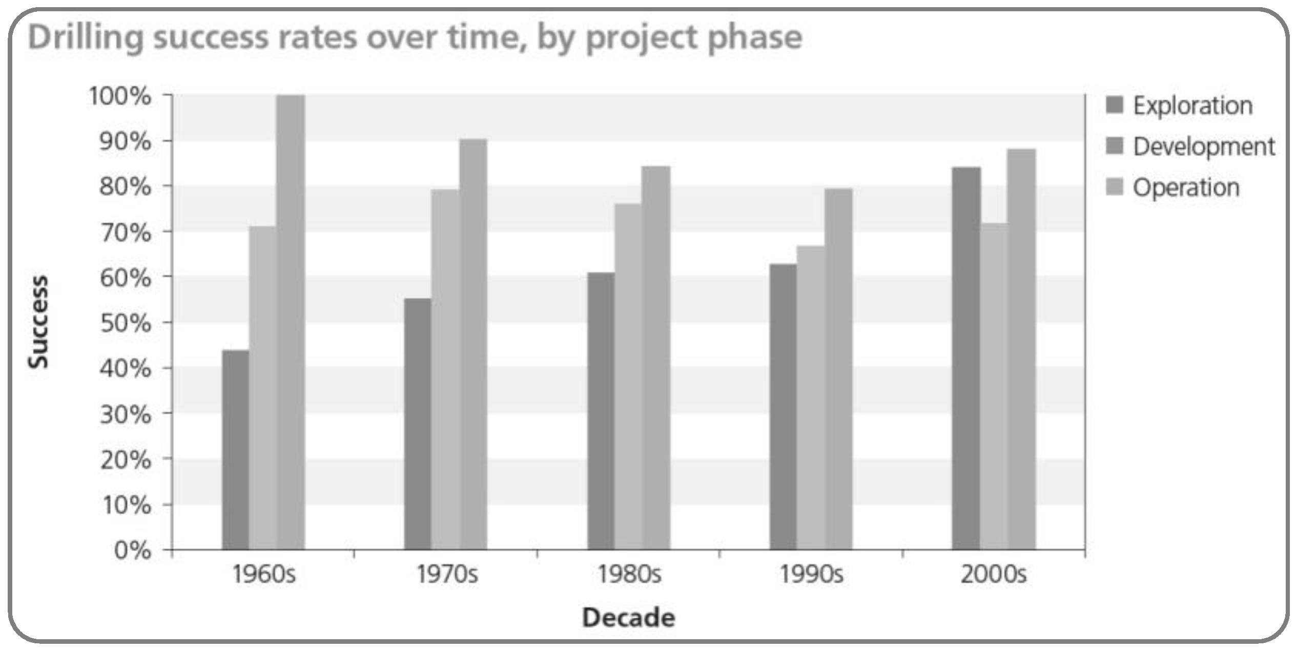
Figure 21.
From the 1960’s to the 2000’s, exploration, development, and operation wells, when averaged together, tend to have a similar success rate of about 70-80%. The lack of greater improvement between exploration and development or operation wells indicates risk factors that are not being mitigated greatly with pre-drill derisking techniques.
A key aspect of any failure analysis is to define success. Importantly, IFC (2013) noted “a dry well is a rarity—almost all wells flow to some extent”. and “a well was deemed to have been successful only where the capacity was above a certain threshold” [29]. This threshold varied widely between the examples analysed, so discussions of success are not historically occurring around standardised criteria. There are other ambiguities. For example, an injection well might be judged as successful on the basis that it is long active, even if was converted from an originally failed production well. It is also relevant to ask whether a well that was originally drilled for electricity, but is instead used for heat due an inadequate temperature, is a failure or a success? Is technical failure defined by the success of the original intended use or the ultimate actual use? Our study assumes the former, i.e., the original use. Any “recovery” of an initial failure is in this philosophy deemed a separate, different project. This is a key observation, as it implies any estimate of geological success (Pg) is a function of end-use. Such ambiguities can interfere with clear interpretation of success case statistics.
According the IFC (2013) study [29], the key reasons for a lack of geothermal success are listed as:
- Mechanical problems during drilling
- Inadequate temperature
- Inadequate pressure
- Insufficient reservoir permeability—too low a production index (PI)
- Unacceptable chemistry—i.e.,: too gassy (not condensable gas), corrosive, or scale prone.
Of those key reasons, mechanical problems during drilling should be disregarded because it relates to the operational risk. Such risk is mitigated taking in account a reasonable “contingency” cost of the well to cope with any unexpected mechanical problem.
We consider the inadequate reservoir pressure a very important factor but not a key one. It could be due to a low reservoir permeability, resulting in low recharge and an early pressure decline. According to the proposed workflow such event is captured in the well deliverability uncertainty and not in the risk. Often, a lower production flow rate per well would prevent such pressure decline.
In short, the approach outlined in this paper addresses a longstanding issue within geothermal development, of standardising treatment of both geothermal geological and commercial success., usefully and necessarily contextualising it in terms of geothermal energy usage.
Appendix B: Historical Resource Assessment Methodologies
Ciriaco et al., 2020, Falcone et al., (2013) and Breede et al., (2015) provide a good overview of the existing methodologies for assessing geothermal resources and reserves and relationship to the UN resources classification system [40,41,42]. Two resource assessment approaches are worth discussing here: the power density method and the volumetric or stored heat method. Each classification reporting system has embedded the concept of resource uncertainty (e.g., proven, probable and possible) and the risk element (exploration and appraisal; resources and reserves). Since 2010, a unified UN sanctioned system has been proposed [10,11,12,43,44,45] providing a unique single scheme of resource reporting that also encompasses geothermal resources. The UN system is a major step forward and the subsection 5.1.3. addresses how the proposed approach can be integrated into it to assist its implementation.
1. Power Density
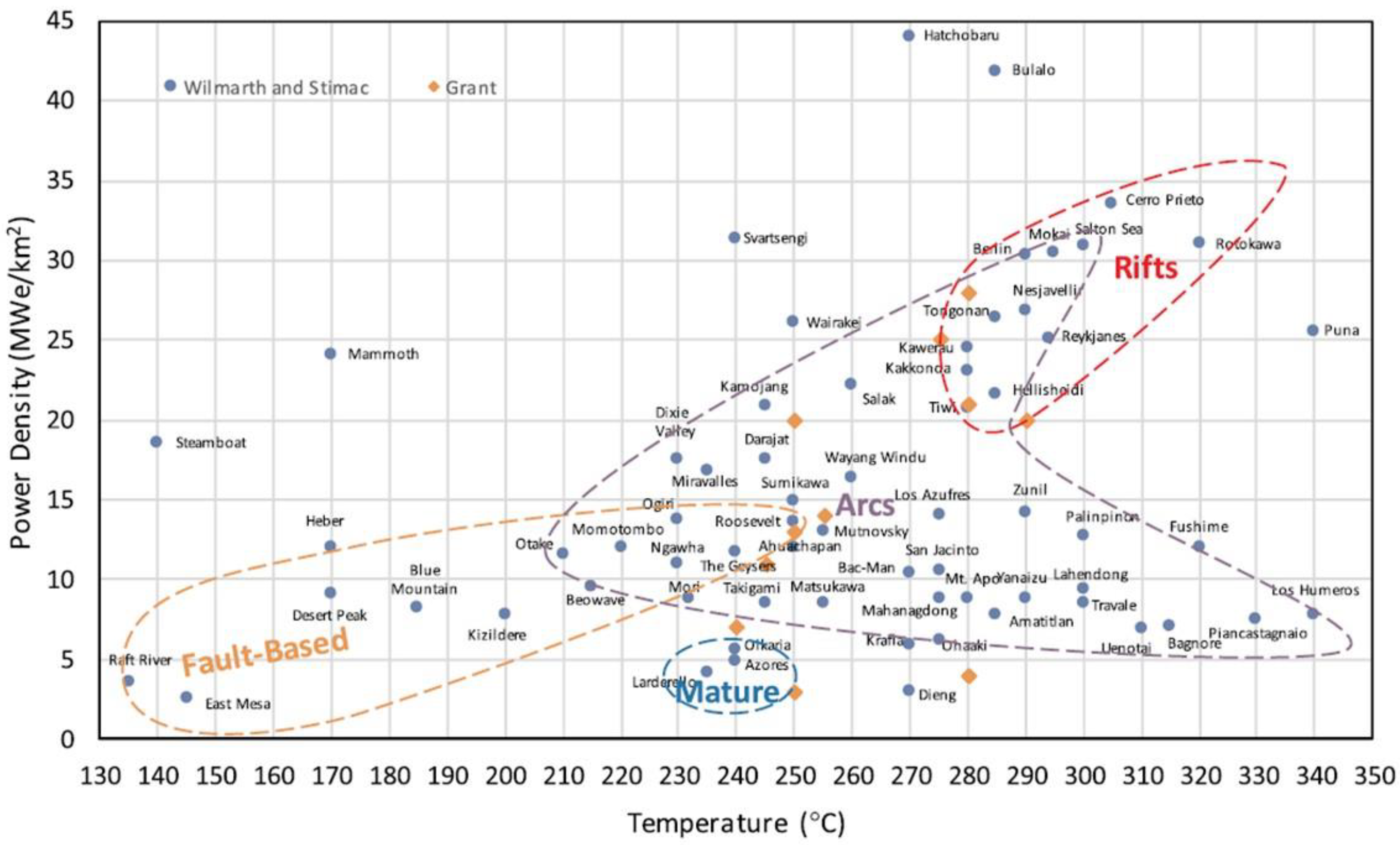
The power density method assumes that the power capacity per unit area MWe/km2 of the productive resource is a function of an initial reservoir temperature Ti (Figure 22) [46,47]. Key implicit assumptions are the production area and the average temperature, including variations in time and space. The method is empirical in that it derives a power density from observed temperatures, areas and usable energy production, rather than theoretically from first principles of subsurface knowledge. Neither does it explicitly incorporate power plant efficiency variations (only net power production figures are used), nor reduced outputs associated with any “non-pay” acid fluids or gas, present in some fields. The empirical inputs capture these implicitly. The method has caveats that should be understood, but it is powerful in simplicity to use for sensible “range” setting—i.e., conditioning certain development scenarios. While the method was instigated for use with power generation plants, the principes are equally applicable direct heat-use applications.
Figure 22.
Power density of high temperature geothermal fields [45,47]. Each “group” of data categorised by tectonic setting and/or field maturity can be used to define appropriate power density probability distribution functions for a region. The power density method is not suitable for assessing the risks and uncertainties of a particular geothermal project, which requires in-depth analysis of an individual field.
2. Volumetric—Heat-in-place Method
The USGS volumetric heat-in-place method (VHIP) considers the total thermal energy that is present in a volume of rock obtainable through its cooling [48,49,50]. Using equipment of a certain thermodynamic efficiency, the resource temperature is cooled to a “reference temperature” and the energy used to generate electricity. This reference temperature is typically assumed to be the abandonment temperature. To assume otherwise (e.g., ambient temperature) would overestimate power generation potential. The system is considered closed, with no heat entering or leaving the system boundary, so that the total energy potential is finite, but the availability of water is infinite. The limiting factor in this model is the resource temperature. Permeability is not considered explicitly but is included in an indirect “heat recovery factor”.
The relationship between the heat recovery factor and the permeability can be understood by analysing the case of an enhanced geothermal system (EGS) deploying artificially engineered fracture permeability. Prior to fracturing, the heat recovery factor of an EGS is virtually zero because there is no heat transport system connecting the reservoir to the surface. The heat recovery factor will progressively increase as the extensiveness and efficiency of the heat transport system through the wells and fracturing increases. Therefore, permeability (natural or induced) is a key parameter affecting the heat recovery factor, although it is often neglected.
In our view, this methodology is most appropriate for evaluating the total geothermal “yet to find” resource of a geological province. At the local project scale, some of the required parameters, such as the heat recovery factor, are difficult to estimate. It also assumes infinite water availability whereas in most cases, water availability is a function of the permeability of the reservoir. In general, the well flow rate is the parameter that has the greatest impact on the uncertainties of the geothermal project, so presuming unlimited water availability is to ignore one of the most important parameters. For this reason, an additional approach, such as that which REM furnishes, is required at a project level of resolution.
3. UN Classification.
Independent attempts to standardise geothermal resource assessment and classification have evolved historically, including within the US, Canada, Australia, and Europe [50,51,52,53,54]. Between 2010 and 2021 they reached an increasing degree of international standardisation [55,56]—following co-operation between the UNECE (United Nations Economic Commission for Europe) and the IGA (International Geothermal Association). This has delivered a series of geothermal updates and supplements to the UNFC (United Nations Framework Classification for Resources [10,11,12,48,49]. The UNFC approach is most concerned with standardised reporting, and categorisation of resources with respect to three axes:
- Economic, environmental and social viability (E axis)
- Degree of confidence (G axis)
- Technical feasibility and maturity (F-axis).
Subdivisions of each axis allow 36 individual permutations of “EFG” classification via the approach.
References
- Gambini, R., Waters, D., Sansone, F., Memmo, V. (2025). Risk and Uncertainty assessment for geothermal projects using Reverse Enthalpy Methodology. European Geothermal Congress 2025—EGEC 2025 Zurich, Switzerland 6-10 October 2025.
- Agemar, T., Weber, J., & Moeck, I. S. (2018). Assessment and public reporting of geothermal resources in Germany: Review and outlook. Energies, 11(2). [CrossRef]
- Frey, M., Bär, K., Stober, I., Reinecker, J., van der Vaart, J., & Sass, I. (2022). Assessment of deep geothermal research and development in the Upper Rhine Graben. In Geothermal Energy (Vol. 10, Issue 1). Springer Science and Business Media Deutschland GmbH. [CrossRef]
- Mendrinos, D., Karytsas, C., & Georgilakis, P. S. (2008). Assessment of geothermal resources for power generation Centre for Renewable Energy Sources and Saving Assessment of geothermal resources for power generation. In Article in Journal of Optoelectronics and Advanced Materials (Vol. 10, Issue 5). Available online: https://www.researchgate.net/publication/228840328.
- Westphal, D., & Weijermars, R. (2018). Economic appraisal and scoping of geothermal energy extraction projects using depleted hydrocarbon wells. Energy Strategy Reviews, 22, 348–364. [CrossRef]
- Maury, J., Hamm, V., Loschetter, A., & Le Guenan, T. (2022). Development of a risk assessment tool for deep geothermal projects: example of application in the Paris Basin and Upper Rhine graben. Geothermal Energy, 10(1), 26. [CrossRef]
- Moghaddam, M. K., Samadzadegan, F., Noorollahi, Y., Sharifi, M. A., & Itoi, R. (2014). Spatial analysis and multi-criteria decision making for regional-scale geothermal favorability map. Geothermics, 50, 189–201. [CrossRef]
- Witter, J. B., Trainor-Guitton, W. J., & Siler, D. L. (2019). Uncertainty and risk evaluation during the exploration stage of geothermal development: A review. In Geothermics (Vol. 78, pp. 233–242). Elsevier Ltd. [CrossRef]
- SPE, WPC, AAPG, SPEE, SEG, EAGE, SPWLA (2018). PRMS Petroleum Resources Management System Revised June 2018 (v. 1.03).
- UNECE. (2010). United Nations Framework Classification for Fossil Energy and Mineral Reserves ECE Energy Series No. 39.
- UNECE. (2017). Application of the United Nations Framework Classification for Resources (UNFC) to geothermal energy resources: selected case studies.
- UNECE, & IGA. (2016). Specifications for the application of the UN Framework Classification for Fossil and Mineral Reserves and Resources 2009 to Geothermal Resources. Available online: http://www.unece.org/fileadmin/DAM/oes/MOU/2014/MoU-UNECE_IGA.pdf.
- Suslick, S. B., & Schiozer, D. J. (2004). Risk analysis applied to petroleum exploration and production: An overview. Journal of Petroleum Science and Engineering, 44(1–2), 1–9. [CrossRef]
- Rose, P. R. (2001). Risk Analysis and Management of Petroleum Exploration Ventures (AAPG methods in Exploration Series)) (Vol. 12). AAPG.
- De Finetti, B.. (1990). The Theory of Probability, Volume 2. John Wiley & Sons Ltd.
- Limpert, E., Werner, A. S., & Abbt, M. (2001). Log-normal Distributions across the Sciences: Keys and Clues. BioScience, 51(5). Available online: http://stat.ethz.ch/vis/log-normal.
- Cook, M. (2021). Petroleum Economics and Risk Analysis: A Practical Guide to E&P Investment Decision-Making. Elsevier.
- Flechtner, F., & Aubele, K. (2019). A brief stock take of the deep geothermal projects in Bavaria, Germany (2018) Geothermie-Allianz Bayern View project A brief stock take of the deep geothermal projects in Bavaria, Germany (2018). Proceedings, 44th Workshop on Geothermal Reservoir Engineering, Stanford, California. Available online: https://www.researchgate.net/publication/334560554.
- Guiling, W., Wenjing, L., Wei, Z., Jiyun, L., & Wanli, W. (2023). Evaluation of Geothermal Resources Potential in China. Proceedings, 48th Workshop on Geothermal Reservoir Engineering, Stanford University, California.
- Mijnlieff, H. F. (2020). Introduction to the geothermal play and reservoir geology of the Netherlands. Netherlands Journal of Geosciences, 99. [CrossRef]
- Breede, K., Dzebisashvili, K., Liu, X., & Falcone, G. (2013). A systematic review of enhanced (or engineered) geothermal systems: past, present and future. In Geothermal Energy (Vol. 1, Issue 4). SpringerOpen. [CrossRef]
- Olasalo, P., Juarez, M. C., Morales, M. P., D’Amico, S., & Liarte, I. A. (2016). Renewable and Sustainable Energy Reviews. [CrossRef]
- Sharmin, T., Khan, N. R., Akram, M. S., & Ehsan, M. M. (2023). A State-of-the-Art Review on Geothermal Energy Extraction, Utilization, and Improvement Strategies: Conventional, Hybridized, and Enhanced Geothermal Systems. In International Journal of Thermofluids (Vol. 18). Elsevier B.V. [CrossRef]
- Combs, J. (2006). Historical Exploration and Drilling Data from Geothermal Prospects and Power Generation Projects in the Western United States. GRC Transactions, 30, 387–392.
- Sanyal, S. K., & Morrow, J. W. (2012). Success and the Learning Curve Effect in Geothermal Well Drilling—A Worldwide Survey. Proceedings, Thirty-Seventh Workshop on Geothermal Reservoir Engineering.
- Schumacher, S., Pierau, R., & Wirth, W. (2020). Probability of success studies for geothermal projects in clastic reservoirs: From subsurface data to geological risk analysis. Geothermics, 83. [CrossRef]
- Shevenell, L. (2012). Rate of Success of Geothermal Wells Nevada. GRC Transactions, 36.
- Wall, A. M., & Dobson, P. F. (2016). Refining the Definition of a Geothermal Exploration Success Rate. Proceedings, 41st Workshop on Geothermal Reservoir Engineering, Stanford University, California.
- IFC. (2013). Success of Geothermal Wells: A Global Study International Finance Corporation.
- Zarrouk, S. J., & Moon, H. (2014). Efficiency of geothermal power plants: A worldwide review. Geothermics, 51, 142-153. [CrossRef]
- Brown, P. J., Rose, P. R. R., Associates, L., & Texas, A. (2001). Plays and Concessions—A Straightforward method for assessing volumes, value, and chance.
- Atkinson, P. G., Celati, R., Corsi, R., & Kucuk, F. (1980). Behavior of the Bagnore Steam/CO2 geothermal Reservoir, Italy. Society of Petroleum Engineers Journal, 20(4), 228–238. [CrossRef]
- Paulillo, A., Striolo, A., & Lettieri, P. (2019). The environmental impacts and the carbon intensity of geothermal energy: A case study on the Hellisheiði plant. Environment International, 133. [CrossRef]
- Gori, F., Barberio, M. D., Barbieri, M., Boschetti, T., Cardello, G. L., & Petitta, M. (2024). Groundwater–rock interactions and mixing in fault–controlled karstic aquifers: A structural, hydrogeochemical and multi-isotopic review of the Pontina Plain (Central Italy). Science of The Total Environment, 951, 175439.
- Boni, C., Bono, P., Calderoni, G., Lombardi, S., Turi, B., 1980. Indagine idrogeologica e geochimica sui rapporti tra ciclo carsico e circuito idrotermale nella pianura Pontina (Lazio meridionale). Geol. Appl. Idrogeol. 15, 203–247. Bari.
- MICA Ministero dell’industria, del commercio e dell’artigianato. (1987). INVENTARIO DELLE RISORSE GEOTERMICHE NAZIONALI. Available online: https://unmig.mase.gov.it/risorse-geotermiche/inventario-delle-risorse-geotermiche-nazionali/ (accessed on 8 November 2024).
- Èubriæ, S., (2012). Basic characteristics of hydraulic model for the Velika Ciglena geothermal reservoir: Nafta 63 5-6. 173-179.
- Guercio, M., & Bonafin, J. (2016, November). The Velika Ciglena geothermal binary power plant. In Proceedings of the 6th African Rift Geothermal Conference, Addis Ababa, Ethiopia (pp. 2-4).
- Gambini,R., Giovani Chiodini, G., Festa, P., Cardellini, C., Benassi, A., Liso, I. S., Tieri, M. (2024). Possible effect of deep CO2 degassing in the formation and development of karst systems. EuroKarst 2024 Rome, 10-14 June.
- Ciriaco, A. E., Zarrouk, S. J., & Zakeri, G. (2020). Geothermal resource and reserve assessment methodology: Overview, analysis and future directions. Renewable and Sustainable Energy Reviews, 119. [CrossRef]
- Falcone, G., Gnoni, A., Harrison, B., & Alimonti, C. (2013). Classification and Reporting Requirements for Geothermal Resources. European Geothermal Congress, Pisa, Italy, 3–7.
- Breede, K., Dzebisashvili, K., & Falcone, G. (2015). Overcoming challenges in the classification of deep geothermal potential. In Geothermal Energy Science (Vol. 3, Issue 1, pp. 19–39). Copernicus GmbH. [CrossRef]
- UNECE. (2013). United Nations Framework Classification for Fossil Energy and Mineral Reserves and Resources 2009: incorporating specifications for its application, ECE Energy Series no. 42.
- UNECE. (2020). United Nations Framework Classification for Resources: update 2019, ECE Energy Series No. 61.
- UNECE. (2022). Supplementary Specifications for the application of the UN Framework Classification for Resources (Update 2019) to Geothermal Energy Resources. Available online: https://unece.org/DAM/oes/MOU/2014/MoU-UNECE_IGA.pdf.
- Cumming, W. (2016). Geothermal Resource Capacity Estimation Using Lognormal Power Density from Producing Fields and Area from Resource Conceptual Models; Advantages, Pitfalls and Remedies Resource Capacity Estimation Using Lognormal Power Density from Producing Fields and Area from Resource Conceptual Models; Advantages, Pitfalls and Remedies. Proceedings, 41st Workshop on Geothermal Reservoir Engineering, Stanford University, California.
- Wilmarth, M., & Stimac, J. (2015). Power Density in Geothermal Fields. Proceedings World Geothermal Congress, 19–25.
- Miyazaki, Y., Tsu, H., Urai, M., Takakura, S.-I., Okubo, Y., & Ogawa, K. (1990). Nationwide Geothermal Assessment in Japan by a Volume Method.
- Watson, A. (2013). Geothermal Engineering, Fundamentals and Applications. Springer.
- Williams, C. F., Reed, M. J., & Mariner, R. H. (2008). A Review of Methods Applied by the U.S. Geological Survey in the Assessment of Identified Geothermal Resources.
- Australian Geothermal Energy Group AGRCC. (2010a). Australian Code for Reporting of Exploration Results, Geothermal Resources and Geothermal Reserves.
- Australian Geothermal Energy Group AGRCC. (2010b). Geothermal Lexicon for Resources and Reserves Definition and Reporting. [CrossRef]
- Lawless, J. V, Ward, M., Beardsmore, G., & Nz, J. C. (2010). The Australian Code for Geothermal Reserves and Resources Reporting: Practical Experience. Proceedings World Geothermal Congress, Indonesia. Available online: http://refhub.elsevier.com/S1364-0321(19)30723-3/sref15.
- Williams, C. F., Reed, M. J., Galanis, S. P., & Deangelo, J. (2007). The USGS national geothermal resource assessment: An update. Proceedings Geothermal Resource Council Transactions 2007, 99–104.
- Falcone, G. (2015). Proposal of a consistent framework to integrate geothermal potential classification with energy extraction. Geothermal Energy Science, 3(1), 7–11. [CrossRef]
- Falcone, G., & Beardsmore, G. (2015). Including Geothermal Energy within a Consistent Framework Classification for Renewable and Non-Renewable Energy Resources. In Proceedings World Geothermal Congress. Available online: https://www.researchgate.net/publication/271769867.
| 1 | if not included in fluid adverse composition threshold PoS or in the development cost as described above. |
Figure 1.
Uncertainty in project resources as captured by probability distribution functions (PDF) and the corresponding cumulative distribution function (CDF). The success case Pg is the chance of falling on the P99 to P01 range. The large-uncertainty and small-uncertainty project share the same mean, but the range of possible outcomes is much greater for the large-uncertainty project.
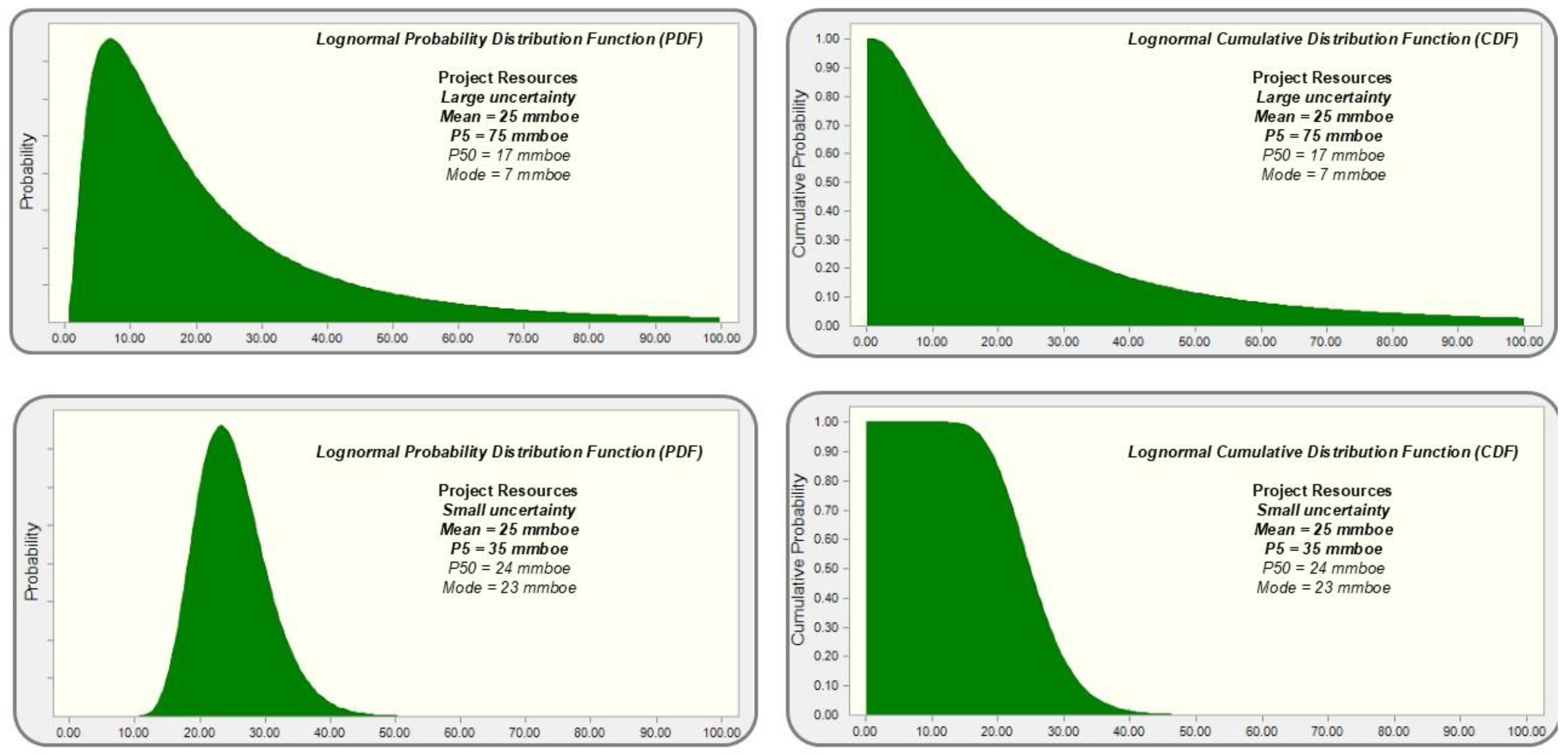
Figure 2.
Application of the Minimum Commercial Field Size (MCFS) to derive commercial success chance (Pc) Modified from Cook, M. (2021) [17].
Figure 2.
Application of the Minimum Commercial Field Size (MCFS) to derive commercial success chance (Pc) Modified from Cook, M. (2021) [17].
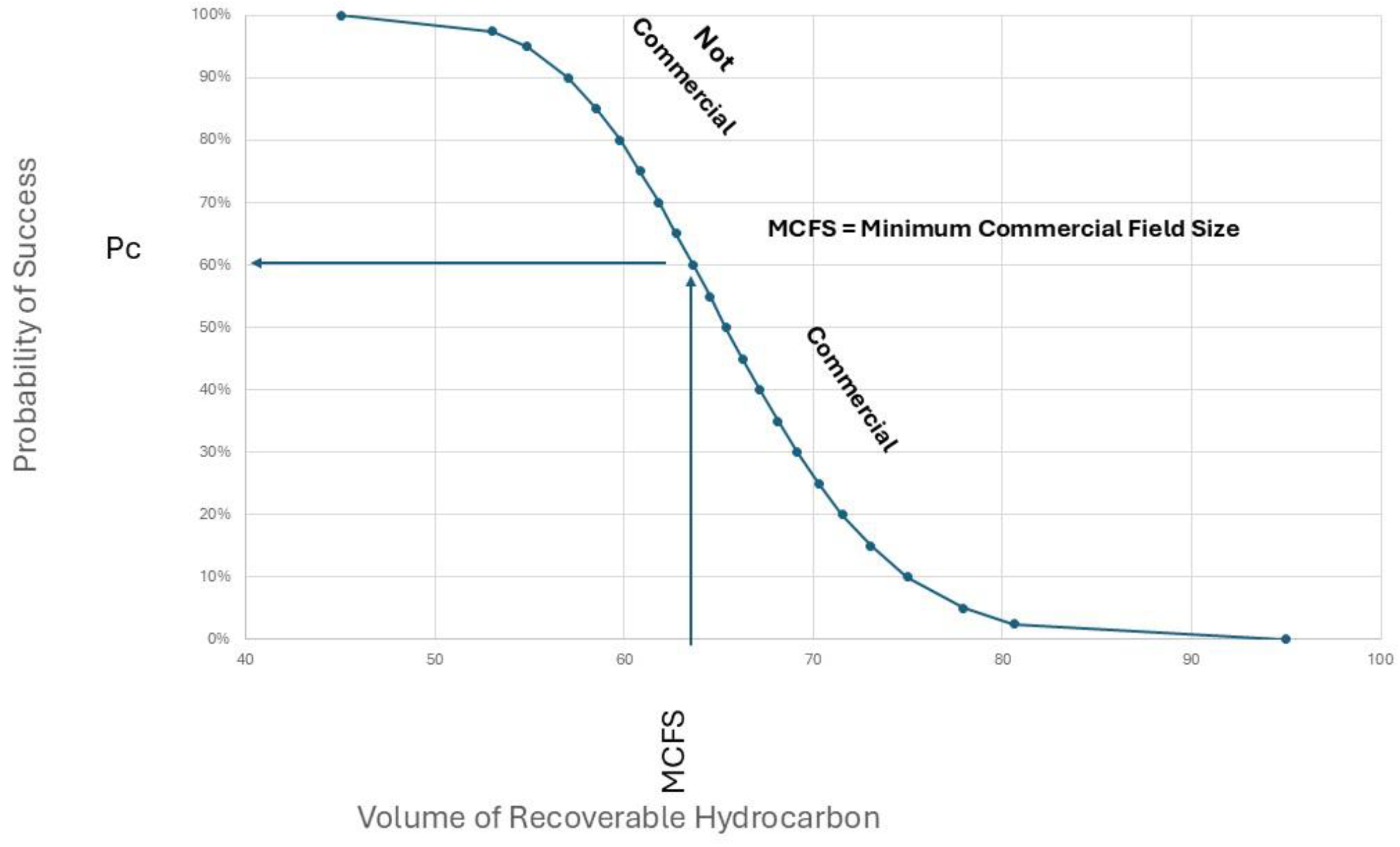
Figure 3.
The geothermal conceptual model showing the elements required for a geothermal field. Illustrated are the Cerro Pabellon binary power plant, Chile, and direct use heat applications in Munich, Germany. Images reproduced with permission of Enel Green Power and SWM respectively.
Figure 3.
The geothermal conceptual model showing the elements required for a geothermal field. Illustrated are the Cerro Pabellon binary power plant, Chile, and direct use heat applications in Munich, Germany. Images reproduced with permission of Enel Green Power and SWM respectively.
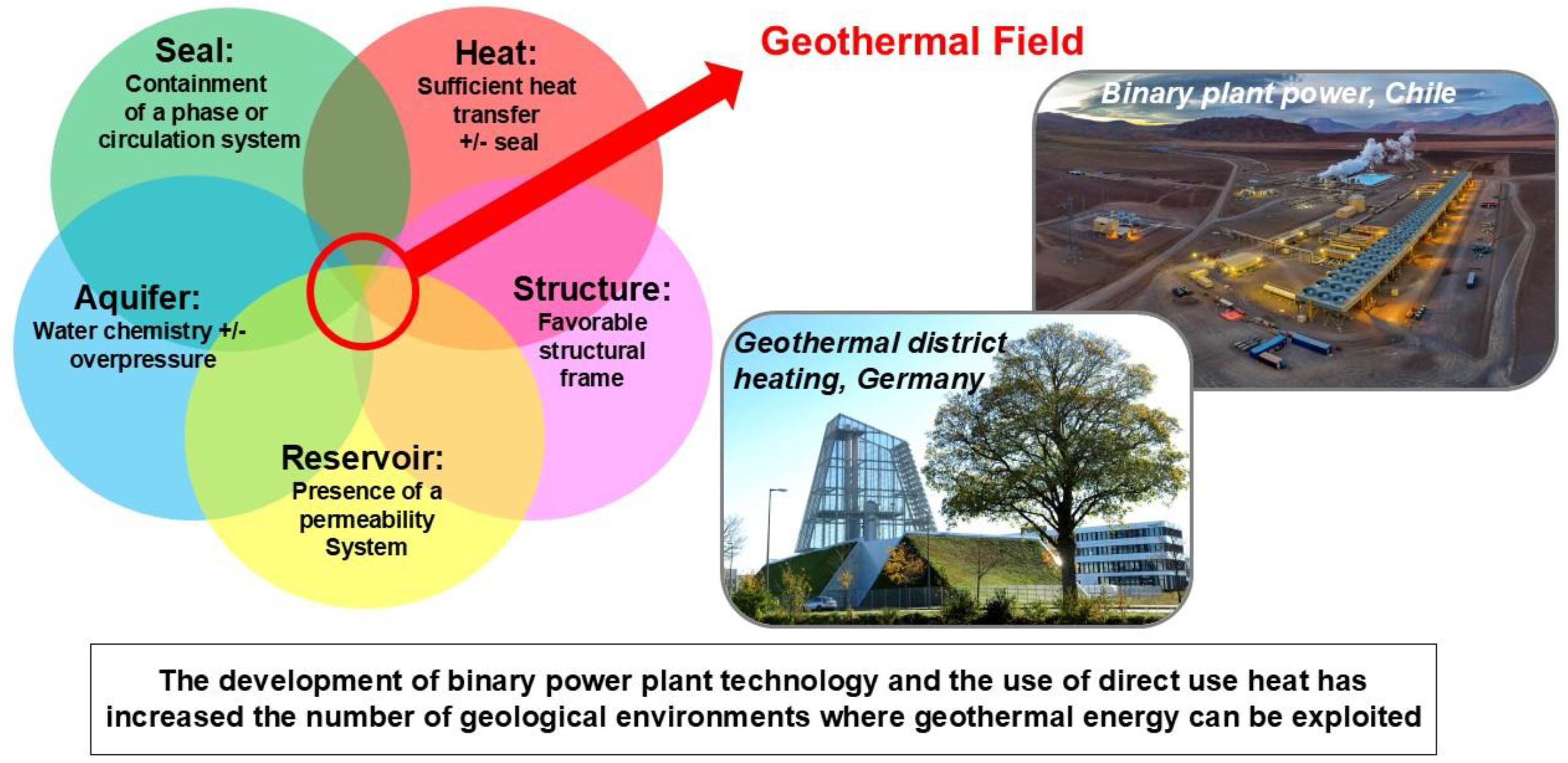
Figure 4.
Typical geothermal development options according to reservoir pressure and temperature conditions. Dry steam, flash, and high enthalpy binary plants dominate the hotter and higher-pressure geothermal fields. Binary plants and direct use applications such as district heating dominate cooler and lower pressure geothermal fields.
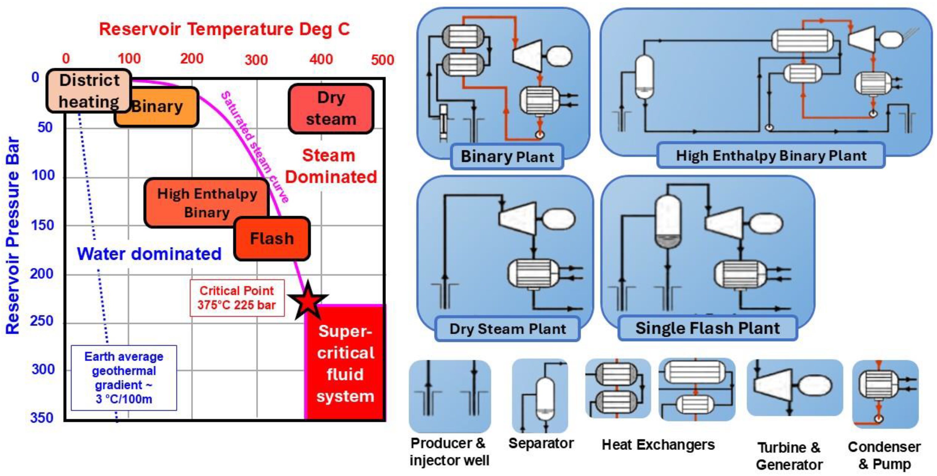
Figure 5.
Conceptual correlation between geothermal fluid temperature and required flow rate for a 20 MW binary power plant. Higher temperature fluids are more efficient at generating electricity than the lower temperature fluids.
Figure 5.
Conceptual correlation between geothermal fluid temperature and required flow rate for a 20 MW binary power plant. Higher temperature fluids are more efficient at generating electricity than the lower temperature fluids.
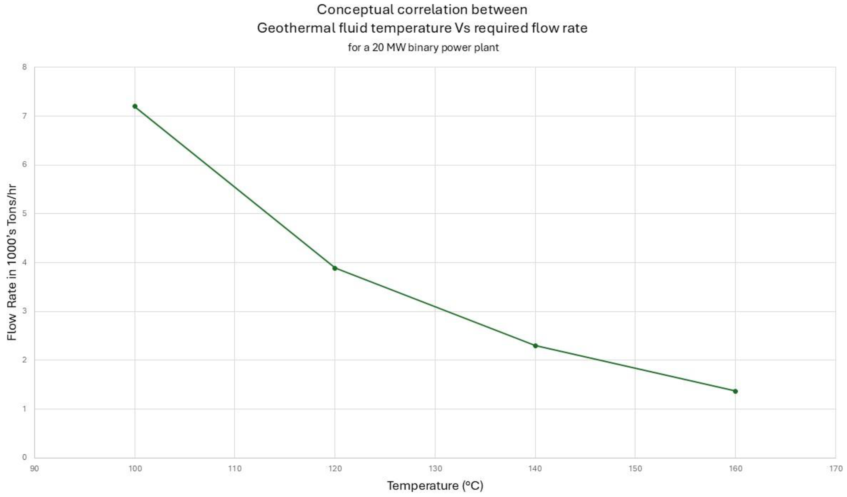
Figure 6.
The binary efficiency function of temperature [30].
Figure 6.
The binary efficiency function of temperature [30].
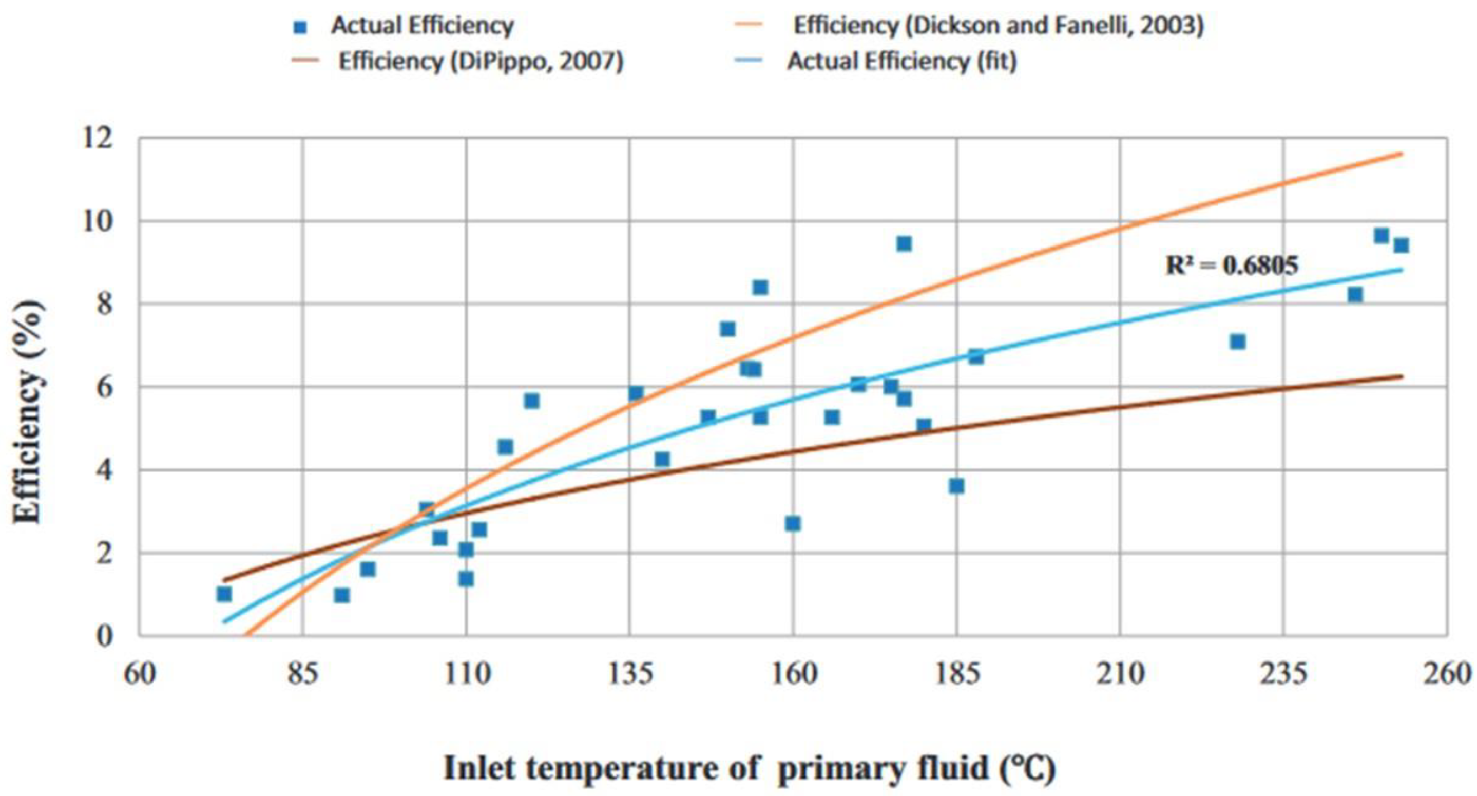
Figure 7.
Conceptual correlation between temperature, binary plant size and plant CAPEX per installed MW.
Figure 7.
Conceptual correlation between temperature, binary plant size and plant CAPEX per installed MW.
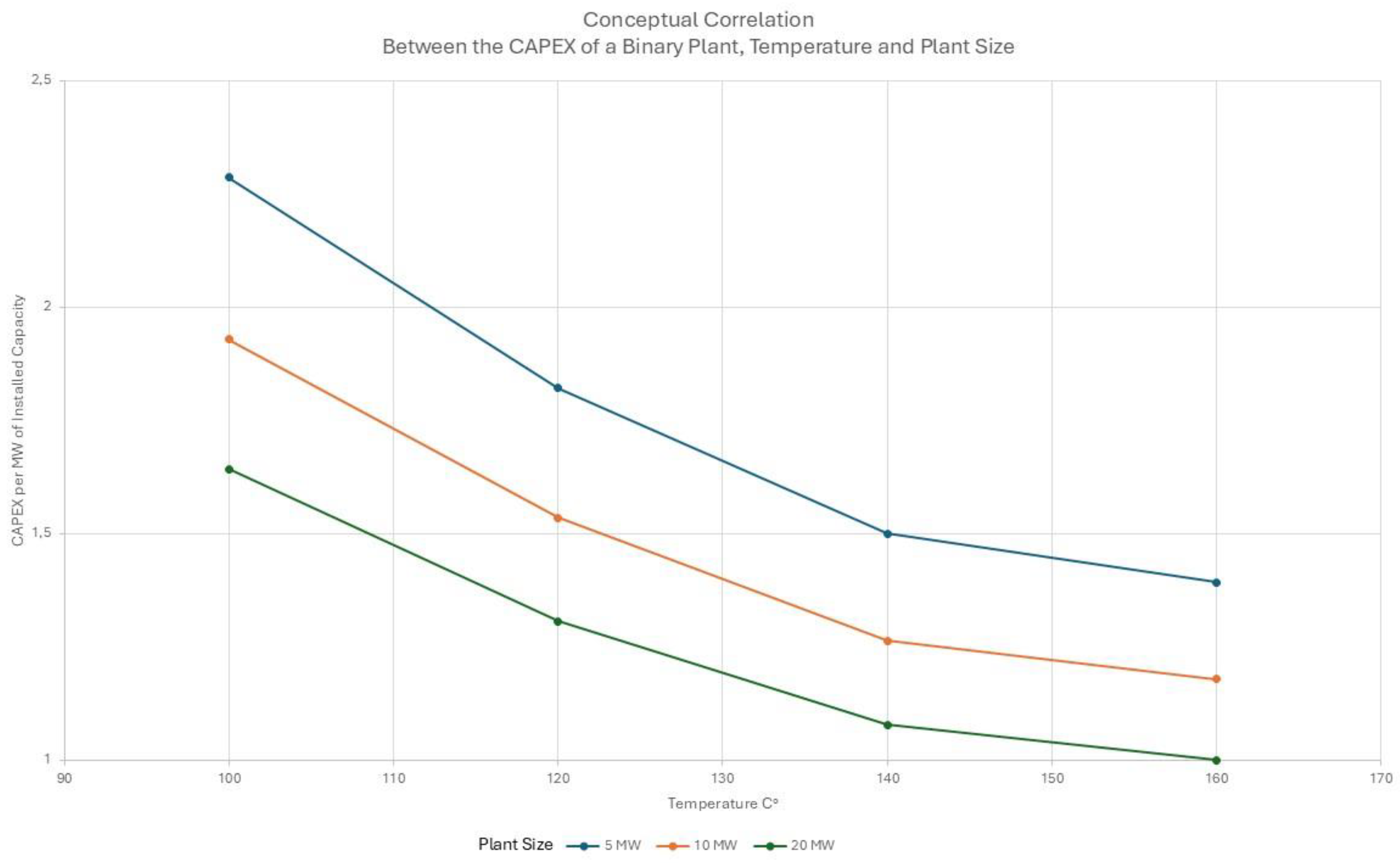
Figure 8.
Geological graphical abstract of the Lepini-Pontina Plain area reprinted from Gori at al 2024.
Figure 8.
Geological graphical abstract of the Lepini-Pontina Plain area reprinted from Gori at al 2024.
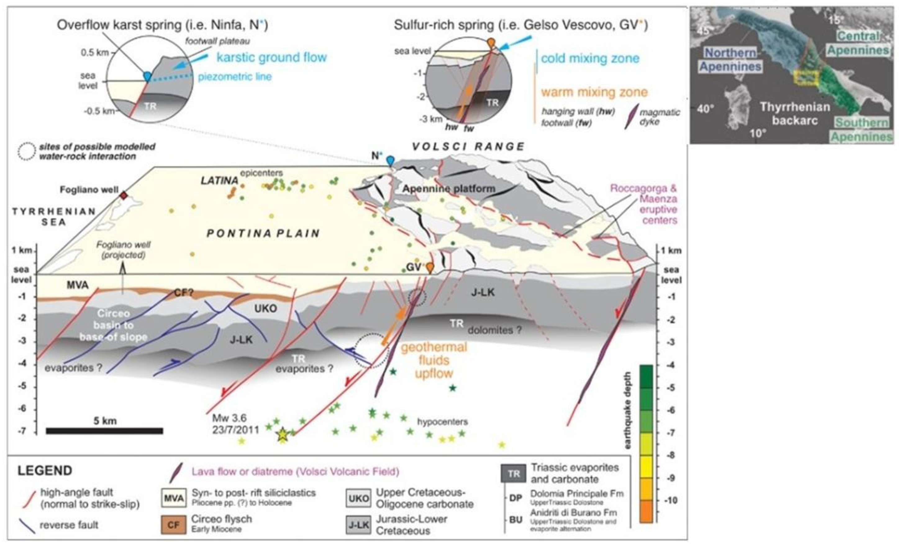
Figure 1.
Geological graphical abstract of the Lepini-Pontina Plain area reprinted from Gori at al 2024.
Figure 1.
Geological graphical abstract of the Lepini-Pontina Plain area reprinted from Gori at al 2024.
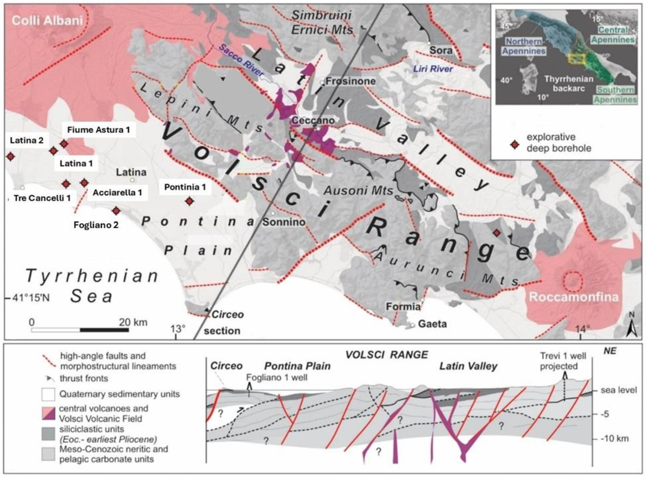
Figure 10.
The relatively high temperature recorded in the Fogliano 2 well, as a combined effect of i) advective deep water circulation due to the high topographic recharge zone of Mt. Lepini and ii) the intra-reservoir convective cycle.
Figure 10.
The relatively high temperature recorded in the Fogliano 2 well, as a combined effect of i) advective deep water circulation due to the high topographic recharge zone of Mt. Lepini and ii) the intra-reservoir convective cycle.
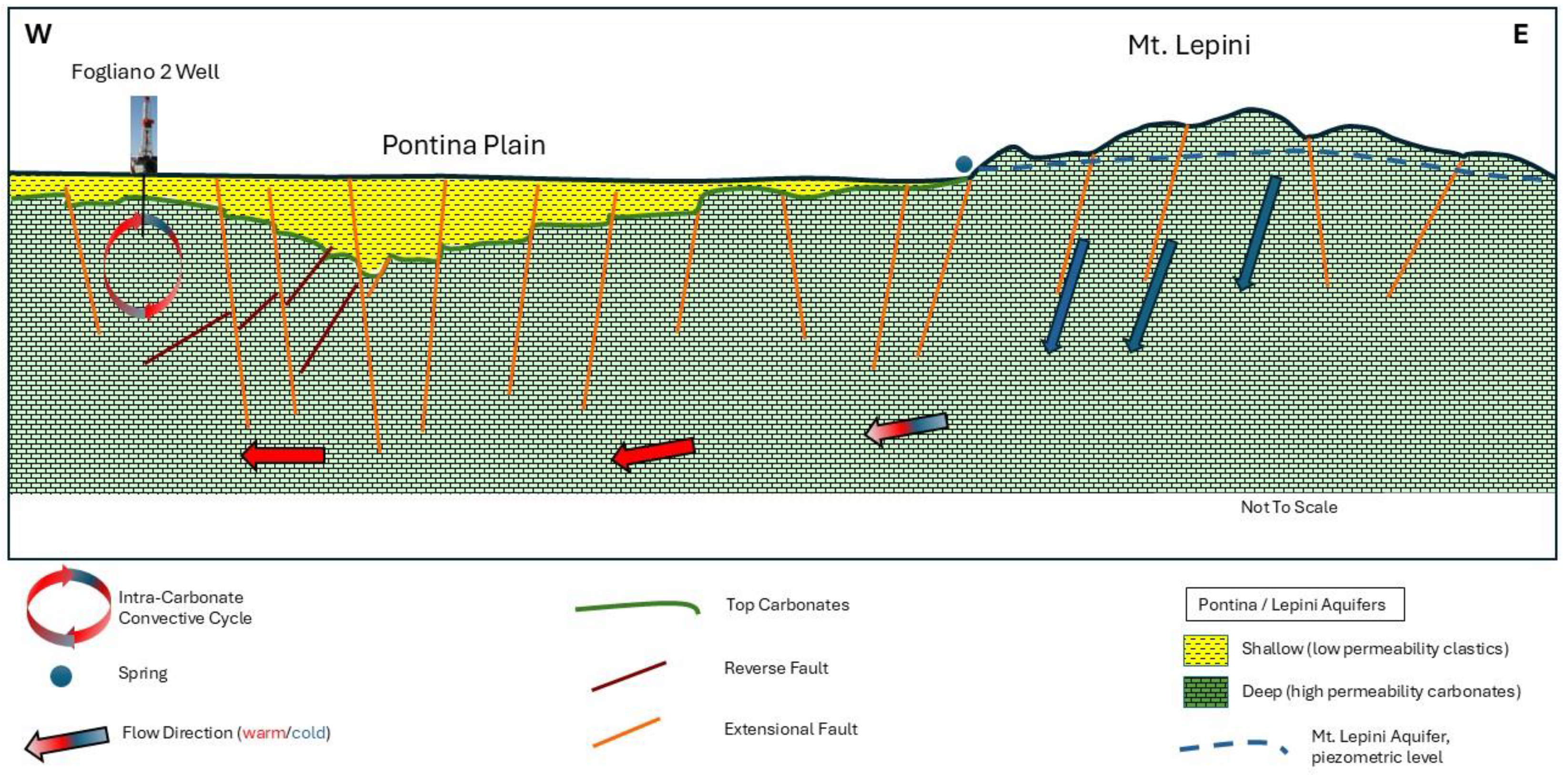
Figure 11.
Geothermal well profiles Acciarella 1 and Latina 2 wells are interpreted to be drilled just above an intra reservoir convective cycle. Latina 1, Tre Cancelli 1 and Fiume Astura 1 Wells are interpreted to have a purely conductive geothermal gradient.
Figure 11.
Geothermal well profiles Acciarella 1 and Latina 2 wells are interpreted to be drilled just above an intra reservoir convective cycle. Latina 1, Tre Cancelli 1 and Fiume Astura 1 Wells are interpreted to have a purely conductive geothermal gradient.
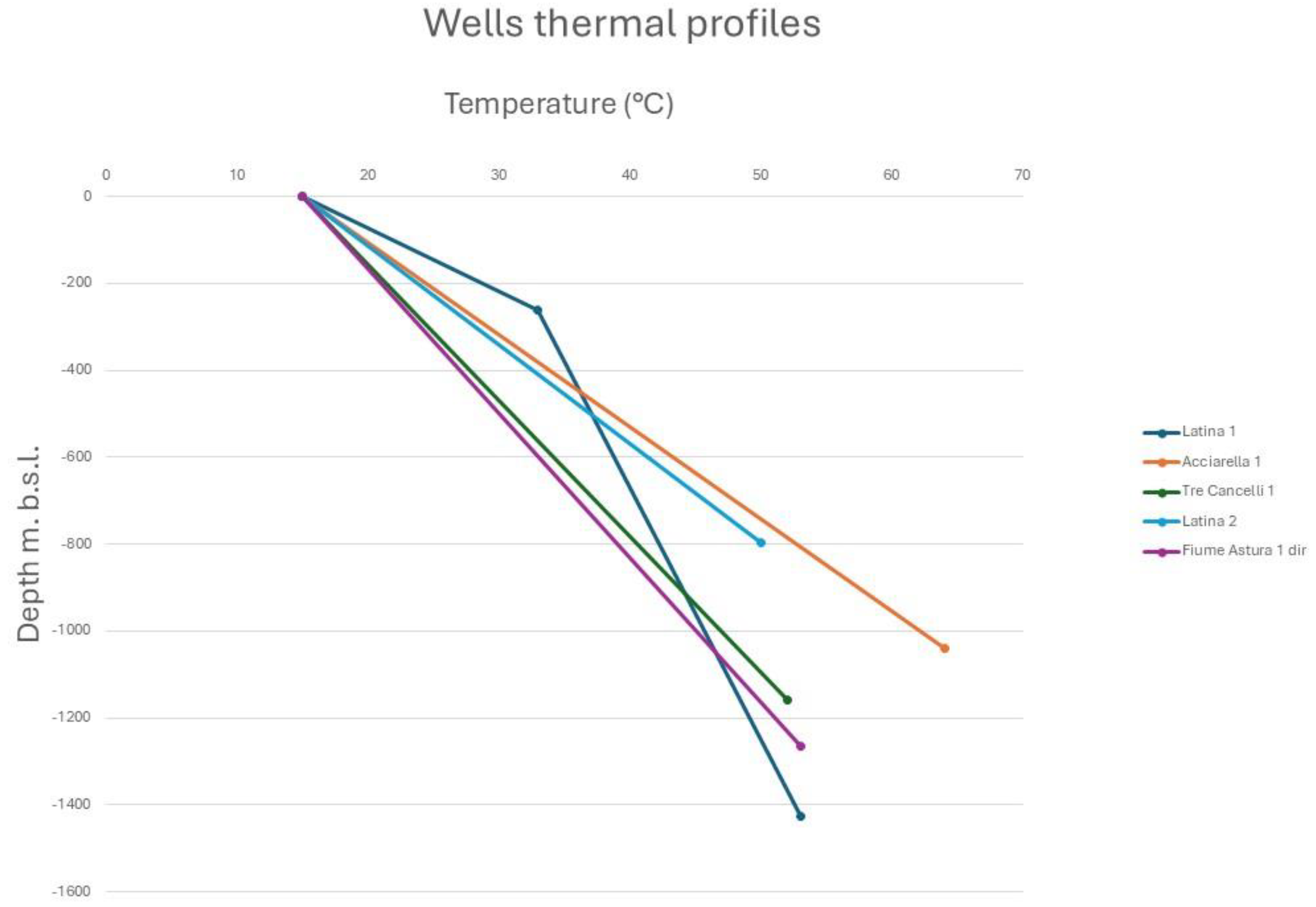
Figure 2.
Geothermal fluid temperature cumulative distribution function of Pontina Plain. Assuming a threshold temperature value of 60 C, the temperature threshold PoS is slightly less than 80%.
Figure 2.
Geothermal fluid temperature cumulative distribution function of Pontina Plain. Assuming a threshold temperature value of 60 C, the temperature threshold PoS is slightly less than 80%.
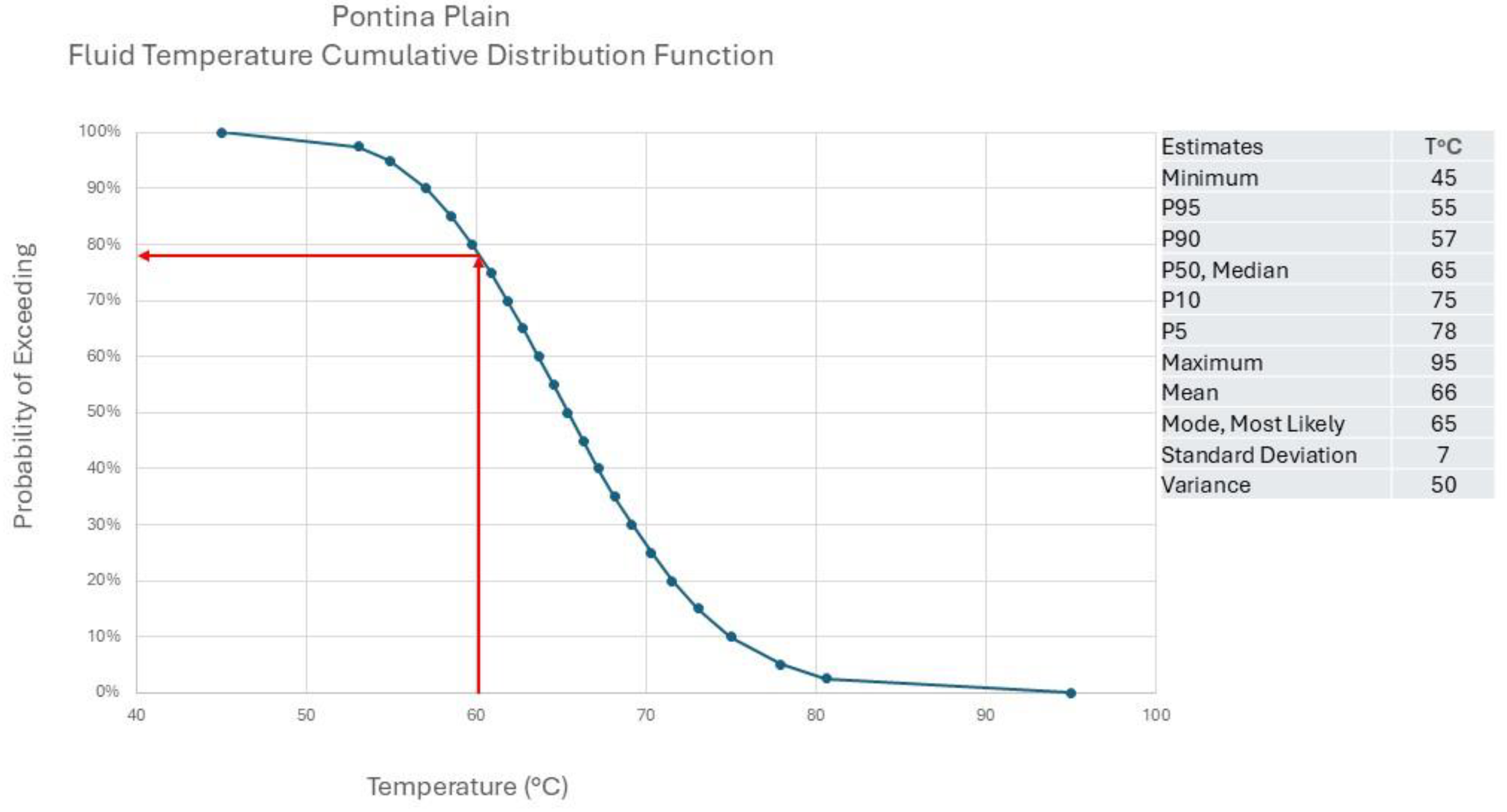
Figure 13.
well deliverability CDF as generated in subsection 5.3.1.
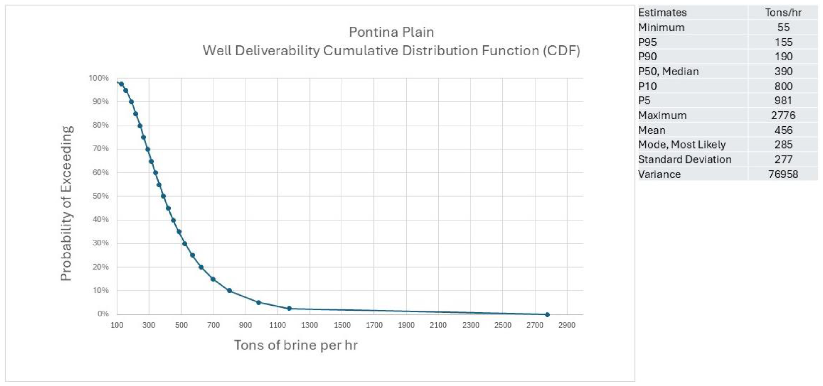
Figure 14.
CDF of the number of production wells needed to supply the chosen plant.
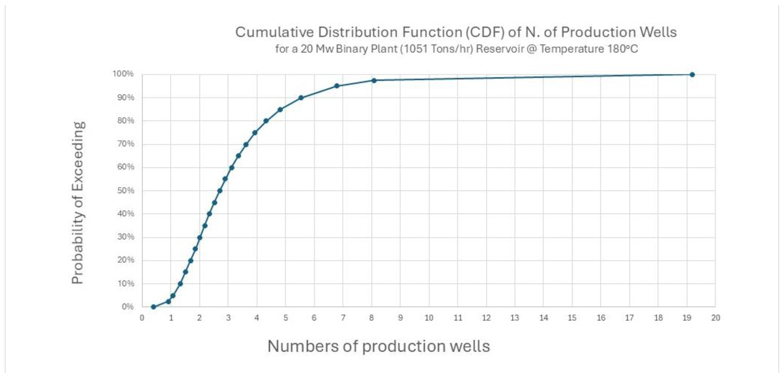
Figure 15.
CDF of the total number of wells (including reinjection and possible abandoned exploration wells).
Figure 15.
CDF of the total number of wells (including reinjection and possible abandoned exploration wells).
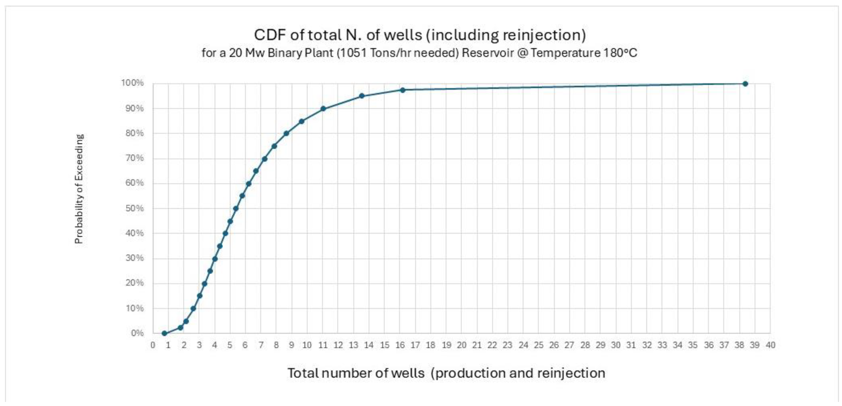
Figure 16.
Knowing the costs of wells, gathering system and related civil works is possible to generate the total drilling related costs CDF to estimate the dPc. In this example, the drilling related cost that makes the NPV of the project equal to zero is €65 million, corresponding to a dPcof 65%.
Figure 16.
Knowing the costs of wells, gathering system and related civil works is possible to generate the total drilling related costs CDF to estimate the dPc. In this example, the drilling related cost that makes the NPV of the project equal to zero is €65 million, corresponding to a dPcof 65%.
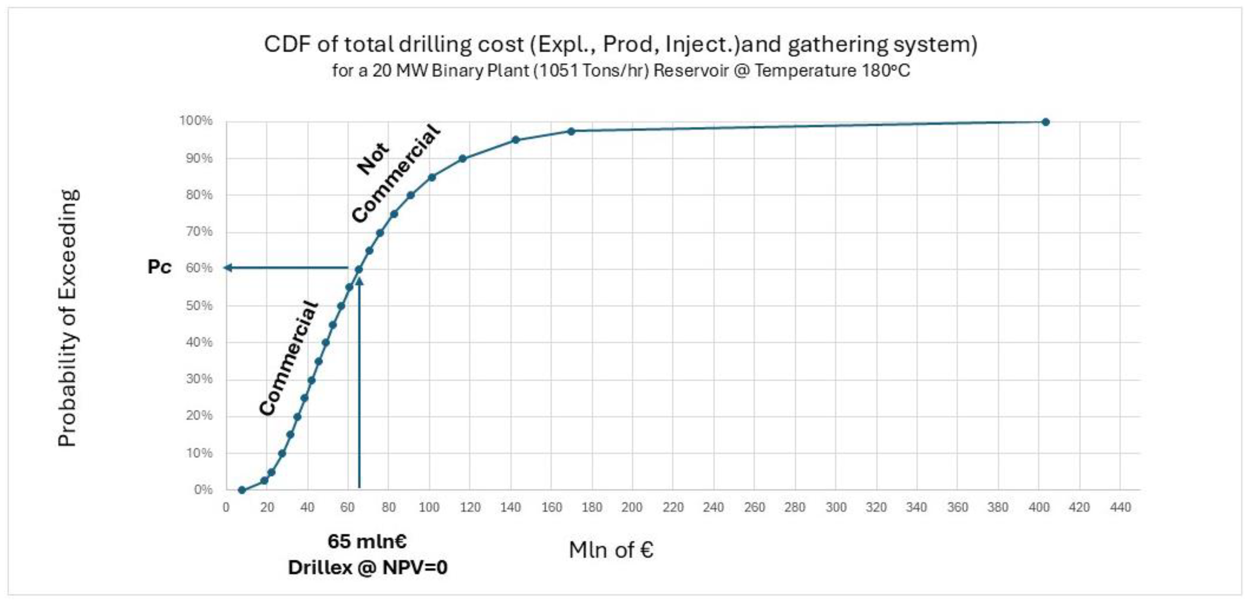
Figure 17.
three well deliverability CDFs aggregated using Montecarlo techniques.
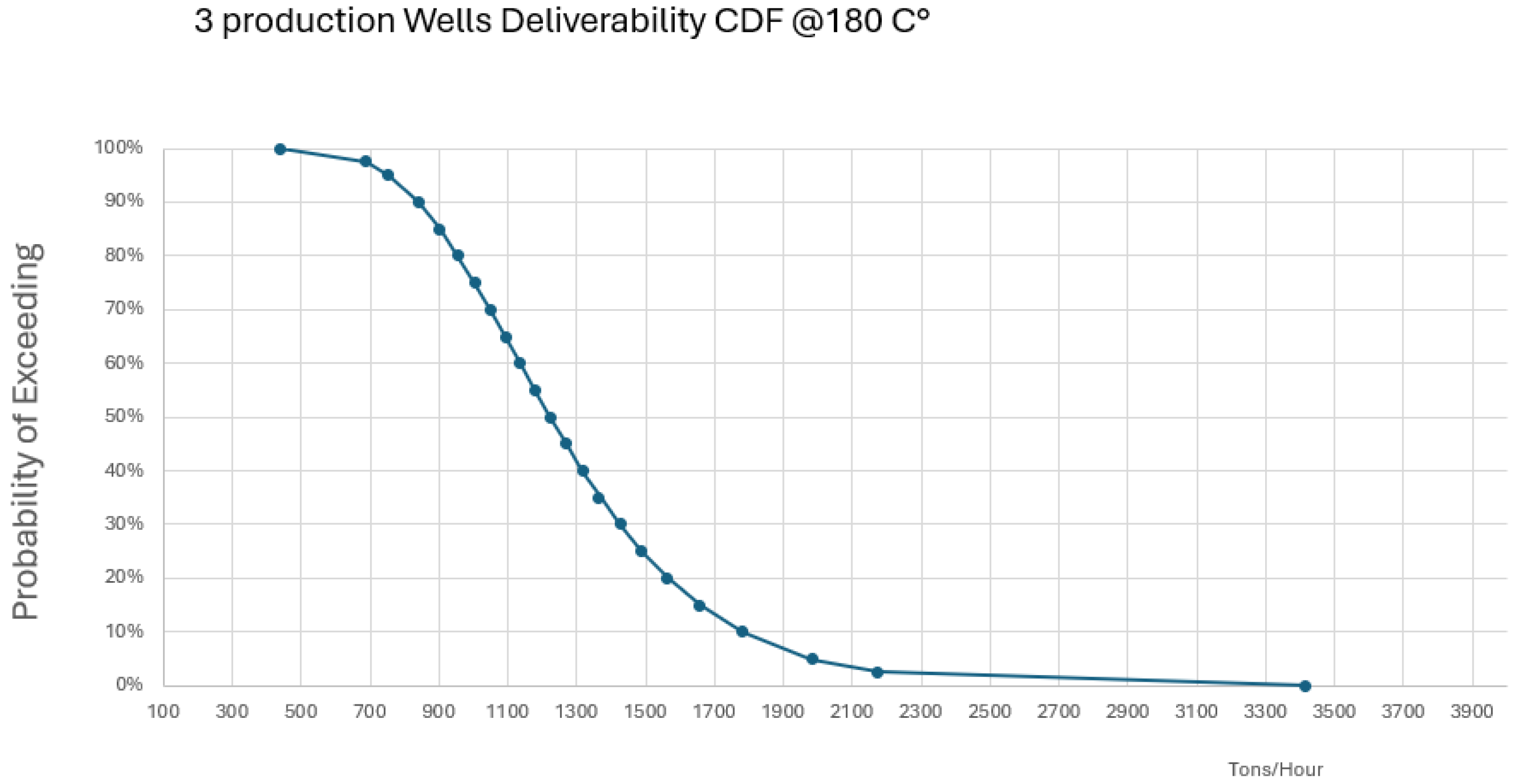
Figure 18.
Estimation of Pcf. Based on the minimum capacity of a geothermal plant that will make the NPV = 0 at the assumed number of production wells.
Figure 18.
Estimation of Pcf. Based on the minimum capacity of a geothermal plant that will make the NPV = 0 at the assumed number of production wells.
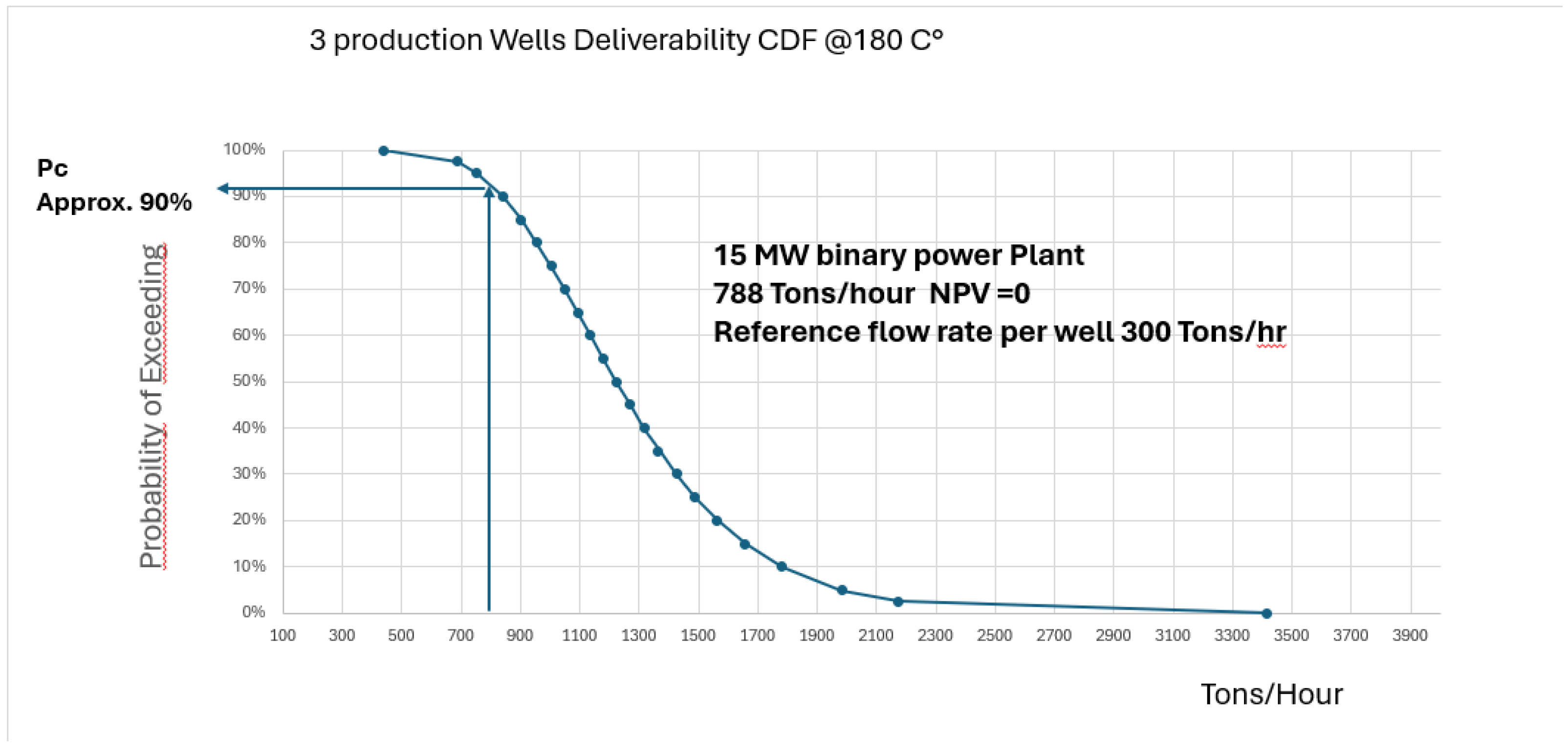
Figure 19.
Categorization of plant capacity uncertainty assuming three production wells. In this example the 20 and 25 MW cases where estimated and then the extrapolated the P50 case.
Figure 19.
Categorization of plant capacity uncertainty assuming three production wells. In this example the 20 and 25 MW cases where estimated and then the extrapolated the P50 case.
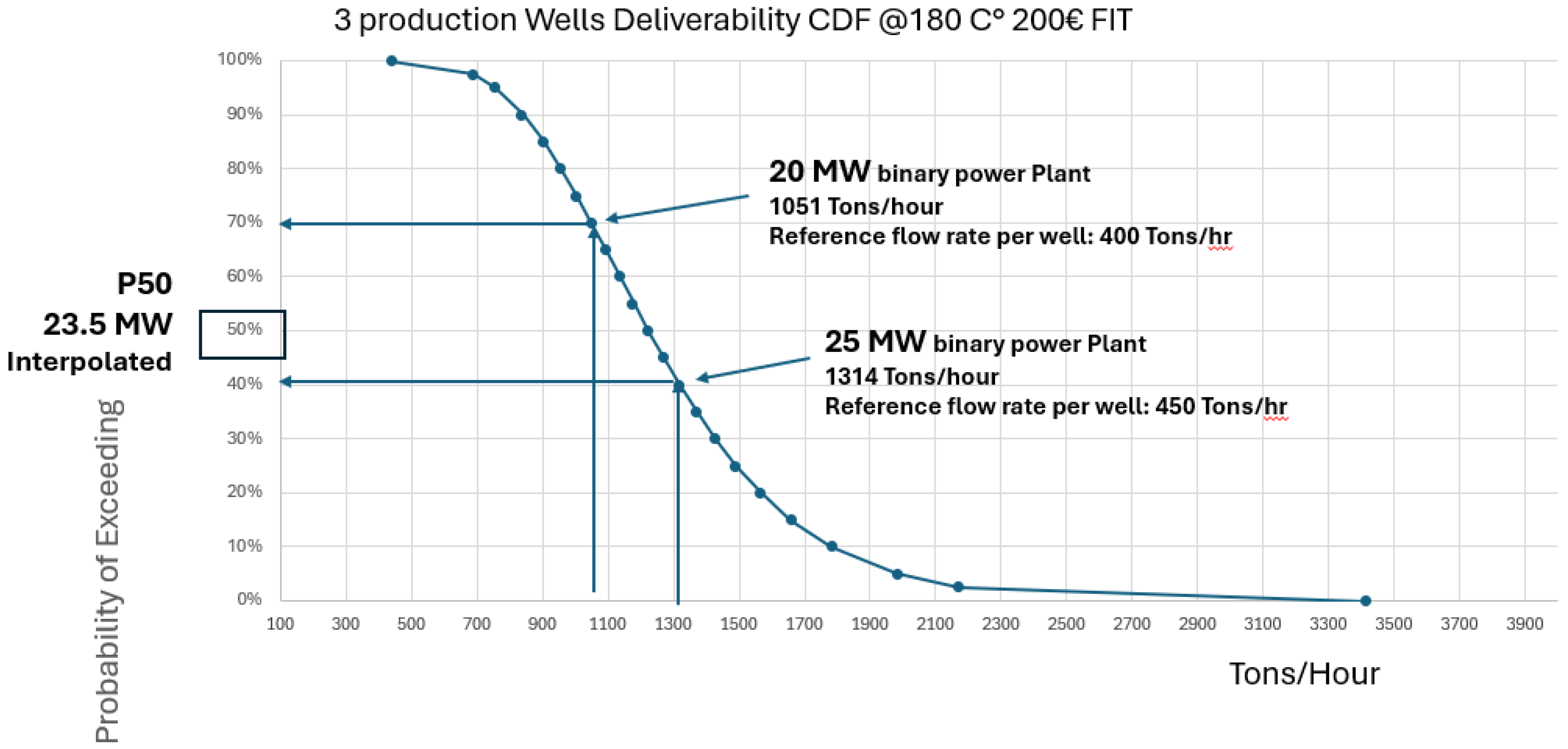
Disclaimer/Publisher’s Note: The statements, opinions and data contained in all publications are solely those of the individual author(s) and contributor(s) and not of MDPI and/or the editor(s). MDPI and/or the editor(s) disclaim responsibility for any injury to people or property resulting from any ideas, methods, instructions or products referred to in the content. |
© 2025 by the authors. Licensee MDPI, Basel, Switzerland. This article is an open access article distributed under the terms and conditions of the Creative Commons Attribution (CC BY) license (http://creativecommons.org/licenses/by/4.0/).
Copyright: This open access article is published under a Creative Commons CC BY 4.0 license, which permit the free download, distribution, and reuse, provided that the author and preprint are cited in any reuse.


