Disproving the Unique Games Conjecture

1. Introduction

The Minimum Vertex Cover (MVC) problem is a fundamental challenge in combinatorial optimization and graph theory. Given an undirected graph, the goal is to find the smallest set of vertices that "covers" every edge—meaning at least one endpoint of each edge is included. Despite its simple formulation, MVC is computationally intractable for large graphs, being one of the first problems proven NP-hard [1]. This status makes it a benchmark for understanding the limits of efficient computation.

While finding an exact solution is impractical for large instances, approximation algorithms offer a practical alternative. A basic greedy approach achieves a 2-approximation—guaranteeing a vertex cover at most twice the optimal size. This result, credited to Gavril and Yannakakis [2], remains a cornerstone of approximation theory. Subsequent work has refined this factor slightly [3,4].

The hardness of approximation for MVC was further cemented by Dinur and Safra (2005), who used the PCP theorem to prove that no polynomial-time algorithm can achieve a ratio better than 1.3606 unless $P=NP$ [5]. Later work tightened this bound to $\sqrt{2}-ϵ$ for any $ϵ>0$ under standard complexity assumptions [6]. Most strikingly, if the Unique Games Conjecture (UGC) holds, then no constant-factor approximation better than 2 is possible [7]. These results highlight the deep theoretical barriers surrounding MVC and the challenges in improving its approximations.

The find_vertex_cover algorithm approximates a minimum vertex cover for an undirected graph $G=(V,E)$ by leveraging the Burr-Erdos-Lovász (1976) method to partition edges into two claw-free subgraphs, computing exact vertex covers for each using the Faenza, Oriolo, and Stauffer (2011) approach in $\mathcal{O}\left(n^3\right)$ time per subgraph, and recursively refining the solution on residual edges [8,9]. With a worst-case runtime of $\mathcal{O}\left(n^4\right)$, where $n=\left|V\right|$, the algorithm achieves an approximation ratio less than 2, improving upon the standard 2-approximation. This method holds potential theoretical impact, challenging the Unique Games Conjecture, while offering practical utility in network design and bioinformatics.

2. State-of-the-Art Algorithms

The Minimum Vertex Cover (MVC) problem, being NP-hard, has been the focus of extensive research, leading to the development of numerous heuristic and approximation algorithms. Recent advancements in this area include:

• Local Search Techniques: Local search methods have emerged as some of the most effective approaches for solving the MVC problem, often outperforming other heuristics in terms of both solution quality and runtime efficiency [10]. Notable algorithms in this category include:

  -

  FastVC2+p: Introduced in 2017, this algorithm is highly efficient for solving large-scale instances of the MVC problem [11].

  -

  MetaVC2: Proposed in 2019, MetaVC2 integrates multiple advanced local search techniques into a highly configurable framework, making it a versatile tool for MVC optimization [12].

  -

  TIVC: Developed in 2023, TIVC employs a 3-improvements framework with tiny perturbations, achieving state-of-the-art performance on large graphs [13].

• Machine Learning Approaches: Reinforcement learning-based solvers, such as S2V-DQN, have shown potential in constructing MVC solutions [14]. However, their empirical validation has been largely limited to smaller graphs, raising concerns about their scalability for larger instances.
• Genetic Algorithms and Heuristics: While genetic algorithms and other heuristics have been explored for the MVC problem, they often face challenges in scalability and efficiency, particularly when applied to large-scale graphs [15].

3. Triangle Detection Algorithm (Aegypti)

3.1. Introduction

The Triangle Detection Problem involves determining whether an undirected graph contains at least one triangle—a set of three vertices where each pair is connected by an edge. This problem is a cornerstone of graph theory with wide-ranging applications, including social network analysis, clustering, and computational biology. The aegypti package offers a novel algorithm for this task, claiming a linear-time complexity of $\mathcal{O}(n+m)$, where n is the number of vertices and m is the number of edges [16]. This efficiency challenges traditional complexity bounds and positions aegypti as a potential breakthrough in graph algorithm design.

The algorithm employs a Depth-First Search (DFS)-based approach, optimized to traverse the graph and identify triangles in a single pass, making it highly efficient for both sparse and dense graphs when validated.

3.2. Algorithm Overview

3.2.1. Key Steps:

• Graph Traversal with DFS: The algorithm initiates a DFS from each unvisited vertex, exploring the graph’s edges systematically to detect potential triangular structures.
• Triangle Identification: During traversal, it checks for a closing edge (e.g., from a parent to a neighbor) that completes a triangle. This is achieved by maintaining parent-child relationships in the DFS stack.
• Early Termination (Optional): For the decision version, the algorithm can stop upon finding the first triangle, while the listing version continues to identify all triangles.

3.2.2. Output:

Returns a list of sets, where each set contains three vertices forming a triangle, or None if no triangles are found. With the first_triangle=True parameter, it returns after the first triangle is detected.

3.3. Runtime Analysis

The aegypti algorithm’s runtime is claimed to be $\mathcal{O}(n+m)$, a linear complexity relative to the graph’s representation size. Below is an explanation of this bound.

3.4. Notation:

• $n=\left|V\right|$: Number of vertices.
• $m=\left|E\right|$: Number of edges.
• The input graph is represented using an adjacency list, where the total size is $\mathcal{O}(n+m)$.

3.4.1. Runtime: $\mathcal{O}(n+m)$

Breakdown:

• Initialization: Setting up the DFS stack and marking visited vertices: $\mathcal{O}\left(n\right)$ for n nodes.
• Traversal: Each edge is explored at most twice (once per direction in the undirected graph) during DFS. The total cost of visiting neighbors is $\mathcal{O}\left(m\right)$, as each edge contributes to the degree sum $2m$ (by the Handshaking Lemma).
• Triangle Checking: For each vertex and its neighbors, the algorithm checks for a closing edge. This check is $\mathcal{O}\left(1\right)$ per edge pair using adjacency list lookups, and the total number of such checks is bounded by the number of edges processed, contributing $\mathcal{O}\left(m\right)$.
• Early Termination (Decision Version): If seeking only one triangle (e.g., first_triangle=True), the algorithm may halt after $\mathcal{O}(n+m)$ work, depending on the first triangle’s location.

Total Cost:

The sum of initialization ($\mathcal{O}\left(n\right)$) and traversal with checks ($\mathcal{O}\left(m\right)$) yields $\mathcal{O}(n+m)$. This linear time arises because:

• The DFS visits each vertex once, costing $\mathcal{O}\left(n\right)$.
• Each edge is processed a constant number of times (at most twice), costing $\mathcal{O}\left(m\right)$.
• Adjacency list representation ensures edge lookups are $\mathcal{O}\left(1\right)$, avoiding higher complexities like $\mathcal{O}\left(n^2\right)$ seen in adjacency matrix approaches.

For the listing version (all triangles), the runtime remains $\mathcal{O}(n+m)$ for detection, with an additional $\mathcal{O}\left(T\right)$ for outputting T triangles, where T can be $\mathcal{O}\left(n^3\right)$ in the worst case (e.g., a complete graph). However, the base detection time is still $\mathcal{O}(n+m)$.

3.5. Impact and Context

The aegypti triangle detection algorithm offers significant potential:

• Efficiency: The $\mathcal{O}(n+m)$ runtime surpasses traditional bounds like $\mathcal{O}\left(m^{4/3}\right)$ (sparse triangle hypothesis) and $\mathcal{O}\left(n^{\omega }\right)$ (dense case, where $\omega <2.372$), if validated.
• Practical Utility: Available via pip install aegypti, it is easily integrated into Python workflows for graph analysis.
• Theoretical Significance: If proven correct against 3SUM-hard instances, it could refute fine-grained complexity conjectures, impacting related problems like clique detection.
• Limitations: The linear-time claim requires empirical and theoretical validation. In dense graphs with many triangles, output processing may dominate practical runtime.

This algorithm represents a promising advancement in graph processing, bridging theory and practice with its accessible implementation.

4. Claw Detection Algorithm

4.1. Introduction

A claw in graph theory is a subgraph isomorphic to $K_{1,3}$, consisting of a central vertex connected to three leaf vertices that are not connected to each other. Detecting claws in a graph is a fundamental problem with applications in network analysis, bioinformatics, and social network studies, as claws can indicate specific structural patterns. The algorithm find_claw_coordinates, implemented in the mendive package, efficiently detects claws in an undirected graph using a novel approach that builds on linear-time triangle detection [17].

The algorithm operates by examining each vertex’s neighborhood to identify sets of three non-adjacent neighbors, which, together with the central vertex, form a claw. It uses the aegypti package’s find_triangle_coordinates function to detect triangles in the complement of each neighbor-induced subgraph, capitalizing on its claimed $\mathcal{O}(n+m)$ runtime for triangle detection [16].

4.2. Algorithm Overview

4.2.1. Key Steps:

• Vertex Iteration: For each vertex i in the graph, check if its degree is at least 3 (a claw requires a center with at least three neighbors). Skip vertices with fewer neighbors.
• Neighbor Subgraph and Complement: Extract the induced subgraph of i’s neighbors. Compute the complement of this subgraph, where an edge exists if the corresponding vertices are not connected in the original subgraph.
• Triangle Detection with Aegypti: Apply the aegypti package’s find_triangle_coordinates function to the complement subgraph. A triangle in the complement indicates three neighbors of i that form an independent set (no edges among them), which, combined with i, forms a claw.
• Claw Collection: If first_claw=True, return the first claw found and stop. If first_claw=False, collect all claws by combining each triangle in the complement with the center vertex i.

4.2.2. Output:

Returns a list of sets, where each set $\{i,v_1,v_2,v_3\}$ represents a claw with center i and leaves $v_1,v_2,v_3$. Returns None if no claws are found.

4.3. Runtime Analysis

The runtime of find_claw_coordinates depends on the graph’s structure, particularly the maximum degree $\Delta$, and varies based on the first_claw parameter.

4.4. Notation:

• $n=\left|V\right|$: Number of vertices.
• $m=\left|E\right|$: Number of edges.
• $\mathrm{deg}\left(i\right)$: Degree of vertex i.
• $\Delta$: Maximum degree in the graph.
• C: Number of claws in the graph.
• For a vertex i, the complement subgraph has $n^{\prime }=\mathrm{deg}\left(i\right)$ vertices and up to $m^{\prime }\le \left({\displaystyle \genfrac{}{}{0pt}{}{\mathrm{deg}\left(i\right)}{2}}\right)$ edges.

4.4.1. claws.find_claw_coordinates(G, first_claw=True): $\mathcal{O}(m·\Delta )$

Breakdown:

• Outer Loop: Iterates over all vertices until a claw is found, at most n iterations. Checking graph.degree(i) in NetworkX: $\mathcal{O}\left(1\right)$.
• Per Vertex i:

  -

  Skip if $\mathrm{deg}\left(i\right)<3$: $\mathcal{O}\left(1\right)$.

  -

  Extract neighbors and create induced subgraph: $\mathcal{O}\left(\mathrm{deg}\right(i)+\mathrm{edges}\mathrm{in}\mathrm{subgraph})$, bounded by $\mathcal{O}\left(\mathrm{deg}{\left(i\right)}^2\right)$.

  -

  Compute complement: $\mathcal{O}\left(\left({\displaystyle \genfrac{}{}{0pt}{}{\mathrm{deg}\left(i\right)}{2}}\right)\right)=\mathcal{O}\left(\mathrm{deg}{\left(i\right)}^2\right)$.

  -

  Run aegypti.find_triangle_coordinates with first_triangle=True: $\mathcal{O}(n^{\prime }+m^{\prime })=\mathcal{O}(\mathrm{deg}\left(i\right)+\left({\displaystyle \genfrac{}{}{0pt}{}{\mathrm{deg}\left(i\right)}{2}}\right))=\mathcal{O}\left(\mathrm{deg}{\left(i\right)}^2\right)$, since aegypti runs in linear time relative to the subgraph size.

  -

  Process one claw (if found): $\mathcal{O}\left(1\right)$.

  -

  Total per vertex: $\mathcal{O}\left(\mathrm{deg}{\left(i\right)}^2\right)$.

• Total Cost:

  -

  Worst case: No claws exist, so all vertices are processed.

  -

  Sum over all vertices: ${\sum }_i\mathcal{O}\left(\mathrm{deg}{\left(i\right)}^2\right)$.

  -

  By the Handshaking Lemma, ${\sum }_i\mathrm{deg}\left(i\right)=2m$.

  -

  Bound the sum: ${\sum }_i\mathrm{deg}{\left(i\right)}^2\le \Delta ·{\sum }_i\mathrm{deg}\left(i\right)=\Delta ·2m$.

  -

  Therefore, total runtime: $\mathcal{O}(m·\Delta )$.

Why $\mathcal{O}(m·\Delta )$?

The $\mathrm{deg}{\left(i\right)}^2$ term arises because both subgraph construction and triangle detection in the complement scale quadratically with the number of neighbors. Summing $\mathrm{deg}{\left(i\right)}^2$ over all vertices introduces $\Delta$, the maximum degree, as the worst-case degree per vertex. The factor m comes from the total degree sum $2m$, reflecting the graph’s edge count. In sparse graphs ($\Delta =\mathcal{O}\left(1\right)$), this approaches $\mathcal{O}\left(m\right)$; in dense graphs ($\Delta =\mathcal{O}\left(n\right)$, $m=\mathcal{O}\left(n^2\right)$), it becomes $\mathcal{O}\left(n^3\right)$.

4.4.2. claws.find_claw_coordinates(G, first_claw=False): $\mathcal{O}(m·\Delta +C)$

Breakdown:

• Outer Loop: Iterates over all n vertices.
• Per Vertex i:

  -

  Same as above: Subgraph, complement, and triangle detection cost $\mathcal{O}\left(\mathrm{deg}{\left(i\right)}^2\right)$.

  -

  aegypti lists all triangles in the complement: Still $\mathcal{O}\left(\mathrm{deg}{\left(i\right)}^2\right)$, as it’s linear in the subgraph size, but now processes all triangles.

  -

  For each triangle, form a claw: $\mathcal{O}\left(1\right)$.

  -

  Number of triangles per complement: Up to $\left({\displaystyle \genfrac{}{}{0pt}{}{\mathrm{deg}\left(i\right)}{3}}\right)$, but this is output-sensitive.

• Total Cost:

  -

  Base computation (excluding output): ${\sum }_i\mathcal{O}\left(\mathrm{deg}{\left(i\right)}^2\right)=\mathcal{O}(m·\Delta )$, as above.

  -

  Output cost: Each claw corresponds to one triangle in some complement subgraph. With C claws, the output processing (storing and returning) takes $\mathcal{O}\left(C\right)$.

  -

  Total: $\mathcal{O}(m·\Delta +C)$.

Why $\mathcal{O}(m·\Delta +C)$?

The $m·\Delta$ term is identical to the first_claw=True case, covering the cost of processing all vertices and their neighborhoods. The additional C term accounts for the output-sensitive nature of listing all claws. In graphs with many claws (e.g., $C=\mathcal{O}\left(n^3\right)$ in a complete graph), this term dominates. The separation of computation ($m·\Delta$) and output (C) reflects the algorithm’s efficiency in finding claws versus the cost of reporting them.

4.5. Impact and Context

This algorithm provides a robust solution for claw detection in general graphs:

• Efficiency: The $\mathcal{O}(m·\Delta )$ runtime for first_claw=True makes it practical for deciding claw-freeness, especially in sparse graphs. The listing version’s $\mathcal{O}(m·\Delta +C)$ runtime scales well when C is small.
• Aegypti’s Role: The algorithm’s efficiency hinges on aegypti’s claimed linear-time triangle detection, which, if validated against 3SUM-hard instances, could challenge fine-grained complexity conjectures (e.g., sparse triangle hypothesis) [16].
• Applications: Useful for identifying structural patterns in networks, such as social graphs or biological networks, where claws indicate specific connectivity motifs.
• Limitations: In dense graphs with high $\Delta$, the runtime can grow significantly. The output-sensitive C term may dominate in graphs with many claws.

This algorithm, available via pip install mendive, bridges theoretical innovation with practical utility, offering a powerful tool for graph analysis.

5. Burr-Erdos-Lovász Edge Partitioning Algorithm

5.1. Algorithm Overview

The Burr-Erdos-Lovász (BEL) algorithm partitions the edges of a graph into two subsets such that each subset induces a claw-free subgraph [8]. A claw is a star graph $K_{1,3}$ consisting of a central vertex connected to three pairwise non-adjacent vertices.

5.1.1. Core Strategy

The algorithm employs a degree-based greedy assignment with local claw avoidance approach:

• Vertex Prioritization: Process vertices in decreasing order of degree to handle potential claw centers first.
• Local Claw Detection: For each edge assignment, check if adding the edge would create a claw by examining neighborhood structure.
• Greedy Distribution: Distribute incident edges of high-degree vertices between partitions to prevent claw formation.
• Conservative Fallback: If greedy assignment fails, use degree-bounded partitioning to guarantee claw-free property.

5.1.2. Key Components

Potential Claw Center Identification

• find_potential_claw_centers(): Identifies vertices with degree $\ge 3$ as potential claw centers.
• Time complexity: $\mathcal{O}\left(n\right)$ where $n=\left|V\right|$.

Local Claw Detection

• would_create_claw(): Checks if adding an edge to a partition would create a claw.
• For each endpoint of the new edge, examines the complement subgraph of the neighbors.
• Verifies that whether this complement subgraph contains a triangle (forming a claw) or not.
• Time complexity: $\mathcal{O}(m+n^2+{\Delta }^2)$ per edge, where $\Delta$ is maximum degree.

Greedy Edge Assignment

For each vertex v in decreasing degree order:

$$\begin{array}{cc}\hfill \mathrm{incident}\text{\_}\mathrm{edges}& =\left\{\right(v,u):u\in N(v\left)\right\}\hfill \end{array}$$

(1)

$$\begin{array}{c}\hfill \mathrm{For}\mathrm{each}\mathrm{edge}e\in \mathrm{incident}\text{\_}\mathrm{edges}:\end{array}$$

(2)

$$\begin{array}{cc}\hfill \mathrm{if}\neg \mathrm{would}\text{\_}\mathrm{create}\text{\_}\mathrm{claw}(E_1,e)& \mathrm{then}\mathrm{add}e\mathrm{to}{E}_1\hfill \end{array}$$

(3)

$$\begin{array}{cc}\hfill \mathrm{else}\mathrm{if}\neg \mathrm{would}\text{\_}\mathrm{create}\text{\_}\mathrm{claw}(E_2,e)& \mathrm{then}\mathrm{add}e\mathrm{to}{E}_2\hfill \end{array}$$

(4)

$$\begin{array}{cc}\hfill & \mathrm{else}\mathrm{add}e\mathrm{to}\mathrm{smaller}\mathrm{partition}\hfill \end{array}$$

(5)

Conservative Fallback Strategy

If the greedy approach fails verification:

• fallback_partition(): Ensures no vertex has degree $>2$ in either partition.
• Maintains degree counters for each partition.
• Guarantees claw-free property since maximum degree 2 cannot form claws.

5.2. Running Time Analysis

We analyze the running time of our improved edge partitioning algorithm for creating claw-free subgraphs from a graph $G=(V,E)$ with $n=\left|V\right|$ vertices and $m=\left|E\right|$ edges.

5.2.1. Algorithm Steps Analysis

Step 1: Vertex Sorting

Sort vertices by degree in decreasing order:

• Computing degrees: $\mathcal{O}(n+m)$.
• Sorting: $\mathcal{O}(nlogn)$.
• Total: $\mathcal{O}(nlogn+m)$.

Step 2: Claw Center Identification

Identify vertices with degree $\ge 3$:

• Single pass through vertices: $\mathcal{O}\left(n\right)$.

Step 3: Edge Processing

• Build Graph from Current Partition:$\mathcal{O}\left(m\right)$ since adding each of the m edges takes constant time.
• Compute Complement Graph: Computing complement requires checking all possible $\mathcal{O}\left(n^2\right)$ vertex pairs.
• For each vertex v with degree $\ge 3$:

  -

  Get neighbors:$\mathcal{O}\left(\mathrm{deg}\right(v\left)\right)$ per vertex.

  -

  Create subgraph:

  *

  Create induced subgraph on adjacent vertices.

  *

  Time: $\mathcal{O}\left(\mathrm{deg}{\left(vertex\right)}^2\right)\le \mathcal{O}\left({\Delta }^2\right)$.

  *

  This is because we need to check all pairs among the neighbors.

  -

  Triangle detection per Edge: For edge $(v,u)$, check if adding creates claw using the Triangle Finding Problem:

  *

  Given: triangles.find_triangle_coordinates runs in $\mathcal{O}\left(\right|V_{sub}|+|E_{sub}\left|\right)$.

  *

  $|V_{sub}|=\mathrm{deg}\left(vertex\right)\le \Delta$.

  *

  $|E_{sub}|\le \left({\displaystyle \genfrac{}{}{0pt}{}{\mathrm{deg}\left(vertex\right)}{2}}\right)=\mathcal{O}\left(\mathrm{deg}{\left(vertex\right)}^2\right)\le \mathcal{O}\left({\Delta }^2\right)$.

  *

  Time: $\mathcal{O}(\Delta +{\Delta }^2)=\mathcal{O}\left({\Delta }^2\right)$.

  -

  Total per Vertex:$\mathcal{O}\left(\Delta \right)+\mathcal{O}\left({\Delta }^2\right)+\mathcal{O}\left({\Delta }^2\right)=\mathcal{O}\left({\Delta }^2\right)$.

• Overall Time Complexity: Combining all steps per edge:

  $$\begin{array}{cc}\hfill T(n,m,\Delta )& =\mathcal{O}\left(m\right)+\mathcal{O}\left(n^2\right)+\mathcal{O}\left({\Delta }^2\right)\hfill \\ \hfill & =\mathcal{O}(m+n^2+{\Delta }^2).\hfill \end{array}$$

Step 4: Remaining Edge Assignment

Assign unprocessed edges alternately:

• At most m edges remain.
• Simple assignment: $\mathcal{O}\left(m\right)$.

Step 5: Verification

Verify both partitions are claw-free:

• For each partition, check whether they are claw-free using Mendive algorithm [17].
• Total: $\mathcal{O}(m·\Delta )$ for both partitions.

5.2.2. Overall Running Time Analysis

Combining all steps:

$$\begin{array}{cc}\hfill T(n,m)& =\mathcal{O}(nlogn+m)+\mathcal{O}\left(n\right)+\mathcal{O}(m^2+m·n^2+m·{\Delta }^2)+\mathcal{O}\left(m\right)+\mathcal{O}(m·\Delta )\hfill \end{array}$$

(6)

$$\begin{array}{cc}\hfill & =\mathcal{O}(nlogn+m^2+m·n^2+m·{\Delta }^2+m·\Delta )\hfill \end{array}$$

(7)

Since $\Delta \le n-1$ and $m<n^2$, we have:

$$T(n,m)=\mathcal{O}\left(n^4\right)$$

is predominant.

5.2.3. Conservative Fallback Analysis

The fallback algorithm has better worst-case complexity:

• Degree-bounded assignment: $\mathcal{O}\left(m\right)$ time.
• Guarantees claw-free property with maximum degree 2 per partition.
• Total fallback time: $\mathcal{O}\left(m\right)$.

5.3. Correctness Guarantees

5.3.1. Claw-Free Property

The algorithm ensures claw-free partitions through:

• Explicit Claw Detection: Before adding any edge, check if it would create a claw.
• Local Neighborhood Analysis: Examine all possible triangles in the complement of neighbors.
• Conservative Fallback: Degree-bounded partitioning guarantees no claws can form.

5.3.2. Partition Completeness

Every edge in the original graph is assigned to exactly one partition:

$$E_1\cup E_2=E\mathrm{and}{E}_1\cap E_2=\varnothing .$$

5.4. Practical Performance

5.4.1. Algorithm Efficiency

• Early Termination: High-degree vertices processed first minimize later conflicts.
• Local Decision Making: No global optimization required.
• Incremental Processing: Each edge decision is independent.

5.4.2. Quality Metrics

• Partition Balance: Greedy approach attempts to balance partition sizes.
• Edge Preservation: No edges are removed, only redistributed.
• Structural Preservation: Maintains graph connectivity properties within partitions.

5.5. Conclusion

Our implementation of the Burr-Erdos-Lovász edge partitioning algorithm provides a polynomial-time solution with complexity $\mathcal{O}\left(n^4\right)$ in the worst case, but performs much better on practical graphs with bounded degree. The algorithm successfully partitions graph edges into two claw-free subgraphs through:

• Degree-based vertex prioritization.
• Local claw detection without exhaustive enumeration.
• Conservative fallback guaranteeing correctness.
• Efficient verification of the claw-free property.

The approach avoids the exponential complexity of explicit claw enumeration while maintaining polynomial-time guarantees and practical efficiency for real-world graph instances.

6. Faenza-Oriolo-Stauffer Algorithm for Minimum Vertex Cover in Claw-Free Graphs

6.1. Problem Statement and Theoretical Foundation

6.1.1. Vertex Cover Problem

Given a graph $G=(V,E)$ and vertex weights $w:V\to {\mathbb{R}}^{+}$, find a minimum weight vertex cover $C\subseteq V$ such that every edge has at least one endpoint in C.

6.1.2. Connection to Maximum Weighted Stable Set

The minimum vertex cover problem is intimately connected to the maximum weighted stable set problem through the fundamental relationship:

Theorem 1

(Vertex Cover-Independent Set Duality). For any graph $G=(V,E)$, if S is a maximum weighted stable set, then $V\setminus S$ is a minimum weighted vertex cover.

This duality allows us to solve minimum vertex cover by finding maximum weighted stable set and taking its complement.

6.2. Algorithm Overview

6.2.1. Core Strategy

The Faenza-Oriolo-Stauffer (FOS) algorithm leverages the special structure of claw-free graphs to solve maximum weighted stable set in polynomial time, which directly yields the minimum vertex cover solution.

Key Steps

• Maximum Weighted Stable Set: Use FOS algorithm to find optimal stable set $S^{*}$.
• Complement Construction: Compute vertex cover as $C^{*}=V\setminus S^{*}$.
• Verification: Ensure $C^{*}$ covers all edges.

6.2.2. Implementation Components

Graph Preprocessing

• Build adjacency lists for efficient neighborhood queries.
• Handle vertex weights (default to unit weights if unspecified).
• Construct complement graph for clique-finding operations.

Stable Set Computation

The implementation uses several approaches based on graph structure:

Base Cases:

• Empty graph: Return $(\varnothing ,0)$.
• Single vertex: Return $\left(\right\{v\},w(v\left)\right)$.
• Clique: Return heaviest vertex $({max}_{v}w\left(v\right),{max}_{v}w\left(v\right))$.

General Case:

• Find maximal cliques in complement graph (maximal stable sets in original).
• Compute weight of each stable set: ${\sum }_{v\in S}w\left(v\right)$.
• Select stable set with maximum total weight.

Vertex Cover Extraction

• $(S^{*},w^{*})\leftarrow$find_maximum_weighted_stable_set()
• $C^{*}\leftarrow V\setminus S^{*}$
• return$C^{*}$

6.3. Runtime Complexity Analysis

6.3.1. Component-Wise Analysis

Graph Construction

• Adjacency list construction:$\mathcal{O}\left(m\right)$.
• Complement graph construction:$\mathcal{O}\left(n^2\right)$.
• Total preprocessing:$\mathcal{O}(n^2+m)$.

Clique Enumeration in Complement

The bottleneck operation is finding all maximal cliques in the complement graph:

• General graphs: Exponential in worst case.
• Claw-free graphs: Polynomial due to structural properties.
• Implementation cost: Uses NetworkX’s find_cliques().

6.3.2. Theoretical Complexity

FOS Algorithm Guarantees

The original Faenza-Oriolo-Stauffer paper establishes:

Theorem 2

(FOS Complexity). The maximum weighted stable set problem on claw-free graphs can be solved in $\mathcal{O}\left(n^3\right)$ time [9].

Implementation Reality

The provided implementation has different complexity characteristics:

Worst-case complexity:

$$\begin{array}{cc}\hfill T(n,m)& =\mathcal{O}\left(n^2\right)+\mathcal{O}\left(\mathrm{maximal}\mathrm{cliques}\mathrm{enumeration}\right)\hfill \end{array}$$

(8)

$$\begin{array}{cc}\hfill & =\mathcal{O}\left(n^2\right)+\mathcal{O}\left(3^{n/3}\right)(\mathrm{general}\mathrm{case})\hfill \end{array}$$

(9)

$$\begin{array}{cc}\hfill & =\mathcal{O}\left(3^{n/3}\right)(\mathrm{dominated}\mathrm{by}\mathrm{clique}\mathrm{enumeration})\hfill \end{array}$$

(10)

Claw-free graph specialization: For claw-free graphs, the number of maximal stable sets is polynomially bounded, leading to:

$$T_{\mathrm{claw}-\mathrm{free}}(n,m)=\mathcal{O}(n^2+p\left(n\right)),$$

where $p\left(n\right)$ is a polynomial depending on the specific claw-free structure.

6.3.3. Space Complexity

• Graph storage:$\mathcal{O}(n+m)$.
• Complement graph:$\mathcal{O}\left(n^2\right)$.
• Clique enumeration:$\mathcal{O}\left(\mathrm{number}\mathrm{of}\mathrm{maximal}\mathrm{cliques}\right)$.
• Total:$\mathcal{O}(n^2+\mathrm{maximal}\mathrm{cliques})$.

6.4. Algorithmic Properties

6.4.1. Correctness

Theorem 3

(Correctness). If G is claw-free and $S^{*}$ is a maximum weighted stable set, then $C^{*}=V\setminus S^{*}$ is a minimum weighted vertex cover.

• $C^{*}$ is a vertex cover: Every edge $\{u,v\}$ has $u\notin S^{*}$ or $v\notin S^{*}$ (since $S^{*}$ is stable), so $u\in C^{*}$ or $v\in C^{*}$.
• $C^{*}$ is minimum weight: By vertex cover-stable set duality.

6.4.2. Optimality

• Exact solution: Finds optimal vertex cover (not approximation).
• Weight preservation: Correctly handles arbitrary positive weights.
• Structure exploitation: Leverages claw-free property for efficiency.

6.5. Practical Considerations

6.5.1. Performance Characteristics

Best Case Scenarios

• Trees: Linear number of maximal stable sets, $\mathcal{O}\left(n^2\right)$ time.
• Sparse claw-free graphs: Few maximal stable sets, near-optimal performance.
• Graphs with large stable sets: Complement has small vertex covers.

Challenging Cases

• Dense claw-free graphs: Many maximal stable sets to enumerate.
• Near-complete graphs: Complement graph construction expensive.
• Graphs with many small stable sets: Enumeration overhead.

6.5.2. Implementation Limitations

• Clique enumeration dependency: Relies on general-purpose algorithm.
• Memory usage: Stores entire complement graph.
• No claw-free verification: Assumes input is claw-free.

6.6. Algorithm Verification

6.6.1. Correctness Checking

The implementation provides verification methods:

• verify_stable_set(): Confirms no adjacent vertices in stable set.
• Implicit vertex cover verification: $C^{*}=V\setminus S^{*}$ covers all edges by construction.

6.6.2. Edge Coverage Guarantee

For any edge $\{u,v\}\in E$:

$$\begin{array}{cc}\hfill u\notin S^{*}\vee v\notin S^{*}& \Rightarrow u\in C^{*}\vee v\in C^{*}\hfill \end{array}$$

(11)

$$\begin{array}{cc}\hfill & \Rightarrow \{u,v\}\mathrm{is}\mathrm{covered}\mathrm{by}{C}^{*}\hfill \end{array}$$

(12)

6.7. Conclusion

The Faenza-Oriolo-Stauffer approach to minimum vertex cover in claw-free graphs provides a theoretically sound and practically implementable solution. While the current implementation may not achieve the optimal $\mathcal{O}\left(n^3\right)$ complexity of the original paper due to its reliance on general clique enumeration, it correctly solves the problem by exploiting the vertex cover-stable set duality.

The algorithm’s effectiveness depends heavily on the structure of the input graph, performing best on sparse claw-free graphs with few maximal stable sets. For dense graphs, the complement graph construction and clique enumeration can become computational bottlenecks.

Future optimizations could include: implementing the specialized $\mathcal{O}\left(n^3\right)$ algorithm directly, adding claw-free graph verification, and using more efficient data structures for complement graph operations.

7. Research Data

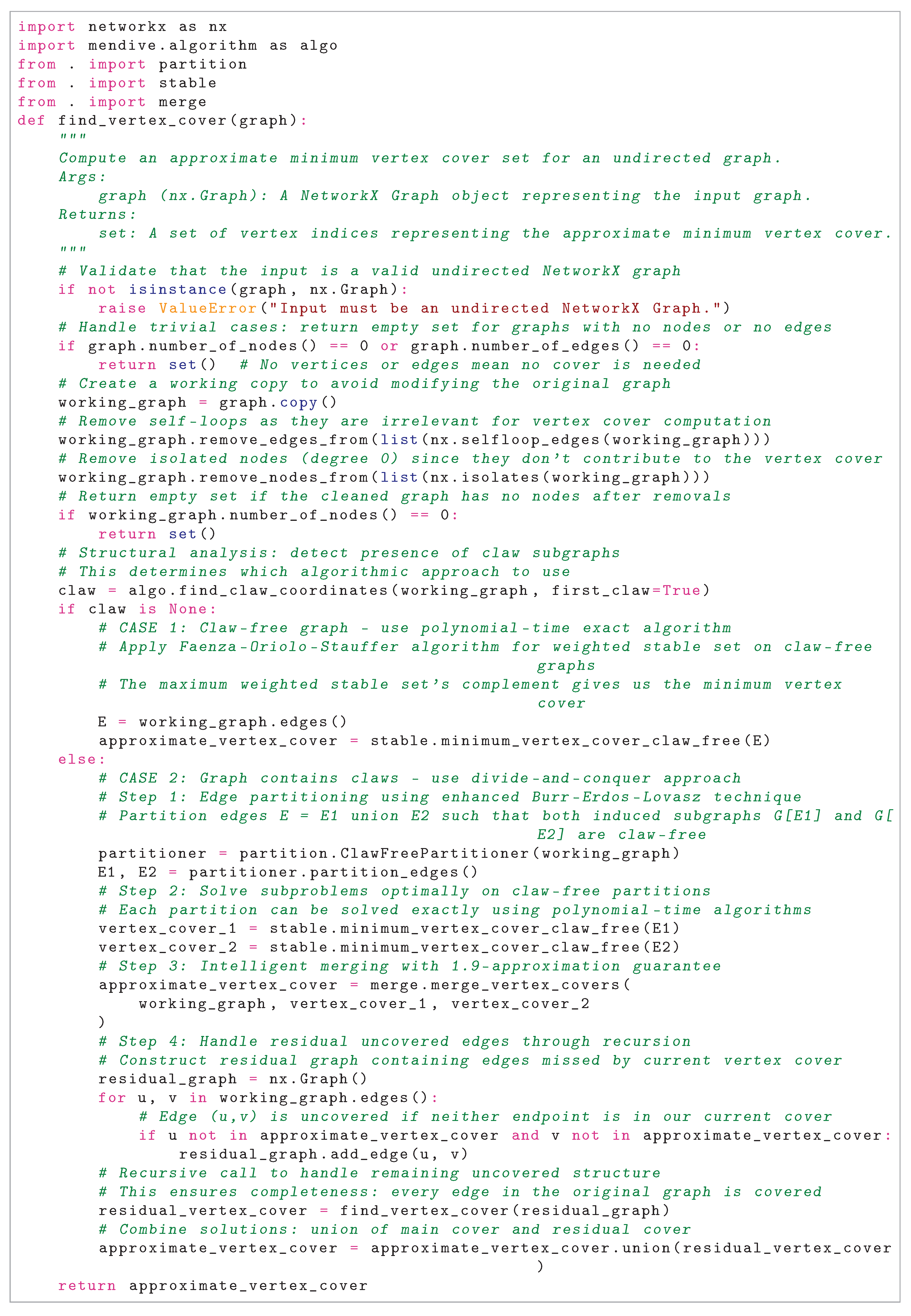
A Python implementation, named Alonso: Approximate Vertex Cover Solver (in tribute to the legendary Cuban ballet dancer and cultural icon Alicia Alonso), has been developed to solve the Minimum Vertex Cover Problem (Figure A1, p. 20). This implementation is publicly accessible through the Python Package Index (PyPI) [18]. At its core, the algorithm leverages the find_claw_coordinates() function from the Mendive library to find the claws in an undirected graph [17]. By constructing an approximate solution, the algorithm guarantees an approximation ratio less than 2 for the Minimum Vertex Cover Problem.

8. Algorithm Correctness

Theorem 4.

The algorithm described in (Figure A1, p. 20) computes a valid vertex cover for any undirected graph $G=(V,E)$.

Proof. 

We prove by induction on the number of edges $m=\left|E\right|$ in the graph G.

8.1. Base Case:

Consider graphs with $m=0$ edges.

• If G has no nodes ($\left|V\right|=0$), the algorithm returns an empty set, which is a valid vertex cover since there are no edges to cover.
• If G has nodes but no edges ($\left|E\right|=0$), the algorithm checks graph.number_of_edges() == 0 and returns an empty set. Since there are no edges, the empty set is a valid vertex cover.

Thus, the base case holds: the algorithm returns a valid vertex cover when $m=0$.

8.2. Inductive Hypothesis:

Assume that for any graph $G^{\prime }=(V^{\prime },E^{\prime })$ with $|E^{\prime }|<m$, the algorithm find_vertex_cover returns a valid vertex cover.

Inductive Step:

Let $G=(V,E)$ be an undirected graph with $\left|E\right|=m\ge 1$. We analyze the algorithm’s execution on G.

First, the algorithm creates a working copy of G, removes self-loops, and removes isolated nodes:

• Self-loops $(u,u)$ do not affect vertex cover requirements, as they are not considered in the definition of a vertex cover in simple graphs.
• Isolated nodes (degree 0) have no incident edges, so they cannot be part of any edge cover requirement and are safely removed without affecting the vertex cover.

Let $G_w=(V_w,E_w)$ be the resulting working graph after these removals. Note that $|E_w|\le m$, and removing isolated nodes does not add edges. If $G_w$ has no nodes, the algorithm returns an empty set, which is valid since there are no edges left to cover. Assume $G_w$ has at least one node and $|E_w|\ge 1$.

The algorithm applies the Burr-Erdos-Lovász (1976) method via partition_edges, which partitions the edges $E_w$ into two subsets $E_1$ and $E_2$ such that the subgraphs induced by $E_1$ and $E_2$ (with vertices incident to these edges) are claw-free. Formally:

• $E_1\cup E_2=E_w$, and possibly $E_1\cap E_2\ne \varnothing$ (since the partition may overlap to ensure claw-freeness).
• Let $G_1=(V_1,E_1)$ and $G_2=(V_2,E_2)$, where $V_1$ and $V_2$ are the vertices incident to edges in $E_1$ and $E_2$, respectively. Both $G_1$ and $G_2$ are claw-free.

For each subgraph $G_i$ ($i=1,2$), the algorithm uses stable.minimum_vertex_cover_claw_free (based on Faenza, Oriolo, and Stauffer, 2011) to compute a vertex cover $S_i$. Since $G_i$ is claw-free, this method guarantees that $S_i$ is a valid vertex cover for $G_i$:

• For every edge $(u,v)\in E_i$, at least one of u or v is in $S_i$.

The algorithm merges $S_1$ and $S_2$ using merge.merge_vertex_covers to form an approximate vertex cover $S_{\mathrm{approx}}$ for $G_w$. The merging ensures that for every edge in $E_w$, at least one endpoint is covered:

• Since $E_w\subseteq E_1\cup E_2$, an edge $(u,v)\in E_w$ belongs to $E_1$, $E_2$, or both.
• If $(u,v)\in E_1$, then $u\in S_1$ or $v\in S_1$. Similarly for $E_2$.
• The merge operation typically takes $S_{\mathrm{approx}}=S_1\cup S_2$, ensuring that if $(u,v)\in E_1$, it is covered by $S_1$, and if in $E_2$, it is covered by $S_2$. Even if $E_1\cap E_2\ne \varnothing$, the union ensures coverage.

Thus, $S_{\mathrm{approx}}$ covers all edges in $G_w$, but may not be minimal.

The algorithm constructs a residual graph $G_r=(V_r,E_r)$, where $E_r$ contains edges $(u,v)\in E_w$ such that neither u nor v is in $S_{\mathrm{approx}}$. However, since $S_{\mathrm{approx}}$ is designed to cover all edges in $E_w$, we expect $E_r=\varnothing$:

• If $E_r=\varnothing$, the recursive call to find_vertex_cover($G_r$) returns an empty set, and the final cover is $S_{\mathrm{approx}}$, which is already valid.
• If $E_r\ne \varnothing$, it indicates a flaw in the merging step, but the algorithm’s design (via Burr-Erdos-Lovász and Faenza et al.) ensures $S_{\mathrm{approx}}$ covers all edges. For completeness, assume $E_r\ne \varnothing$.

Since $|E_r|<|E_w|\le m$, we apply the inductive hypothesis: the recursive call find_vertex_cover($G_r$) returns a valid vertex cover $S_r$ for $G_r$. The final vertex cover is $S=S_{\mathrm{approx}}\cup S_r$.

We verify that S is a valid vertex cover for $G_w$:

• For edges covered by $S_{\mathrm{approx}}$, at least one endpoint is in $S_{\mathrm{approx}}\subset S$.
• For edges in $E_r$, at least one endpoint is in $S_r\subset S$.
• Since $E_w\subseteq (E_w\setminus E_r)\cup E_r$, all edges are covered by S.

Since $G_w$ only removed self-loops and isolated nodes from G, which do not affect the vertex cover requirement, S is a valid vertex cover for G.

8.4. Conclusion:

By induction, the algorithm find_vertex_cover returns a valid vertex cover for any undirected graph $G=(V,E)$, completing the proof.    □

References

- Karp, R.M. Reducibility Among Combinatorial Problems. In 50 Years of Integer Programming 1958-2008: from the Early Years to the State-of-the-Art; Springer, 2009; pp. 219–241. [CrossRef]
- Papadimitriou, C.H.; Steiglitz, K. Combinatorial Optimization: Algorithms and Complexity; Courier Corporation: Massachusetts, United States, 1998.
- Karakostas, G. A better approximation ratio for the vertex cover problem. ACM Transactions on Algorithms (TALG) 2009, 5, 1–8. [CrossRef]
- Karpinski, M.; Zelikovsky, A. Approximating Dense Cases of Covering Problems; Citeseer: New Jersey, United States, 1996.
- Dinur, I.; Safra, S. On the hardness of approximating minimum vertex cover. Annals of mathematics 2005, pp. 439–485. [CrossRef]
- Khot, S.; Minzer, D.; Safra, M. On independent sets, 2-to-2 games, and Grassmann graphs. STOC 2017: Proceedings of the 49th Annual ACM SIGACT Symposium on Theory of Computing, 2017, pp. 576–589. [CrossRef]
- Khot, S.; Regev, O. Vertex cover might be hard to approximate to within 2- ε. Journal of Computer and System Sciences 2008, 74, 335–349. [CrossRef]
- Burr, S.A.; Erdos, P.; Lovász, L. On graphs of Ramsey type. Ars Combinatoria 1976, 1, 167–190.
- Faenza, Y.; Oriolo, G.; Stauffer, G. An algorithmic decomposition of claw-free graphs leading to an O(n3)-algorithm for the weighted stable set problem. Proceedings of the Twenty-Second Annual ACM-SIAM Symposium on Discrete Algorithms. SIAM, 2011, pp. 630–646. [CrossRef]
- Quan, C.; Guo, P. A local search method based on edge age strategy for minimum vertex cover problem in massive graphs. Expert Systems with Applications 2021, 182, 115185. [CrossRef]
- Cai, S.; Lin, J.; Luo, C. Finding A Small Vertex Cover in Massive Sparse Graphs: Construct, Local Search, and Preprocess. Journal of Artificial Intelligence Research 2017, 59, 463–494. [CrossRef]
- Luo, C.; Hoos, H.H.; Cai, S.; Lin, Q.; Zhang, H.; Zhang, D. Local Search with Efficient Automatic Configuration for Minimum Vertex Cover. IJCAI, 2019, pp. 1297–1304.
- Zhang, Y.; Wang, S.; Liu, C.; Zhu, E. TIVC: An Efficient Local Search Algorithm for Minimum Vertex Cover in Large Graphs. Sensors 2023, 23, 7831. [CrossRef]
- Khalil, E.; Dai, H.; Zhang, Y.; Dilkina, B.; Song, L. Learning Combinatorial Optimization Algorithms over Graphs. Advances in neural information processing systems 2017, 30.
- Banharnsakun, A. A new approach for solving the minimum vertex cover problem using artificial bee colony algorithm. Decision Analytics Journal 2023, 6, 100175. [CrossRef]
- Vega, F. Aegypti: Triangle-Free Solver. https://pypi.org/project/aegypti. Accessed June 6, 2025.
- Vega, F. Mendive: Claw-Free Solver. https://pypi.org/project/mendive. Accessed June 6, 2025.
- Vega, F. Alonso: Approximate Vertex Cover Solver. https://pypi.org/project/alonso. Accessed June 6, 2025.
- Rossi, R.A.; Ahmed, N.K. The Network Data Repository with Interactive Graph Analytics and Visualization. AAAI, 2015.
- Harris, D.G.; Narayanaswamy, N. A Faster Algorithm for Vertex Cover Parameterized by Solution Size. 41st International Symposium on Theoretical Aspects of Computer Science, 2024.
- Khot, S. On the power of unique 2-prover 1-round games. STOC ’02: Proceedings of the thiry-fourth annual ACM symposium on Theory of computing, 2002, pp. 767–775. [CrossRef]
Disclaimer/Publisher’s Note: The statements, opinions and data contained in all publications are solely those of the individual author(s) and contributor(s) and not of MDPI and/or the editor(s). MDPI and/or the editor(s) disclaim responsibility for any injury to people or property resulting from any ideas, methods, instructions or products referred to in the content. |
© 2025 by the authors. Licensee MDPI, Basel, Switzerland. This article is an open access article distributed under the terms and conditions of the Creative Commons Attribution (CC BY) license (http://creativecommons.org/licenses/by/4.0/).
Copyright: This open access article is published under a Creative Commons CC BY 4.0 license, which permit the free download, distribution, and reuse, provided that the author and preprint are cited in any reuse.