
Submitted:
04 June 2025
Posted:
06 June 2025
You are already at the latest version
Abstract
This paper presents an alternating testing strategy to improve the reliability of multi-state Safety Instrumented Systems (SIS) under degradation conditions. A Dynamic Bayesian Network (DBN) model is developed to assess SIS unavailability, integrating proof testing parameters and capturing multi-state component behavior. Applied initially to the actuator layer of a SIS with a 1oo3 (one-out-of-three), redundancy structure, the study examines the impact of extended test durations, showing that the alternating strategy reduces non-zero test durations compared to the simultaneous test strategy. The approach is then extended to a complete SIS, with a case study demonstrating its potential to enhance system reliability and optimize maintenance management by considering degradation and redundancy factors.
Keywords:
probability failure on demand
; actuator layer
; Dynamic Bayesian Network
; hidden failures
; test strategy
; proof test duration
| Contents | ||
| 1. | Introduction. . . . . . . . . . . . . . . . . . . . . . . . . . . . . . . . . . . . . . . . . . . . . . . . . . . . . . . . . . | 2 |
| 2. | Problem Statement. . . . . . . . . . . . . . . . . . . . . . . . . . . . . . . . . . . . . . . . . . . . . . . . . . . . | 3 |
| 3. | Safety Instrumented System Structure. . . . . . . . . . . . . . . . . . . . . . . . . . . . . . . . . . . . | 3 |
| 3.1. Safety Instrumented System Structure. . . . . . . . . . . . . . . . . . . . . . . . . . . . . . | 4 | |
| 3.2. Proof Test Strategies. . . . . . . . . . . . . . . . . . . . . . . . . . . . . . . . . . . . . . . . . . . . . | 4 | |
| 4. | Materials and Methods. . . . . . . . . . . . . . . . . . . . . . . . . . . . . . . . . . . . . . . . . . . . . . . . . | 5 |
| 4.1. DBN Model. . . . . . . . . . . . . . . . . . . . . . . . . . . . . . . . . . . . . . . . . . . . . . . . . . . . . | 5 | |
| 4.2. System Unavailability Modeling. . . . . . . . . . . . . . . . . . . . . . . . . . . . . . . . . . . | 6 | |
| 4.3. Study of a 1oo3 Structure. . . . . . . . . . . . . . . . . . . . . . . . . . . . . . . . . . . . . . . . . | 8 | |
| 5. | Application. . . . . . . . . . . . . . . . . . . . . . . . . . . . . . . . . . . . . . . . . . . . . . . . . . . . . . . . . . . | 11 |
| 5.1. 1oo3 Structure. . . . . . . . . . . . . . . . . . . . . . . . . . . . . . . . . . . . . . . . . . . . . . . . . . . | 11 | |
| 5.2. Overview of the Entire SIS. . . . . . . . . . . . . . . . . . . . . . . . . . . . . . . . . . . . . . . . | 14 | |
| 5.3. Results. . . . . . . . . . . . . . . . . . . . . . . . . . . . . . . . . . . . . . . . . . . . . . . . . . . . . . . . . | 15 | |
| 6. | Conclusion. . . . . . . . . . . . . . . . . . . . . . . . . . . . . . . . . . . . . . . . . . . . . . . . . . . . . . . . . . . | 17 |
| 7. | References. . . . . . . . . . . . . . . . . . . . . . . . . . . . . . . . . . . . . . . . . . . . . . . . . . . . . . . . . . . . | 18 |
1. Introduction
Industrial facilities can present risks to people and the environment. These risks must be analyzed, assessed, and ultimately reduced to a level acceptable by society [1]. If passive risk reduction measures are insufficient to reach this level, active protection elements such as Safety Instrumented Systems (SIS) may be employed [2].
A SIS is an E/E/PE (Electrical/Electronic/Programmable Electronic) system dedicated to safety, designed to monitor the physico-chemical parameters of an Equipment Under Control (EUC), determine whether it must be placed in a safe state, and execute the necessary shutdown action. The SIS is intended to reduce risk by a given Risk Reduction Factor (RRF) to an acceptable residual level. Depending on the extent of reduction required, a specific Safety Integrity Level (SIL) must be met, which imposes both performance expectations and architectural constraints [3]. Ideally, the Safety Instrumented Function (SIF) provided by the SIS would eliminate risk completely. However, because the components of a SIS are not perfectly reliable, failures of the safety function can occur. The probability of such failures depends on the availability of the SIS components and the architecture of the system. This failure probability is measured using appropriate indicators, depending on the demand rate of the SIF [3].
When the SIS is frequently or continuously demanded (e.g., an anti-lock braking system), the performance metric is the Probability of Failure per Hour (). For low-demand applications (less than once per year, e.g., airbags), the key metric is the Average Probability of Failure on Demand (). In both cases, the SIS must execute its SIF when required. If one or more components fail or are temporarily unavailable due to maintenance or testing, the SIF may not be performed. Failures on demand often reveal latent faults or temporary unavailability of components [3].
To detect latent failures, especially in low-demand SIS, internal checks such as sensor signal comparison, partial testing, or complete proof testing of SIS components can be conducted. However, components under test are not able to perform their safety function during the test, which directly affects their instantaneous performance and, consequently, increases the PFDavg [4]. Thus, the testing strategy significantly affects performance and must be carefully evaluated [5]. This requires a flexible and accurate computational model that accounts for all relevant parameters, including those related to testing. It is equally crucial to characterize the system’s unavailability state during testing [6].
Several modeling tools are used to assess SIS performance. Fault Tree Analysis is unsuitable when partial testing is involved [7], and analytic expressions can become too complex when many parameters must be considered [8]. Markov chains are well adapted for assessing unavailability with testing, but become impractical when structural changes occur during component testing.
To address this, some authors propose switching Markov chains [9] or Stochastic Petri Nets [10,11]. However, Petri nets often require Monte Carlo simulations, which can be computationally expensive to yield accurate probability estimates. Bayesian Networks (BNs) have emerged as attractive alternatives to switching Markov models due to their modeling simplicity [12] and their ability to reflect knowledge such as known component states (e.g., under test or failed). Furthermore, Dynamic Bayesian Networks (DBNs), particularly those based on Two-Time Bayesian Networks (2TBNs), are well suited for capturing temporal variations in component reliability [13].
This article focuses on enhancing the reliability of SIS operating under degradation by proposing an alternating proof testing strategy. To support this objective, a probabilistic modeling framework based on DBNs is developed to analyze the PFDavg under various testing configurations and system degradation scenarios. The study focuses on redundant architectures and aims to :
- Investigate the influence of SIS architecture on the effectiveness of testing strategies.
- Develop a DBN model that accurately considers the behavior and dependencies of SIS components under testing conditions.
- Evaluate the impact of key test parameters (e.g., frequency, duration, coverage) on system performance through a representative case study.
To address these objectives, the paper is structured as follows: The paper is structured as follows: Section 2 discusses the problem statement, examining limitations in current approaches for modeling low-demand SIS with proof testing. In Section 3, the system architecture is defined, with emphasis on KooN structures and their implications on availability during testing. Section 4 introduces the proposed DBN modeling approach and the integration of test-related parameters. In Section 5, the proposed model is applied to a case study, evaluating testing strategies and quantifying their effects on PFDavg. Finally, Section 6 presents the main conclusions of this work outlines directions for future research.
2. Problem Statement
In Safety Instrumented Systems (SIS) operating in low-demand mode, performance is predominantly determined by three interrelated factors : the reliability of individual components, the system architecture, and the proof test strategy implemented. The average Probability of Failure on Demand (PFDavg), which serves as a key performance indicator in accordance with international safety standards such as IEC 61508 [3] and IEC 61511 [14], is directly influenced by these dimensions.
One of the critical challenges lies in the design and implementation of effective proof test strategies, which are inherently dependent on the architecture of the SIS. In simple 1oo1 configurations, which lack redundancy, testing any component renders the entire SIS temporarily unavailable. This creates a significant exposure to risk during the test period and imposes operational constraints, particularly in continuous process industries where shutdowns are costly or infeasible. In such cases, the number of testing strategies that can be effectively implemented is severely limited, as components cannot be tested independently without compromising the safety function.
The situation changes fundamentally when redundancy is introduced within the SIS layers, such as in K-out-of-N (KooN) architectures (e.g., 1oo2, 2oo3). Redundancy not only improves fault tolerance but also expands the range of applicable proof test strategies. With redundant components, it becomes possible to :
- Test components of each layer alternately, ensuring that at least one component remains operational to maintain the safety function.
- Test success paths within the redundant architecture, targeting specific combinations of components required to fulfill the safety objective.
These architectural choices open the door to alternating testing strategies, which support a more flexible and dynamic approach to maintenance and reliability management. However, optimizing such strategies requires a systematic understanding of the interdependencies among architectural redundancy, test sequencing, and component degradation behavior.
Moreover, many existing reliability models assume perfect and instantaneous testing, ignoring the realities of imperfect proof testing, non-zero test durations, and progressive degradation of components over time. These simplifications limit their applicability in real-world industrial environments, where such factors significantly affect overall system availability.
3. Safety Instrumented System Structure
To ensure safety functions, various structural approaches can be used. One straightforward method is to design a system of three distinct layers. The initial layer is tasked with monitoring the physicochemical characteristics through sensors. The logical layer processes inputs, computes decisions, and performs online diagnostics. Finally, the actuator layer executes the determined responses [15]. These layers typically adopt redundant architectures that consist of one or more components. Among the commonly utilized redundant structures are M-out-of-N (MooN) voting structures [16]. In such structures, MooN indicates that at least M out of the N components must operate correctly for the safety function to be effectively ensured.
In a standard MooN voting structure, if M equals N, it represents a serial system with N components. Conversely, if M equals 1, it signifies a parallel system with N components. This redundancy configuration is referred to as 1-out-of-N (1ooN) [16].
3.1. Safety Instrumented System Structure
Figure 1 shows the whole structure of a typical Safety Instrumented System that monitors an Entity Under Control (chemical reactor). When designing Safety Instrumented Systems, various layer structures must be considered, each incorporating redundant channels sensitive to Common Cause Failure. In Figure 1, actuators (FC) and Logic Solvers (LS) are arranged in 1oo3 voting structures. The sensor layer is separated into temperature and pressure sections, each employing a 1oo2 voting architecture.
For clarity the applicability of the proposed methodology, this study focuses on the actuator layer, modeled as a 1oo3 configuration consisting of three identical valves. These valves are designed to isolate flow and reduce excess pressure when safety limits are surpassed, ensuring the protection of the system as long as at least one valve functions as required on demand [16].
The choice of this redundant layer as the focal point allows for a detailed analysis of testing strategies, while maintaining the general applicability of the approach. Since this layer predominantly comprises mechanical components, it is particularly susceptible to degradation mechanisms and performance loss over time, making it especially suitable for reliability evaluation.
The mean value of PDF metric is used to assess a SIS operating in low-demand mode. Its assessment integrates various parameters such as failure rates, Diagnostic Coverage, and Common Cause Failure. Additionally, the testing strategy must be integrated into the unavailability assessment process. Proof testing can be conducted through various test strategies [9].
3.2. Proof Test Strategies
The primary objective of proof testing is to uncover latent dangerous failures that may not be detected by online diagnostic tests [4]. This aspect is crucial in Safety Instrumented Systems and should be integrated into performance assessments. Therefore, it’s imperative to have a comprehensive understanding of the principal parameters related to proof testing. Various proof test strategies have been defined for Safety Instrumented System verification. [17] proposed the following classification of these strategies:
- Simultaneous test: All components are tested together, necessitating a sufficient number of repair teams to test all components simultaneously. The Safety Instrumented System becomes unavailable during simultaneous testing [18].
- Sequential test: Components are tested consecutively, one after the other. Once a component is tested and restored to service, the next component is tested, assuming that other components remain operational [12].
- Staggered test: All Safety Instrumented System components are tested at different intervals. The most common form is the uniform staggered test, where each component has its own testing period, assuming the other components are functional.
- Random test: In this strategy, the test intervals for components are not predetermined but are randomly chosen [17] or computed based on the current system state.
The selection of elements or combinations thereof for testing defines the strategy. For redundant layer’s elements, choosing to test all or only one of them presents contrasting solutions, determining whether the Safety Instrumented Function remains available [16]. Additionally, proof testing effectiveness, harmlessness, and duration significantly impact performance index and modeling efforts [19]. As proof testing may not always detect all failures, its effectiveness is quantified by , representing the inability to uncover undetected failures. Parameter denotes the fraction of all detected but undetected (DU) failures during a proof test, known as the proof test coverage by some researchers [5].
Other parameters related to proof testing, such as (probability of failure due to the test) and (test duration), are crucial. corresponds to on-demand failures resulting from proof testing, while represents the test duration during which the Safety Instrumented System is reconfigured, with the tested component rendered unavailable [12].
Considering a non-null test duration and component redundancy, alternating test strategies may be used. Instead of testing the entire layer at once, a subset of components (not the full set) can be tested individually, making them temporarily unavailable while still ensuring the overall availability of the layer. However, this approach is not applicable to 1-out-of-1 (1oo1) configurations, where no redundancy exists.
Despite their significance, proof testing parameters are often overlooked in the modeling of unavailability. Therefore, the objective of this paper is to develop a model incorporating proof testing parameters and analyze their effects on unavailability.
4. Materials and Methods
4.1. DBN Model
Dynamic Bayesian Networks (DBNs) are probabilistic graphical models that capture temporal dependencies among variables by extending traditional Bayesian Networks to handle sequential and time-series data. They model system dynamics by representing the probabilistic relationships between system states across successive time steps. Fundamental to DBNs are the principles of conditional probability and Bayes’ rule, which together enable the inference of system behavior over time.
In a DBN, the conditional probability denotes the likelihood of the system being in a particular state at time k, given its state at time . This conditional distribution is governed by transition probabilities that encode how the system evolves temporally.
The general formulation of the transition model at time k is expressed as:
where represents the node at time k, and denotes the set of parent nodes of , typically including nodes from time . The term corresponds to the conditional probability of node given its parents, often encoded via Conditional Probability Tables (CPT). Equation (1) thus defines the joint distribution on all variables at time k, conditioned on their respective parents.
4.2. System Unavailability Modeling
To model the performance of a Safety Instrumented System (SIS) under varying proof testing conditions, we extend the transition model to incorporate a test state variable . Specifically, we determine, which represents the probability distribution of the state system at time k, given its state at the previous time step and the test condition . This extension allows for the representation of context-sensitive transitions, enabling the DBN to account for modifications in system behavior during proof testing phases.
DBN model thus explicitly integrates the temporal dimension of target system behavior [20]. At each discrete time step , the system state is modeled by a random variable , with its distribution determined via a CPT conditioned on . The exogenous variable , representing the activity of the proof test, serves as a selector of transition models, capturing changes in the architecture or behavior of the system. The states of the proof test are defined as follows:
- : test inactive;
- : test active;
- : test initialization phase;
- : test completion phase.
This modeling approach enables a structured and dynamic representation of SIS behavior throughout the operational and testing phases, as depicted in Figure 2.
In the proposed model, we consider a DBN defined over discrete time steps , where the system is characterized by three main variables:
- is the system state at time step k.
- : the system’s operational state at time k),
- is the possible state of the system at time k, with .
- : the test state variable at time k, where is the set of all possible test states.
- : the unavailability indicator, where is the possible unavailability state of layer, with typically indicating available or unavailable.
The evolution of the system’s state is governed by a time-inhomogeneous Markov process conditioned on the test state
The matrix denotes the conditional transition matrix under the test condition .
The gray node in Figure 2 represents the instantaneous unavailability of the system layer, modeled as a probabilistic function of the current system state and the proof test condition . It reflects the likelihood that the layer is unable to perform its safety function at time step k, considering the system’s evolving behavior and the current test phase.
is the conditional probability that the system is in unavailability state , given it is in system state and the test condition is .
The instantaneous unavailability is computed as the sum of the probabilities corresponding to the system states in which the layer failures to perform its safety function. The PFD at time step k is expressed as:
Throughout a proof test cycle of duration , where denotes the interval between two successive tests, the average unavailability is estimated using discrete-time numerical integration as follows:
4.3. Study of a 1oo3 Structure
A 1-out-of-3 (1oo3) architecture comprises three elements configured in parallel, each independently capable of performing the required safety function. This redundant structure ensures that the system remains operational and continues to provide the intended safety function as long as at least one of the three elements remains functional. This configuration enhances system reliability by tolerating up to two individual element failures without compromising overall safety [21].
In this study, an alternating test strategy is used at a fixed frequency. During testing, only one component out of three is tested while the others remain in service. Consequently, the 1oo3 structure temporarily transitions to a 1-out-of-2 (1oo2) configuration during the test and reverts to a 1oo3 structure afterward (see Figure 3). The stochastic process part in the model, represented by the relationship between and , conforms to a Markov model as illustrated in Figure 4(a).
In a system composed of three components, each of which can be in one of three states—Functional (OK), Dangerous Detected (DD), or Dangerous Undetected (DU)—a total of 27 distinct global states must initially be considered. To reduce the model’s complexity, a state grouping technique is applied, simplifying the system to 12 representative states (cf. Figure 4(b)). However, this simplification results in the loss of detailed information about the condition of individual components.
When the proposed alternating test strategy is applied with a non-zero test duration, only one component is tested at a time within the 1oo3 configuration. During testing, the selected component is temporarily removed from service, while the system remains operational if the other two components are available. As a result, the specific condition of the tested component cannot be clearly determined. To address this limitation, the system is represented by three equivalent 1oo2 configurations, each corresponding to one of the components being tested and using the same probability distribution (cf.Figure 4(b)). Each representative state in the original 1oo3 structure is interpreted differently depending on the active test scenario , as presented in Table 1.
The detailed mechanism of this transition process is presented in the following, illusrating how each state in the 1oo3 configuration is reinterpreted within the corresponding 1oo2 structures, depending on the active proof test state .
- Upon test initiation (), state probabilities before testing are redistributed across three anonymous 1oo2 structures, where one component is under test and the others are not. The corresponding CPT is outlined in Table 3.
- At the test’s conclusion (), probabilities are reallocated from three 1oo2 structures to one 1oo3 architecture, guided by the CPT presented in Table 6.
Within the framework of the proposed testing strategy, the behavior of the 1oo3 system configuration is modeled using the Dynamic Bayesian Network (DBN) depicted in Figure 2. The CPTs associated with this DBN, detailed in Table 2 through Table 6, correspond to four distinct proof test states. These CPTs reflect the different stages of the testing process and define the probabilistic transitions that influence system unavailability under various testing scenarios.
5. Application
This section presents illustrative examples to demonstrate the application of the proposed approach to evaluate the performance of a safety system. The first example focuses on simulating a 1oo3 architecture to calculate its on-demand unavailability. The second example addresses the complete Safety Instrumented System (SIS) dedicated to a chemical reactor, as initially defined by [22]. The analysis highlights key factors influencing the reliability of the system, including the role of inspection tests and the interaction between different components of the system.
5.1. 1oo3 Structure
This specific architecture, previously introduced and extensively analyzed in the preceding section, led to the formulation of several Conditional Probability Tables (CPTs), as shown in Table 2, Table 3, Table 4, Table 5 and Table 6. These CPTs represent the probabilistic dependencies between component states, conditioned on the status of the proof test, and form the core of the Dynamic Bayesian Network (DBN) model. Based on this foundation, the next step involves implementing the complete probabilistic model illustrated in Figure 2. This model enables the evaluation of system unavailability by computing the instantaneous PFD at a given time, which subsequently allows for the determination of the average PFD over the mission period (PFDavg). These two reliability indicators play a crucial role in evaluating the performance of the architecture and gaining insights into its behavior under demand scenarios.
To illustrate the applicability of the proposed model and assess the effectiveness of the testing strategy, a numerical case study is presented, focusing on a 1oo3 system architecture. Although the analysis focuses on this configuration, this choice is made strictly for illustrative purposes and does not limit the applicability of the approach to the entire SIS. Based on the defined testing strategies, two extreme cases are examined for the actuator layer operating under imperfect proof testing conditions.
- Strategy I: Simultaneous testing, where the three components are tested at the same time during each test cycle of the proof.
- Strategy II: The proposed strategy introduced in this study, where only one component is tested during each proof test interval.
A comparative analysis between the two strategies for the 1oo3 structure is presented based on proof test parameters. In our proposed model, the test nodes for each layer serve as exogenous variables, influencing the stochastic process and layer unavailability computation. By simulating the dynamic model, the instantaneous Probability of Failure on Demand for the actuator layer is computed through successive inferences using Conditional Probability Table provided in Table 3, Table 4, Table 5 and Table 6.
Under Strategy I, Figure 5(a) illustrates the variation of 1oo3 structure unavailability and its average value, , represented semi-logarithmically for two test durations (20h and 40h). Comparing the simulation cases reveals the pronounced impact of on variation. As depicted in Figure 5(a), the PFD of the structure increases to 1 for all test periods, indicating complete unavailability of the 1oo3 architecture throughout the test duration () due to simultaneous testing of all components.
To address complete unavailability, we propose modifying the test strategy for the actuator layer. Strategy II, our proposed alternating test strategy, is then implemented to mitigate the impact of prolonged test durations (). Figure 5(b) demonstrates that Strategy II induces less variation in unavailability compared to the previous case, thanks to non-simultaneous tests. The observed decrease in availability is primarily attributed to the structural change of the actuator layer from a 1oo3 to a 1oo2 configuration. Notably, the variation in due to the alternating test strategy is clearly discernible. With h, ranges from 1.0134 × (Figure 5(a)) to 0.10276 × (Figure 5(b)).
Furthermore, to assess the effectiveness of the proposed alternating proof test strategy, a detailed sensitivity analysis was carried out. This analysis explores the influence of critical parameters related to both proof and diagnostic testing on the PFDavg for the actuator layer, which is modeled using a dynamic Bayesian network (DBN) approach.
The parameters under consideration include , , , and the rate . These variables are known to play an significant role in shaping the unavailability profile of safety instrumented components. In this analysis, four distinct scenarios were investigated. In each case, two of the parameters mentioned above were varied simultaneously, while the remaining two were kept constant. This approach enables a comprehensive evaluation of the joint impact of the variable parameters on the PFDavg, and thus on the overall reliability of the system. The simulation results are illustrated using 3D surface plots, as shown in Figure 6.
The first case, illustrated in Figure 6(a), presents the variation of the PFDavg as a function of and . The results indicate that increasing either or leads to a noticeable rise in PFDavg. This shows that proof tests which are both ineffective and prone to causing failures significantly degrade system reliability. Figure 6(b) illustrates the second case, in which the influence of and on PFDavg is examined. The results demonstrate that ineffective tests allow latent faults to persist, while longer testing periods increase the exposure to unavailability. The alternating test strategy proposed in this study mitigates these effects by avoiding simultaneous testing of all redundant components, thereby preserving partial functionality during test intervals.
Figure 6(c) illustrates the third case, which investigates the combined influence of and , with and held constant. The results reveal that both parameters contribute to an increase in system unavailability, and their combined impact becomes more significant as increases. The alternating test strategy helps reduce the adverse impact of extended test durations on the PFDavg. In this final case depicted in Figure 6(d), the relationship between and is examined. PFDavg increases with higher test ineffectiveness, while it decreases with improved diagnostic coverage. This result illustrates the compensatory role of diagnostic: even if the proof test is suboptimal, a robust diagnostic system can detect failures during normal operation, significantly enhancing reliability.
The results of the sensitivity analysis emphasize the effectiveness of the proposed alternating testing strategy to reduce the negative impact of imperfect and prolonged testing on system availability. This strategy allows for alternating tests, where only one component of a layer is tested at a time, rather than testing all components simultaneously. The integration of this strategy into the maintenance planning of safety instrumented systems is therefore recommended, especially in configurations with extended proof test durations.
5.2. Overview of the Entire SIS
The considered SIS is organized into three distinct layers. The sensor layer includes two blocks, each composed of two sensors, temperature transmitters (TT) and pressure transmitters (PT), arranged in parallel. The Logic Solver (LS) layer operates in a 1oo3 configuration, whose behavior has already been described in the previous section. Finally, the actuator layer, comprising the final control elements, also follows a 1oo3 architecture.
Figure 7 illustrates the functional architecture of the SIS studied, which is organized into three distinct and independent layers. Each layer or subsystem can be individually modeled using a DBN, as depicted in the reference model of Figure 2.
The global functionality of the SIS is captured through a combination of these layer-specific models, arranged in a serial/parallel configuration. This structure enables the estimation of the overall unavailability of the system (that is, PFD), based on the unavailability of each layer, which is modeled using a configuration .
The construction of the equivalent DBN model of the entire SIS involves defining the CPTs that determine the state of each layer based on the states of its components and the status of the proof testing process. In particular, the adopted alternating test strategy assumes that, during each test cycle, only one component per layer is subjected to verification, which introduces temporal dynamics into the unavailability of the entire SIS.
The structure of each layer is represented by a dedicated node within the DBN, and the corresponding CPT can be derived with relative ease. The DBN model described in Figure 7 constitutes the equivalent probabilistic representation of the entire SIS studied. This structure is systematically derived from the functional graph depicted in Figure 2, which models the logical dependencies and dynamic interactions between the various operational layers.
The numerical data of the key parameters that characterize the components of each functional layer, together with those related to the proof testing strategies, are summarized in Table 7. These values are then used to compute the overall PFDavg of the SIS by combining the average PFDs of the individual layers, while accounting for their mutual interactions.
5.3. Results
The complete DBN was simulated over a mission time of 10,000 hours to evaluate the dynamic behavior of the SIS. Figure 8(a), Figure 8(b), Figure 8(c), and Figure 8(d) present the evolution over time of both the instantaneous PFD and the PFDavg for each operational layer of the SIS: the Sensor Layer, LS Layer, and FE Layer. The PFD curves reflect the real-time unavailability of each layer, showing repetitive oscillations due to the execution of periodic proof tests. After each test, a significant drop in PFD is observed, followed by a gradual increase caused by the accumulation of undetected failures. Superimposed on these curves, the PFDavg of each layer is plotted as a horizontal line representing the average unavailability. The global PFDavg is obtained by combining the PFDavg values of the three layers, considering the logical structure of the SIS architecture.
To further characterize the behavior of the SIS under the proposed alternating test strategy, Figure 9 presents the instantaneous evolution of the PFD for each layer, as well as for the overall SIS. The periodic oscillations visible on each curve highlight the influence of distinct testing intervals assigned to each layer: notably, the Sensor Layer, which is subject to more frequent proof tests than the LS, FE Layers, exhibits a higher density of unavailability reduction cycles.
The alternating test strategy proves effective in significantly lowering the peaks of global unavailability when compared to what would be observed under synchronized or identical testing intervals for all layers. Over time, the unavailability of each individual layer, as well as that of the complete SIS, converges toward their respective stationary PFDavg values. These results clearly demonstrate the ability of the proposed strategy to maintain system safety performance within acceptable thresholds throughout the mission duration.
6. Conclusion
This paper presents an approach to assess the performance of redundant actuator layers within Safety Instrumented Systems (SIS) under imperfect proof testing conditions. Specifically, a Dynamic Bayesian Network (DBN) model was developed to determine the instantaneous unavailability of the operational layer by integrating proof test strategies and associated parameters. Consequently, the developed framework provides a systematic and flexible methodology for constructing detailed models to evaluate SIS performance. Moreover, by explicitly considering proof test parameters, the proposed model effectively offers a dynamic representation of multi-state components during the testing phases, thus providing a better way to understand how proof tests influence system unavailability.
A numerical case study, based on a 1oo3 architecture, demonstrated that the proposed alternating test strategy can significantly improve the performance of the actuator layer, particularly when compared to the conventional simultaneous testing approach. Moreover, the analysis extended and generalized the application of this alternating test strategy to the entire SIS. As the system’s complexity increases, the number of possible states expands exponentially with the number of components, thereby highlighting the critical importance of utilizing adaptable modeling strategies.
Based on the simulation results, the proposed alternating test strategy effectively reduces the impact of extended proof test durations, which enhances the overall availability and reliability of the SIS. However, a limitation of the current approach is the assumption that only one component within a layer is tested at a time, without specifying which one. As a result, this assumption introduces potential inefficiencies, as a component may be tested multiple times during the mission, while more degraded components requiring urgent testing receive lower priority.
To address this limitation, it is possible that a more generic modeling framework could be developed, in which each component within a layer is represented by its own DBN sub-model. In this case, the alternating test strategy could then be individually applied to each component. Furthermore, by integrating maintenance policies that identify the component to be tested based on degradation states, maintenance activities could be dynamically scheduled, with priority given to the most critical components. This priority adjustment would consequently enhance the reliability and performance of complex SIS architectures, particularly under real operational conditions. Therefore, future work will focus on developing and validating such an adaptive testing and maintenance framework.
Abbreviations
The following abbreviations are used in this manuscript:
| EUC | Entity Under Control |
| CCF | Common Cause Failures |
| CRPS | Chemical Reactor Protection System |
| CPT | Conditional Probability Table |
| DBN | Dynamic Bayesian Network |
| DC | Diagnostic Coverage |
| FC | Final Control |
| IEC | International Electrotechnical Comission |
| LS | Logic Solver |
| MooN | M out of N voting system |
| MTTR | Mean Time to Repair |
| PFD | Probability of Failure on Demand |
| PFDavg | Average Probability of Faiure on Demand |
| PT | Pressure Transmitter |
| TT | Temperature Transmitter |
| SIF | Safety Instrumented Function |
| SIL | Safety Integrity Level |
| SIS | Safety Instrumented System |
References
- Aven Terje, M.Y. The strong power of standards in the safety and risk fields: A threat to proper developments of these fields? Reliability Engineering & System Safety 2019, 189, 279–286. [Google Scholar]
- Rausand, M. , Average Probability of Failure on Demand. In Reliability of Safety-Critical Systems; John Wiley & Sons, Ltd, 2014; chapter 8, pp. 191–272.
- Functional safety of Electrical/Electronic/Programmable Electronic Safety Related Systems. Part 1-7; Number IEC 61508, 2010.
- Liu, Y.; Rausand, M. Proof-testing strategies induced by dangerous detected failures of safety-instrumented systems. Reliability Engineering & System Safety 2016, 145, 366–372. [Google Scholar]
- Jin, J.; Pang, L.; Hu, B.; Wang, X. Impact of proof test interval and coverage on probability of failure of safety instrumented function. Annals of Nuclear Energy 2016, 87, 537–540. [Google Scholar] [CrossRef]
- Rabah, B.; Younes, R.; Djeddi, C.; Laouar, L. Optimization of safety instrumented system performance and maintenance costs in Algerian oil and gas facilities. Process Safety and Environmental Protection 2024, 182, 371–386. [Google Scholar] [CrossRef]
- Belland, J.; Wiseman, D. Using fault trees to analyze safety-instrumented systems. In Proceedings of the 2016 Annual Reliability and Maintainability Symposium (RAMS); 2016; pp. 1–6. [Google Scholar]
- Rausand, M.; Hoyland, A. System Reliability Theory; Models, Statistical Methods and Applications., 2nd ed.; New York, Wiley, 2004.
- Mechri, W.; Simon, C.; Ben Othman, K. Switching Markov chains for a holistic modeling of SIS unavailability. Reliability Engineering & System Safety 2015, 133, 212–222. [Google Scholar]
- Signoret, J.P.; Dutuit, Y.; Cacheux, P.J.; Folleau, C.; phane Collas, S.; Thomas, P. Make your Petri nets understandable: Reliability block diagrams driven Petri nets. Reliability Engineering and Safety System 2013, 113, 61–75. [Google Scholar] [CrossRef]
- Wang, C.; Gou, J.; Tian, Y.; Jin, H.; Yu, C.; Liu, Y.; Ma, J.; Xia, Y. Reliability and availability evaluation of subsea high integrity pressure protection system using stochastic Petri net. Proceedings of the Institution of Mechanical Engineers, Part O: Journal of Risk and Reliability 2022, 236, 508–521. [Google Scholar] [CrossRef]
- Simon, C.; Mechri, W.; Capizzi, G. Assessment of Safety Integrity Level by simulation of Dynamic Bayesian Networks considering test duration. Journal of Loss Prevention in the Process Industries 2019, 57, 101–113. [Google Scholar] [CrossRef]
- Weber, P.; Simon, C. Benefits of Bayesian networks Models; ISTE-Wiley, 2016.
- Functional Safety - Safety instrumented systems for the process industry sector; Number IEC 61511, 2000.
- Mechri, W. Evaluation de la Performance des Systèmes Instrumentés de Sécurité à Paramètres Imprécis. Theses, University of Tunis El-Manar, Tunisie., 2011.
- Zhang, A.; Wu, S.; Fan, D.; Xie, M.; Cai, B.; Liu, Y. Adaptive testing policy for multi-state systems with application to the degrading final elements in safety-instrumented systems. Reliability Engineering & System Safety 2022, 221, 108360. [Google Scholar]
- Torres-Echeverria, A.; Martorell, S.; Thompson, H. Multi-objective optimization of design and testing of safety instrumented systems with MooN voting architectures using a genetic algorithm. Reliability Engineering & System Safety 2012, 106, 45–60. [Google Scholar]
- Mechri, W.; Simon, C.; Bicking, F.; Ben Othman, K. Probability of failure on demand of safety systems by Multiphase Markov Chains. In Proceedings of the Conference on Control and Fault-Tolerant Systems (SysTol); 2013; pp. 98–103. [Google Scholar]
- Mechri, W.; Simon, C.; Rajhi, W. Alternating Test Strategy for Multi-State Safety System Performance Analysis. In Proceedings of the 2023 9th International Conference on Control, Decision and Information Technologies (CoDIT); 2023; pp. 914–919. [Google Scholar]
- Weber, P.; Jouffe, L. Complex system reliability modelling with Dynamic Object Oriented Bayesian Networks (DOOBN). Reliability Engineering and System Safety 2006, 91, 149–162. [Google Scholar] [CrossRef]
- Innal, F.; Lundteigen, M.A.; Liu, Y.; Barros, A. PFDavg generalized formulas for SIS subject to partial and full periodic tests based on multi-phase Markov models. Reliability Engineering & System Safety 2016, 150, 160–170. [Google Scholar]
- Torres-Echeverria, A.; Martorell, S.; Thompson, H. Modelling and optimization of proof testing policies for safety instrumented systems. Reliability Engineering and System Safety 2009, 94, 838–854. [Google Scholar] [CrossRef]
Figure 1.
Example of a typical Safety Instrumented System
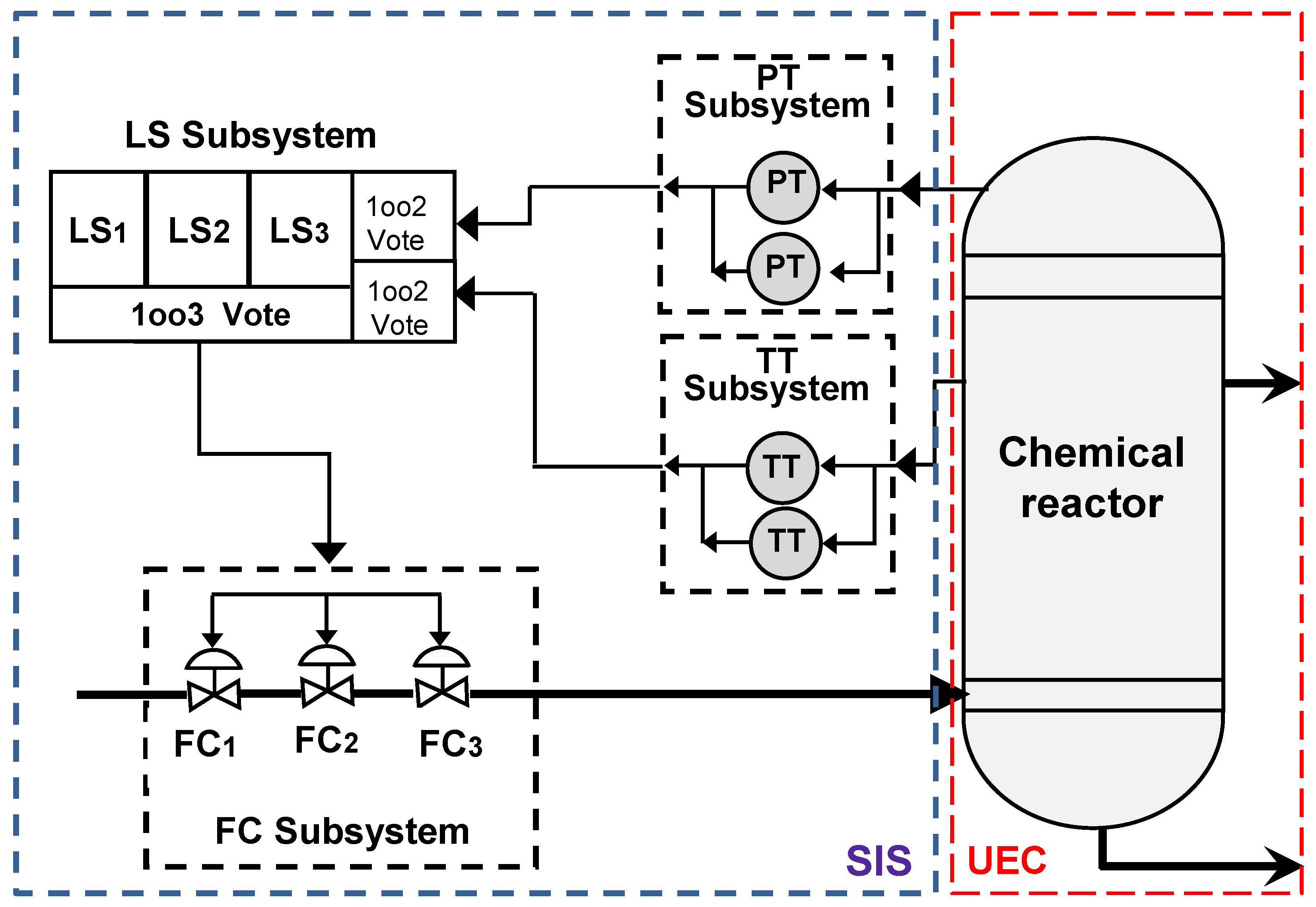
Figure 2.
DBN for unavailability modeling
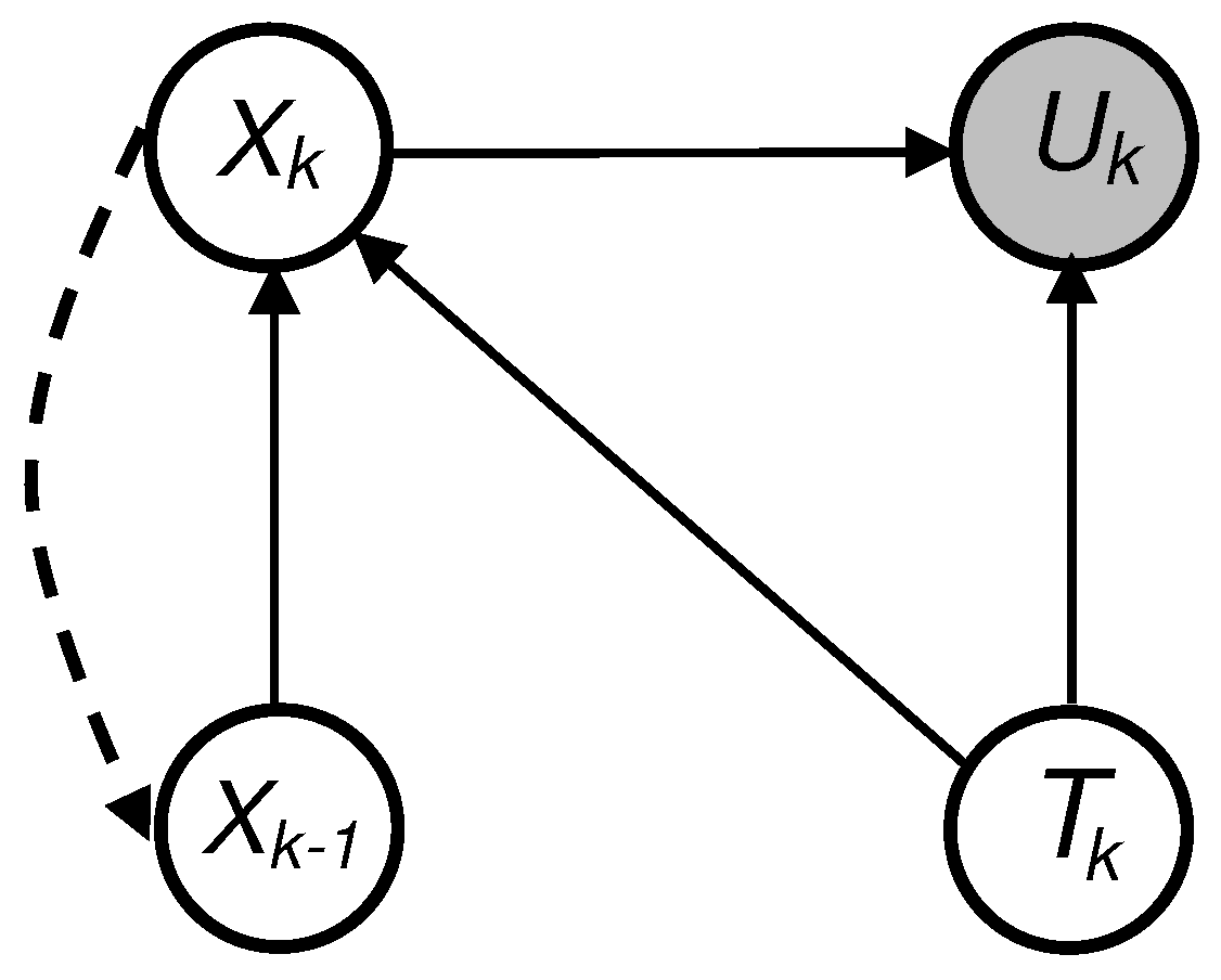
Figure 3.
Cycle of model structures from 1oo3 to 1oo2
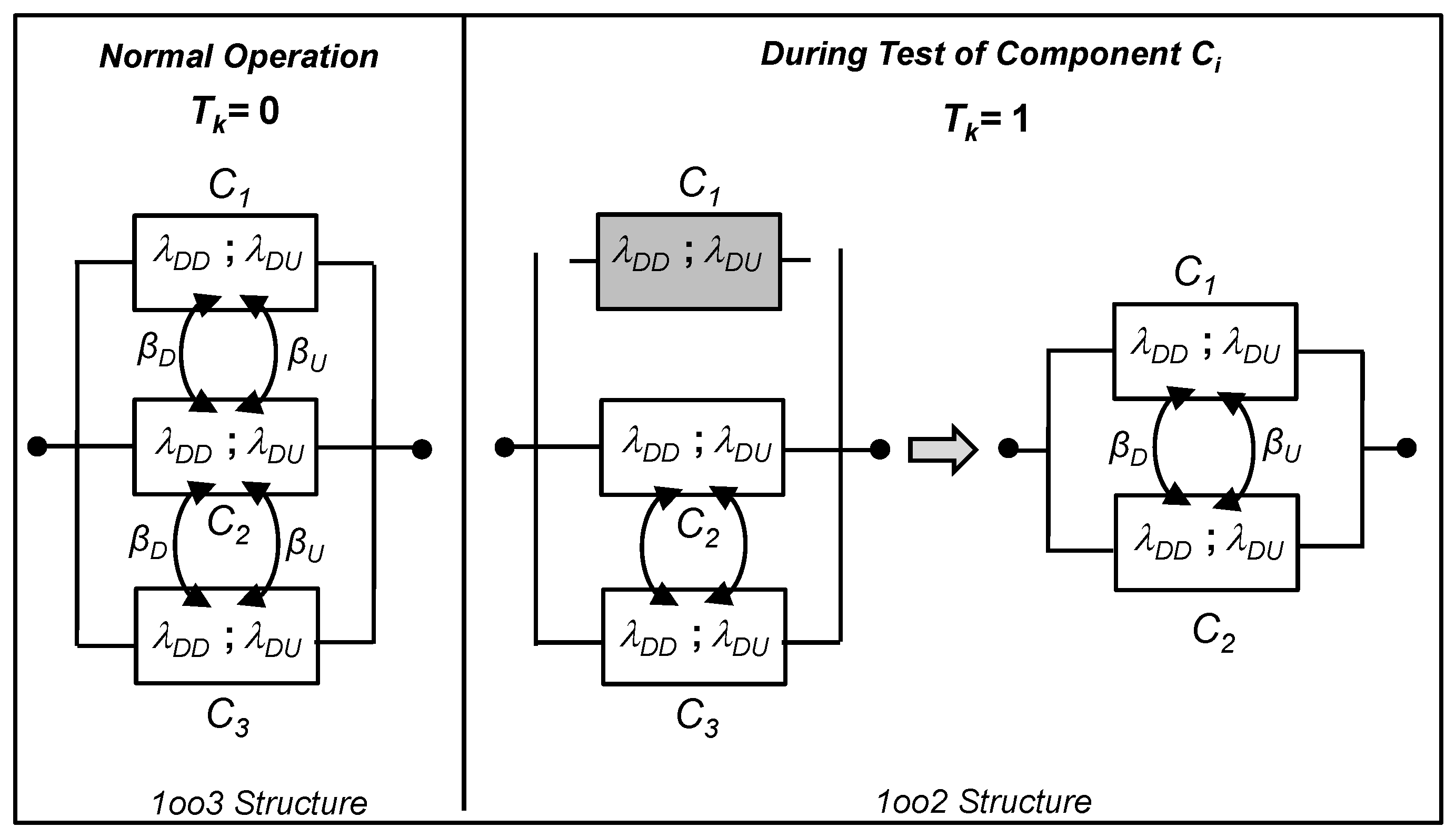
Figure 4.
Markov chains of 1oo3 layer given the test
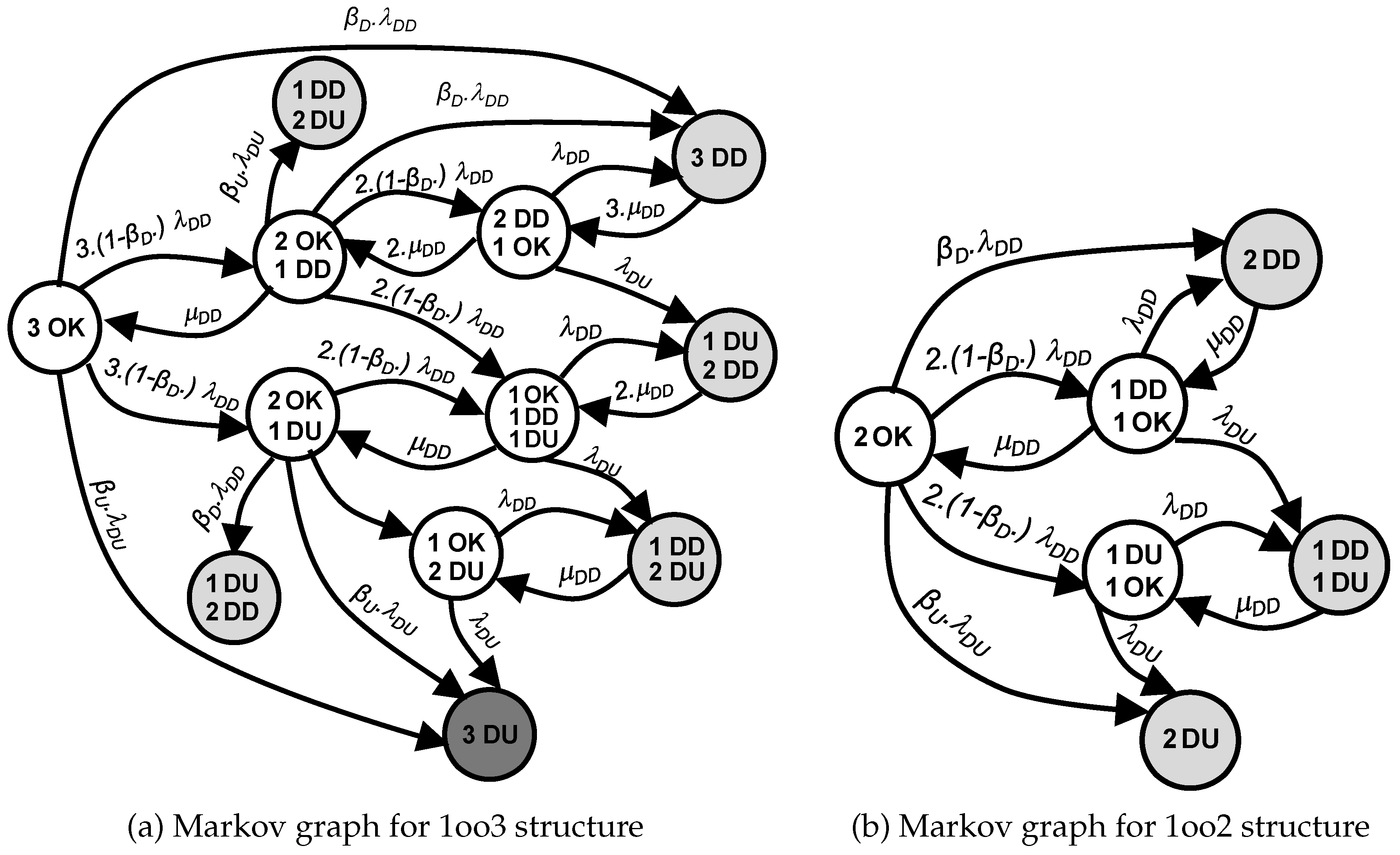
Figure 5.
PFD and PFDavg of 1oo3 structure
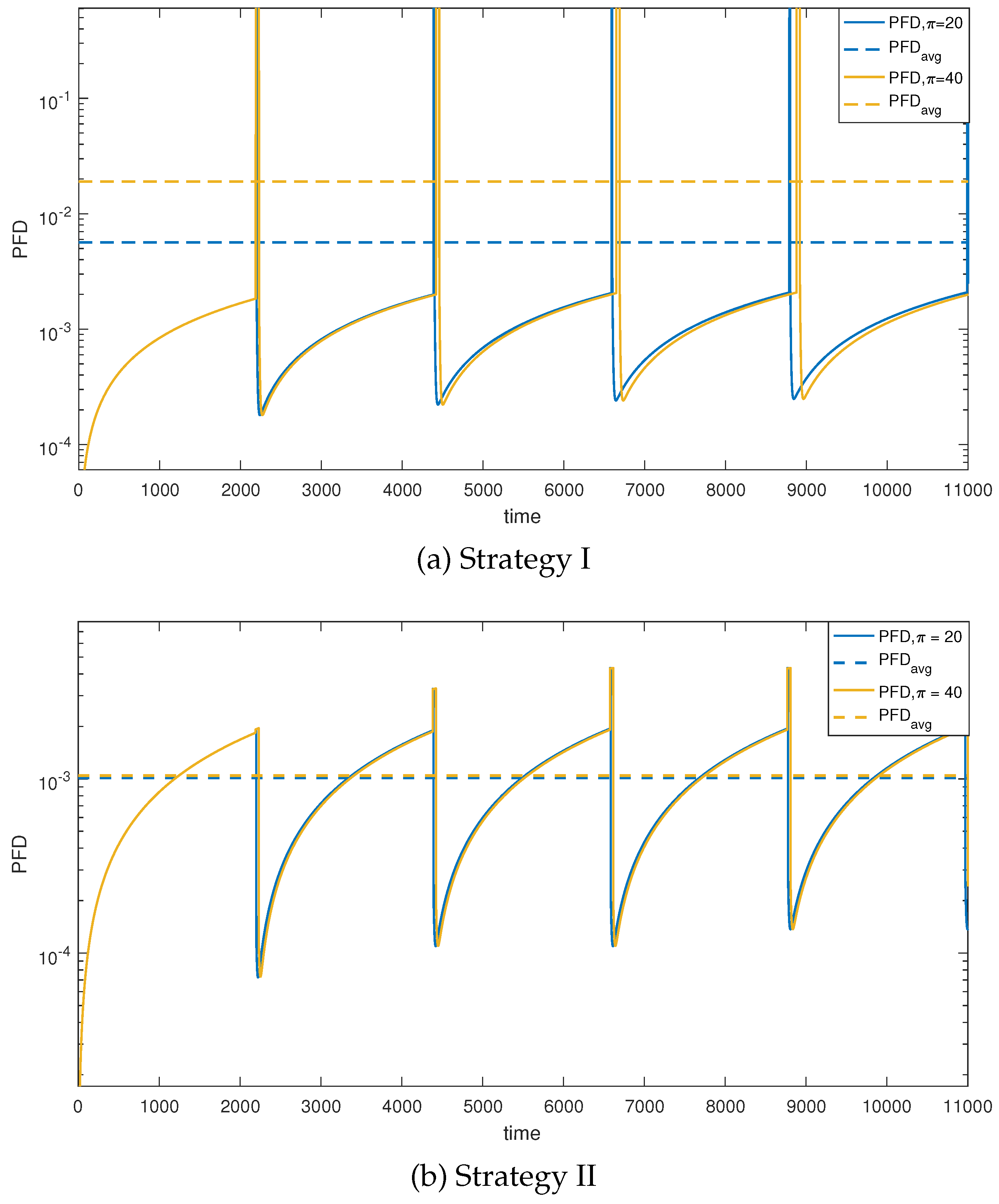
Figure 6.
PFDavg variation of 1oo3 structure according to proof test parameters
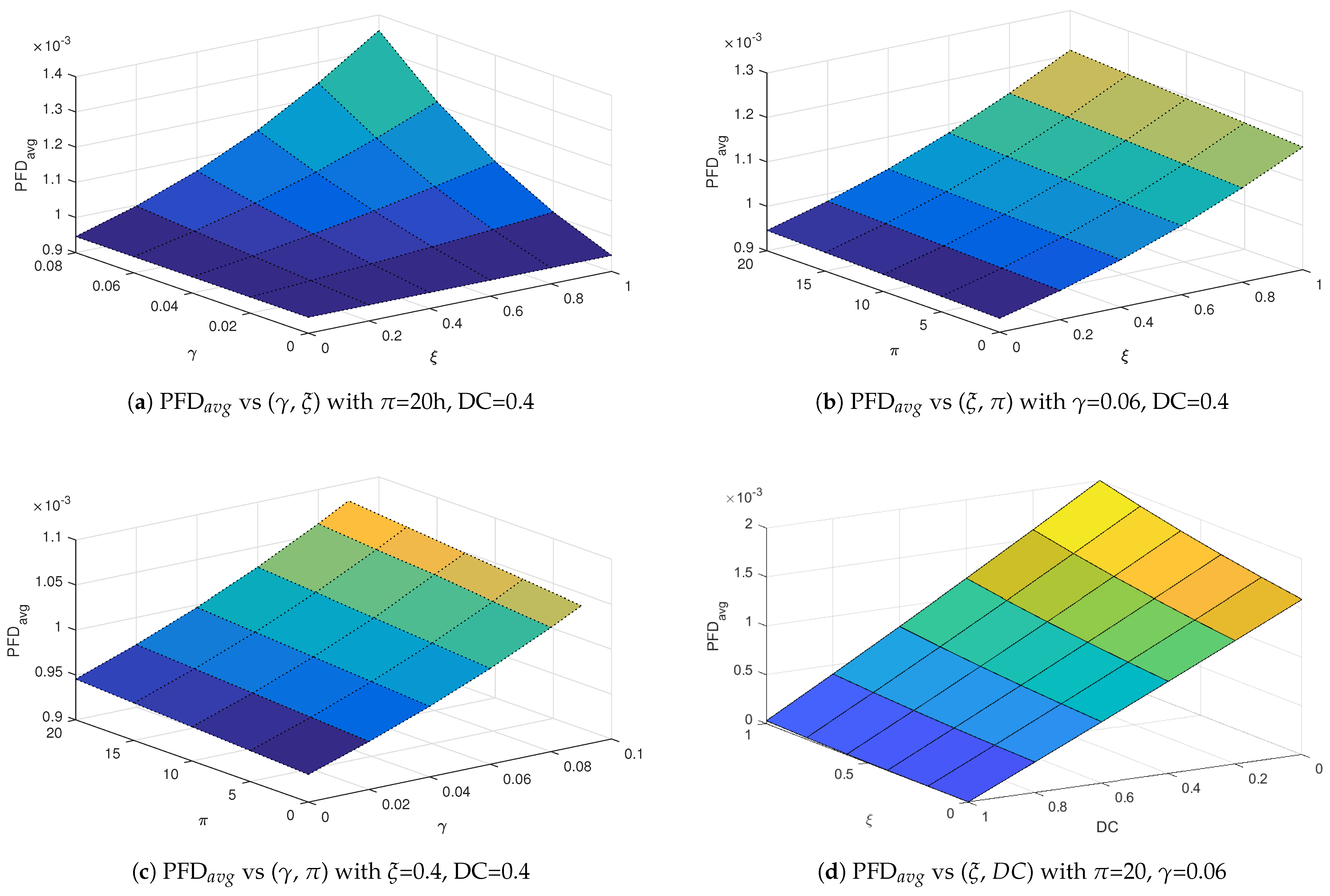
Figure 7.
DBN model of the Entire SIS
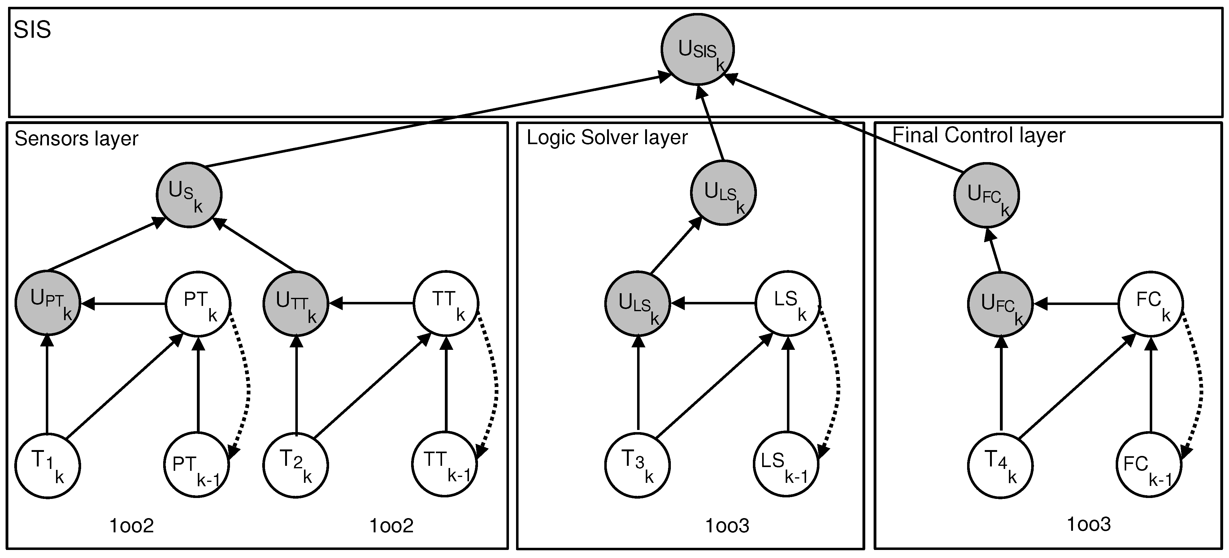
Figure 8.
Variation of PFD and PFDavg for the Overall SIS and Individual Layers
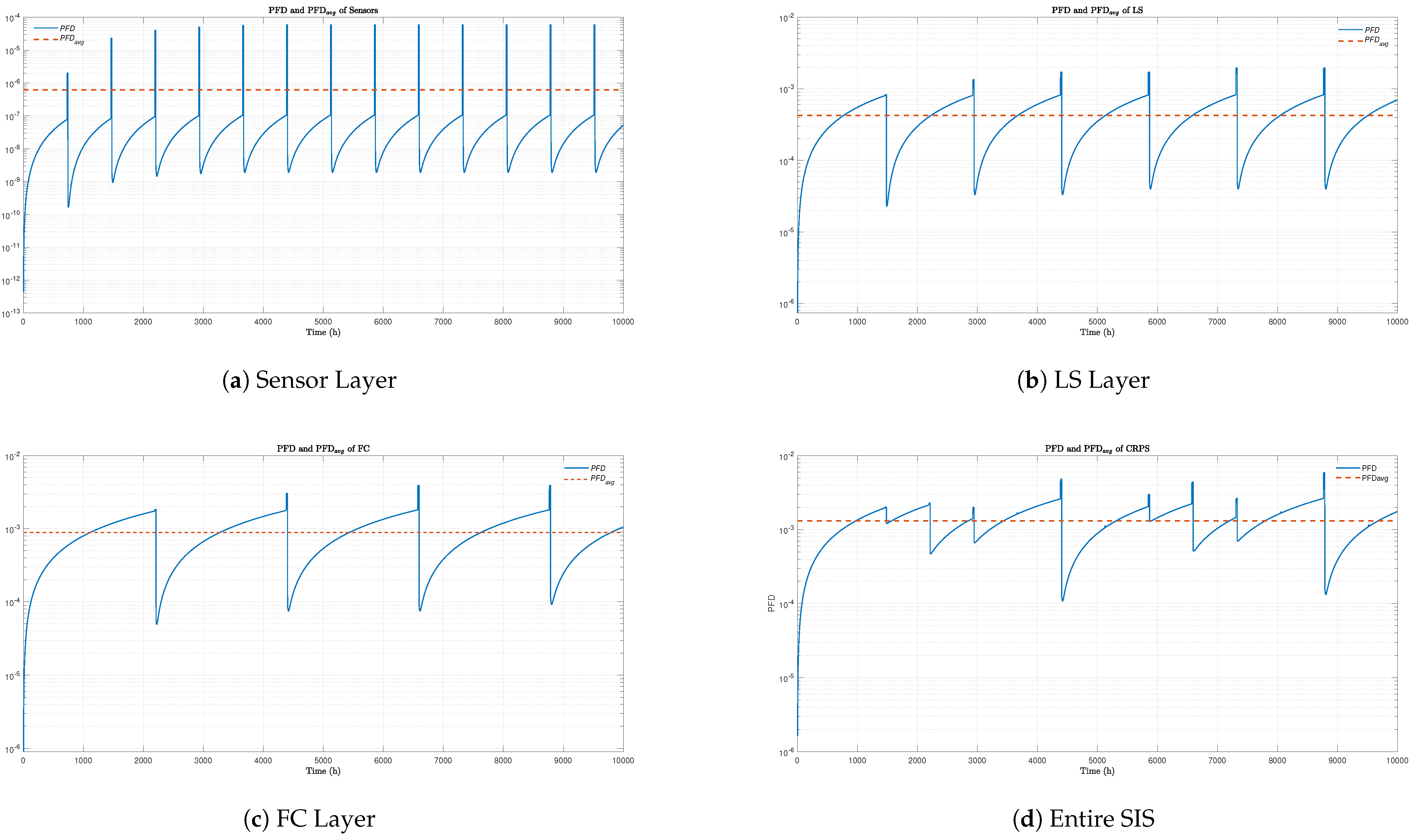
Figure 9.
Variation of PFD and PFDavg for the Overall SIS
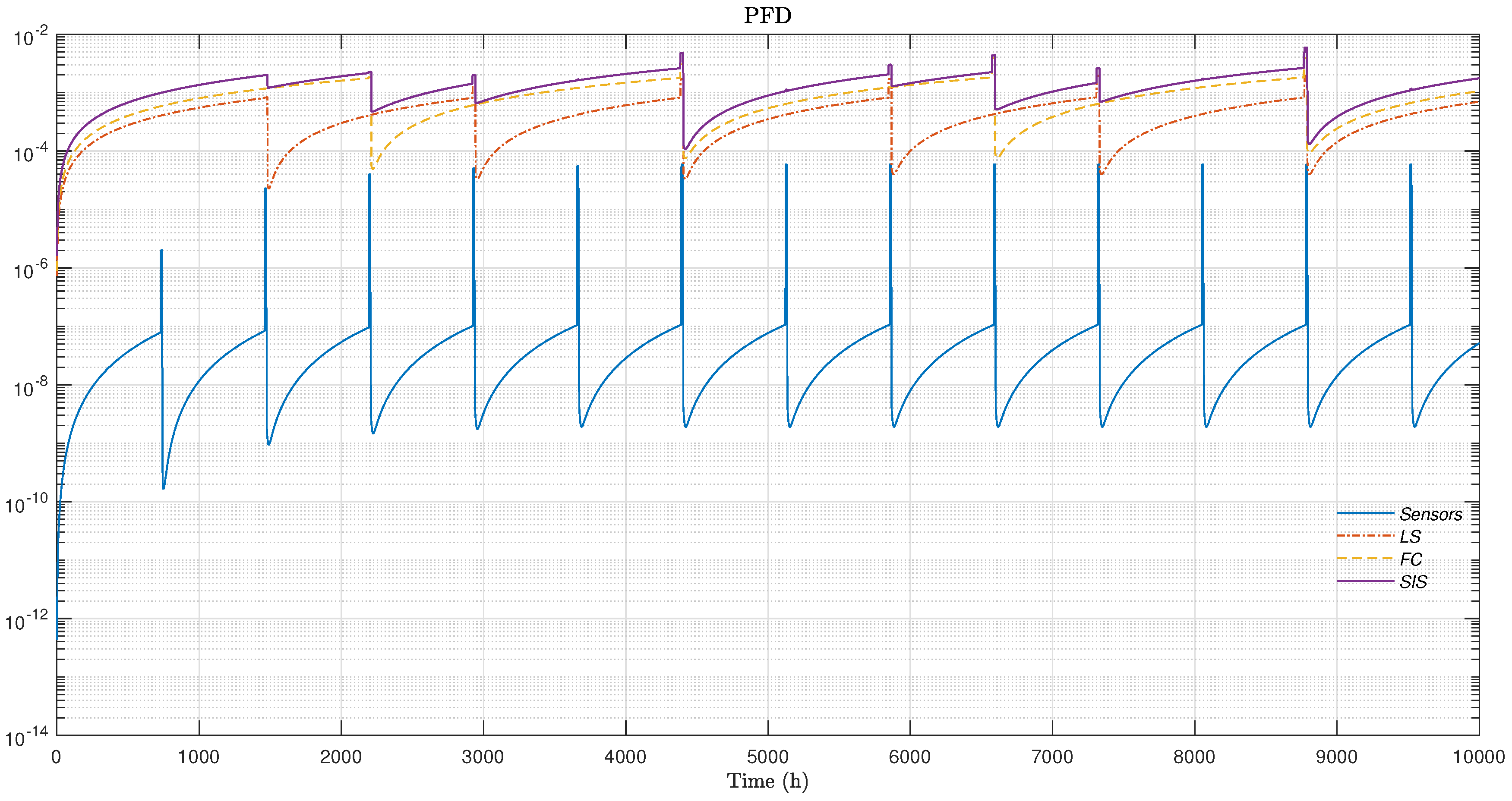

Table 1.
States of a 1oo3 structure given test phase
| States | Test phases | |
|---|---|---|
| () | () | |
| () | () | |
| {3OK} | {2OK} | |
| {2OK, 1DD} | {1OK, 1DD} | |
| {2OK, 1DU} | {1OK, 1DU} | |
| {1OK, 2DD} | {2DD} | |
| {1OK, 1DD, 1DU} | {1DD, 1DD} | |
| {1OK 2DU} | {2DU} | |
| {3DD} | {2OK} | |
| {2DD, 1DU} | {1OK, 1DD} | |
| {1DD, 2DU} | {1OK, 1DU} | |
| {3DU} | {2DD} | |
| - | {1DD, 1DD} | |
| - | {2DU} | |
| - | {2OK} | |
| - | {1OK, 1DD} | |
| - | {1OK,1DU} | |
| - | {2DD} | |
| - | {1DD, 1DU} | |
| - | {2DU} | |
Table 2.
CPT of 1oo3 system when ()
| {3OK} | {2OK,1DD} | {2OK,1DU} | {1OK,2DD} | {1OK,1DD,1DU} | {1OK,2DU} | {3DD} | {2DD,1DU} | {1DD,2DU} | {3DU} | ||
| {3OK} | - | 0 | 0 | 0 | 0 | 0 | |||||
| {2OK,1DD} | - | 0 | 0 | 0 | 0 | ||||||
| {2OK,1DU} | 0 | 0 | - | 0 | 0 | 0 | |||||
| {1OK,2DD} | 0 | 0 | 0 | - | 0 | 0 | 0 | 0 | |||
| {1OK,1DD,1DU} | 0 | 0 | 0 | 0 | - | 0 | 0 | 0 | |||
| 0 | {1OK,2DU} | 0 | 0 | 0 | 0 | 0 | - | 0 | 0 | ||
| {3DD} | 0 | 0 | 0 | 0 | 0 | - | 0 | 0 | 0 | ||
| {2DD,1DU} | 0 | 0 | 0 | 0 | 0 | 0 | - | 0 | 0 | ||
| {1DD,2DU} | 0 | 0 | 0 | 0 | 0 | 0 | 0 | - | 0 | ||
| {3DU} | 0 | 0 | 0 | 0 | 0 | 0 | 0 | 0 | 0 | 1 | |
Table 3.
CPT of 1oo3 system when ()
| {2OK} | {1OK,1DD} | {1OK,1DU} | {2DD} | {1DD,1DU} | {2DU} | |
| {3OK} | 1/3 | 0 | 0 | 0 | 0 | 0 |
| {2OK,1DD} | 1/6 | 1/6 | 0 | 0 | 0 | 0 |
| {2OK,1DU} | 1/6 | 0 | 1/6 | 0 | 0 | 0 |
| {1OK,2DD} | 0 | 1/6 | 0 | 1/6 | 0 | 0 |
| {1OK,1DD,1DU} | 0 | 1/9 | 1/9 | 0 | 1/9 | 0 |
| {1OK, 2DU} | 0 | 0 | 1/6 | 0 | 0 | 1/6 |
| {3DD} | 0 | 0 | 0 | 1/3 | 0 | 0 |
| {2DD,1DU} | 0 | 0 | 0 | 1/6 | 1/6 | 0 |
| {1DD,2DU} | 0 | 0 | 0 | 0 | 1/6 | 1/6 |
| {3DU} | 0 | 0 | 0 | 0 | 0 | 1/3 |
Table 4.
CPT of 1oo3 structure when ()
| … | … | … | |||||||
| - | – | - | 0 | … | 0 | 0 | … | 0 | |
| ⋮ | - | 1oo2 | - | ⋮ | ⋱ | ⋮ | ⋮ | ⋱ | ⋮ |
| - | – | - | 0 | … | 0 | 0 | … | 0 | |
| 0 | … | 0 | - | – | - | 0 | … | 0 | |
| ⋮ | ⋮ | ⋱ | 0 | - | 1oo2 | - | ⋮ | ⋱ | ⋮ |
| 0 | … | 0 | - | - | - | 0 | … | 0 | |
| 0 | … | 0 | 0 | … | 0 | - | – | - | |
| ⋮ | ⋮ | ⋱ | ⋮ | ⋮ | ⋱ | ⋮ | - | 1oo2 | - |
| 0 | … | 0 | 0 | … | 0 | - | – | - | |
Table 5.
CPT of 1oo2 structure
| {2OK} | {1OK,1DD} | {1OK,1DU} | {2DD} | {1DD,1DU} | {2DU} | ||
| {2OK} | - | 0 | |||||
| {1OK,1DD} | - | 0 | 0 | ||||
| {1OK,1DU} | 0 | 0 | - | 0 | |||
| 0 | {2DD} | 0 | 0 | - | 0 | 0 | |
| {1DD,1DU} | 0 | 0 | 0 | - | 0 | ||
| {2DU} | 0 | 0 | 0 | 0 | 0 | 1 | |
Table 6.
CPT of 1oo3 structure when )
| 0 | 0 | 0 | 0 | 0 | 0 | 0 | ||||
| 0 | 0 | 0 | 0 | 0 | 0 | 0 | ||||
| 0 | 0 | 0 | 0 | 0 | 0 | 0 | ||||
| 0 | 0 | 0 | 0 | 0 | 0 | 0 | ||||
| 0 | 0 | 0 | 0 | 0 | 0 | 0 | ||||
| 0 | 0 | 0 | 0 | 0 | 0 | 0 | ||||
Table 7.
Numerical data parameters of components
| Components | PTi | TTi | LSi | FCi | |
|---|---|---|---|---|---|
| Parameters | |||||
| 5.00 | 5.00 | 1.15 | 4.15 | ||
| 0.4 | 0.4 | 0.65 | 0.5 | ||
| 20 | 20 | 20 | |||
| MTTR (h) | 8 | 8 | 10 | 8 | |
| 730 | 730 | 1460 | 2190 | ||
| 0.5 | 0.5 | 0.35 | 0.45 | ||
| 0.002 | 0.002 | 0.001 | 0.007 | ||
Disclaimer/Publisher’s Note: The statements, opinions and data contained in all publications are solely those of the individual author(s) and contributor(s) and not of MDPI and/or the editor(s). MDPI and/or the editor(s) disclaim responsibility for any injury to people or property resulting from any ideas, methods, instructions or products referred to in the content. |
© 2025 by the authors. Licensee MDPI, Basel, Switzerland. This article is an open access article distributed under the terms and conditions of the Creative Commons Attribution (CC BY) license (http://creativecommons.org/licenses/by/4.0/).
Copyright: This open access article is published under a Creative Commons CC BY 4.0 license, which permit the free download, distribution, and reuse, provided that the author and preprint are cited in any reuse.


