
Submitted:
28 October 2025
Posted:
29 October 2025
You are already at the latest version
Abstract
Equipment failure is the leading cause of industrial operational disruption. Unplanned downtime equipment accounts for 11% of manufacturing revenue, highlighting the need for effective proactive maintenance strategies, such as protective sensors that can detect potential failures in critical equipment before a functional failure occurs. However, sensors are also subject to hidden failures, requiring periodic inspections to ensure proper functioning. This study proposes a novel, integrated, and generic multimethodological approach combining discrete event simulation, Monte Carlo, optimization, risk analysis, and multicriteria decision analysis methods to determine the optimal inspection period for a protective sensor subject to hidden failures. Alternative inspection periods are evaluated based on their risk-informed overall values, considering multiple conflicting Key Performance Indicators, such as maintenance costs and equipment availability. The optimal inspection period is then selected considering uncertainties and the intertemporal, intra-criterion, and inter-criteria preferences of the organization. The effectiveness of the approach is demonstrated through a case study applied at the leading Portuguese electric utility, replacing previous empirical inspection standards that did not consider economic costs and uncertainties, supported by an open, transparent, auditable, and user-friendly decision support system implemented in Microsoft Excel using only built-in functions and modeled based on the principles of Probability Management.
Keywords:
sensors
; inspection period
; maintenance
; optimization-simulation
; multicriteria
; risk
; probability management
1. Introduction
Unplanned downtime costs are estimated at 11% of revenue in the world’s 500 largest manufacturing companies and continue to increase [1]. Unplanned, reactive, or run-to-failure corrective maintenance is no longer viable for managing critical equipment. Instead, systematic preventive maintenance, after a pre-specified operating period, has become the norm. However, in environments where functional failures can lead to severe consequences, these maintenance policies have been superseded by proactive failure management strategies, such as on-condition, predictive, condition-based, or condition-monitoring maintenance tasks, which can detect a potential failure before it degrades into a functional failure [2].
Protective sensors are often used to continuously gather real-time data on equipment conditions, indicating that a functional failure is imminent or occurring. These continuous (online) monitoring sensors can detect a potential failure in critical equipment before it escalates, enabling timely maintenance decisions that prevent functional failures from occurring, which would result in longer and more costly downtimes. For instance, it is often possible to take advantage of the degradation of an equipment’s condition to infer that it has started its failure development period (a.k.a. P-F interval), that is, the time interval until a functional failure occurs [2]. Prompt action can then be taken, either manually or automatically (e.g., via an actuator), to shut down the critical equipment, repair it, and mitigate more severe consequences that could result from a functional failure.
However, protective sensors are not immune to failures. Therefore, it is essential to guarantee that the sensor is functioning properly while conducting its protective function for the critical equipment. Even though sensor failures might be evident and detected immediately, they often remain hidden (a.k.a. silent, pending, unrevealed, latent, or not self-announcing) and unnoticed until they manifest themselves through breakdowns or more serious consequences in the protected equipment, leading to significant equipment reactivation costs and long recovery downtimes [3]. Hidden failures can account for up to half of the failure modes [2,3].
In this two-unit sensor-equipment system, two scenarios can arise when the equipment fails:
- The monitoring sensor is well-functioning, detecting, and issuing an early warning of a potential failure in the protected critical equipment in a timely manner, allowing for a prompt equipment shutdown and repair, with minor equipment repair costs and downtime;
- The monitoring sensor is either ineffective (due to a hidden failure) or non-operational (because it has failed and is still under repair) and a multiple failure occurs in the system, leading to significant consequences in terms of equipment reactivation costs and downtime.
To reduce the probability that the protective sensor is not effectively monitoring and protecting the critical equipment, the former must be inspected periodically to check for the presence of hidden failures [4]. Inspection intervals (a.k.a. failure finding intervals) may be either constant (periodic) or different (sequential or non-periodic). The common practice in the industry is to implement a calendar-based inspection policy with periodic and scheduled inspections, at fixed and equal intervals calendar intervals due to its applicability and feasibility [5].
Naturally, periodic (off-line) sensor inspections incur their own costs and other consequences. Hence, the trade-off between the consequences of failure-finding inspections in the protective sensor and the consequences of a functional failure in the equipment must be assessed. It is expected that less frequent sensor inspections (and hence longer inspection periods) will decrease the probability of detecting a failure in the equipment and consequently:
- On the one hand, the expected sensor inspection costs and equipment availability will decrease;
- On the other hand, the expected equipment reactivation costs and downtime are likely to increase.
Therefore, an optimal interval between periodic inspections is expected to exist, corresponding to the best compromise between the multiple conflicting organizational Key Performance Indicators (KPIs) (e.g., minimizing total maintenance costs, and maximizing equipment availability) regarding the equipment’s functioning. This compromise can be solved by eliciting the specific preferences of the organization regarding those trade-offs, that is, how much it is willing to lose in one KPI (e.g., total costs) to gain in another (e.g., equipment availability).
Therefore, the main purpose of this article is to present an integrated risk-informed multicriteria value optimization-simulation approach to determine the optimal inspection period for a protective sensor, subject to hidden failures, monitoring the condition of a critical system. This aim is proposed to be achieved by addressing the following research questions:
- How to represent and model uncertainties in the occurrence of failures in the equipment and sensor?
- How to predict the consequences of the occurrence of system failures on multiple KPIs, such as total maintenance costs and equipment availability, considering distinct sensor inspection periods, costs, times, and other parameters of the system and the organization?
- How to model and compare the value and risk of distinct sensor inspection periods, considering their uncertainty and consequences on multiple conflicting organizational KPIs?
- How to find the optimal inspection period considering the previous issues in an integrated and robust approach?
- How to develop a decision support system that can be easily understood, audited, and used in practice by the organization?
The specific objectives of this article are to answer these research questions through an integrated and generic multimethodological approach and to demonstrate its effectiveness through its application to a real-world case study supported by an open, transparent, auditable, and user-friendly decision support system (DSS).
The remainder of this paper is organized as follows. The next section presents a description of the specific proactive maintenance problem tackled by the article, highlighting its multicriteria and stochastic nature, introducing the most important challenges that underpin its analysis and resolution, including a short review of the state of the art on similar published approaches to tackle the research problem of this article, and building the case for the need and contribution of the methodological framework presented in this article. Section 3 describes the proposed methodology. It starts with a formal definition of the problem, presenting the assumptions and building blocks of the methodology, and detailing the methods, variables, parameters, and equations used in each step of the framework. Section 4 illustrates the application of the approach through a case study supported by a DSS. Section 5 discusses the article’s main contributions to the research literature and practice and identifies its strengths and limitations. Section 6 concludes the paper and suggests potential avenues for future research.
2. State of the Art and Research Gap
Industrial systems degrade over time, leading to system failures that result in increased costs, unexpected machine unavailability, and quality and safety issues. While maintenance has historically been regarded as a reactive necessity, it is now recognized as a critical activity of asset management aimed at improving organizational efficiency, reliability, and profitability [6].
Within the context of Industry 4.0 and 5.0, traditional maintenance approaches - such as reactive and preventive maintenance - are progressively being replaced by more proactive strategies based on condition monitoring and predictive analytics, which aim to reduce maintenance costs and improve equipment availability and reliability [7,8].
A proactive maintenance system typically comprises two main types of components: (i) critical entities that perform the system’s fundamental function, and (ii) auxiliary entities that provide information, redundancy, and/or protection [9,10]. Protective components serve to mitigate the consequences of the protected critical equipment failure, which would otherwise be significantly more severe [2].
Proactive maintenance relies heavily on sensor data to monitor equipment condition, enabling early anomaly detection, performance optimization, increased system reliability, and the dynamic scheduling of maintenance interventions before failures occur. Predictive maintenance combines historical sensor data with predictive models based on statistical, forecasting, or artificial intelligence methods to estimate the likelihood and timing of future failures [11,12,13,14].
Reliability Centered Maintenance (RCM) constitutes a structured and widely adopted proactive framework that prioritizes critical assets and enables the development of customized maintenance plans, which reduce downtime and operational disruptions, extend equipment lifespan, and promote more efficient, reliable, sustainable, and cost-effective operations, ultimately improving product quality and customer satisfaction. RCM plans track equipment performance through a combination of condition-based monitoring of real-time sensor data and predictive analytics to anticipate failures and schedule preventive maintenance interventions accordingly before failures escalate into major consequences [3,15].
Nevertheless, most maintenance decision studies assume that the monitoring sensor is perfect, that is, its information signal is accurate to the actual state of the equipment, overlooking the compounded effect of sensor unreliability due to the presence of hidden failures. Faulty sensors that produce erroneous signals lead to incorrect maintenance decisions [16]. Research on the maintenance of a critical system with an unreliable protective system is limited [17]. Hence, more research should be conducted to study the effects of imperfect condition monitoring on optimal dynamic maintenance decisions, namely, new models and methodologies that determine the optimal inspection maintenance schedule based on predicted failures of the sensor and equipment [18,19].
A numerical method for determining the optimal inspection calendar of critical equipment that fails according to a Weibull probability distribution was proposed considering the minimization of total maintenance costs and the time interval between a potential failure and a functional failure (the so-called P-F interval, failure development period, or warning period) [20]. The Weibull distribution is widely used in reliability analysis because of its versatility in describing either failure (event) times or the lifetime of systems or their components subject to random failures or degradation phenomena (e.g., wear-out, corrosion, erosion, and fatigue).
Despite the advances in RCM, the current inspection maintenance optimization best practice still often relies on simplified closed-form formulas to the problem of finding the optimal inspection scheduling for two-unit systems [5,21]. For instance, to determine the optimal inspection period (a.k.a. failure-finding interval) for a single independent protective sensor, the RCM Guide standard suggests a simple formula, expressed in equation (1), based only on the Mean Time Between Failures (MTBF) of the equipment, the sensor, and the (multiple-failure) system [2] :
While formulas provide an intuitive approach to certain types of problems, they are often not suitable for defining the optimal inspection period for two-unit systems because of the computational complexities, dependencies, nonlinear relationships, uncertainties, and dynamic nature of such systems. Alternative methods, such as numerical, simulation, optimization, and multicriteria decision analysis methods, offer greater flexibility and can better accommodate the intricate relationships and real-world complexities inherent in these systems [22].
Additionally, most existing solutions focus only on a single optimization objective, limiting their applicability in real-world industrial practice [21,23,24,25,26]. For instance, equation (1) does not account for related maintenance costs or other relevant organizational objectives. However, in maintenance optimization, there are often multiple and typically conflicting objectives, including maintenance cost minimization and equipment availability maximization, among others [8]. Although there are articles that use multicriteria decision analysis methodologies to select the best inspection period [26,27,28,29], we are not aware of any that specifically address the research problem of this article.
Ref [23] conducted a systematic literature review on industrial maintenance decision-making to identify the efforts required for future work development and new integrated methodologies, concluding that the following difficulties and challenges are still present in current decision-making models and methodologies:
- Lack of qualitative/quantitative integration between the correct treatment data (e.g., costs, probability of failures, equipment condition, risk analysis) and the preferences of the decision maker regarding multiple objectives;
- Definition of meaningful KPIs and creation of methods for transforming information into actionable knowledge for proactive maintenance decisions;
- The integration of methodologies in which decision-making modeling is continuously fed using reliable results from a specific step into the models at another stage.
This literature review clearly highlights the need for developing risk-informed optimization-simulation models that support multicriteria decision-making for determining the optimal inspection scheduling of protective sensors monitoring critical equipment, accounting for their failure uncertainties and interdependence dynamics.
3. Integrated Methodological Approach
The target maintenance system consists of two units: a) an equipment (or one of its components) providing a critical function to the organization, which can fail and needs protection; b) a sensor providing a continuous (online) protective function to equipment , which can also fail. The proposed maintenance policy involves a periodic inspection of the proper operation of the protective sensor. It is considered the case where each sensor inspection is performed at constant and predetermined time intervals resulting in a calendar schedule where inspections occur at time .
Two scenarios can occur in this two-unit system if the protected critical equipment fails:
- Sensor is operational and timely warns on a potential failure in equipment : the equipment is immediately halted and restored in a reduced repair time period and unit cost ;
- Sensor is not effective or operational and a multiple failure occurs in system : the equipment breaks down and is restored after a much higher reactivation time period and unit cost .
The following assumptions are further made:
- Failure times between units are independent of each other;
- Failure times in each unit follow a three-parameter Weibull probability distribution;
- Any inspection is perfect, revealing the true state of the unit and not degrading its performance;
- The time required for conducting any inspection is negligible;
- Each sensor inspection incurs a fixed cost;
- Each unit is immediately repaired following failure detection;
- Each unit is restored to its initial (new) condition after each repair or reactivation;
- Both repair and reactivation have fixed durations and costs;
- The organization applies an annual discount rate to future costs.
The optimal inspection period is determined by the following methodology (see Figure 1):
- Random Failure Time Generation: Generate a set of successive random failure times for equipment and for sensor from pre-specified probability distributions for each unit to model the uncertainty in the occurrence of failure events and in the equipment and the sensor respectively;
- Discrete-Event Simulation: Execute a discrete-event simulation model until a multiple failure occurs in the system and estimate its consequences on a set of organizational KPIs (e.g., total maintenance costs, equipment availability) as a function of a given inspection period , the previously generated random failure times, and other relevant input parameters;
- Monte Carlo Simulation: Simulate the system’s behavior many times ( ) by repeatedly sampling random failures times (in step 1) to generate probability distributions of the consequences on the KPIs (from step 2) for a given inspection period ;
- Inspection Period Optimization: Run the previous steps for a set of evenly distributed inspection periods and select the optimal that maximizes the risk-adjusted overall value to the organization considering its intra-criterion (value functions) and inter-criteria (value trade-offs) preferences through a risk-informed multicriteria decision analysis methodology.
The variables, parameters, equations, and methods used in the aforementioned steps of the methodology are discussed next.
3.1. Random Failure Times Generation for the Sensor and Equipment
Uncertainty on the occurrence over time of failure events in equipment and failure events in sensor is modelled through a specific Weibull distribution (see Figure 2).
The probability density function f(t) of each unit e and s is represented by equation (2).
where represents the time of failure, represents the base of natural logarithms (approximately 2.7183), is a location (or threshold) parameter that defines the lowest value that can take and allowing to offset the distribution by the repair time of the unit that it re-enters into service after a failure (and restoring its initial capability as new), is a positive scale (or spread) parameter defining the time at which 63,2% of the units have failed and representing the characteristic life of the unit, and is a positive shape (or slope) parameter reflecting the failure degradation mechanism of the unit such that: it is 1 if the failure rate is random and; either greater or less than 1 if that rate increases (e.g., early or rapid wear-out) or decreases (e.g., infant mortality) over time respectively. Parameters and should be determined by fitting empirical data from experiments, expert analysis, or theoretical values from the respective suppliers or from reliability data sources (e.g., OREDA database [30]).
The cumulative distribution function of the Weibull distribution can be derived by integrating the density function between (i.e., ) and resulting into equation (3).
Doing the inverse of equation (3) and replacing by a uniform continuous random variable between 0 and 1 results in equation (4), which can be used to generate the random failure time according to equation (3) by randomly sampling values from .
If the unit has already been in service without failures for some elapsed time at the start of the simulation, the respective probability of a failure can be determined by the conditional probability of failure , given by equation (5), which computes the probability that the unit will fail in time period given that it has already survived time (see Figure 3).
The inverse of equation (5) results in equation (6), where is computed by equation (3). Hence, rather than equation (4), equation (6) must be used for generating the first random failure time for a unit that has already accumulated some service time at the start of the simulation.
After the first failure and subsequent repair, the unit is assumed to restore its initial condition as new. The next random failure time is afterwards determined using equation (4).
The repair time after a failure event is determined differently for the sensor and the equipment.
Sensor can have at most one failure within each inspection period , since can only be detected at the time of the next inspection . Time can be determined by the multiplication of by the rounded-up integer of the division of the sensor failure time by . Sensor is then started repairing at time for a repair time period until it has been repaired at time , as expressed by equation (7).
Equipment can have multiple failures within each inspection period , since the sensor can promptly detect any equipment failure. Equipment is then immediately started repairing at the equipment failure time for a repair time period until it has been repaired at time , as expressed by equation (8).
3.2. Discrete-Event Simulation Model
A discrete-event simulation model representing the system until a multiple failure occurs allows estimating its consequences on a set of organizational KPIs (e.g., total maintenance costs, equipment availability) as a function of a given inspection period , the previously generated random failure times, and other relevant input parameters
3.2.1. Determining the Occurrence of a Multiple Failure in the System
A multiple failure occurs in system at time whenever an equipment failure time happens within a time interval in which the sensor is unavailable, that is, between a sensor failure time and the time until it is repaired. Figure 4 presents the procedure to find along with the number of equipment failures and sensor failures occurring within the period between each inspection .
3.2.2. Determining Total Maintenance Costs until the Occurrence of a Multiple Failure in the System
Total maintenance costs until the occurrence of a multiple failure in the system are computed based on the sum of the inspection costs, sensor repair costs, equipment repair costs, and system reactivation costs incurred during time horizon , that is, up to the time when the equipment is reactivated () following a multiple failure ().
The organizational time preference to incur costs later than sooner is modeled by discounting them with a discount rate , allowing the conversion of any future cost into a commensurate amount representing its equivalent present cost as expressed in equation (9). Alternative time series of equivalent present cash outflows can then be meaningfully added up and compared. Discount rates should be set by the organization based on the opportunity costs associated with both its capital cost and the investment risk premium, that is, the average risk-adjusted return on investment that the organization is able to get from alternative investments.
Organizations typically offer discount rates annually. Maintenance events usually occur in shorter time periods though. Therefore, the annual discount rate could be converted into an equivalent rate expressed in a more convenient time unit (e.g., minutes, hours, weeks) using equation (10), where is the number of time units (e.g., hours) within one year (e.g., 365 × 24 = 8760 hours).
Total sensor inspection present costs incurred until a multiple failure occurs (in each simulation run ) are determined through equation (11), where is the number of inspections , is the sensor inspection unit cost, and is the time of each inspection .
Total sensor repair present costs are determined by equation (12), where is the sensor repair unit cost, is the number of sensor failures (either one or null) within the respective , is the time of inspection , and is the system failure time. Note that after the last inspection there is always an extra sensor repair cost at the time since the sensor failure is detected only then.
Total equipment repair present costs are determined using equation (13), where is the equipment repair unit cost, is the number of equipment failures within the respective , and is the time of failure within the respective . Note that after the last inspection there might be additional equipment repair costs for the first equipment failures before the system fails.
Finally, total equipment (or system) reactivation present costs are determined using equation (14), where is the equipment (or system) reactivation unit cost.
Since the previous total present costs are determined based on different time horizons for each simulation run , it is necessary to convert them into a series of (present) costs made at equal (uniform) time intervals to compare them. The equivalent uniform cost can be computed by the product of by two factors: an uniform time interval (e.g., 100 hours); and a conversion factor as expressed in equation (15).
Uniform system total costs for each simulation run can then by computed as expressed in equation (16).
3.2.3. Determining Other KPIs until the Occurrence of a Multiple Failure in the System
Additional KPIs of interest can be computed in each simulation run for the equipment , sensor , or system . A common KPI in maintenance is the equipment availability , that is, the relative amount of time that the critical equipment can perform its function. It is usually computed as the ratio of the actual operation time out of the total time, as expressed in equation (17), where is the system failure time, is the equipment reactivation period, is the equipment repair time, and is the total number of equipment failures in each simulation run .
There are other common metrics in the literature related to the measurement of an equipment’s availability which could be used instead, including the Mean Time To Failure (MTTF), Mean Time Between Failures (MTBF), or Mean Time to Repair (MTTR). The definition of the relevant KPIs is an organization’s choice based on the objectives and the decision context of the specific maintenance problem
3.3. Generating Distributions of Consequences on KPIs for each Through a Monte Carlo Method
Uncertainty about the occurrence of failure events in the equipment and sensor is modelled by randomly sampling their occurrence over time through Weibull distributions in each simulation run . Repeating this random sampling several runs through a Monte Carlo simulation method generates a representative dataset with the distribution of consequences on the KPIs of interest for each .
From this dataset, several summary statistics can be derived, including the expected value of each KPI and the two-tailed confidence interval for a confidence level , as expressed in equation (18), where represents the sample standard deviation of the outcomes, denotes the number of runs, and is the z-score from the standard normal distribution corresponding to a cumulative probability of .
The precision, stability, and reliability of the results increase with the number of runs set for the Monte Carlo simulation at the cost of higher computation demands in terms of memory and running time. The choice of the right trade-off between precision and performance time is context-dependent and should be determined by the organization based on the specific application.
3.4. Determining the Optimal Inspection Period through a Risk-Informed Multicriteria Value Measurement Method
Organizations usually have many competing primary and/or secondary objectives (functions) for acquiring and operating any system, namely its costs, availability, product quality or throughput, customer service, safety, and environment. Without loss of generality to further objectives, the optimal inspection period will be determined for only two of the most used conflicting objectives in maintenance problems: minimizing total maintenance costs; and maximizing equipment availability. These objectives can be measured by the KPIs and presented in equations (16) and (17), respectively. Conflicting objectives involve a trade-off: improving the performance on one KPI can only be achieved by compromising the performance on the other, and vice versa. However, organizations must still choose the best between conflicting objectives. Multicriteria value measurement methods (MCVM) provide a solution to this conundrum by modelling the intra-criterion and inter-criteria preferences of the organization regarding multiple objectives [31,32]. Intra-criterion preferences on each KPI can be defined by value functions representing how much the organization values marginal consequences on the respective KPI, and inter-criteria preferences by weights representing how much the organization is willing to lose on one KPI to increase on another. The optimal inspection period is then the one that maximizes the overall value of each potential alternative computed by the additive multicriteria value model expressed in equation (19).
The MCVM literature describes various techniques for the definition of a value function for continuous KPIs based on the elicitation of preferences from the decision-maker, namely the bisection method [33,34], direct rating [35], or MACBETH [36]. The bisection method provides a simple and sound protocol for assessing either linear or exponential functions on each KPI: a) it starts by scoring the worst (or a bad) consequence with a value score , and the best (or a good) consequence with a value score ; b) it then asks the decision-maker to identify the intermediate consequence that makes him (or her) indifferent between either improving to or improving to , and; c) it finally fits a function that passes through the points . If the resulting function is linear, its closed-form expression corresponds to equation (20). Otherwise, it can be fitted through the exponential function respecting the delta property [32] expressed in equation (21).
The MCVM literature also describes sound procedures for assessing the weights associated with the KPIs based on the elicitation of preferences from the decision-maker, namely the trade-off procedure [37], swing weighting [35], and MACBETH [38]. The trade-off procedure provides a practical and sound questioning protocol for determining the weights associated with the KPIs in this setting because decision-makers usually find it easier to assess non-monetary KPIs against a monetary KPI such as the total maintenance costs . This procedure comprises the following: a) for each ask the decision-maker to identify the total maintenance cost that makes him (or her) indifferent between a fictitious alternative A defined by the consequences and and a fictitious alternative B defined by and ; b) compute the weights where .
A notable special case occurs when is assessed to be linear, where weights can be more simply determined by: a) asking the decision-maker to assess how much is he (or she) willing to pay for improving each KPI from to ; b) computing the weight . Additionally, in this special case, steps b) and c) of the previously described bisection method can be rather performed by: b) asking the decision-maker to assess how much is he (or she) willing to pay for improving each KPI from to a given intermediate consequence ; c) fitting a function that passes through the points .
Decision alternatives comprise a set of evenly distributed inspection periods . Uncertainty in sensor and equipment failures propagates through the discrete-event simulation model and the additive multicriteria value model, resulting in an uncertain overall value for each . This uncertainty can be represented as a risk profile encapsulating the range of possible overall values and their associated probabilities. If the cumulative risk profile of one alternative lies entirely to the right of another, the former stochastically dominates the latter [39] . When a single stochastically dominates all others, it is deemed optimal. Otherwise, in contexts where organizations face a large number of similar decisions, a risk-neutral preference is generally the most appropriate risk attitude [22] . Accordingly, the optimal inspection period should correspond to the with the highest expected value , as defined by the additive multicriteria value model in equation (19).
Any potential optimal decision must always be stress-tested against the range of significant uncertainties identified during the construction of the respective decision support model, namely the parameters of the additive multicriteria value model. In particular, sensitivity analysis can inform the organization on the robustness of the preliminary decision to select a given optimal inspection period against changes on the KPIs’ weights.
4. Case Study
A case study of the methodology described in section 3 is presented next demonstrating and validating its application in a real-world decision context. The case study will be illustrated using specific inputs but is generalizable to any other scenarios. Although the approach has been implemented in Portuguese organizations through decision support systems specifically developed for user interaction (see Figure 5), the article proceeds by presenting a prototype Excel application, which can be downloaded from the supplementary file, for reproducibility, reuse, clarity, transparency, and reader’s convenience.
4.1. Setting Input Parameters and References Units
Figure 6 presents the inputs interface (sheet “Inputs”) where the user can set all the input parameters including its reference units. Symbols used in the notation of section 3 are depicted within parentheses. All the remaining sheets are fed in from the values filled in this interface. Time and monetary units can be changed. The general data section also allows setting the annual discount rate of the organization and a uniform reference period of its convenience. The optimization and simulation sections allow setting a particular inspection period (e.g., 280 hours) and simulation run (e.g., 1) to verify the respective outcomes in the other interfaces (sheets). The optimization section also allows defining a set of evenly spaced inspection periods from a minimum (30) to a maximum (300) and step (10). The total number of runs and a particular confidence level () associated with the desired margin of error of the expected values can be set in the simulation section. The equipment and sensor sections allow filling in the respective parameters , , and of the Weibull distribution representing their random failure time, repair time periods and , and repair unit costs and . The unit cost of each inspection can be set in the sensor section, while the equipment’s reactivation unit cost and reactivation time period can be set in the equipment section.
4.2. Generation of Random Failure Times for the Sensor and Equipment
The output interfaces for the set of successive random failure times and for the sensor and equipment, respectively, are presented in Figure 7 (sheet “Sensor”) and Figure 8 (sheet “Equipment”). The top panels in each sheet present the inputs from the “Input” sheet (Figure 6) necessary to compute , , , and for each simulation run and inspection period . The bottom panels present a set of pre-generated two hundred uniform random real numbers between 0 and 1 using the Excel function RAND() and then frozen and stored for each simulation run .
These streams are called Stochastic Information Packets (SIPs) by the discipline of Probability Management [40,41] allowing auditing, transparency, and understanding of the computations carried out in each simulation run by the user.
Figure 7 illustrates how and are computed based on these data for =1 and =280 hours: the first random failure time is computed through equation (6) with being determined by equation (3); repair times are determined by equation (7); the remaining random failure times are computed through equation (4).
Figure 8 illustrates how and are computed for =1 and =280 hours: the first random failure time is computed through equation (6) with being determined by equation (3); repair times are determined by equation (8); the remaining random failure times are computed through equation (4).
4.3. Determining the System’s Multiple Failure Time and Consequences on the KPIs
The output interface for the discrete-event simulation model and resulting consequences on the KPIs is presented in Figure 9 (sheet “System”). The bottom panel of this interface presents the results of the discrete-event simulation model described in section 3.2.1 until a multiple failure occurs in the system at time . Figure 9 illustrates the computation of for =1 and =280 hours. After 12 equipment failures () and four sensor failures (), a system failure occurs at time =5502 hours, after the 19th and before the 20th inspection is conducted. During this period, the equipment fails a first time at =5322 hours, but since the sensor is operational, the equipment is promptly repaired in =1 hour and is back working at =5323 hours; later on, the equipment fails again at time =5502 hours, but since at this time the sensor is not operational (from =5374 to =5608 hours), a multiple failure occurs at =5502 hours. The last four columns from the bottom panel in Figure 9 show the total present costs associated to sensor inspections (), sensor repairs (), equipment repairs (), and equipment reactivation () computed as described in section 3.2.2 using equations (10) to (14). The top panel in Figure 9 presents the relevant inputs, and the resulting consequences on the two organizational KPIs. Total maintenance costs are measured through the respective uniform total maintenance costs , determined using equations (15) and (16) described in the last paragraphs of section 3.2.2, considering an uniform reference period equal to 100 hours. Equipment availability is computed using equation (17) described in section 3.2.3.
4.4. Estimating the Distribution of Consequences of Distinct Inspection Periods on KPIs Through Monte Carlo Simulation
A Monte Carlo simulation method is called from the “Simulations” sheet for each KPI: total maintenance costs ; and equipment availability . The number of runs and the set of inspections periods to simulate are defined in the “Inputs” sheet and automatically updated in this sheet. The simulation is conducted by taking advantage of the Excel “Data Table” feature as suggested by the discipline of Probability Management. Its advantages over running a VBA procedure are two-fold: it is much faster; and it allows recording and auditing each result. Figure 10 and Figure 11 illustrate excerpts of the results on the two KPIs for =5000 and for inspection periods ranging from 30 to 300 hours in increments of 10 hours.
Figure 12 and Figure 13 show the expected values and 95% confidence intervals of maintenance costs () and equipment availability (), respectively, as a function of the inspection periods for =5000. On the one hand, it can be concluded from Figure 12 that the optimal inspection period from the point of view of minimizing maintenance costs is =120 hours. On the other hand, from the point of view of maximizing equipment availability, Figure 13 clearly shows that the smaller the , the better the equipment availability.
4.5. Selecting the Optimal Inspection Period that Maximizes the Risk-Adjusted Overall Value to the Organization
Since it is not possible to define a that is optimal for both KPIs, the organization must choose the optimal inspection period based on its intra-criterion and inter-criteria preferences. Since both KPIs are preferential independent from the perspective of the organization, the additive multicriteria value model expressed in equation (19) can be applied to evaluate the overall value of each potential .
The value function for maintenance costs () was assessed as linear by the organization, using the bisection method and defined as , based on equation (20), with = 6000 €/100 hours and = 0 €/100 hours, considering the range of results obtained for in section 4.4 (Figure 10).
Taking advantage of being linear, the value function for equipment availability () and the weights and for both KPIs were assessed by asking the organization’s decision-maker two questions: a) how much is he (or she) willing to pay in €/100 hours for improving equipment availability from 0% to 100%?; b) how much is he (or she) willing to pay in €/100 hours for improving equipment availability from 0% to 50%? Based on his (or her) response of 9000 €/100 hours to question a), KPI’s weights were determined as =6000/(6000+9000)=40% and =9000/(6000+9000)=60% by applying the special case of the tradeoff procedure described in section 3.4. Likewise, based on a response of 7550 €/100 hours to question b), the value function for equipment availability was assessed as non-linear and defined exponentially as , with = 0%, = 100%, and = -0.3, determined by fitting equation (21) to the points (0%, 0), (50%, 83.88), and (100%, 100) as described in section 3.4 for the special case of the bisection method.
The overall values for each inspection period , ranging from 30 to 300 hours in increments of 10 hours, were computed from five thousand simulation runs. These values were derived by combining the respective consequences on (Figure 10) and (Figure 11) and then aggregating them using the additive model defined in equation (19) with the specified weights and value functions. Figure 14 illustrates the respective cumulative risk profiles, as described in section 3.4, for a subset of representative , showing that selecting the optimal inspection period based on (first-order) stochastic dominance is not possible.
The optimal inspection period should be selected based on the best expected value . Figure 15 shows the expected values and 95% confidence intervals of the overall value as a function of the inspection periods , computed from =5000 runs, indicating that the optimal inspection period is =90 hours.
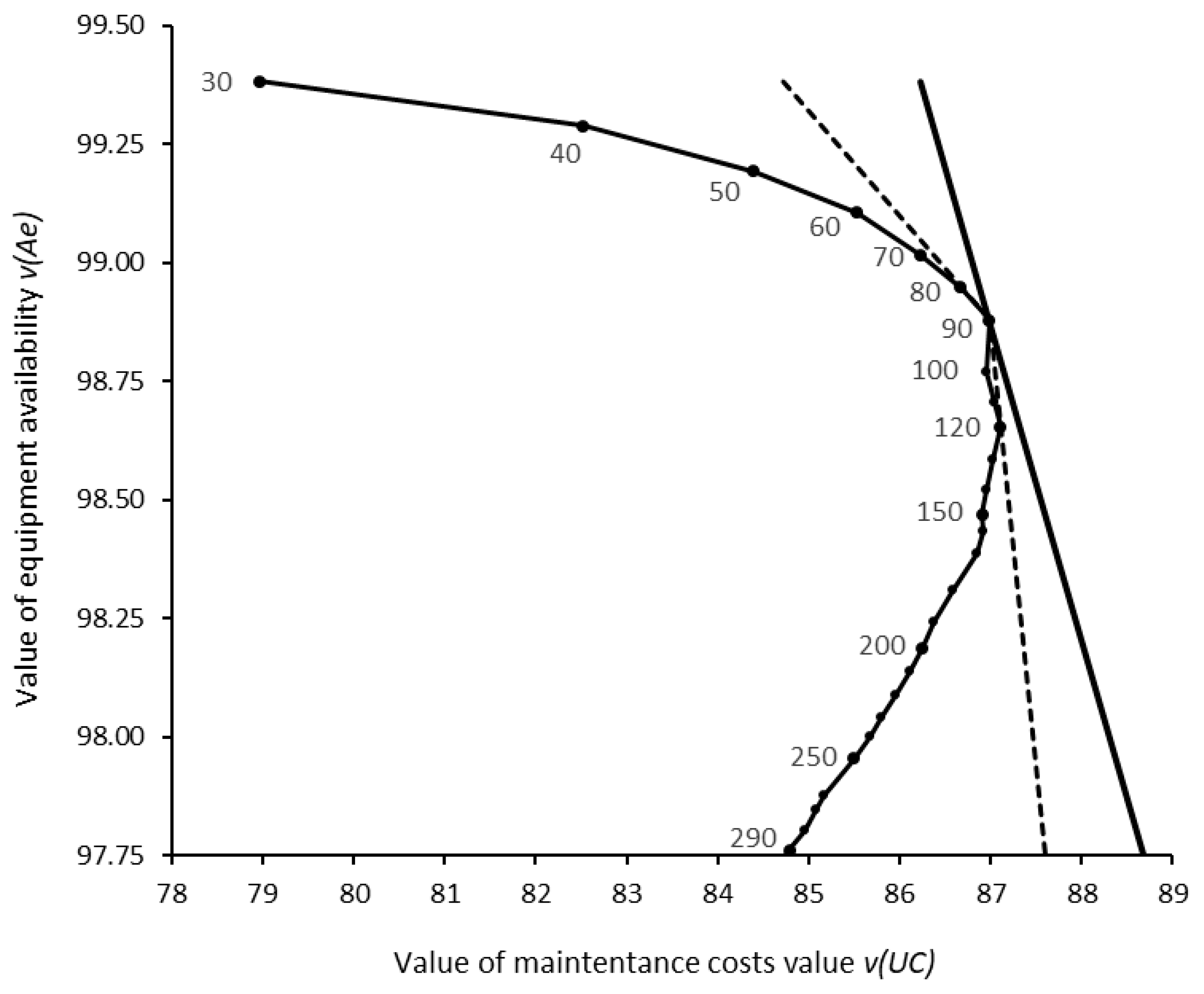
A sensitivity analysis on the weights allowed to verify their impact on the selection of the optimal inspection period from the set of inspection periods ranging from 30 to 300 hours in increments of 10 hours. It was found that the selection of = 90 hours is robust to changes in between 18% and 65%, and, consequently, to changes in between 35% and 82%. These variations correspond to an interval between 3300 and 27000 €/100 hours (rather than 9000) regarding the amount that the organization is willing to pay for improving equipment availability from 0% to 100%, suggesting that the decision is indeed robust. Figure 16 plots the efficient frontier connecting the partial values and of all evaluated inspection periods along with the isoline representing the optimal overall value with =40% and =60%. Dashed lines represent the two iso-value lines for the weights that change the optimal inspection period from 90 hours to: a) 80 hours, when =18% and =82%; b) 120 hours, when =65% and =35%.
5. Discussion
This study introduces a novel, integrated, generic multimethodological approach for determining the optimal inspection period for protective sensors monitoring critical equipment. It considers multiple KPIs and the uncertainty associated with hidden failures in the system and the organization’s preferences. A case study illustrating the application of the proposed approach to a real-world maintenance problem via a DSS demonstrates its practical applicability and contributes to the limited body of proactive maintenance modeling and optimization research applied in practice [19].
The modeling approach and DSS were developed to answer the five key research questions, identified in the Introduction, and commonly encountered in real-work applications of this maintenance problem. The results demonstrate that the proposed solution effectively addresses each specific research question as follows:
- The use of three-parameter Weibull probability density functions, Monte Carlo simulation, and the principles of the Probability Management discipline enable an effective and auditable representation of the uncertainties related to failures in the equipment and sensor;
- Discrete-event simulation modeling allows for accurate prediction of the consequences of these failures on multiple KPIs considering varying sensor inspection periods, costs, time periods, and other input parameters;
- Risk analysis and value-based multicriteria decision analysis methods facilitate risk-informed assessment of the overall value of different sensor inspection periods considering both their uncertain consequences and the preferences of the organization on multiple conflicting organizational KPIs, namely by representing the intertemporal, intra-criterion, and inter-criteria preferences of the organization through discount rate, value functions, and weights of the KPIs, respectively;
- Risk-informed multicriteria value optimization methods, namely stochastic dominance and/or expected value maximization, provide a sound criterion for determining the optimal inspection period, while sensitivity analysis allows to assess the robustness of the optimal decision against the uncertainty of the organization’s preferences;
- Finally, organizational buy-in and the successful implementation of maintenance decisions recommended by a decision support model require not only the scientific rigor and integration of the underlying approach, but also key success factors related to the DSS, such as its transparency, openness, understandability, user-friendliness, and auditability. These qualities were ensured by developing a prototype in Microsoft Excel, utilizing only built-in functions and taking advantage of the principles of Probability Management.
This research addresses a significant gap in the maintenance literature regarding the need for integrated methodologies that combine quantitative and qualitative data, uncertainty and risk analysis, and organizational preferences across multiple KPIs. The proposed framework contributes to the state-of-the-art by providing a practical and robust approach to optimizing inspection scheduling for protective sensors monitoring critical equipment subject to uncertain hidden failures. In contrast to traditional maintenance models, which often rely on simplified assumptions and deterministic approaches, this framework explicitly accounts for the uncertainty associated with sensor and equipment failures as well as organizational preferences, aligning with recommendations for more risk-informed multicriteria decision-making in industrial maintenance.
Another strength of the proposed approach is its generic nature, enabling it to accommodate different parameters and integrate additional assumptions, such as incorporating new KPIs, using alternative probability distributions for modeling failure uncertainty, or applying other MCVM methods for determining intra-criterion and/or inter-criteria preferences.
Another key contribution to practice is the development and provision of an open-access DSS in Excel, making it valuable for understanding, teaching, and supporting practical decision-making in related maintenance problems.
The main limitations of the results include the following. The computational time required to run a large number of simulations, which were significantly reduced, from several hours to several minutes, by using the Table Data feature from Excel instead of VBA macros, but that still demand several minutes to run when there are thousands of simulations as in the case study presented in this article. Another limitation regards the comparison of discrete inspect periods only, which might miss a better inspection period compared to the continuous case. One solution to this limitation comprises running the same problem again with a set of less evenly spaced inspection periods around the previous optimal inspection period. For instance, in the presented case study, running the DSS again with the optimization input parameters set with a minimum of 80 hours, maximum of 100 hours, and step of 1 hour. Minor limitations, which can be easily addressed by model refinement, include: modeling sensor inspection time if the sensor is not available to perform its protecting function while the inspection is performed; and modeling probabilistically the duration and/or costs of other maintenance tasks, namely regarding inspection, repair, and reactivation.
6. Conclusions
This research provides a novel, integrated, generic multimethodological approach for determining the optimal inspection period of protective sensors monitoring critical equipment subject to hidden failures. The proposed approach addresses the underlying research questions required to tackle this maintenance problem by: (a) modeling failure uncertainties using probability density functions, Monte Carlo simulation, and Probability Management: (b) predicting failure consequences on KPIs through discrete-event simulation; (c) comparing the overall value of alternative inspection periods using multicriteria value measurement and risk analysis methods; (d) determining the optimal inspection period considering uncertainties and preferences by stochastic dominance, expected value maximization, and sensitivity analysis; and (e) developing a user-friendly decision support system for practical implementation.
The key finding is that optimal inspection periods can be effectively determined considering varying uncertainties, multiple KPIs, and specific organizational preferences and risk attitudes.
The developed framework and decision support system empower organizations to make risk-informed multicriteria decisions regarding sensor inspection schedules, leading to optimized industrial maintenance. This translates to reduced downtime, lower maintenance costs, and improved overall equipment effectiveness. The proposed integrated approach represents an advancement over traditional methods that often rely on simplified assumptions and single-criteria optimization. The methodology is readily applicable across various industries reliant on critical equipment with protective sensors, such as power generation, manufacturing, and transportation. By adopting this approach, organizations can enhance their proactive maintenance practices and improve operational efficiency.
Future research should explore the integration of real-time condition monitoring data into the proposed approach, allowing for even more dynamic and adaptive inspection schedules. Further investigation into the scalability of the framework for modelling complex networks with multiple protective sensors interconnected with critical equipment can also offer valuable insights. Two sensors can be either used as a protective function or one replace the other while it is being repaired, providing redundancy but with additional costs. Additionally, exploring the relevance of modeling non-neutral risk attitudes on the optimal inspection period could be investigated. We encourage researchers and practitioners to adopt and adapt this framework to their specific contexts, contributing to the advancement of proactive maintenance practices and improved asset management.
Supplementary Materials
The following supporting information can be downloaded at: https://www.mdpi.com/article/doi/s1, Prototype Excel application mentioned in the Case Study.
Author Contributions
Conceptualization, R.J.G.M. and R.A.; methodology, R.J.G.M. and R.A.; software, R.J.G.M. and R.A.; validation, All authors; writing—original draft preparation, R.J.G.M. and R.A.; writing—review and editing, P.C.M., A.D.B.M., J.C.A.R and F.S.P.; All authors have read and agreed to the published version of the manuscript.
Funding
This research received no external funding.
Abbreviations
The following abbreviations are used in this manuscript:
| a.k.a. | also known as |
| DSS | Decision support system |
| KPI | Key performance indicator |
| MCVM | Multicriteria value measurement methods |
| MTBF | Mean time between failures |
| MTTF | Mean time to failure |
| MTTR | Mean time to repair |
| RCM | Reliability centered maintenance |
| VBA | Visual basic for applications |
References
- SIEMENS The True Cost of Downtime 2024.
- SAE JA1012 A Guide to the Reliability-Centered Maintenance (RCM) Standard; 2002.
- Moubray, J. Reliability-Centred Maintenance; 2. ed.; Elsevier: Amsterdam Heidelberg, 2004; ISBN 978-0-7506-3358-1. [Google Scholar]
- Zhang, Y.; Ouyang, L.; Meng, X.; Zhu, X. Condition-Based Maintenance Considering Imperfect Inspection for a Multi-State System Subject to Competing and Hidden Failures. Comput. Ind. Eng. 2024, 188, 109856. [Google Scholar] [CrossRef]
- Tang, T.; Lin, D.; Banjevic, D.; Jardine, A.K.S. Availability of a System Subject to Hidden Failure Inspected at Constant Intervals with Non-Negligible Downtime Due to Inspection and Downtime Due to Repair/Replacement. J. Stat. Plan. Inference 2013, 143, 176–185. [Google Scholar] [CrossRef]
- Alsyouf, I. The Role of Maintenance in Improving Companies’ Productivity and Profitability. Int. J. Prod. Econ. 2007, 105, 70–78. [Google Scholar] [CrossRef]
- Ahmed Murtaza, A.; Saher, A.; Hamza Zafar, M.; Kumayl Raza Moosavi, S.; Faisal Aftab, M.; Sanfilippo, F. Paradigm Shift for Predictive Maintenance and Condition Monitoring from Industry 4.0 to Industry 5.0: A Systematic Review, Challenges and Case Study. Results Eng. 2024, 24, 102935. [Google Scholar] [CrossRef]
- Zhu, T.; Ran, Y.; Zhou, X.; Wen, Y. A Survey of Predictive Maintenance: Systems, Purposes and Approaches 2019.
- Shen, J.; Hu, J.; Ma, Y. Two Preventive Replacement Strategies for Systems with Protective Auxiliary Parts Subject to Degradation and Economic Dependence. Reliab. Eng. Syst. Saf. 2020, 204, 107144. [Google Scholar] [CrossRef]
- Taghipour, S.; Banjevic, D.; Jardine, A.K.S. Periodic Inspection Optimization Model for a Complex Repairable System. Reliab. Eng. Syst. Saf. 2010, 95, 944–952. [Google Scholar] [CrossRef]
- Rodrigues, J.A.; Farinha, J.T.; Cardoso, A.M.; Mendes, M.; Mateus, R. Prediction of Sensor Values in Paper Pulp Industry Using Neural Networks. In Proceedings of IncoME-VI and TEPEN 2021; Zhang, H., Feng, G., Wang, H., Gu, F., Sinha, J.K., Eds.; Mechanisms and Machine Science; Springer International Publishing: Cham, 2023; Vol. 117, pp. 281–291. ISBN 978-3-030-99074-9. [Google Scholar]
- Rodrigues, J.A.; Farinha, J.T.; Mendes, M.; Mateus, R.J.G.; Cardoso, A.J.M. Comparison of Different Features and Neural Networks for Predicting Industrial Paper Press Condition. Energies 2022, 15, 6308. [Google Scholar] [CrossRef]
- Rodrigues, J.A.; Martins, A.; Mendes, M.; Farinha, J.T.; Mateus, R.J.G.; Cardoso, A.J.M. Automatic Risk Assessment for an Industrial Asset Using Unsupervised and Supervised Learning. Energies 2022, 15, 9387. [Google Scholar] [CrossRef]
- Rodrigues, J.; Farinha, J.; Mendes, M.; Mateus, R.; Cardoso, A. Short and Long Forecast to Implement Predictive Maintenance in a Pulp Industry. Eksploat. Niezawodn. – Maint. Reliab. 2022, 24, 33–41. [Google Scholar] [CrossRef]
- Nowlan, F.S.; Heap, H.F. Reliability-Centered Maintenance; U.S. Department of Commerce, 1978.
- Roux, M.; Fang, Y.-P.; Barros, A. Impact of Imperfect Monitoring on the Optimal Condition-Based Maintenance Policy of a Single-Item System. In Proceedings of the Book of Extended Abstracts for the 32nd European Safety and Reliability Conference; Research Publishing Services, 2022; pp. 658–664.
- Zhao, X.; Guo, B.; Chen, Y. A Condition-Based Inspection-Maintenance Policy for Critical Systems with an Unreliable Monitor System. Reliab. Eng. Syst. Saf. 2024, 242, 109710. [Google Scholar] [CrossRef]
- Alaswad, S.; Xiang, Y. A Review on Condition-Based Maintenance Optimization Models for Stochastically Deteriorating System. Reliab. Eng. Syst. Saf. 2017, 157, 54–63. [Google Scholar] [CrossRef]
- De Jonge, B.; Scarf, P.A. A Review on Maintenance Optimization. Eur. J. Oper. Res. 2020, 285, 805–824. [Google Scholar] [CrossRef]
- Assis, R.; Marques, P.C. A Dynamic Methodology for Setting Up Inspection Time Intervals in Conditional Preventive Maintenance. Appl. Sci. 2021, 11, 8715. [Google Scholar] [CrossRef]
- Werbińska-Wojciechowska, S. Inspection Models for Technical Systems. In Technical System Maintenance; Springer Series in Reliability Engineering; Springer International Publishing: Cham, 2019; pp. 101–159 . ISBN 978-3-030-10787-1. [Google Scholar]
- Trade-off Analytics: Creating and Exploring the System Tradespace; Parnell, G.S., Ed.; Wiley series in systems engineering and management; Wiley: Hoboken, New Jersey, 2017; ISBN 978-1-119-23753-2. [Google Scholar]
- Ruschel, E.; Santos, E.A.P.; Loures, E.D.F.R. Industrial Maintenance Decision-Making: A Systematic Literature Review. J. Manuf. Syst. 2017, 45, 180–194. [Google Scholar] [CrossRef]
- Tang, T. Failure Finding Interval Optimization for Periodically Inspected Repairable Systems. PhD Thesis, University of Toronto, 2012.
- Ten Wolde, M.; Ghobbar, A.A. Optimizing Inspection Intervals—Reliability and Availability in Terms of a Cost Model: A Case Study on Railway Carriers. Reliab. Eng. Syst. Saf. 2013, 114, 137–147. [Google Scholar] [CrossRef]
- Tian, Z.; Lin, D.; Wu, B. Condition Based Maintenance Optimization Considering Multiple Objectives. J. Intell. Manuf. 2012, 23, 333–340. [Google Scholar] [CrossRef]
- Ferreira, R.J.P.; De Almeida, A.T.; Cavalcante, C.A.V. A Multi-Criteria Decision Model to Determine Inspection Intervals of Condition Monitoring Based on Delay Time Analysis. Reliab. Eng. Syst. Saf. 2009, 94, 905–912. [Google Scholar] [CrossRef]
- Park, M.; Lim, J.-H.; Kim, D.-K.; Kim, J.-W.; Park, D.H.; Park, B.-N.; Park, J.H.; Song, M.-O.; Sung, S.-I.; Jung, K.M. A Study to Determine Optimal Inspection Intervals Using a Multi-Criteria Decision Model. J. Appl. Reliab. 2021, 21, 282–293. [Google Scholar] [CrossRef]
- Zhao, X. Multi-Criteria Decision Model for Imperfect Maintenance Using Multi-Attribute Utility Theory. Int. J. Perform. Eng. 2018. [CrossRef]
- OREDA Offshore Reliability Data Handbook; 4th ed. ; OREDA Participants: Distributed by Der Norske Veritas: Høvik, Norway, 2002; ISBN 978-82-14-02705-1.
- Belton, V.; Stewart, T.J. Multiple Criteria Decision Analysis: An Integrated Approach; Springer US, 2002; ISBN 978-1-4613-5582-3.
- Kirkwood, C.W. Strategic Decision Making: Multiobjective Decision Analysis with Spreadsheets; Duxbury Press: Belmont, 1997; ISBN 978-0-534-51692-5. [Google Scholar]
- Goodwin, P.; Wright, G. Decision Analysis for Management Judgment; 5th Edition.; Wiley: Hoboken, New Jersey, 2014; ISBN 978-1-118-74073-6. [Google Scholar]
- Mateus, R.; Ferreira, J.A.; Carreira, J. Full Disclosure of Tender Evaluation Models: Background and Application in Portuguese Public Procurement. J. Purch. Supply Manag. 2010, 16, 206–215. [Google Scholar] [CrossRef]
- Winterfeldt, D. von; Edwards, W. Decision Analysis and Behavioral Research; Repr.; Cambridge Univ. Press: Cambridge, 1993; ISBN 978-0-521-27304-6. [Google Scholar]
- Bana E Costa, C. MACBETH — An Interactive Path towards the Construction of Cardinal Value Functions. Int. Trans. Oper. Res. 1994, 1, 489–500. [Google Scholar] [CrossRef]
- Keeney, R.L.; Raiffa, H. Decisions with Multiple Objectives: Preferences and Value Trade-Offs; 1st ed.; Cambridge University Press, 1993; ISBN 978-0-521-43883-4.
- Bana e Costa, C.A.; Vansnick, J.-C. Applications of the MACBETH Approach in the Framework of an Additive Aggregation Model. J. Multi-Criteria Decis. Anal. 1997, 6, 107–114. [Google Scholar] [CrossRef]
- Clemen, R.T.; Reilly, T. Making Hard Decisions with Decision Tools; 3., rev. ed.; South-Western/Cengage Learning: Mason, Ohio, 2014; ISBN 978-0-538-79757-3. [Google Scholar]
- Savage, S.L. The Flaw of Averages: Why We Underestimate Risk in the Face of Uncertainty; John Wiley & Sons, Inc: Hoboken, New Jersey, 2012; ISBN 978-1-118-07375-9. [Google Scholar]
- Probability Management. Available online: https://www.probabilitymanagement.org/ (accessed on 16 December 2024).
Figure 1.
Diagram logic of the methodology.
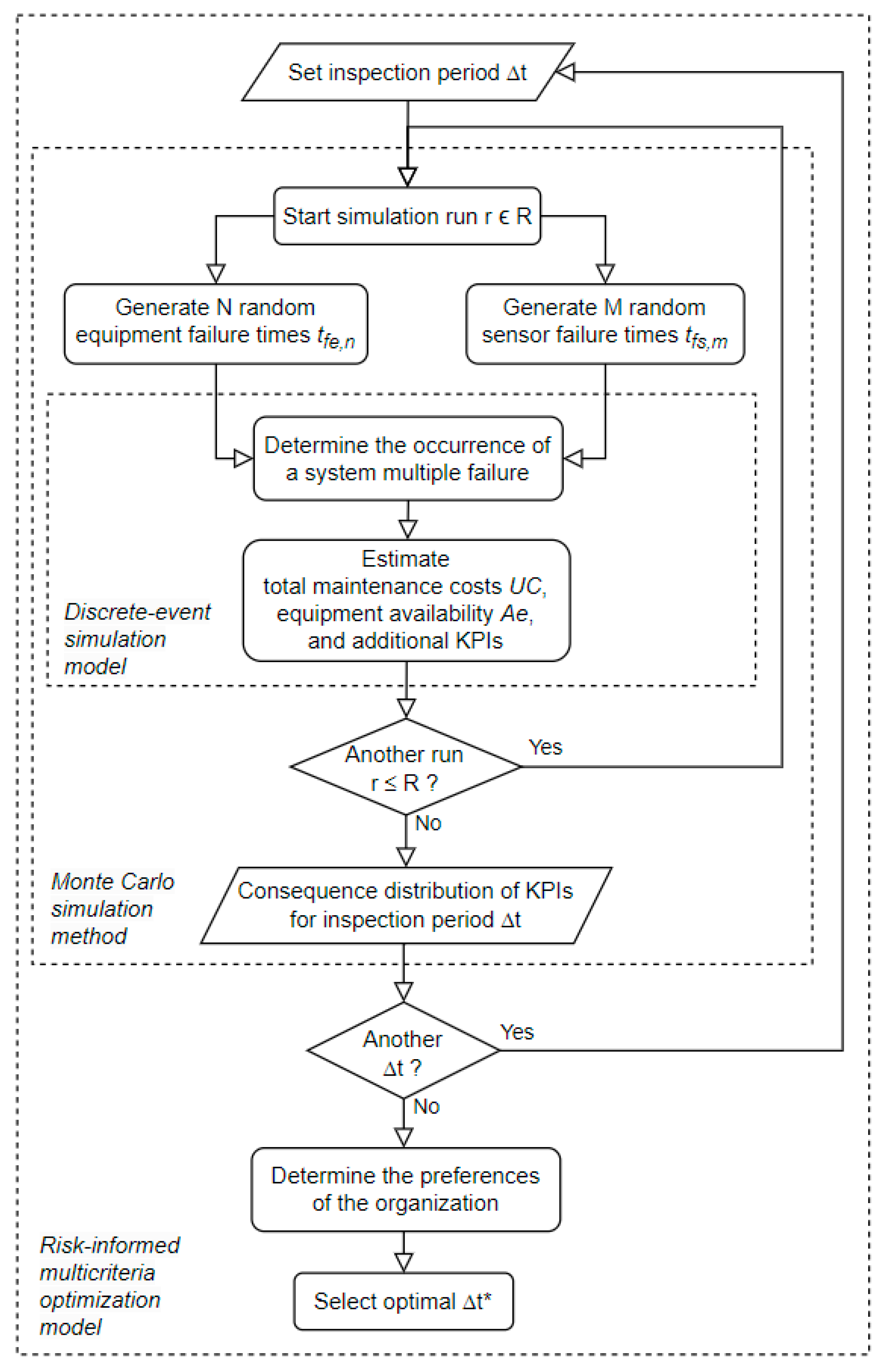
Figure 2.
Probability density f(t) and cumulative distribution F(t) functions of the Weibull distribution.
Figure 2.
Probability density f(t) and cumulative distribution F(t) functions of the Weibull distribution.
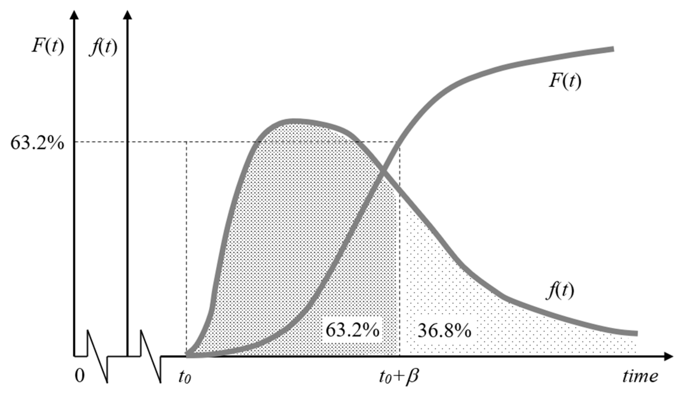
Figure 3.
Conditional probability of failure in time period having already survived until time .
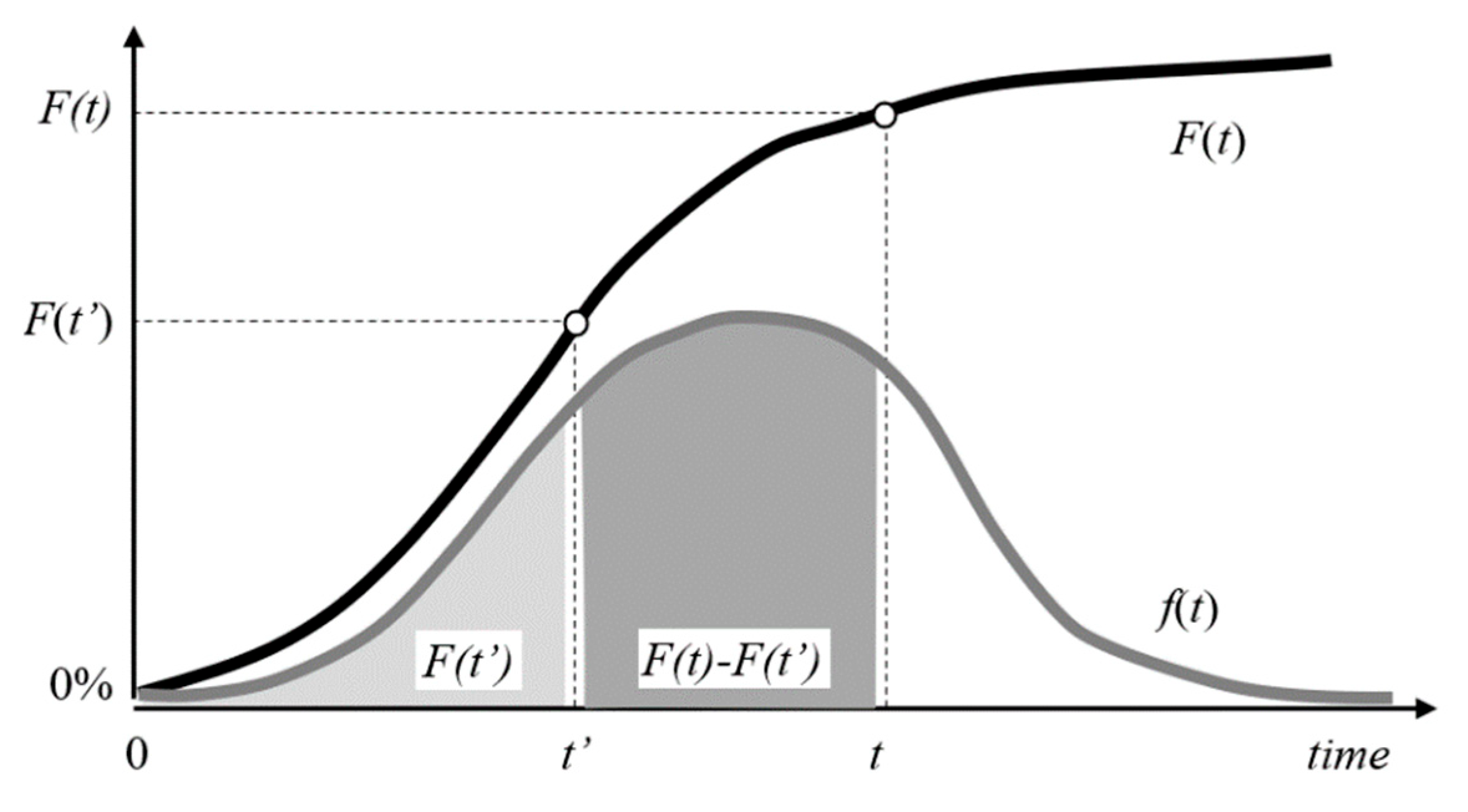
Figure 4.
Discrete-event simulation model to find the system multiple failure time.

Figure 5.
DSS implemented in a Portuguese electric utility organization.
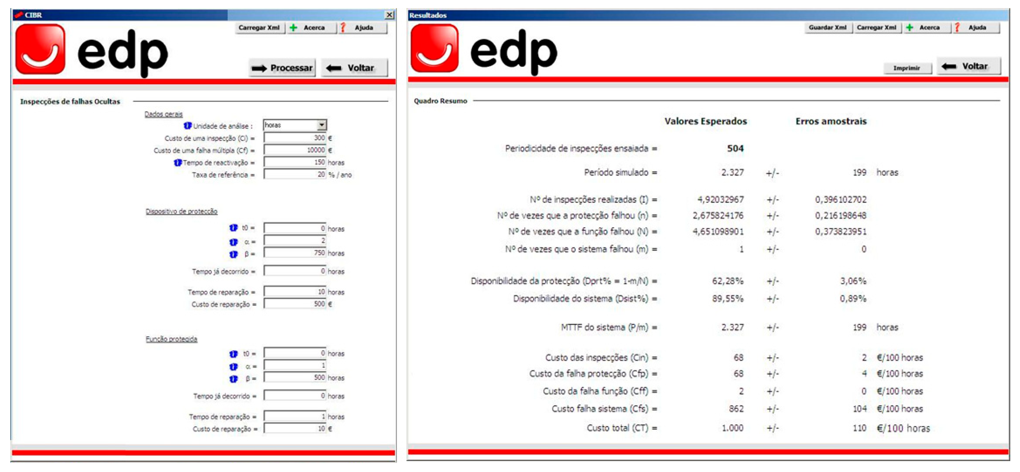
Figure 6.
User inputs interface (sheet “Inputs”).
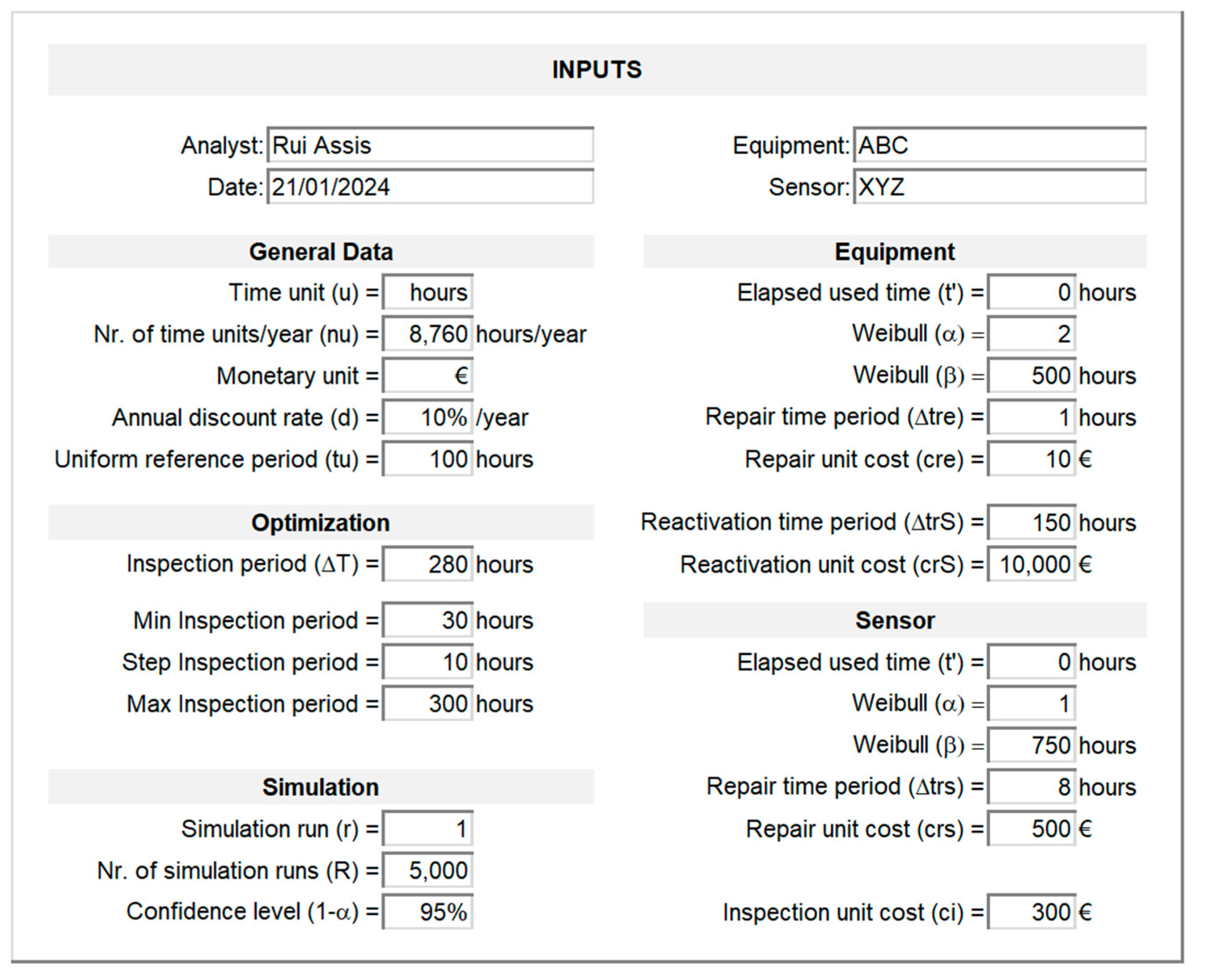
Figure 7.
Sensor random failure times interface (sheet “Sensor”).
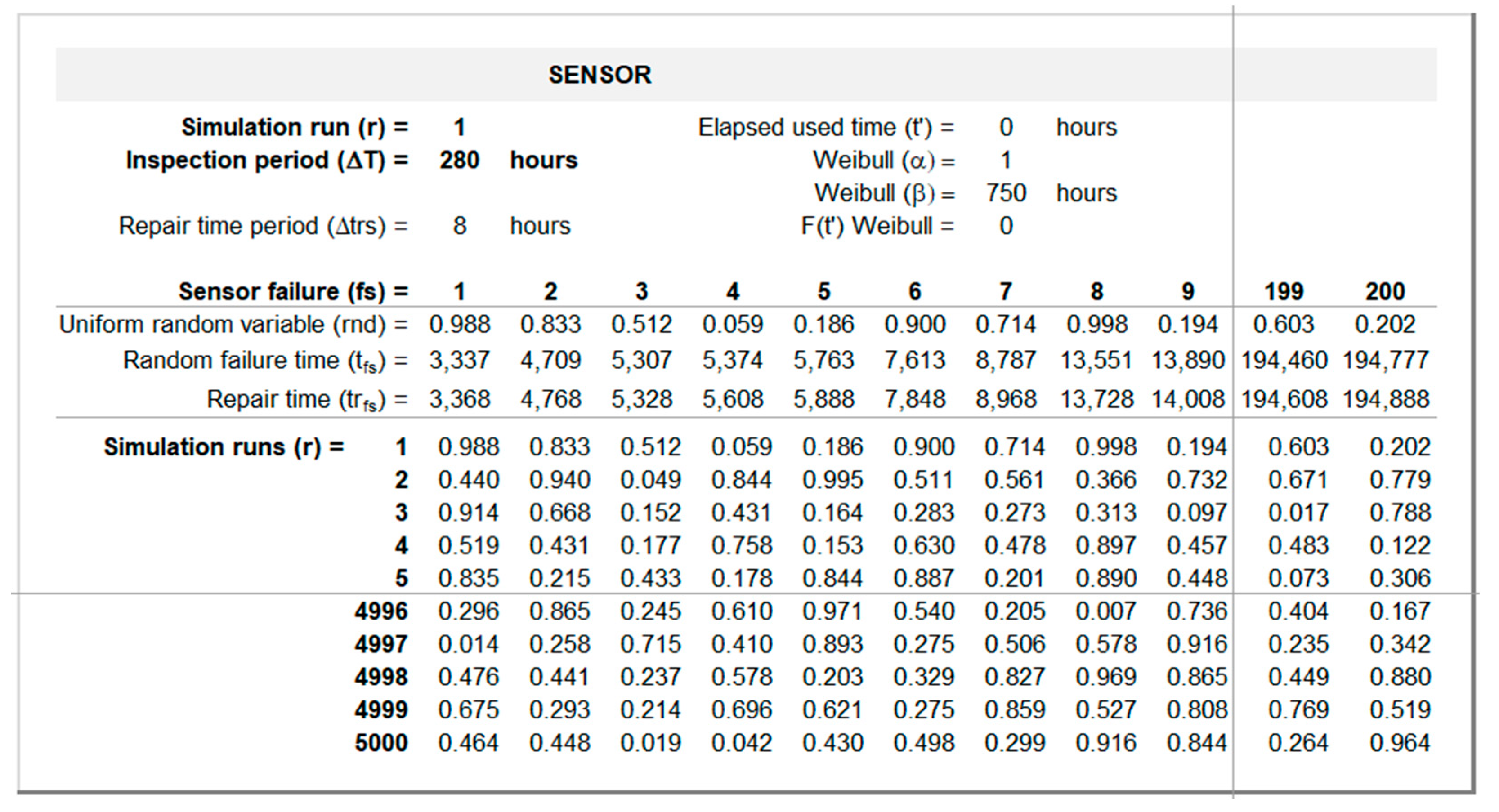
Figure 8.
Equipment random failure interface (sheet “Equipment”).
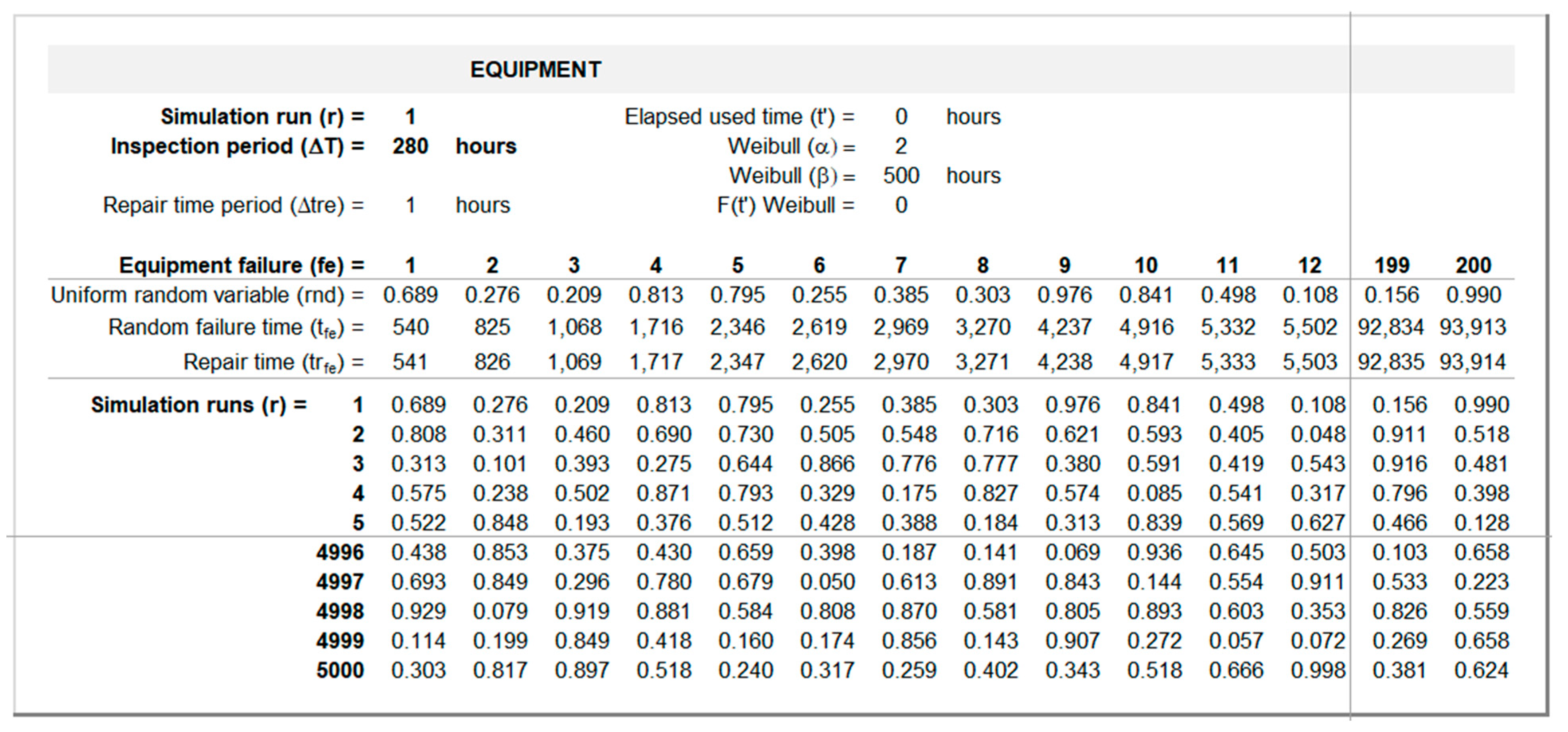
Figure 9.
System (multiple) failure and KPIs interface (sheet “System”).
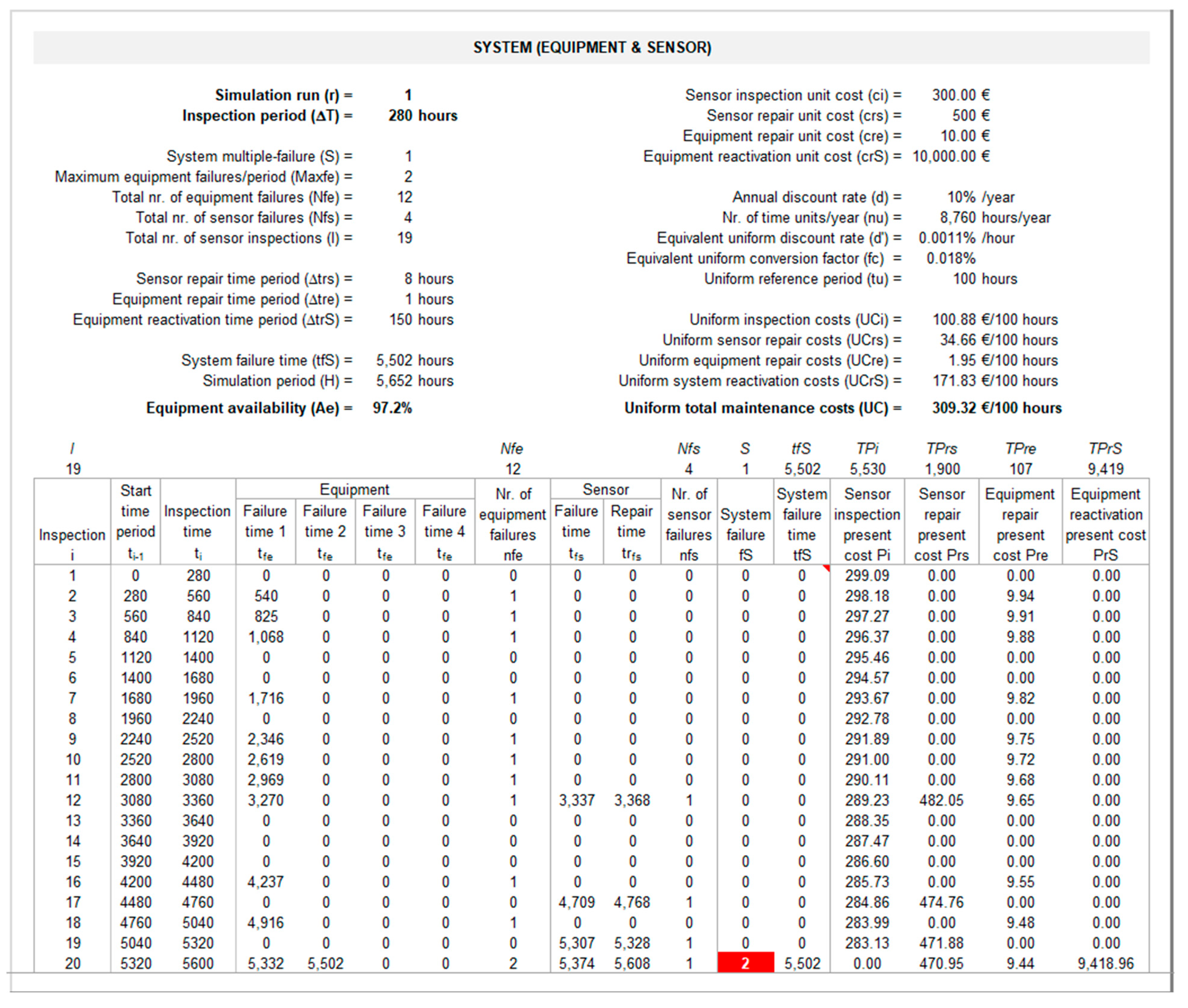
Figure 10.
Total maintenance costs across 5000 runs for inspection periods
=30 to 300 hours.
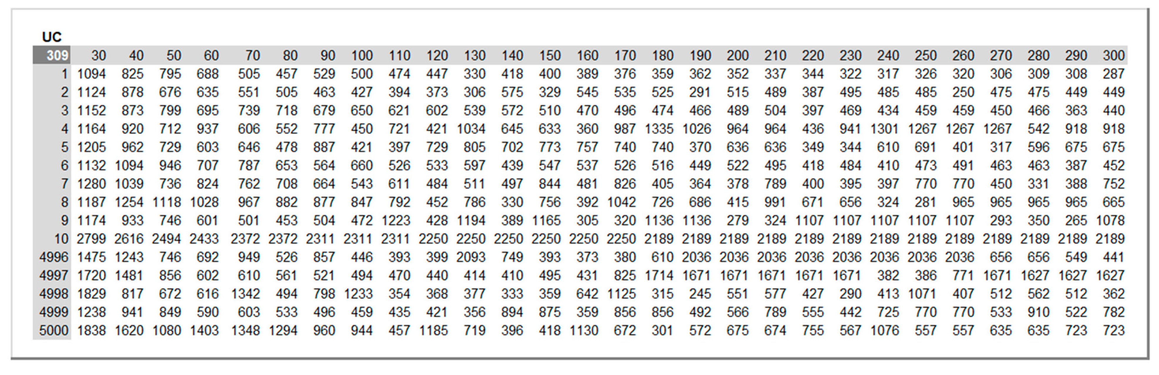
Figure 11.
Equipment availability across 5000 runs for inspection periods
=30 to 300 hours.
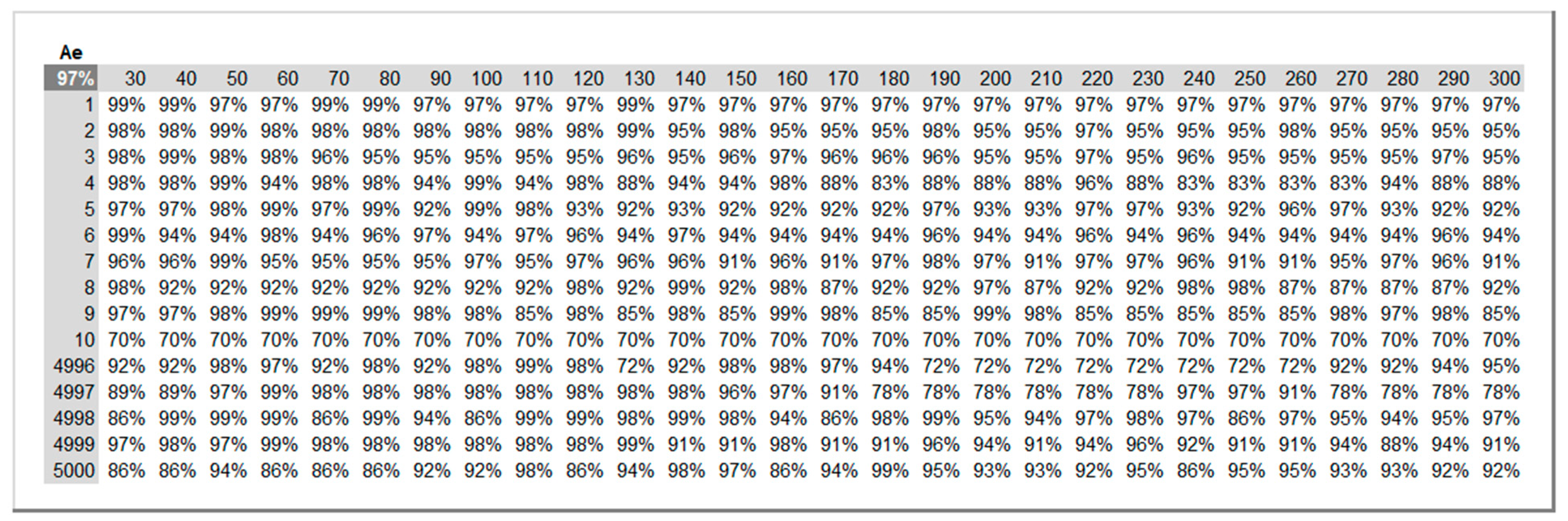
Figure 12.
Expected values and 95% confidence intervals of maintenance costs ( ) for inspection periods
=30 to 300 hours computed from 5000 simulation runs.
Figure 12.
Expected values and 95% confidence intervals of maintenance costs ( ) for inspection periods
=30 to 300 hours computed from 5000 simulation runs.
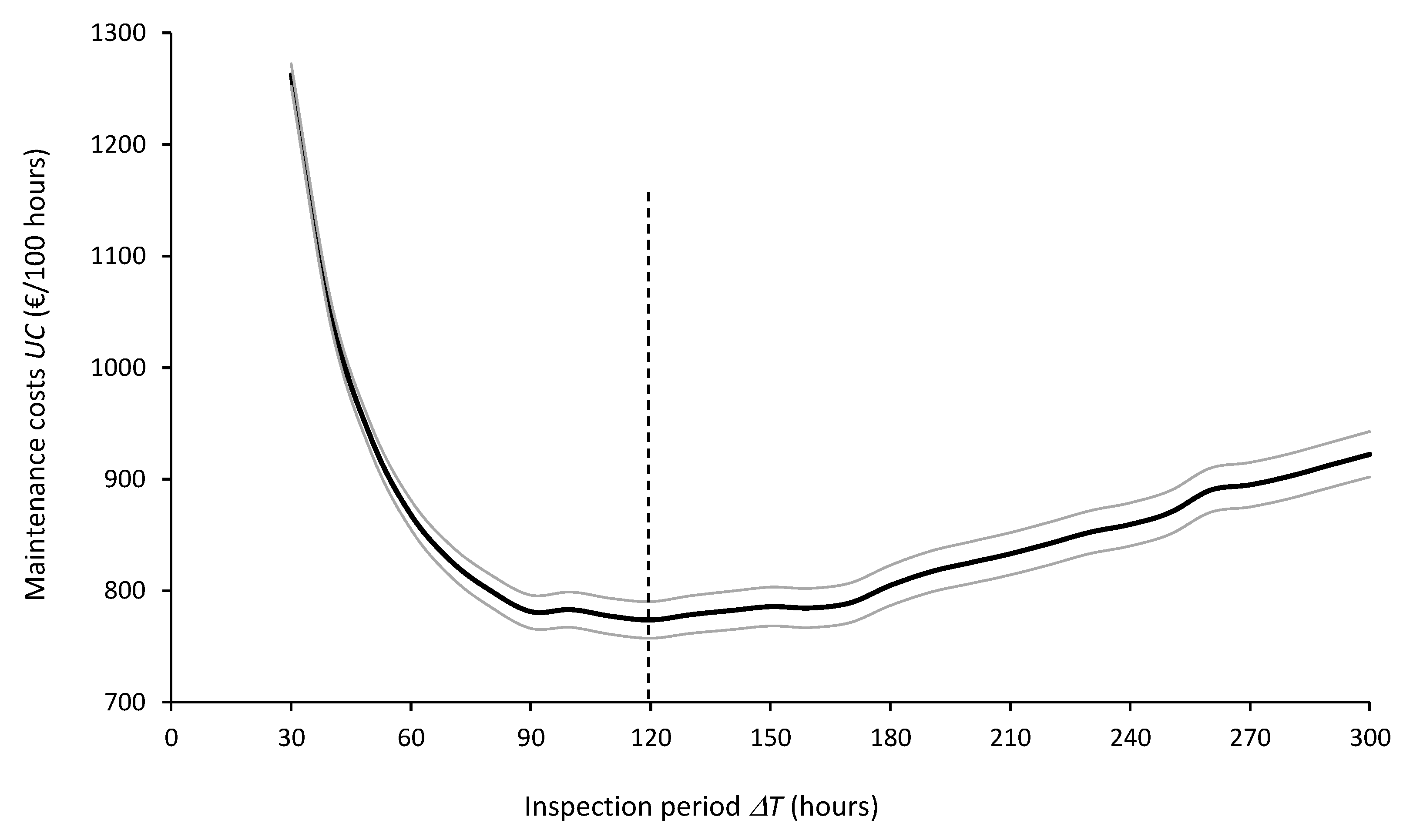
Figure 13.
Expected values and 95% confidence intervals of equipment availability ( ) for inspection periods
=30 to 300 hours computed from 5000 simulation runs.
Figure 13.
Expected values and 95% confidence intervals of equipment availability ( ) for inspection periods
=30 to 300 hours computed from 5000 simulation runs.
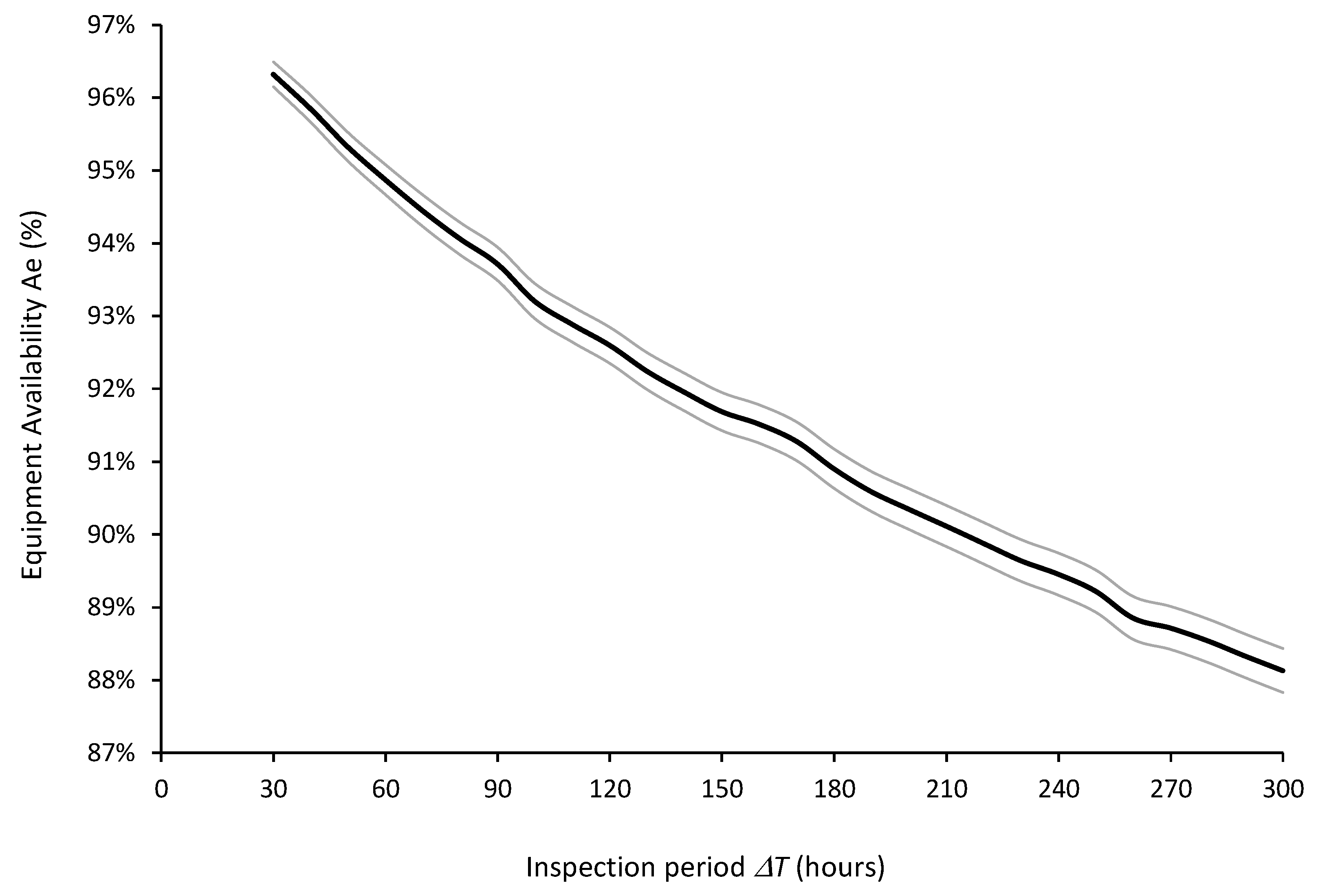
Figure 14.
Cumulative risk profiles for the overall value of inspection periods
= 30, 50, 70, 90, 120, and 300 hours (The x-axis was truncated before 75 to enhance clarity).
Figure 14.
Cumulative risk profiles for the overall value of inspection periods
= 30, 50, 70, 90, 120, and 300 hours (The x-axis was truncated before 75 to enhance clarity).
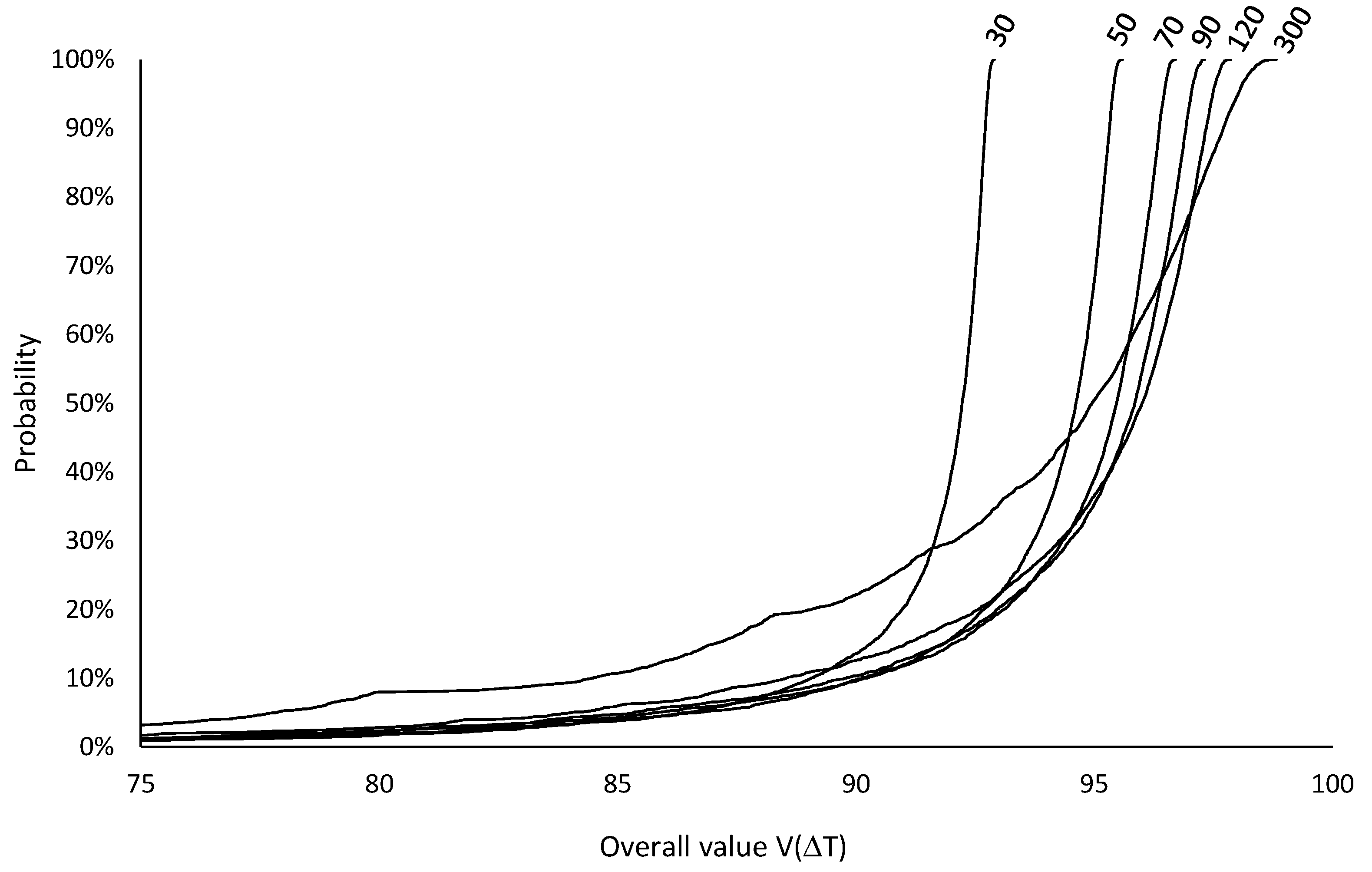
Figure 15.
Expected values and 95% confidence intervals of overall value for inspection periods
=30 to 300 hours from 5000 simulation runs.
Figure 15.
Expected values and 95% confidence intervals of overall value for inspection periods
=30 to 300 hours from 5000 simulation runs.
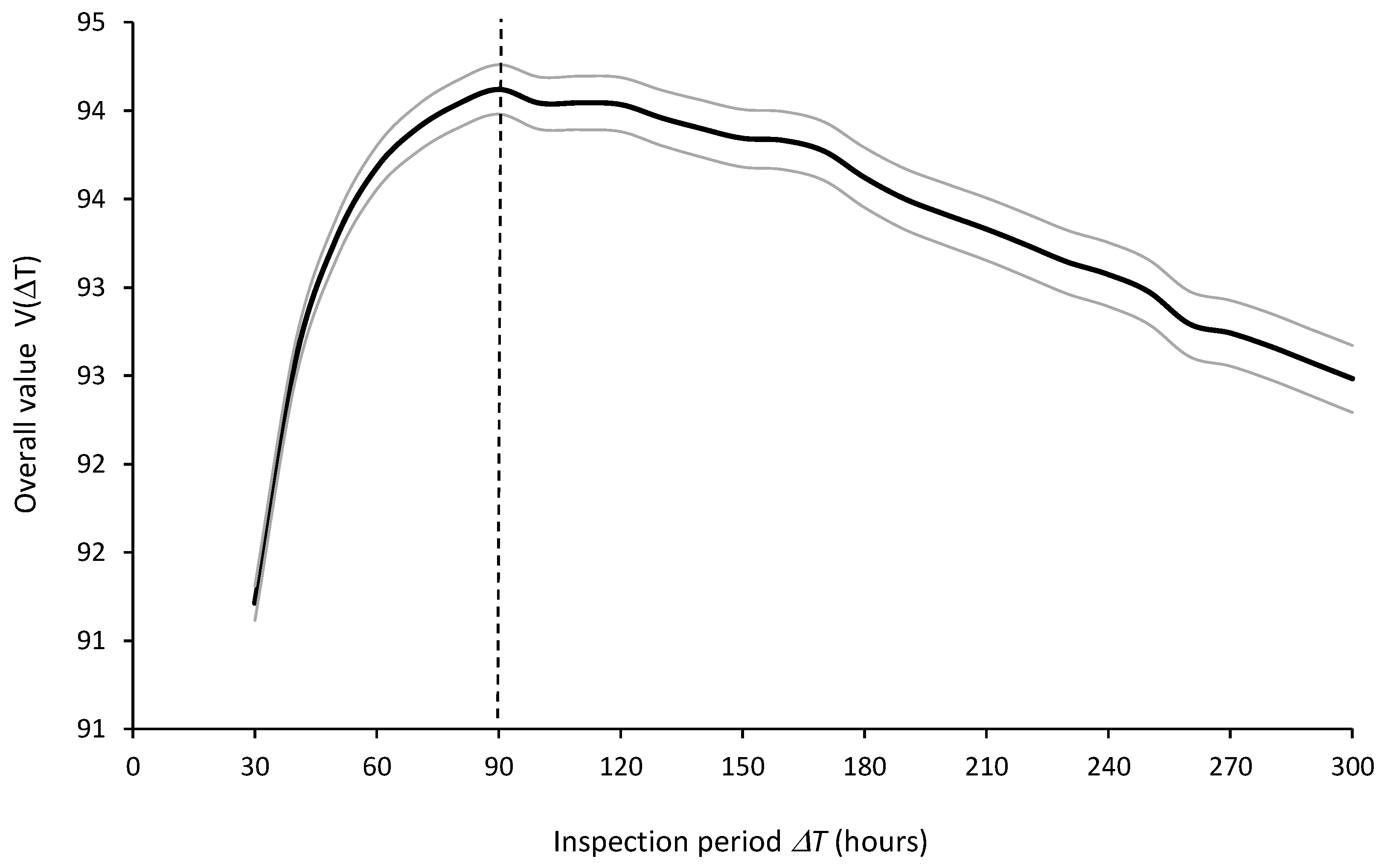
Figure 16.
KPI value space. Dotted curve represents the values and
of inspection periods
=30 to 300 hours. Solid line is the optimal
. Dashed lines represent
and
.
Figure 16.
KPI value space. Dotted curve represents the values and
of inspection periods
=30 to 300 hours. Solid line is the optimal
. Dashed lines represent
and
.
Disclaimer/Publisher’s Note: The statements, opinions and data contained in all publications are solely those of the individual author(s) and contributor(s) and not of MDPI and/or the editor(s). MDPI and/or the editor(s) disclaim responsibility for any injury to people or property resulting from any ideas, methods, instructions or products referred to in the content. |
© 2025 by the authors. Licensee MDPI, Basel, Switzerland. This article is an open access article distributed under the terms and conditions of the Creative Commons Attribution (CC BY) license (http://creativecommons.org/licenses/by/4.0/).
Copyright: This open access article is published under a Creative Commons CC BY 4.0 license, which permit the free download, distribution, and reuse, provided that the author and preprint are cited in any reuse.


