
Submitted:
04 June 2025
Posted:
05 June 2025
You are already at the latest version
Abstract
Combustion modelling using computational fluid dynamics offers detailed insights on the flame structure and thermo-chemical processes. Furthermore, CFD is extensively used in the past to optimize industrial furnaces. Despite the increasing computational power, the prediction of the reaction kinetics in flames is still related to high calculation times, which is a major drawback for large scale combustion systems. To speed-up the simulation, artificial neural networks (ANNs) were applied in this study to calculate the chemical source terms in the flame instead of using a chemistry solver. Since one ANN may lack of accuracy for the entire input feature space (temperature, species concentrations), the space is subdivided in 4 regions/ANNs. The ANNs were tested for different fuel mixtures, degrees of turbulence and air-fuel/oxy-fuel combustion. It was found that the shape of the flame and its position was well predicted in all cases with regard to the temperature and CO. However, at low temperature levels (< 800 K) in some cases the ANNs under-predicted the source terms. Additionally, in oxy-fuel combustion the temperature was too high. Nevertheless, an overall high accuracy and a speed-up factor for all simulations of 12 was observed, which makes the approach highly suitable for large scale furnaces.
Keywords:
Combustion modelling
; Eddy dissipation concept
; Artificial neural networks
; Computational fluid dynamics
; Hydrogen combustion
; Oxygen enhanced combustion
; Hybrid modelling
; Machine learning
1. Introduction
Combustion processes at temperatures above 1000°C (e.g., gas turbines [1], steel reheating furnaces [2], glass melting [3]) as well as other reactive flows at moderate temperature levels (e.g., solid oxide fuel cells [4]) and (near) ambient conditions (e.g., bioreactors [5]) are essential for modern society to produce high-tech products or products for daily life. Modelling the reactive flow using computational fluid dynamics (CFD) simulation needs the consideration of the chemical reactions over time, which means that in addition to the transport equations for the continuity and momentum also the energy equation and transport equations for the chemical species (or a related quantity such as the mixture fraction) have to be solved. Additionally, at high temperatures also the radiative transport equation has to be considered. With regard to combustion processes the determination of the chemical reactions and the radiative heat transfer represent the highest computational demand. Considering the chemistry calculation, Mao et al. [6] presented the performance of three hardware configurations on the CFD simulation of a 2D Taylor-Green vortex. It was found that the chemistry step needs the majority of the calculation time compared to the other transport equations. Since the calculation of the reaction kinetics during combustion processes is crucial for the overall calculation time, many chemistry solvers were published in the past trying to effectively predict the chemistry, such as Cantera [7] or CVODE [8]. Cuoci et al. [9], with their OpenSMOKE++ framework, were able to accelerate the chemistry calculation where the required time for solving the reaction kinetics now equals the transport step in the simulation. However, it was found that the performance of the ODE solvers for the chemistry are sensitive to the used reaction mechanism. Nevertheless, the prediction of the reaction kinetic within a flame or the numerical cell is still a crucial point in combustion simulation, especially when it comes to direct numerical simulation (DNS) for micro-scale modelling of turbulent flames or large domains (e.g., industrial furnaces, gas turbines), where commonly large eddy simulation (LES) or simulations based on the RANS (Reynolds-averaged Navier-Stokes) are used. Reducing the calculation time in the chemistry step would significantly improve the applicability of CFD simulations for the analysis of combustion processes. One method to address this issue, which was applied by researchers recently, is the usage of artificial neural networks (ANNs). It was already shown by Kalogirou [10] back in 2003, that techniques based on artificial intelligence (AI) can be helpful in understanding combustion and were later used to monitor the combustion behavior in furnaces (e.g., [11,12,13]). Since the response of ANNs for the prediction of chemical kinetics is significantly faster than its calculation, it makes sense to use and implement them in CFD simulations of reactive flows (especially combustion).
In CFD simulations of reactive flows or combustion processes the species transport equation (see equation 1) has to be solved, where is the density, is the species mass fraction of the species , is the time, is the velocity vector, is the diffusion velocity of the species and is the reaction rate of the species . The reaction rates are predicted by the chemistry solver. In the case of laminar flows or DNS the source terms for each species from the reaction kinetics can be used directly in the transport equation. However, in CFD simulations of turbulent flames considered by LES or RANS the turbulence/chemistry interaction has to be taken into account, since micro-scale mixing and reactions cannot be fully resolved by the coarser numerical grid (resolution), compared to DNS.
Commonly, there are some main approaches used to predict turbulence/chemistry interaction within a flame: (i) reactor-based methods (e.g., eddy dissipation concept (EDC) [14]), (ii) flamelet-based methods [15,16] (e.g., presumed probability density functions (PDFs)) or (iii) transported PDF. Since in presumed PDFs the thermo-chemical state in a flame front is determined by considering small laminar flamelets, which can be related to the so-called mixture fraction and its variance. The relation between these quantities and the thermo-chemical state can be pre-calculated and stored in look-up tables, which makes the prediction of the chemistry unnecessary. Thus, this approach is leading to low calculation times, but suffers of accuracy. In contrast, the transported PDF approach represents a high accuracy method, but it is related to a high calculation time. So, it makes sense for PDF approaches to use ANNs to predict the scalar quantities (species concentrations, temperature) based on the mixture fraction, variance and, if necessary other parameters. Early attempts were proposed by Kempf et al. [17] and Ihme et al. [18]. They trained ANNs to predict the temperature and species concentrations based on the mixture fraction, variance and progress variable, which were later used for LES of a turbulent flame. A similar study was done by Zhang et al. [19], where a good agreement between the ANN-assisted CFD simulation with data of the Sandia D flame was observed. Further studies on flamelet tabulation using ANNs can be found in [19,20,21]. For reactor-based models the ANN’s inputs are not related to the mixture fraction etc., but on the actual thermo-chemical state in the cell defined by the temperature and species concentrations. Subsequently, the ANN calculates the “new” thermo-chemical state after the time . In 2010 Mehdizadeh et al. [22] trained feed-forward ANNs to predict the behavior of the reaction kinetics of a 4-step global reaction scheme. Recently, Mao et al. [6] published the DeepFlame open-source framework to predict the temperature and species concentrations in the flame. DeepFlame was able to significantly reduce the calculation time by a factor of 15 (factor of 97 only for the chemistry step). Furthermore, Chi et al. [23] and Wan et al. [24] also predicted the reaction rates with ANNs and coupled them with the CFD code for the simulation.
All studies from the last paragraph showed that using a single ANN can be used for modelling the reaction kinetics. However, already Mehdizadeh et al. [22] reported inconsistencies in predicting CO with the ANN. Also, Owoyele et al. [25] found that one ANN can hardly predict the full range of possible thermo-chemical states and their reaction rates, since the combustion is a multi-variable and highly non-linear process. There are two ways to overcome this issue. First, as it was done by Mao et al. [6] in DeepFlame, is to reduce the range, where the ANN should work. For example, Mao et al. reduced the temperature range from 700 to 3,100 K. All numerical cells with a temperature below 700 K were considered by the chemistry solver in OpenFOAM. Second, using multiple ANNs, which are specialized for a small range of conditions (e.g., temperature or species concentrations) as it was shown by Ding et al. [26] or Franke et al. [27]. For deciding which specialized ANN should be used to predict the reaction kinetics in a numerical cell, commonly self-organizing maps (SOMs) (see Franke et al. [27]) or the mixture-of-expert (MOE) framework (see Owoyele [28]) was applied in the past. Although multiple ANNs were used in some studies, the calculation time was still significantly lower compared to the chemistry solver (factor of 4.6 lower in Franke et al. [27] and factor 12 in Ding et al. [26]). Another methodology was proposed by Prieler et al. [29], where only two ANNs were used deciding just between the states “ignition” and “no ignition”. The decision was made by a support vector machine (SVM). The approach worked quite well, however it was just tested for laminar counter-flow diffusion flames and not for turbulent cases.
To summarize the state-of-the-art: Recent studies on using the ANNs for the reaction kinetic used a single ANN for a limited range of temperature and species concentrations or the full range but limited accuracy on the prediction. The DeepFlame framework showed a calculation acceleration of a factor of 15. Using multiple ANNs improved the accuracy for the full range of temperature and species concentrations, but with a slightly lower performance (speed-up factor of 4.6 to 12). Furthermore, it has to be mentioned that all studies from above validated their ANNs with the corresponding framework on a certain fuel and oxidizer. In the present study the focus is on using multiple ANNs, but with a very limited number (4 ANNs). For example, Franke et al. [27] tested 25, 100 and 400 SOM subdomains, where for each subdomain one ANN was needed. For the decision, which of the 4 specialized ANNs should be used in the numerical cell, only the residence time of the reactants (reaction time scale) will be considered. In addition, the trained ANNs will be tested for different Reynolds numbers (turbulence), fuels (methane, hydrogen and mixtures) as well as oxidizer composition (air-fuel/oxy-fuel combustion). As turbulence/chemistry interaction model the authors used the EDC. The structure of the paper can be summarized as:
- Introduction in the turbulence/chemistry interaction model used for the CFD simulations (see section 2)
- Generation of the training datasets using Cantera and the training procedure for the 4 ANNs separated by the residence time of the reactants; Implementation in OpenFOAM (see section 3)
- Overview about the validation cases, which is based on the Sandia D flame (see section 4)
- Comparison between the CFD simulation results with “standard” OpenFOAM and the framework with ANNs instead of the chemistry solver for: (i) different turbulences, (ii) different fuels and (iii) different oxidizers (see section 5)
- Discussion of the accuracy of the calculations and their performances (see sections 6)
2. Combustion Modelling – Eddy Dissipation Concept (EDC)
In DNS the continuity and momentum equations for all spatial and temporal turbulent scales are considered. Thus, no turbulence model is needed. Subsequently, the reaction source term for each species in equation 1 can be determined by solving the reaction kinetics directly. When the RANS equations, which are used in the present study, are solved in CFD simulations, turbulent length and time scales have to be modelled (Reynolds stresses). In laminar flames the flame front (main reaction zone) is in a steady-state, which means it remains on the same location over time. However, in combustion modelling of turbulent flames the flame front is highly affected by the turbulent eddies. This leads to a wrinkled flame front as sketched in Figure 1. Since for solving the RANS equations the numerical grid is quite coarse compared to DNS, the wrinkled flame front is not consuming the entire volume of the numerical cell. It is obvious that a complex turbulence/chemistry interaction takes place in a cell.
As turbulence/chemistry interaction model the eddy dissipation concept (EDC) approach was used, which was proposed by Magnussen [14]. The EDC is a reactor-based approach assuming that the reaction within a numerical cell occurs in small turbulent structure called “fine scales” or “fine structures”. These fine structures represent a fraction of the volume of the numerical cell . The chemical reactions within this fine structure of a cell can be approximated by a perfectly stirred reactor (PSR) or plug-flow reactor (PFR) operating at constant pressure. The initial values of the species concentrations and temperature to calculate the chemistry in the fine scales are used from the current values of the scalars within the cell. The chemical reactions in the reactor proceed over the time , which is the time scale in the fine structure and can be seen as residence time in the PSR or PFR during the chemistry calculation. As a consequence, the reaction rate of each species, or the source term in equation 1 can be calculated by solving the chemistry using a solver for ordinary differential equations (ODEs) such as CVODE [8]. Considering equation 2, the chemistry solver would need the time scale and the species concentrations for each species in the numerical cell (so-called “surrounding”). After the chemistry step the solver determines the species concentrations after proceeding through the fine structure .
From equation 2 it can be seen that the turbulence/chemistry interaction in the EDC approach is related to the determination of the fine structures defined by the fraction of the fine structure and the time scale. An early definition by Gran and Magnussen [30] defined the fraction of the fine structure and the time scale as shown in equation 3, 4 and 5. In these equations is the length scale of the fine structure, is the kinematic viscosity, is the turbulent kinetic energy, the dissipation rate of the kinetic energy, is the length scale constant and is the scale constant with values of 2.1377 and 0.4082, respectively.
In the formulation of Gran and Magnussen the length and time scale constants are not dependent on the local flow and chemistry conditions, which can have a lack of accuracy for example in MILD combustion [31,32]. Thus, many researchers proposed alternative formulations to determine and for a more generalized EDC model. In the present study the authors used a later version for the determination of in equation 6, which is based on Magnussen [33], but with the same definitions for and from equation 4 and 5. Although there are more general formulations of the EDC available in literature, the selected formulation can be seen as sufficient, since there will be no comparison with experimental data. Because the main focus of the study is to replace the chemistry calculation with ANNs.
The source code of the standard formulation of the EDC in the OpenFOAM framework can be found in [34].
3. Hybrid Modelling Approach – AI-Based Methodology for Chemistry
3.1. CFD Simulation of the Turbulent Flame and Reaction Mechanism
In this study the open-source code OpenFOAM v11 [35] was used for the CFD simulations of the turbulent flame using the RANS equations. The information presented in this subsection can be found in more detail in [36] and in the corresponding online user guide [37]. For the simulation the “multicomponentFluid” solver [38] was used, which is suitable for reactive flows and combustion simulation. In the solution procedure the PIMPLE algorithm was applied, which is a combination of the “pressure implicit with split of operators” (PISO) and “semi-implicit method for pressure-linked equations” (SIMPLE) methods. The basic principle is based on the calculation of an approximated velocity from the momentum equation. An additional equation is used to calculate the pressure. To calculate the continuity equation, the pressure and velocity are then corrected. However, this correction step means that the momentum equation is no longer fulfilled. The process is continued iteratively until the deviations in both the continuity equation and the momentum equation is sufficiently low.
To solve the momentum equation (see equation 8) the class “momentumPredictor()” is used. This step is used to calculate an initial guess of the velocity, which is corrected in later steps of the PIMPLE algorithm to fulfil the continuity equation (see equation 7). In equation 8 the variable stands for the pressure and is the dynamic viscosity. Additionally, in the class “thermophysicalPredictor()” in OpenFOAM the transport equations for the energy (see equation 9), based on the specific energy (see equation 10), and species (see equation 1) are solved. In the energy equation, is the stress tensor, is the thermal conductivity, is the enthalpy. The last term in the energy equation stands for the heat source from the chemical reaction and is related to the calculated species source term from the chemistry calculation. Since the flames investigated in this study are of turbulent nature, a turbulence model was used, which was the standard k-epsilon model proposed by Launder and Spalding [39]. As radiation model the P1 model was activated [40,41]. The numerical grid, which was used for the simulations is later shown in section 4.
As explained in section 2, the source term for each chemical species has to be determined. Considering equation 2, the volume fraction of the fine structure and the time scale will be determined based on the results from the turbulence models (turbulent kinetic energy, dissipation rate of the kinetic energy). However, the mass fractions in the fine structure after the fine structure time scale has to be calculated by the chemistry solver (integrating the chemistry). In the present study, reference simulations of all combustion cases (see section 4) will be carried out using the “seulex” solver [42] in OpenFOAM, which is based on the linearly implicit Euler method with step size control [43]. For comparison in section 5 the simulations with this solver will be denoted as “standard” chemistry (SC) solver.
For the prediction of the reaction kinetics within the fine structure of a numerical cell, a so-called reaction mechanism has to be chosen. In the reaction mechanism the species involved in the chemical reactions as well as the equations of the chemical reactions are defined. So, for each reaction the reaction rate of a species can be calculated by equation 11. In this equation and are the stoichiometric coefficients of the species at the reactant and the product side of the chemical equation, and are the reaction rate coefficients for the forward and backward direction of reaction and is the molar concentration of the species in the reaction . Furthermore, stands for the overall number of species in the reaction mechanism and as well as are the exponents forming the reaction order. In case of elementary reactions, the exponents are equal to the stoichiometric coefficients. The reaction rate coefficients can be derived by the Arrhenius equation (see equation 12 as example for a forward reaction). The Arrhenius approach includes the pre-exponential factor , the temperature exponent , the activation energy and the universal gas constant .
The values used in equation 12 can be found in the reaction mechanism. In the present study the authors used a modified mechanism from Jones and Lindstedt (JL), which was optimized in the work of Frassoldati et al. [44]. All parameters of the reaction mechanism can be found in Table 1.
Although more detailed reaction mechanisms are available in literature with several hundreds or even thousands of species and reactions, a rather simple mechanism with 10 species and 6 chemical reactions was used. Other authors already used more detailed mechanisms for the training of their ANNs (e.g., [6]). However, the applicability or feature space (temperature and species concentrations) is often limited (e.g., from 700 to 3,100 K). So, using a reduced reaction mechanisms allows the training of the ANNs in the present study for a much wider range of the feature space without extensively increasing the size of the training data or training time. The size of the data for a detailed reaction mechanism for conventional natural gas combustion is already quite large. Extending the training data sets to different turbulence levels (affecting the time scale in the EDC), different fuel mixtures as well as oxy-fuel combustion would therefore lead to a large data size. Furthermore, important for an accurate prediction of the chemistry by the ANNs is that the AI-based method can handle the complexity of the reaction kinetic based on the high variation on the time scale and level of occurrence of some minor species. For example, from Table 1 it can be seen that reaction 6 is much faster than reaction 1, 2 or 3 by several orders of magnitude. Additionally, the reaction mechanism comprises major species, such as CH4, with high concentrations (mass fractions) and minor species, such as OH, with low amounts. In between the major and minor species also several orders of magnitude occur. These two aspects are the most critical parts for an accurate training of the ANNs and can be covered with the chosen reaction mechanism. The proposed training methodology described in the next sections should be applicable for larger reaction mechanisms, which will be worth investigating in future works.
3.2. Data Generation and Pre-Processing
To avoid the usage of chemistry solvers for the predictions of the species source terms , ANNs will be trained. It has to be mentioned that in the proposed framework not the species source term will be predicted directly from the ANN. Looking at equation 13, the ANNs in the present study will calculate the source term . The multiplication with the fine structure volume fraction is done separately in OpenFOAM.
The resulting network function to approximate the species source term is denoted as in equation 13, where represents the input feature space defined within the domain Since the reaction rate of a species within a reactor (or fine structure) depends on the temperature, species concentrations and residence time (fine structure time scale), the input feature vector can be defined as . Subsequently, the vector for the species mass fractions is defined by all species involved in the reaction mechanism. During the CFD simulation the input feature vector for the ANNs can be formed by the values from the previous iteration step as well as the calculated time scale from the turbulence model according to equation 5 . It has to be mentioned that also the pressure is affecting the reaction rates, and should be considered in the input feature vector. However, in the present study the combustion takes place at ambient pressure without high gradients. Thus, the pressure is not part of the input feature space here.
For the supervised learning of the ANNs corresponding outputs are necessary. For this purpose, the open-source software Cantera [7] was used. As mentioned in section 2, the chemical reactions in the fine structures of a numerical cell can be approximated by a PSR or PFR. Due to the different modelling of the chemistry in the fine structures, which is shown in Figure 2, the results of the two concepts also deviate from each other under the same initial conditions. When considering the fine structures as PSR, small eddies that arise on the surface or diffusion effects enable mass transfer with the environment of the main reaction zone. In the PFR, there is no mass transfer with the environment and the reactions can be considered as isolated from the environment. Accordingly, the consideration as PFR leads to a higher mean reaction rate compared to the PSR, since there is no back-mixing of reactants in the PFR. Bösenhofer et al. [45] indicate that modelling of the fine structures as PFR provides good results under classical combustion conditions. If the focus is on a very detailed consideration of the reaction zone, the PSR approach should be chosen. Due to the lower numerical effort, the PFR approach was chosen for the data generation procedure with Cantera.
The PFR in Cantera is considered as a 1D stationary tubular reactor with a constant cross-section and constant flow-rate. The fluid is considered to be homogeneous in the radial direction and all diffusion processes in the radial and axial direction are neglected. Furthermore, the reactor is seen as operated under isobaric and adiabatic conditions. As an example for the species concentrations over time (length) in the PFR, Figure 3 is shown below. The inlet conditions for the PFR can be seen as the species concentrations and temperature from the previous iteration step (conditions of the surrounding of the fine structure in the cell - ). The horizontal axis in Figure 3 represents the residence time of the reactants in the PFR, which is equal to the fine structure time scale , which means that with one PFR simulation several input features of the time scale can be derived. If a PSR would be used, a single simulation for each has to be carried out, which would have significantly increased the time for data generation. Based on the input features temperature and species concentrations, the species mass fractions in the fine structure after the time scale can be determined. As a consequence, the network prediction (output feature) can be formed in accordance to equation 13.
To define the input feature space, OpenFOAM simulations with the standard chemistry solver were carried out for all considered combustion cases (see section 4). During the simulations the minimum and maximum values of all species concentrations, temperatures and fine structure time scales were monitored. The observed maximum and minimum values were slightly extended to clearly avoid leaving the input feature space of the trained ANNs during the simulation. The range of each feature is shown in Table 2. It can be seen that the temperature range is from below 0°C up to 2,600 K, which considers the full range of possible temperature in the considered combustion cases. Also, the oxygen mass fraction is significantly extended to 1. Thus, also oxy-fuel combustion can be considered by the ANNs. Since in combustion with pure oxygen the possible nitrogen mass fraction is reduced to 0. Within the ranges defined in Table 2 the input features were chosen by Monte Carlo sampling. Only nitrogen was determined by the fact that the sum of all mass fractions must be 1. In Table 2 also the distribution of the feature sampling is shown. For the time scale a logarithmic sampling was chosen. This means that for the 30 samples of in one PFR simulation more samples were defined for smaller time scales, since the gradients of the species concentrations and temperature are higher. For larger time scales the reaction moves towards equilibrium with low gradients. For the Monte Carlo sampling of the temperature and oxygen mass fraction a homogenous distribution of the random values was defined. The other distributions depend on whether the mass fractions of the species can reach larger values (l) or smaller values (s). For the species O and H (radicals) it can be seen in Table 2 that the maximum mass fractions are below 0.005. So, these species are defined as small (s) and the other ones as large (l).
For data generation the input feature vector is formed by Monte Carlo sampling, which is quite clear for the time scale, the temperature and the oxygen mass fraction. At the first glance, it might be the case that the species mass fractions in all numerical cells during the OpenFOAM simulations are homogeneously distributed. For example, this can be seen in Figure 4 (left) by the purple area, highlighting the probability density of the mass fraction of CH4. In the majority of the numerical cells a very low mass fraction with an apparently Gaussian distribution is present. However, analyzing the results of the OpenFOAM simulations of all combustion cases showed that the mass fractions in all numerical cells of the simulation are not homogenously distributed. After transformation of the species mass fractions using the Box-Cox transformation with [48] according to equation 14, the distribution looks clearly different (see Figure 4 (right)). Since the generated training data with Cantera should represent the “reality” (reference simulation with OpenFOAM) as good as possible, the distribution of the data sampling for the species mass fractions was defined as shown in Table 3.
In Table 3, 6 ranges for the species mass fractions were defined with a certain probability that the Monte Carlo sampling is using the specific range for the sampling. Considering the small mass fractions, it can be seen that most input features for these mass fractions will be generated from 10-4 to 10-3. For large mass fractions the majority of the input data will be generated in a range of 10-3 to 10-1, but also very small mass fractions will be considered during the sampling of the input features. With this sampling methodology for the input feature mass fraction, it is possible to generate input training data, which are in close accordance to the “real” conditions in the flame. Figure 4 (right) shows that the generated input feature for Cantera matches well with the OpenFOAM simulation data. Now, the input features cover the entire range for all combustion cases and also the distribution of the features is in good agreement with “reality”. With these input features, Cantera simulations of the PFR will be done.
Before the input and corresponding output data can be used for the training of the ANNs, pre-processing steps have to be carried out. Data pre-processing is an important tool for improving the convergence of the training algorithm. For example, the data should be normalized to an order of magnitude of to prevent difficulties during the network training, which would lead to a lower learning rate for reasons of stability, and, thus slow down the learning process [50]. It was proposed in [51] that training usually converges faster when the data is close to a standard normal distribution. If the underlying data is not normally distributed, the data should be brought into an order of . For the normalization of the input and output data the equations 15 (e.g., for species mass fraction ) and 16 (for the reaction rates ) were used. Both were normalized within a range of 0…1. Additionally, for the output data a root function was used. With the root function the output data fits the normal distribution much better.
Finally, the pre-processed data set has a size of approx. 32 GB and consists of approx. 38 million data points
3.3. Subdivision of the Feature Space
The literature in section 1 highlighted that using one ANN might be not feasible for the prediction for the chemistry in the full range of input features. Several authors dramatically increased the number of ANNs in conjunction with a classification methodology (e.g., SOM in [27]). An alternative is given by the DeepFlame framework [6], which reduced the range for the input features for the single ANN trained for the chemistry prediction. Prieler et al. [29] only trained two ANNs for the prediction of the chemical reactions in laminar counter-flow diffusion flames. The ANNs were trained for cases where ignition occurs and cases without ignition. Since this study revealed promising results with a limited number of ANNs significantly reducing the training time, a similar approach was used in the present study. Volgger [52] stated that the applicability range for the separate ANNs can be related to the input feature of the temperature or the fine structure time scale. The temperature is highly affecting the reaction rates in the fine structure caused by the definition of the Arrhenius approach (see equation 12). However, the time scale was used as criterion, which ANN should be used in the numerical cell for the prediction of the reaction kinetics.
Four different ANNs were trained for pre-defined ranges of the fine structure time scale. In the following figures the reaction rates of all OpenFOAM simulations were presented depending on the fine structure time scale. The final regions of the time scale for each ANN (ANN1 to ANN4) are already marked in these figures and summarized in Table 4. In Figure 5 all reaction rates from the OpenFOAM simulations are presented for the combustion of CH4 and H2 with air. The reaction rates of these species were chosen because they are main fuel in these cases. The main target in defining the range of the time scale was, that one or two ANNs should cover the range where it comes to a combustion. The other ANNs should cover ranges without or a minor number of combustion cases. This approach is similar to Prieler et al. [29] From Figure 5 it can be seen that ANN2 and 3 cover the full range of the combustion cases with an equal distribution. ANN1 and ANN4 are considering time scales (nearly) without combustion. The highest reaction rates of CH4 were found around a time scale of 0.0005 s-1 and within a range of 0.0002 and 0.0011 s-1. Thus, ANN2 and ANN3 were trained with data (input features) with these time scales. For the combustion of H2 the maximum reaction rates occurred in a similar time scale (see Figure 5 (right)).
In Figure 6 the same combustion cases (CH4 and H2) from Figure 5 are presented, but with pure oxygen as oxidizer instead of air (without nitrogen). Although the combustion with pure oxygen is in general related to a higher reactivity, the OpenFOAM data showed that the time scales are similar to the combustion with air as oxidizer. Only a slight shift of the reaction rates to higher time scales can be observed. Therefore, the defined time scale ranges of the ANNs are also suitable for oxy-fuel combustion. It has to be mentioned that value of the reaction rates between air-fuel and oxy-fuel combustion is clearly different for the combustion of CH4 with air (see Figure 5 (left) and Figure 6 (left)). Whereas the maximum reaction rates with air are approximately 10 kg/(m³s), the reaction rates with oxygen are more than 3 times higher. This difference between air-fuel and oxy-fuel combustion cannot be observed when H2 is used as fuel.
Besides the composition of the fuel and oxidizer, the third effect to by covered by the ANNs is the level of turbulence. As described later in section 4, 6 Reynolds numbers related to the flow conditions in the main jet of the burner were investigated. In Figure 7 the effect of the Reynolds numbers on the reaction rates and time scales for the combustion of CH4 with air is presented. Compared to Figure 5 (left), the time scale, where the highest reaction rates occurred was shifted slightly to higher time scales (see Figure 7 (left)). Thus, all cases with ignition are now located in ANN3. In contrast, higher turbulence in the main jet is significantly decreasing the time scales for high reaction rates. As a consequence, all burning cases are now in the range of ANN1. Similar as for air-fuel and oxy-fuel combustion of different fuels (see Figure 5 and Figure 6), there is hardly any difference on the time scales when switching from air-fuel (Figure 7) to oxy-fuel combustion (Figure 8) under different turbulence levels. But the maximum reaction rate is increasing again when oxy-fuel is used as oxidizer instead of air.
Finally, the analysis using the OpenFOAM simulation data showed that the time scale is only affected by the turbulence levels. The effect of the fuel mixture and the oxidizer is minor. However, the oxidizer is significantly affecting the level of the maximum reaction rates.
For the air-fuel and oxy-fuel combustion cases with all fuel types the ANN1 was should be used for higher Reynolds numbers when an ignition case is considered. With decreasing turbulence level in the main jet, the ANN1 is replaced by ANN2 and ANN3. For larger time scales ANN4 is applied, which represents cases without ignition for all air-fuel cases. In Table 4 the ranges of the time scales for each ANN are summarized.
3.4. ANN Structure, Training and Hyperparameter Tuning
The ADAM algorithm was used as the learning algorithm for all ANNs trained in this work. According to Kingma et al. [53], this is a computationally efficient and robust stochastic optimization algorithm that is particularly suitable for problems with large datasets and many parameters. From the entire data set 80% were used for training and 20% for validation. The learning rate is adjusted individually for different parameters, whereby the change in learning rates is also monitored using a weighted moving average. The batch size for the learning process has a significant effect on the generalization ability of the neural network. In general, the larger the batches, the worse the network generalizes. This means that the prediction quality of the network on a validation data set decreases (see for example [54]). On the other hand, larger batches have the advantage that the calculation per iteration step can be better parallelized, which greatly reduces the training time. In the present study the batch size was defined with a value of 256 and the training duration was 100 epochs. It was observed that after 100 epochs the error was at a minimum level for all ANNs without a hint of over-fitting.
To determine the structure of the ANNs with regard to the number of hidden layers and the number of neurons per layer a hyperparameter tuning was carried out. The Keras tuner [55] in TensorFlow [56] was used to select suitable hyperparameters. The Bayesian optimization was used to search for a set of hyperparameters that best approximates the data set. In the course of this work, an ANN structure of 4 hidden layers with 256 neurons per layer proved to be a good compromise between training effort and network performance for the tested ANNs. In addition to the four hidden layers, an input layer with 12 neurons (10 species, fine structure time scale and temperature) and an output layer with 10 neurons (reaction rate for each species ). The rectified linear unit (ReLU) was used as the activation function for the neurons of the input layer and the hidden layers. This function is suitable for training very deep neural networks with a large number of hidden layers [57]. A linear activation was applied to the output layer. Although for the training of the final ANNs the size of the data set was 32 GB, smaller data sets were tested and the errors were observed (see Table 5).
The coupling of the ANNs, which are based on Python, with the C++ framework of OpenFOAM was done via the pybind11 library [58].
4. Test Setup
4.1. Basis Configuration
For testing the performance of the trained ANNs compared to the standard chemistry solver in OpenFOAM, a test setup according to Figure 9 was chosen. The burner is based on the Sandia flame [59], but operated under different conditions to achieve stable simulations with the numerical setup described in section 2 and section 3. The diameter of the inner annulus (main jet) was 7.2 mm, the inner and outer diameter of the pilot jet were 7.7 and 18.9 mm. In the main jet a premixed fuel/air mixture is provided to the combustion area. For stabilizing the main reaction zone (flame), a pilot jet is arranged with a gas composition in accordance to the Sandia flame D (see Table 6). The co-flow jet has a diameter of 300 mm providing air to the combustion domain. Additionally, the length of the combustion domain was 60 cm. The numerical grid used for the simulation with OpenFOAM is presented in Figure 10 and consisted of 5,170 cells.
The test setup shown in Figure 9 will be operated under different fuel compositions, air-fuel and oxy-fuel combustion and different turbulence levels (based on the Reynolds number in the main jet). Since the geometry of the burner is the same in all simulations, the operating conditions has to be changed. The basis configuration of the burner (basis operating conditions) is shown in Table 6, which are similar to the Sandia flame D except for the inlet velocities for the main and pilot jet. The simulation results obtained with OpenFOAM are denoted as “basis” in the following section 5.
The basic configuration (basic operating conditions) of the burner presented in this section can be seen as air-fuel combustion with Reynolds number of 4,100 and a fuel mixture in the main jet of 25 vol% CH4 and 0 vol% H2.
4.2. Variation of the Oxidizer (Air-Fuel and Oxy-Fuel Combustion)
In oxy-fuel combustion the entire nitrogen is removed from the oxidizer, which means that only pure oxygen is supplied to the combustion. In contrast to air-fuel combustion with nitrogen in the oxidizer (commonly 79 vol% nitrogen and 21 vol% oxygen in the oxidizer), nitrogen must not be heated up. Thus, more energy released from the chemical reactions is available to heat up the reaction products. As a consequence, higher flame temperatures can be reached also affecting the reaction kinetics. In this study all considered combustion cases were tested under air-fuel and oxy-fuel conditions.
Although there is also nitrogen in the pilot jet, the composition of the gas inlet there was not changed and nitrogen is still present there. The reason for that is the high temperature of the pilot jet with 1,880 K, leading to the fact that nitrogen is only absorbing a minor fraction of the heat released by the combustion process. Thus, the majority of the energy is still for heating up the combustion products. Therefore, the composition of the pilot jet is not changed from air-fuel to oxy-fuel conditions.
In Table 7 the change on the gas compositions for the main jet and the co-flow when switching from air-fuel to oxy-fuel combustion is shown.
4.3. Variation of the Fuel Mixture
For these combustion cases, composition of the fuel mixture in the main jet was varied. To ensure that there are no effects due to different degrees of turbulence, the Reynolds number remains constant in all configurations. The initial configuration with a Reynolds number of 4,100 in the main jet was defined as the basis (see section 4.1). Since both the density and the viscosity of the mixture in the main jet change when the fuel composition changes, the velocity in the main jet must be adjusted in order to keep the Reynolds number constant. The sum of the volume fractions of CH4 and H2 in the main jet was 25 vol% in the basis configuration (see Table 6). This value should be constant when changing the fuel mixture in the main jet. The velocities at the burner inlet for the flame under different turbulence levels are summarized in Table 8 and Table 9.
4.4. Variation of the Degree of Turbulence
In these tests, the flow velocities of the main jet and the pilot jet were adjusted on the basis of the initial configuration in order to generate different turbulence levels. The ratio of velocities is 2:1 between main jet and pilot jet. The composition of the fuel mixture remains constant with 25 vol% CH4 and 0 vol% H2. The velocities for changing the turbulence levels are presented in Table 10.
4.5. Naming of the Different Combustion Cases
Since there are a lot of different combustion cases, at this point the naming will be explained, which is later used in section 5. First, at the beginning of the name the oxidizer is highlighted. If the case is an air-fuel case, the name starts with the letter “A”. Otherwise, the letter “O” is used. The second part of the naming represents the fuel mixture, which is just the ratio of the volume fraction between CH4 and H2 (compare Table 8 and 9). At the end the Reynolds number is given. For example, when the combustion case of oxy-fuel combustion with a Reynolds number of 4,100 and 15 vol% CH4 in the fuel is considered, the label in a chart would be “O_15/10_4100”.
5. Results
In this section the simulation results with the standard chemistry (SC) solver and the ANNs will be compared and analyzed. In section 5.1 the effect of the fuel composition on the combustion behavior will be presented for both numerical approaches. The same procedure is given in section 5.2 for the different degrees of turbulence. The analysis will be carried out on the basis of the predicted temperatures, mass fraction of CO and the calculation time, which was observed on a simple notebook with a Intel i7-4720HQ CPU and 16 GB DDR3L-RAM (1600 MHz). Only one CPU core was used to avoid effects of the parallelization procedure in this study.
5.1. Effect of the Fuel Composition
In this section the combustion cases with air-fuel combustion (section 5.1.1) and oxy-fuel combustion (section 5.1.2) are presented.
5.1.1. Air-Fuel Combustion
In Figure 11 the contour plots of the temperature predicted with the ANNs are shown for air-fuel combustion at a Reynolds number of 4,100. The fuel composition was changed in accordance to Table 8. It can be seen that the length of the flame is decreasing with higher H2 content in the fuel stream instead of CH4. Although the plots in Figure 11 are from the simulation with ANNs the length of the flame is decreasing also with the standard chemistry solver in a similar way. An increasing maximum flame temperature can be observed when the fuel mixture is mixed up with more hydrogen replacing CH4. However, when hydrogen is completely replacing the methane, the maximum flame temperature is dropping.
In addition to Figure 11, Figure 12 shows the temperatures along the center line of the burner. Considering the case A_25/0_4100 (blue lines), it can be observed that the ANNs predicted a delay on the temperature increase in the flame as well as a slightly over-predicted maximum flame temperature. Due to the delay on the temperature increase the position of the peak temperature is shifted from 35 cm (SC) to 36 cm (ANN) (distance from fuel inlet). The temperature was over-predicted by 71 K.
Adding hydrogen to the fuel mixture leads to an increase of the delay of the temperature increase. For example, in the case A_10/15_4100 (magenta) the shift on the peak temperature was from 23 cm (SC) to 27 cm (ANN) (delta of 4 cm). In contrast, the values of the peak temperatures are in a much better agreement between the SC and the ANNs with a difference of 2 K. When only hydrogen was used as fuel in the main jet the prediction of the ANNs fits very well with the SC approach with a difference of the peak temperature shift and peak temperature value of 5 mm and 13 K.
The resulting temperatures showed that the ANNs predicted a slight error on the position where the temperature starts to increase for CH4 combustion as well as the peak temperature, which was over-predicted by the ANN. Only small amounts of hydrogen in the fuel mixture significantly increase the accuracy of the predicted maximum temperature with maximum deviations of approx. 15 K.
A similar behavior was detected for the CO mass fractions along the burner axis. The same delay, observed on the temperature increase can be seen on the CO mass fraction as well (see Figure 13). The shift of the maximum mass fraction was comparable with the temperature shift in Figure 12. Although there was the same shift on the position of the maximum CO mass fraction, the maximum values were well predicted with the ANNs. The maximum difference on the CO mass fraction was observed in the case A_10/15_4100 with a value of 0.004.
Despite the deviation on the maximum temperature of 71 K in the case A_25/0_4100, the maximum temperatures and CO mass fractions were in good agreement between the SC and ANNs. However, the shift on the position of the maximum temperature and start of the temperature increase was found in all cases, except with hydrogen in the case A_0/25_4100. This indicates that the calculated reaction rates at a lower or near ambient temperature level are significantly under-predicted by the ANNs. This can be seen in Figure 14, where below 800 K the step increase on the temperature calculated by the SC cannot be covered by the ANNs. Above 800 K the slope of the temperature increase is the same with SC and ANNs, which indicates that the ANNs are working correctly. The DeepFlame framework neglected temperatures below 700 K and used the SC for the chemistry calculation in this temperature range. This would be an option for the present framework too.
Nevertheless, the average calculation time of the 6 CFD simulations in the present section was 500 min (SC) and 35 min (ANNs). This means a reduction on the calculation time with one CPU core of a factor of 14.
5.1.2. Oxy-Fuel Combustion
In Figure 15 the contour plots of the temperature are presented under oxy-fuel conditions and different fuel mixtures. The Reynolds number was fixed at 4,100. From the contour plots it can be observed that the flame length is decreasing with increasing hydrogen content. The same was found with the maximum flame temperature.
In the air-fuel cases in section 5.1.1 a delay on the temperature increase was observed for all cases. For the oxy-fuel cases shown in Figure 16 the delay at low temperatures is minor, leading to an accurate prediction of the position of the maximum temperature by the ANNs. For example, the shift on the position for the case with methane as fuel (case O_25/0_4100) was 6 mm. The highest shift was found in the case of O_10/15_4100 with 2 cm. Although the position of the flame was well predicted, the values of the maximum temperatures were over-predicted by the ANNs. The highest over-prediction was found for the combustion of methane with a difference of 191 K. Similar to the air-fuel cases, the deviation on the peak temperature was decreasing finally resulting in close agreement for the combustion of hydrogen (case O_0/25_4100).
In Figure 17 the CO mass fraction along the center line of the burner are presented. The small shift from the temperature plots in Figure 16 are also observable in the CO charts. In contrast, the difference on the peak temperature cannot be observed on the peak CO mass fraction. In all combustion cases the peak CO mass fraction fits well and can be accurately predicted by the ANNs.
In all oxy-fuel combustion cases with different fuel mixtures the position of the flame was well predicted with a maximum shift on its position of 2 cm between SC and ANNs. Furthermore, the shape of the flame with the ANNs was in close accordance to the prediction from the SC approach. A higher error was observed on the peak temperature., which was significantly over-predicted by the ANNs.
The average calculation time for the simulation of all combustion cases in this section was 420 min (SC) and 35 min (ANNs), which is a reduction of the calculation time by a factor of 12. The simulations were carried out with one CPU core.
5.2. Effect of the Degree of Turbulence
In this section the combustion cases with air-fuel combustion (section 5.2.1) and oxy-fuel combustion (section 5.2.2) are presented at different turbulence levels.
5.2.1. Air-Fuel Combustion
Figure 18 shows the contour plots of the temperatures predicted by the CFD simulation using ANNs. Starting with the lowest degree of turbulence (Reynolds number of 2,100 in the main jet) a short flame with a maximum temperature of approx. 1,800 K can be determined. Increasing the Reynolds number is leading to a longer flame and slightly higher flame temperature up to approx. 2,000 K. Despite the flame length, the shape is similar in all cases.
In Figure 19 the combustion case A_25/0_2100 resulted in the shortest flame, reaching the peak temperature at 29 cm. Although the Reynolds number of the main jet was continuously increased above a Reynolds number of 4,100, the position of the maximum peak temperature hardly changed. Also, the value of the peak temperature was similar. Considering the case with the lowest Reynolds number, the temperature trend along the burner axis was well predicted by the ANNs. The comparison with the SC showed negligible errors. For example, the position of the maximum temperature showed a deviation between the ANNs and the SC of 0.2 mm and the predicted maximum temperatures were 1,870 K (ANNs) and 1,863 K (SC), respectively. The highest deviation between ANNs and SC was observed for a Reynolds number of 4,100, which was already discussed in section 5.1.1, with its shift on the position of the flame and over-prediction of the flame temperature of 71 K. Using Reynolds numbers between 8,300 and 12,400 in the main jet led to a close accordance of the temperature between the ANNs and SC. So, the shape and the peak temperatures were well predicted for all cases with varied turbulence levels.
The CO mass fractions along the burner axis are presented in Figure 20. All mass fractions predicted by the ANNs showed a good agreement with the standard chemistry solver, despite the delay of the start of the increase for a Reynolds number of 4,100 (compare Figure 19 and section 5.1.1). Only the peak CO mass fractions are higher when the Reynolds number was at 6,200 or higher. Here, the maximum peak CO mass fraction’s difference was detected for the combustion case A_25/0_8300. The ANNs predicted a maximum value of 0.105 and the SC determined the maximum value with 0.116. All other differences along the burner axis were significantly lower.
In contrast to the different fuel mixtures, the change on the Reynolds number is hardly affecting the accuracy of the ANN’s prediction. The trends of the calculated temperatures and CO mass fractions overall were in good agreement with the standard chemistry solver. The advantage of the ANNs was clearly highlighted by the comparison of the calculation time, which was reduced by a factor of 12 for all the cases in the present section.
5.5.2. Oxy-Fuel Combustion
The oxy-fuel combustion with different fuel mixtures in section 5.1.2 showed that the ANNs can predict the flame shape in good agreement with the standard chemistry solver. However, the peak flame temperature was over-predicted. In the present section the Reynolds number was changed, but the fuel mixture was the same in all cases with 25 vol% CH4 and 0 vol%H2. In Figure 21 the contour plots of the simulated temperatures with the ANNs are shown for Reynolds numbers of 2,100, 8,300 and 12,400. It can be seen that with higher Reynolds number the flame length is increasing. Furthermore, the flame temperature is reaching a temperature of approx. 2,500 K, when the Reynolds number was at the maximum of all investigated cases.
As mentioned in the last paragraph, the shape of the oxy-fuel flames with different fuel mixtures was well predicted by the ANNs, the same behavior was found for changing degrees of turbulence (see Figure 22). The shape of the flame as well as the position of the maximum temperature was well predicted. For example, at a Reynolds number of 2,100 the position of the peak temperature was at 19.7 mm (SC) and 19.1 mm (ANNs), respectively. For the highest Reynolds number, the peak temperature was at the same position. Only at a Reynolds number of 4,100 the position was shifted. The reason was already described in the previous sections 5.1.1 and 5.1.2. The start of the temperature increase showed a delay when the ANNs were used instead of the SC. This means that the predicted source terms in low temperature regions were under-predicted by the ANNs. Besides the shape and position of the flame, the value of the peak temperature was over-predicted in all cases, which is similar to the cases in section 5.1.2 (Reynolds number of 4,100 and different fuel mixtures).
In Figure 23 the CO mass fractions along the burner axis are shown for the different Reynolds numbers. The position of the peak CO mass fraction was in good agreement to the standard chemistry model, despite the shift at Reynolds number of 4,100 and the smaller shift at 6,200. This was already confirmed by the temperature plots in Figure 22. In contrast to the calculated peak temperature, the peak CO levels were similar between the SC and the ANNs. At higher Reynolds numbers the used ANNs showed a high accuracy. Again, a simulation speed-up of a factor 12 was determined.
6. Discussion, Conclusion and Outlook
In the present paper artificial neural networks were used to predict the chemical source terms in combustion modelling to accelerate the simulation compared to the standard chemistry solver in OpenFOAM. For the first time machine learning techniques were applied to determine the chemical source terms in CFD simulations of flames with different fuel mixtures, turbulence levels as well as air-fuel/oxy-fuel combustion. In the proposed methodology the 4 different ANNs were trained for different ranges of the fine structure time scale to be more precise for the full range of input features (temperature and species concentrations) instead of using a single ANN with limited accuracy. The simulations were carried with OpenFOAM and the standard chemistry (SC) solver in OpenFOAM as reference. To determine the accuracy of the ANNs, they were implemented in the OpenFOAM framework, replacing the standard solver. Subsequently, the simulations were carried out again. The simulation results between the SC solver and the ANNs were compared and the following observations were made:
- A significant calculation speed-up for all combustion cases was detected when the SC was replaced by the ANNs. The mean speed-up factor was determined by a value of 12 (only one CPU core was used to avoid parallelization effects). It has to be mentioned that only a small reaction mechanism with 10 species and 6 reactions was used. According to Cuoci et al. [9], when conventional chemistry solvers are applied, the calculation time for the chemical reactions increases nearly quadratically (approx. 1.9) with the number of species. Considering more detailed mechanisms with the ANNs would require more time for the ANN’s training, but the prediction time for the source terms should be very similar to the present case. This reveals the very high potential of ANNs in combustion modelling.
- For the air-fuel combustion cases the flame shape as well as the peak temperature levels were well predicted for all Reynolds numbers. However, at a Reynolds number of 4,100 in the main jet, the position of the flame was shifted downstream of about 4 cm. It was concluded that the ANNs under-predicted the chemical source terms in the low temperature region (below 800 K). For the other Reynolds numbers, the ANN’s prediction was of high accuracy.
- Although in air-fuel combustion at a Reynolds number of 4,100 a shift on the flame position was observed, the change on the fuel mixture towards a higher hydrogen content was leading to more accurate prediction. This means that ignition (temperature increase) starts earlier with higher hydrogen content and showed better agreement with the SC.
- In oxy-fuel combustion the position of the flame and shape for all cases was well predicted by the ANNs. However, the flame’s peak temperature was significantly over-predicted in all oxy-fuel cases with approx. 100-200 K.
- Besides the temperature, also the CO mass fraction in the flame was monitored. It was found that the shift of the CO mass fraction along the burner axis was in close accordance to the temperature shift. However, the peak CO values were always in good agreement with the SC’s prediction for all Reynolds numbers, fuel mixtures as well as air-fuel/oxy-fuel.
It can be concluded that the proposed methodology can predict the chemistry in flames for a wide range of operating conditions with high accuracy. The determined calculation speed-up reveals the potential of the ANNs for large scale industrial furnaces, where the calculation time is still high. Thus, optimization of industrial combustion systems in the metal, glass etc. industries using CFD simulations can be achieved in a shorter timeframe in the future.
Nevertheless, the proposed framework still lacks of accuracy in the low temperature region and in oxy-fuel cases. For this purpose, the future work will use an additional ANN which is only trained with data, where temperatures below 800 K are used as input feature, but for the entire range of fine structure time scales (see Figure 24). For the over-prediction in the oxy-fuel cases more data samples on oxy-fuel combustion for the training of the ANN’s should be introduced in the input feature space.
Author Contributions
Conceptualization, Tobias Reiter, Jonas Volgger, Manuel Früh, Rene Prieler and Christoph Hochenauer; methodology, Tobias Reiter, Jonas Volgger, Manuel Früh and Rene Prieler; software, Tobias Reiter, Jonas Volgger and Manuel Früh; validation, Tobias Reiter, Jonas Volgger, Manuel Früh and Rene Prieler; formal analysis, Tobias Reiter, Jonas Volgger, Manuel Früh and Rene Prieler; investigation, Tobias Reiter, Jonas Volgger, Manuel Früh, Rene Prieler and Christoph Hochenauer; resources, Rene Prieler and Christoph Hochenauer; writing—original draft preparation, Tobias Reiter, Rene Prieler and Christoph Hochenauer; writing—review and editing, Tobias Reiter, Jonas Volgger, Manuel Früh Rene Prieler and Christoph Hochenauer; supervision, Rene Prieler and Christoph Hochenauer; project administration, Rene Prieler and Christoph Hochenauer. All authors have read and agreed to the published version of the manuscript.
Funding
This research was funded by the EU - European Research Executive Agency, grant number 101098480 and the Austrian Research Promotion Agency (FFG), project number FO999912237 (ecall 53771125).
Conflicts of Interest
The authors declare no conflicts of interest.
Abbreviations
The following abbreviations are used in this manuscript:
| AI | Artificial intelligence |
| ANN | Artificial neural network |
| CFD | Computational fluid dynamics |
| CPU | Central processing unit |
| DNS | Direct numerical simulation |
| EDC | Eddy dissipation concept |
| JL | Jones and Lindstedt |
| LES | Large eddy simulation |
| MAE | Mean absolute error |
| MOE | Mixture-of-expert |
| MSE | Mean squared error |
| ODE | ordinary differential equation |
| Probability density function | |
| PFR | Plug flow reactor |
| PISO | Pressure implicit with split of operators |
| PSR | Perfectly stirred reactor |
| RANS | Reynolds-averaged Navier-Stokes |
| RMSE | Root mean square error |
| SC | Standard chemistry |
| SIMPLE | Semi-implicit method for pressure-linked equations |
| SOM | Self-organizing map |
References
- Akhtar, S.; Hui, Y.; Yu, J.; Yu, A. Heat transfer performance analysis of hydrogen-ammonia combustion in a micro gas turbine for sustainable energy solutions. International Journal of Hydrogen Energy 2025, 105, 619–631. [Google Scholar] [CrossRef]
- Prieler, R.; Mayr, B.; Demuth, M.; Holleis, B.; Hochenauer, C. Numerical analysis of the transient heating of steel billets and the combustion process under air-fired and oxygen enriched conditions. Applied Thermal Engineering 2016, 103, 252–263. [Google Scholar] [CrossRef]
- Daurer, G.; Raič, J.; Demuth, M.; Gaber, C.; Hochenauer, C. Detailed comparison of physical fining methods in an industrial glass melting furnace using coupled CFD simulations. Applied Thermal Engineering 2023, 232, 121022. [Google Scholar] [CrossRef]
- Schluckner, C.; Subotić, V.; Lawlor, V.; Hochenauer, C. Three-dimensional numerical and experimental investigation of an industrial-sized SOFC fueled by diesel reformat – Part I: Creation of a base model for further carbon deposition modeling. International Journal of Hydrogen Energy 2014, 39, 19102–19118. [Google Scholar] [CrossRef]
- Grajales, L.M.; Wang, H.; Casciatori, F.P.; Thoméo, J.C. Intensified rotary drum bioreactor for cellulase production from agro-industrial residues by solid-state cultivation. Chemical Engineering and Processing - Process Intensification 2025, 210, 110223. [Google Scholar] [CrossRef]
- Mao, R.; Lin, M.; Zhang, Y.; Zhang, T.; Xu, Z.-Q.J.; Chen, Z.X. DeepFlame: A deep learning empowered open-source platform for reacting flow simulations. Computer Physics Communications 2023, 291, 108842. [Google Scholar] [CrossRef]
- Goodwin, D.G.; Moffat, H.K.; Schoegl, I.; Speth, R.L.; Weber, B.W. Cantera: An Object-oriented Software Toolkit for Chemical Kinetics,, 2023.
- Cohen, S.D.; Hindmarsh, A.C.; Dubois, P.F. CVODE, A Stiff/Nonstiff ODE Solver in C. Computers in Physics 1996, 10, 138–143. [Google Scholar] [CrossRef]
- Cuoci, A.; Frassoldati, A.; Faravelli, T.; Ranzi, E. OpenSMOKE++: An object-oriented framework for the numerical modeling of reactive systems with detailed kinetic mechanisms. Computer Physics Communications 2015, 192, 237–264. [Google Scholar] [CrossRef]
- Kalogirou, S.A. Artificial intelligence for the modeling and control of combustion processes: a review. Progress in Energy and Combustion Science 2003, 29, 515–566. [Google Scholar] [CrossRef]
- Kwak, S.; Choi, J.; Lee, M.C.; Yoon, Y. Predicting instability frequency and amplitude using artificial neural network in a partially premixed combustor. Energy 2021, 230, 120854. [Google Scholar] [CrossRef]
- Zhang, L.; Xue, Y.; Xie, Q.; Ren, Z. Analysis and neural network prediction of combustion stability for industrial gases. Fuel 2021, 287, 119507. [Google Scholar] [CrossRef]
- Golgiyaz, S.; Talu, M.F.; Onat, C. Artificial neural network regression model to predict flue gas temperature and emissions with the spectral norm of flame image. Fuel 2019, 255, 115827. [Google Scholar] [CrossRef]
- Magnussen, B.F. On the structure of turbulence and a generalized eddy dissipation concept for chemical reaction in turbulent flow. In 19th AIAA Meeting, St. Louis, US, 1981.
- Peters, N. Laminar diffusion flamelet models in non-premixed turbulent combustion. Progress in Energy and Combustion Science 1984, 10, 319–339. [Google Scholar] [CrossRef]
- Peters, N. Laminar flamelet concepts in turbulent combustion. In 21st International Symposium on Combustion, 1986; pp 1231–1250.
- Kempf, A.; Flemming, F.; Janicka, J. Investigation of lengthscales, scalar dissipation, and flame orientation in a piloted diffusion flame by LES. Proceedings of the Combustion Institute 2005, 30, 557–565. [Google Scholar] [CrossRef]
- Ihme, M.; Schmitt, C.; Pitsch, H. Optimal artificial neural networks and tabulation methods for chemistry representation in LES of a bluff-body swirl-stabilized flame. Proceedings of the Combustion Institute 2009, 32, 1527–1535. [Google Scholar] [CrossRef]
- Zhang, Y.; Xu, S.; Zhong, S.; Bai, X.-S.; Wang, H.; Yao, M. Large eddy simulation of spray combustion using flamelet generated manifolds combined with artificial neural networks. Energy and AI 2020, 2, 100021. [Google Scholar] [CrossRef]
- Zhang, J.; Huang, H.; Xia, Z.; Ma, L.; Duan, Y.; Feng, Y.; Huang, J. Artificial Neural Networks for Chemistry Representation in Numerical Simulation of the Flamelet-Based Models for Turbulent Combustion. IEEE Access 2020, 8, 80020–80029. [Google Scholar] [CrossRef]
- Hansinger, M.; Ge, Y.; Pfitzner, M. Deep Residual Networks for Flamelet/progress Variable Tabulation with Application to a Piloted Flame with Inhomogeneous Inlet. Combustion Science and Technology 2020, 194, 1587–1613. [Google Scholar] [CrossRef]
- Mehdizadeh, N.S.; Sinaei, P.; Nichkoohi, A.L. Modeling Jones’ Reduced Chemical Mechanism of Methane Combustion With Artificial Neural Network. In Proceedings of the ASME 2010 3rd Joint US-European Fluids Engineering Summer Meeting and 8th International Conference on Nanochannels, Microchannels, and Minichannels (FEDSM-ICNMM2010, Montreal, Canada, 2010. [Google Scholar]
- Chi, C.; Janiga, G.; Thévenin, D. On-the-fly artificial neural network for chemical kinetics in direct numerical simulations of premixed combustion. Combustion and Flame 2021, 226, 467–477. [Google Scholar] [CrossRef]
- Wan, K.; Barnaud, C.; Vervisch, L.; Domingo, P. Chemistry reduction using machine learning trained from non-premixed micro-mixing modeling: Application to DNS of a syngas turbulent oxy-flame with side-wall effects. Combustion and Flame 2020, 220, 119–129. [Google Scholar] [CrossRef]
- Owoyele, O.; Kundu, P.; Ameen, M.M.; Echekki, T.; Som, S. Application of deep artificial neural networks to multi-dimensional flamelet libraries and spray flames. International Journal of Engine Research 2019, 21, 151–168. [Google Scholar] [CrossRef]
- Ding, T.; Readshaw, T.; Rigopoulos, S.; Jones, W.P. Machine learning tabulation of thermochemistry in turbulent combustion: An approach based on hybrid flamelet/random data and multiple multilayer perceptrons. Combustion and Flame 2021, 231, 111493. [Google Scholar] [CrossRef]
- Franke, L.L.; Chatzopoulos, A.K.; Rigopoulos, S. Tabulation of combustion chemistry via Artificial Neural Networks (ANNs): Methodology and application to LES-PDF simulation of Sydney flame L. Combustion and Flame 2017, 185, 245–260. [Google Scholar] [CrossRef]
- Owoyele, O.; Kundu, P.; Pal, P. Efficient bifurcation and tabulation of multi-dimensional combustion manifolds using deep mixture of experts: An a priori study. Proceedings of the Combustion Institute 2021, 38, 5889–5896. [Google Scholar] [CrossRef]
- Prieler, R.; Moser, M.; Eckart, S.; Krause, H.; Hochenauer, C. Machine learning techniques to predict the flame state, temperature and species concentrations in counter-flow diffusion flames operated with CH4/CO/H2-air mixtures. Fuel 2022, 326, 124915. [Google Scholar] [CrossRef]
- Gran, I.R.; Magnussen, B.F. A Numerical Study of a Bluff-Body Stabilized Diffusion Flame. Part 2. Influence of Combustion Modeling And Finite-Rate Chemistry. Combustion Science and Technology 1996, 119, 191–217. [Google Scholar] [CrossRef]
- Lewandowski, M.T.; Ertesvåg, I.S. Analysis of the Eddy Dissipation Concept formulation for MILD combustion modelling. Fuel 2018, 224, 687–700. [Google Scholar] [CrossRef]
- Lewandowski, M.T.; Li, Z.; Parente, A.; Pozorski, J. Generalised Eddy Dissipation Concept for MILD combustion regime at low local Reynolds and Damköhler numbers. Part 2: Validation of the model. Fuel 2020, 278, 117773. [Google Scholar] [CrossRef]
- Magnussen, B.F. The eddy dissipation concept - A bridge between science and technology. In ECCOMAS Thematic Conference on Computational Combustion, Lisbon, Portugal, 2005.
- OpenFOAM EDC source file. https://github.com/OpenFOAM/OpenFOAM-11/blob/master/src/combustionModels/EDC/EDC.C (access on 2025/4/7).
- https://openfoam.org/ (access on 2025/04/13).
- Greenshields, C.; Weller, H. Notes on Computational Fluid Dynamics: General Principles; CFD Direct Ltd: Reading, UK, 2022; ISBN 978-1-3999-2078-0. [Google Scholar]
- OpenFOAM user guide. https://doc.cfd.direct/openfoam/user-guide-v11/ (access on 2025/05/10).
- OpenFOAM multi-component source file. https://github.com/OpenFOAM/OpenFOAM-12/blob/master/applications/modules/multicomponentFluid/multicomponentFluid.C (access on 2025/04/07).
- Launder, B.E.; Spalding, D.B. Lectures in Mathematical Models of Turbulence. Academic Press (London) 1972. [Google Scholar]
- Cheng, P. Two-dimensional radiating gas flow by a moment method. AIAA Journal 1964, 2, 1662–1664. [Google Scholar] [CrossRef]
- Siegel, R.; Howell, J.R. Thermal radiation heat transfer, 3rd edition; Hemisphere Publishing Corporation: Washington, D.C. , US, 1992.
- OpenFOAM seulex source file. https://github.com/OpenFOAM/OpenFOAM-12/blob/master/src/ODE/ODESolvers/seulex/seulex.C (access on 2025/04/08).
- Hairer, E.; Nørsett, S.P.; Wanner, G. Solving Ordinary Differential Equations II: Stiff and Differential-Algebraic Problems; Springer-Verlag: Berlin, Germany, 1996. [Google Scholar]
- Frassoldati, A.; Cuoci, A.; Faravelli, T.; Ranzi, E.; Candusso, C.; Tolazzi, D. Simplified kinetic schemes for oxy-fuel combustion. In 1st International Conference on Sustainable Fossil Fuels for Future Energy - S4FE, Rome, Italy, 2009.
- Bösenhofer, M.; Wartha, E.-M.; Jordan, C.; Harasek, M. The Eddy Dissipation Concept—Analysis of Different Fine Structure Treatments for Classical Combustion. Energies 2018, 11, 1902. [Google Scholar] [CrossRef]
- Cantera example. Available online: https://cantera.org/dev/examples/python/reactors/pfr.html (accessed on 13 April 2025).
- Reiter, T. Beschleunigung numerischer Verbrennungsberechnungen durch den Einsatz von neuronalen Netzen. Master thesis; Graz University of Technology, Graz, Austria, 2024.
- Box, G.E.P.; Cox, D.R. An Analysis of Transformations. Journal of the royal statistical society series b-methodological 1964, 26, 211–243. [Google Scholar] [CrossRef]
- Früh, M. Einsatz Künstlicher Neuronaler Netzwerke zur Modellierung der Reaktionskinetik in OpenFOAM unter Verwendung synthetischer Datensätze. Master thesis; Graz University of Technology, Graz, Austria, 2024.
- Ioffe, S.; Szegedy, C. Batch Normalization: Accelerating Deep Network Training by Reducing Internal Covariate Shift, 2015. Available online: http://arxiv.org/pdf/1502.03167v3.
- Montavon, G.; Orr, G.B.; Müller, K.-R. Neural Networks: Tricks of the Trade: Efficient BackProp; Springer Berlin Heidelberg: Berlin, Heidelberg, 2012; ISBN 978-3-642-35288-1. [Google Scholar]
- Volgger, J.J. Modellierung der Reaktionskinetik einer reaktiven Strömung in OpenFOAM mittels Künstlichem Neuronalen Netzwerk. Master thesis; Graz University of Technology, Graz, Austria, 2024.
- Kingma, D.P.; Ba, J. Adam: A Method for Stochastic Optimization, 2014. Available online: http://arxiv.org/pdf/1412.6980v9.
- Keskar, N.S.; Mudigere, D.; Nocedal, J.; Smelyanskiy, M.; Tang, P.T.P. On Large-Batch Training for Deep Learning: Generalization Gap and Sharp Minima, 2016. Available online: http://arxiv.org/pdf/1609.04836v2.
- Keras github. https://github.com/keras-team/keras (access on 2025/03/05). Available online: https://github.com/keras-team/keras (accessed on 3 May 2025).
- Abadi, M.; Agarwal, A.; Barham, P.; Brevdo, E.; Chen, Z.; Citro, C.; Corrado, G.S.; Davis, A.; Dean, J.; Devin, M.; et al. TensorFlow: Large-Scale Machine Learning on Heterogeneous Distributed Systems, 2016. Available online: http://arxiv.org/pdf/1603.04467v2.
- Krizhevsky, A.; Sutskever, I.; Hinton, G.E. ImageNet classification with deep convolutional neural networks. Commun. ACM 2012, 60, 84–90. [Google Scholar] [CrossRef]
- Pybind documentation. https://github.com/pybind/pybind11 (access on 2025/02/02).
- Sandia flame experimental setup. https://kbwiki.ercoftac.org/w/index.php/Description_AC2-09 (access on 2024/10/05).
Figure 1.
Flame front at a certain time and numerical grid using the RANS equations.
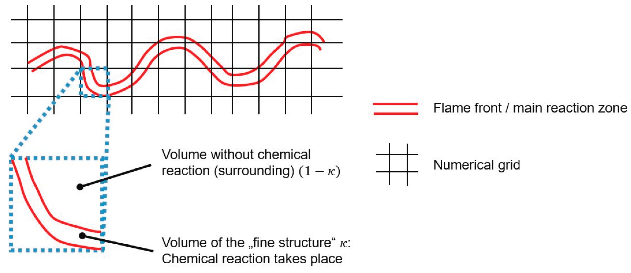
Figure 2.
Sketch of a wrinkled flame front and the modelling approaches using the plug flow reactor (PFR) and the perfectly stirred reactor (PSR) [45].
Figure 2.
Sketch of a wrinkled flame front and the modelling approaches using the plug flow reactor (PFR) and the perfectly stirred reactor (PSR) [45].
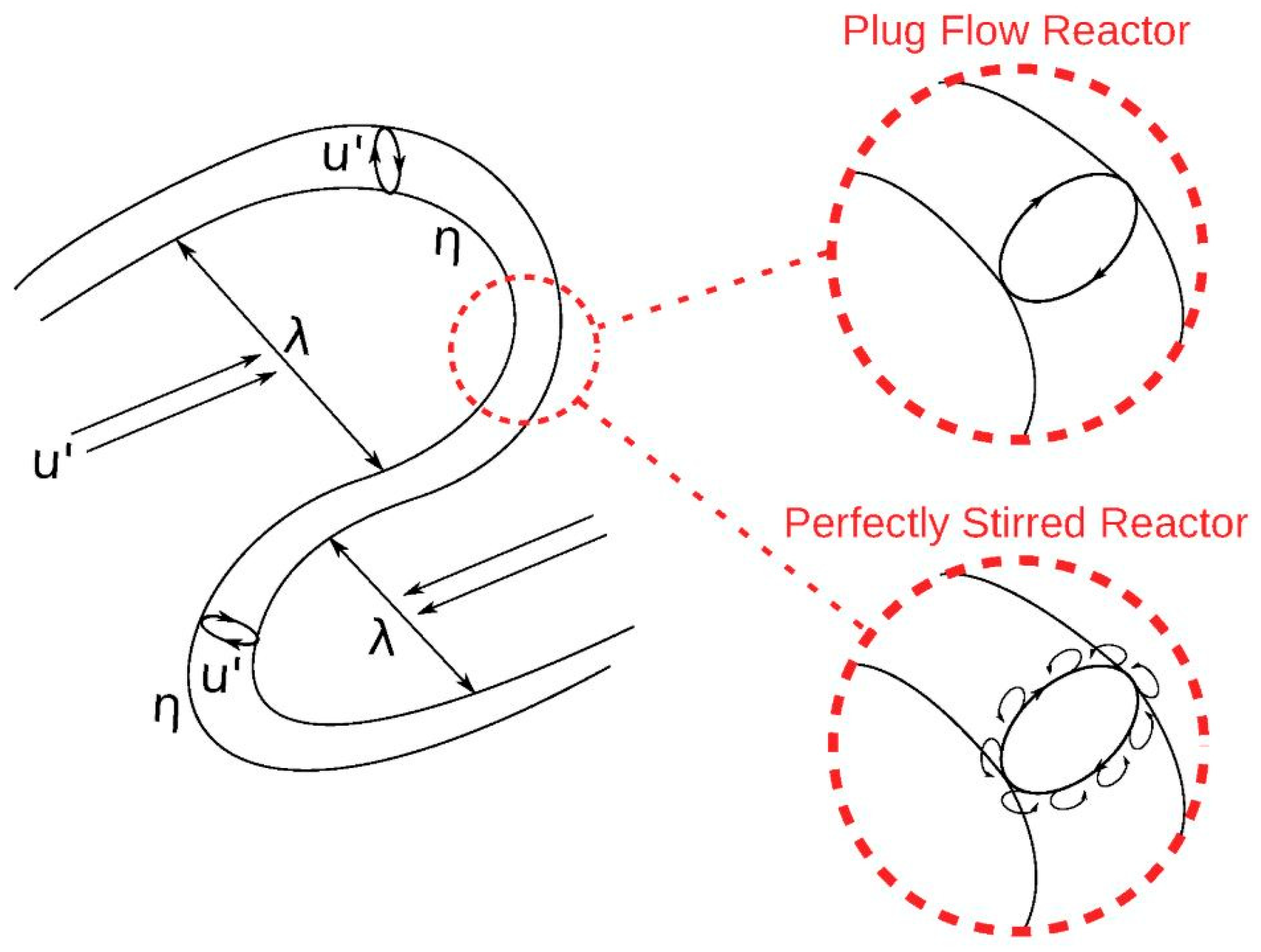
Figure 3.
Calculated mass fractions with Cantera for the combustion of a H2/O2 mixture in a PFR. Code used from [46].
Figure 3.
Calculated mass fractions with Cantera for the combustion of a H2/O2 mixture in a PFR. Code used from [46].
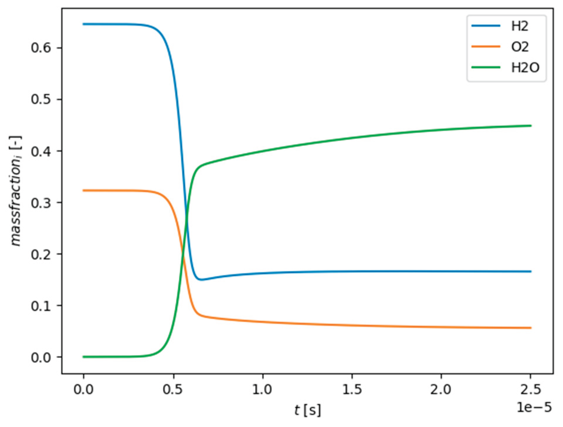
Figure 4.
Probability density function of the mass fraction of CH4 for the combustion case A_25/0_4100 (see section 4): Without Box-Cox transformation (left) and with Box-Cox transformation (right).
Figure 4.
Probability density function of the mass fraction of CH4 for the combustion case A_25/0_4100 (see section 4): Without Box-Cox transformation (left) and with Box-Cox transformation (right).
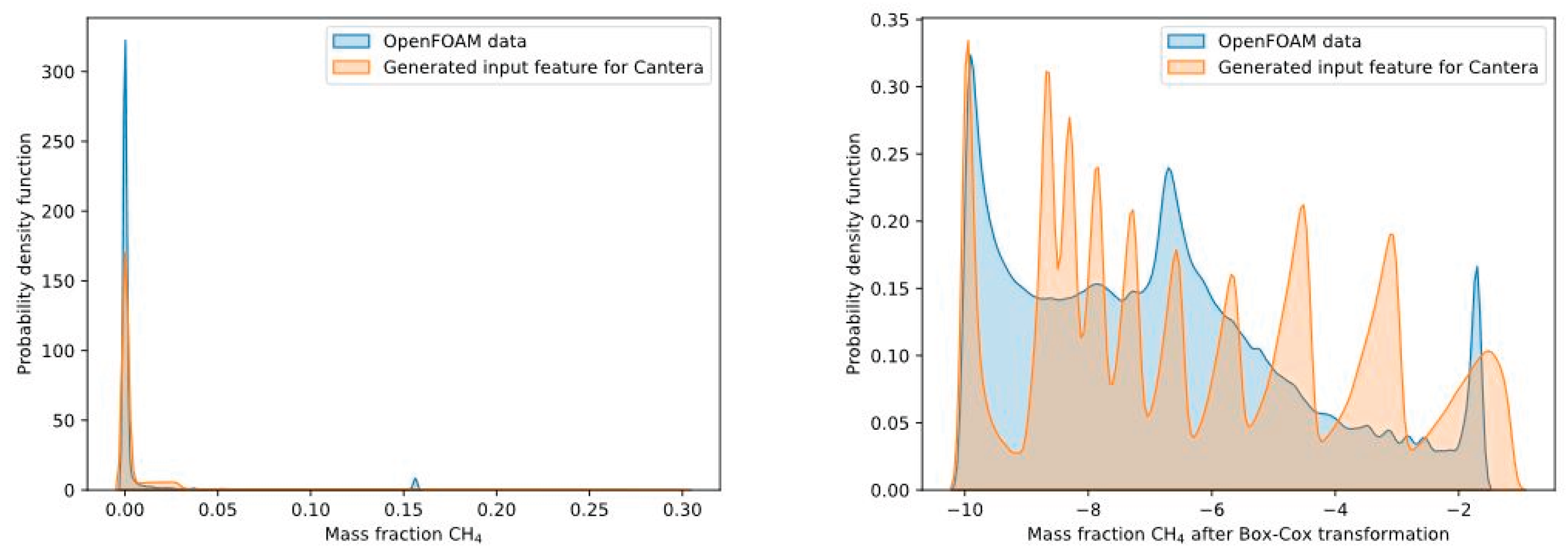
Figure 5.
Reaction rate of CH4 (left) and H2 (right) depending on the time scale for the combustion of CH4 (left) and H2 (right) with air and a Reynolds number of 4,100 in the main jet (combustion cases A_25/0_4100 and A_0/25_4100).
Figure 5.
Reaction rate of CH4 (left) and H2 (right) depending on the time scale for the combustion of CH4 (left) and H2 (right) with air and a Reynolds number of 4,100 in the main jet (combustion cases A_25/0_4100 and A_0/25_4100).
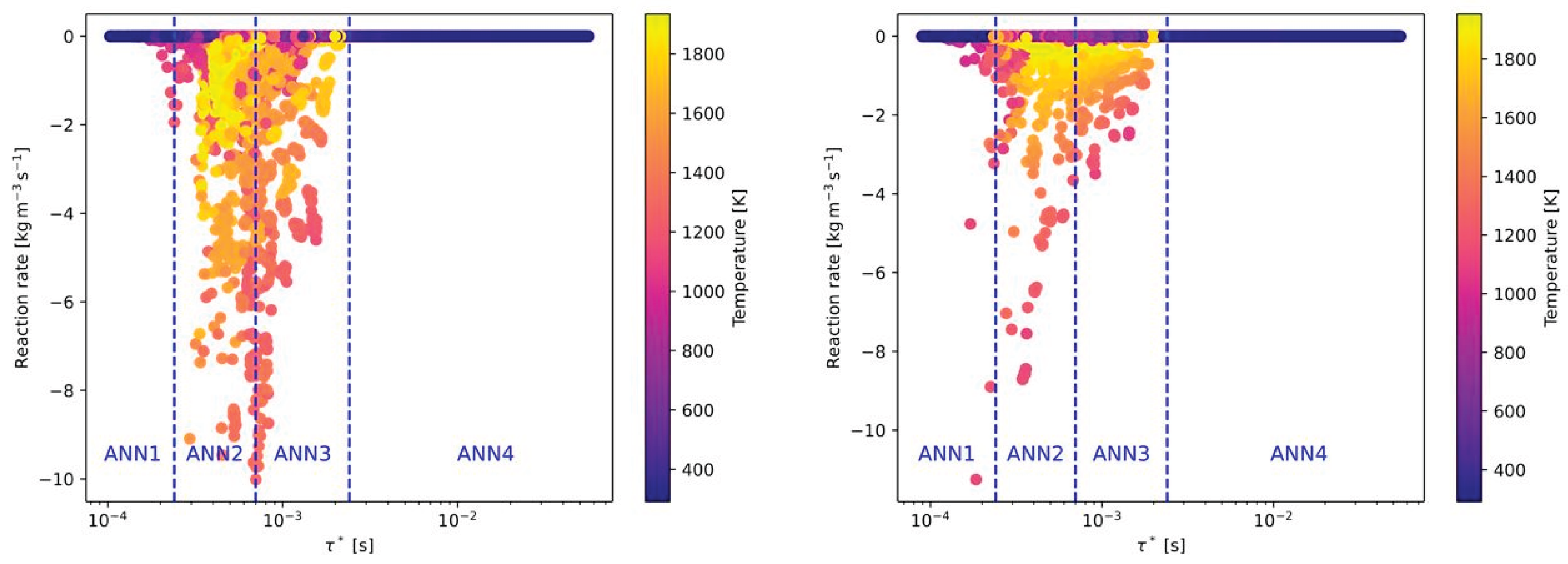
Figure 6.
Reaction rate of CH4 (left) and H2 (right) depending on the time scale for the combustion of CH4 (left) and H2 (right) with pure oxygen (oxy-fuel) and a Reynolds number of 4,100 in the main jet (combustion cases O_25/0_4100 and O_0/25_4100).
Figure 6.
Reaction rate of CH4 (left) and H2 (right) depending on the time scale for the combustion of CH4 (left) and H2 (right) with pure oxygen (oxy-fuel) and a Reynolds number of 4,100 in the main jet (combustion cases O_25/0_4100 and O_0/25_4100).
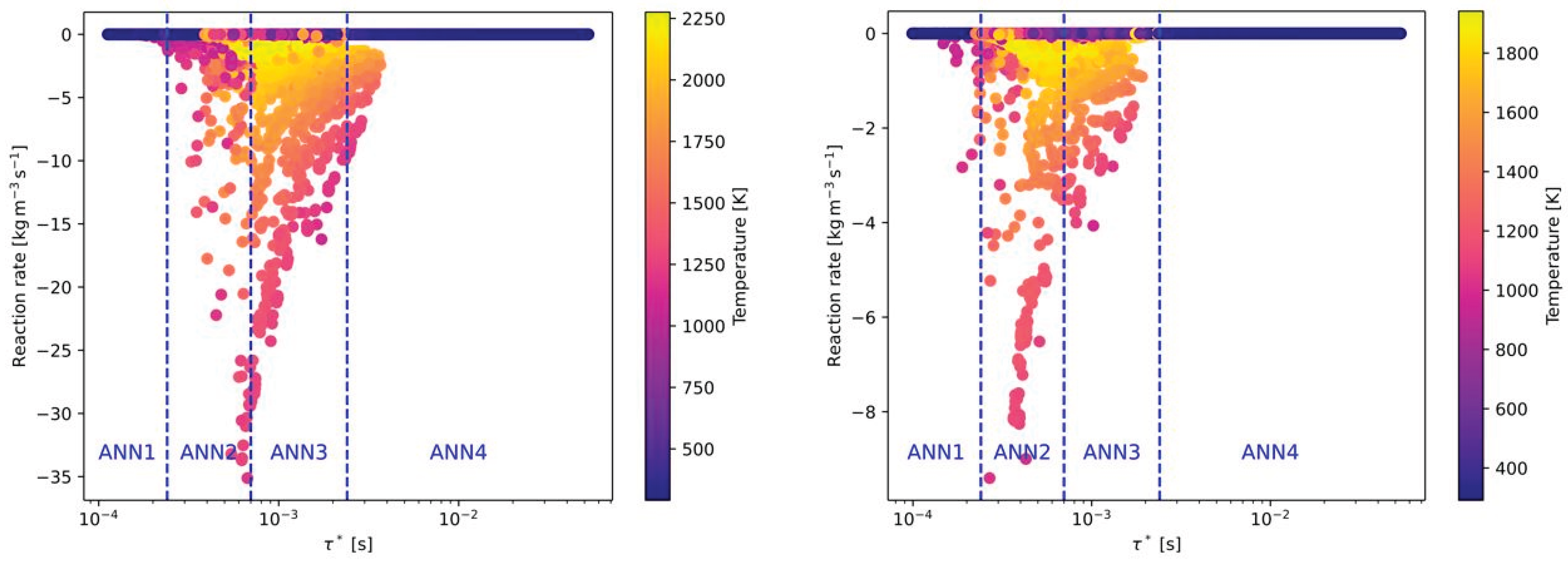
Figure 7.
Reaction rate of CH4 depending on the time scale for the combustion of CH4 with air (air-fuel) and a Reynolds number of 2,100 (left) and 12,400 (right) (combustion cases A_25/0_2100 and A_25/0_12400).
Figure 7.
Reaction rate of CH4 depending on the time scale for the combustion of CH4 with air (air-fuel) and a Reynolds number of 2,100 (left) and 12,400 (right) (combustion cases A_25/0_2100 and A_25/0_12400).
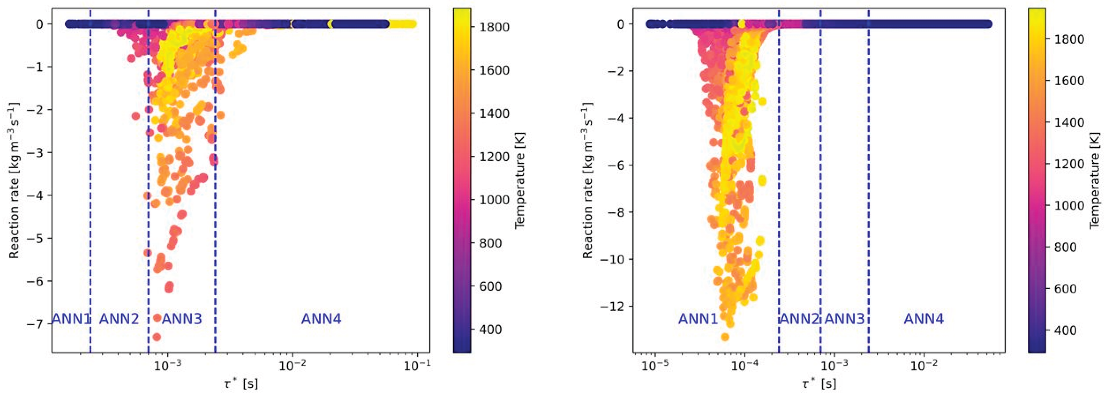
Figure 8.
Reaction rate of CH4 depending on the time scale for the combustion of CH4 with oxygen (oxy-fuel) and a Reynolds number of 2,100 (left) and 12,400 (right) (combustion cases O_25/0_2100 and O_25/0_12400).
Figure 8.
Reaction rate of CH4 depending on the time scale for the combustion of CH4 with oxygen (oxy-fuel) and a Reynolds number of 2,100 (left) and 12,400 (right) (combustion cases O_25/0_2100 and O_25/0_12400).
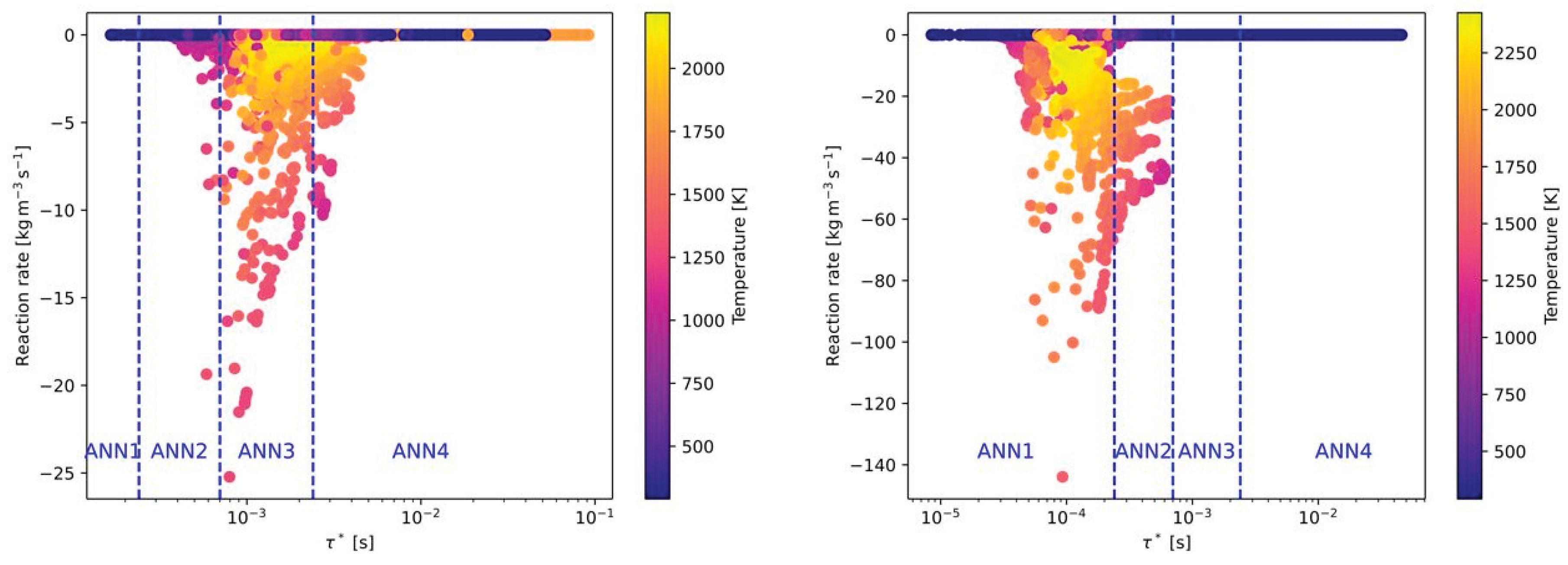
Figure 9.
Sketch of the burner setup to be investigated by OpenFOAM with the standard chemistry solver and the hybrid model (geometry based on the Sandia flame [59]).
Figure 9.
Sketch of the burner setup to be investigated by OpenFOAM with the standard chemistry solver and the hybrid model (geometry based on the Sandia flame [59]).
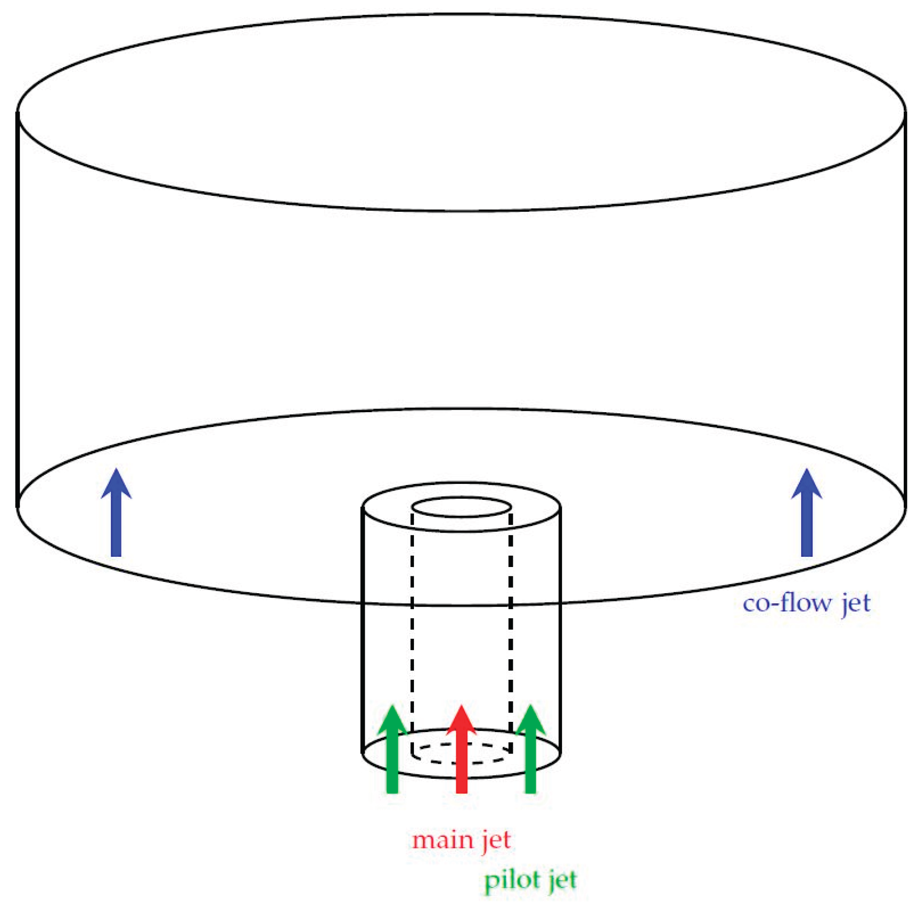
Figure 10.
Numerical grid.
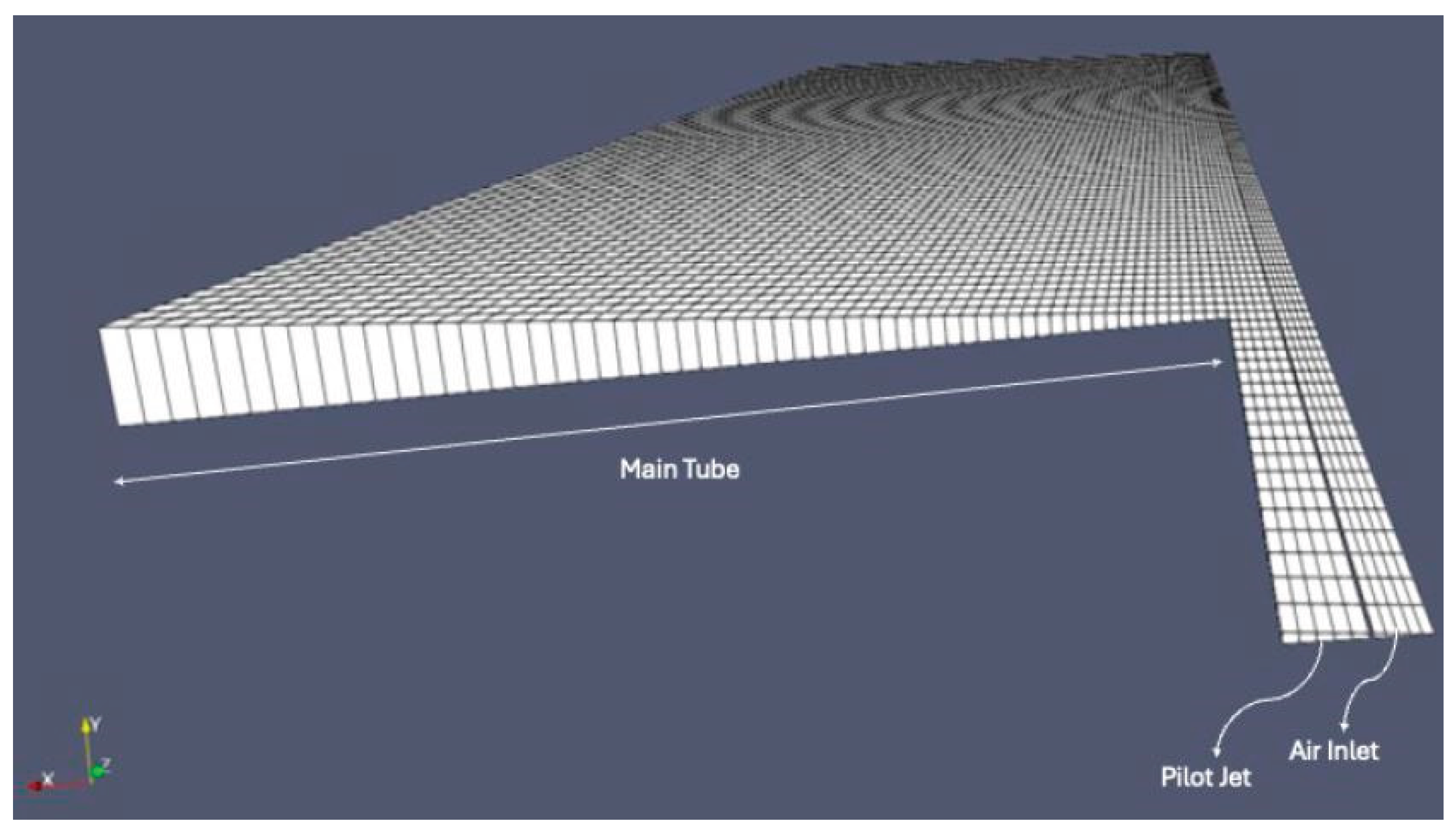
Figure 11.
Contour plots of the temperature for air-fuel combustion of 25 vol% (top), 10 vol% (middle) and 0 vol% (bottom) CH4 derived with ANNs to predict the chemistry (Reynolds number of 4,100).
Figure 11.
Contour plots of the temperature for air-fuel combustion of 25 vol% (top), 10 vol% (middle) and 0 vol% (bottom) CH4 derived with ANNs to predict the chemistry (Reynolds number of 4,100).
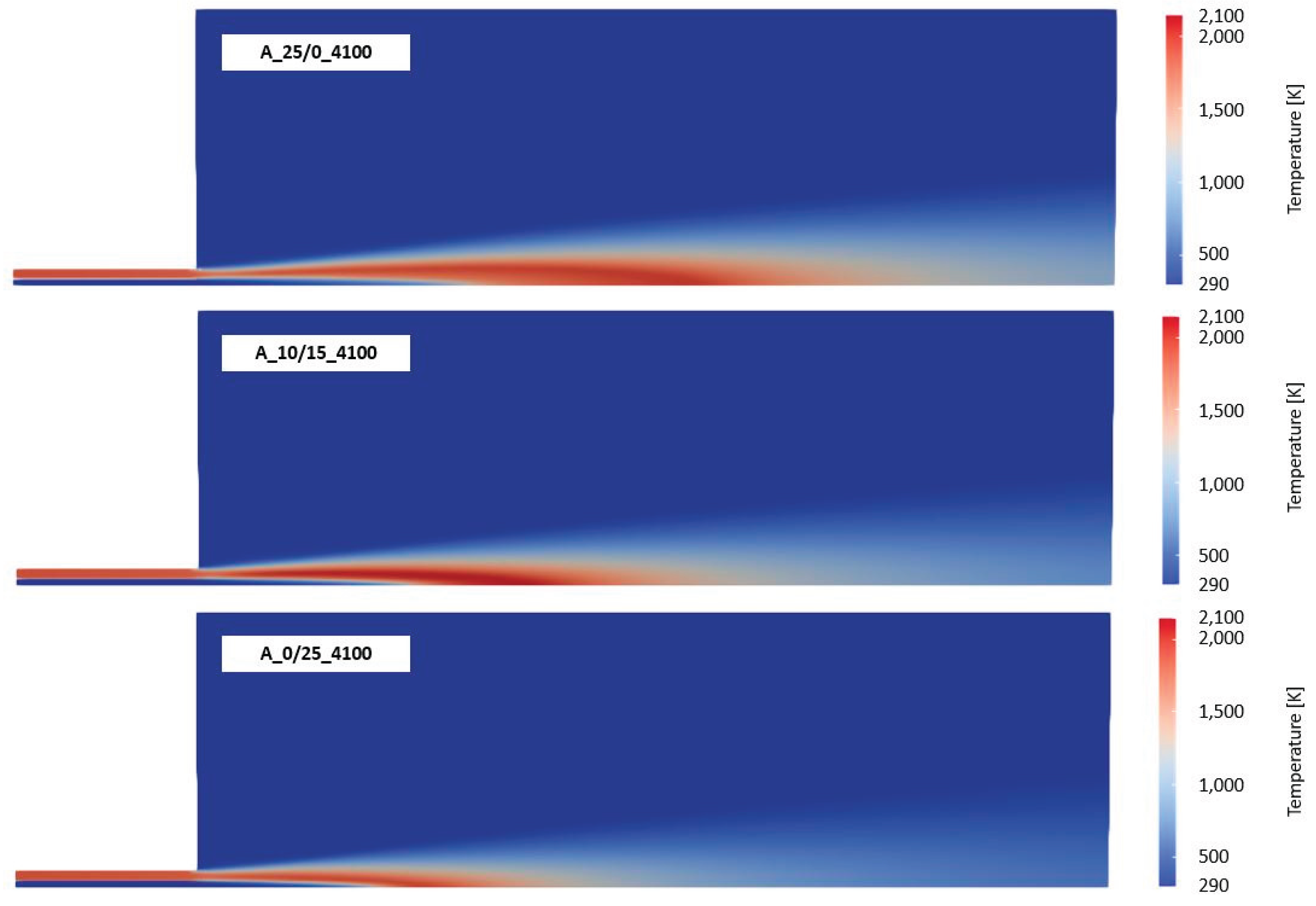
Figure 12.
Temperature along the center line of the burner for air-fuel combustion with different fuel compositions derived with the SC and ANNs (Reynolds number of 4,100).
Figure 12.
Temperature along the center line of the burner for air-fuel combustion with different fuel compositions derived with the SC and ANNs (Reynolds number of 4,100).
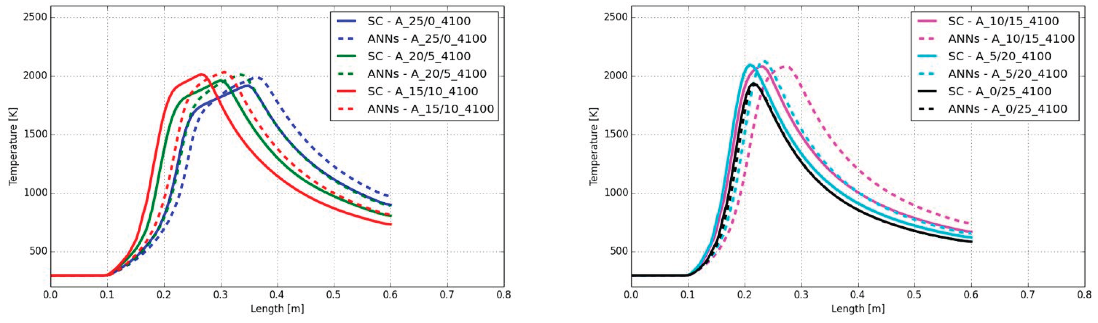
Figure 13.
CO mass fractions along the center line of the burner for air-fuel combustion with different fuel compositions derived with the SC and ANNs (Reynolds number of 4,100).
Figure 13.
CO mass fractions along the center line of the burner for air-fuel combustion with different fuel compositions derived with the SC and ANNs (Reynolds number of 4,100).
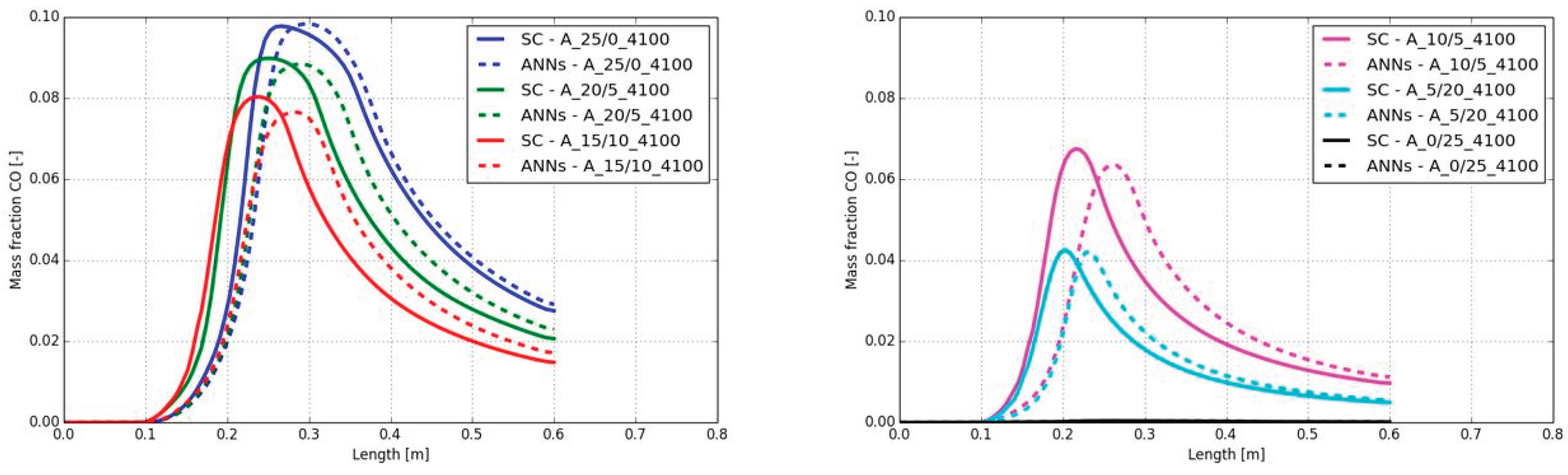
Figure 14.
Temperature along the center line of the burner for air-fuel combustion with 25 vol% CH4 and 0 vol% H2 derived with the SC and ANNs (Reynolds number of 4,100).
Figure 14.
Temperature along the center line of the burner for air-fuel combustion with 25 vol% CH4 and 0 vol% H2 derived with the SC and ANNs (Reynolds number of 4,100).
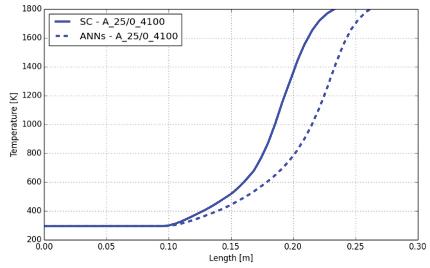
Figure 15.
Contour plots of the temperature for oxy-fuel combustion of 25 vol% (top), 10 vol% (middle) and 0 vol% (bottom) CH4 derived with ANNs to predict the chemistry (Reynolds number of 4,100).
Figure 15.
Contour plots of the temperature for oxy-fuel combustion of 25 vol% (top), 10 vol% (middle) and 0 vol% (bottom) CH4 derived with ANNs to predict the chemistry (Reynolds number of 4,100).
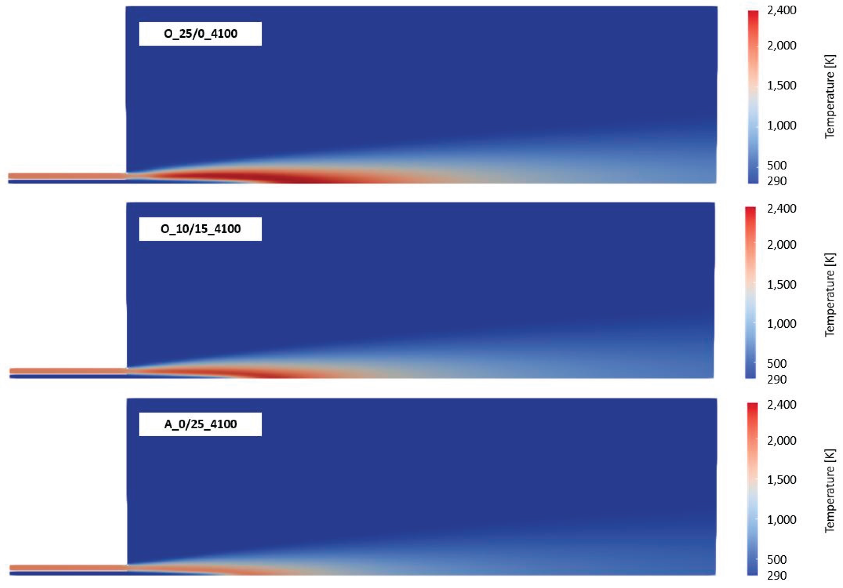
Figure 16.
Temperature along the center line of the burner for oxy-fuel combustion with different fuel compositions derived with the SC and ANNs (Reynolds number of 4,100).
Figure 16.
Temperature along the center line of the burner for oxy-fuel combustion with different fuel compositions derived with the SC and ANNs (Reynolds number of 4,100).
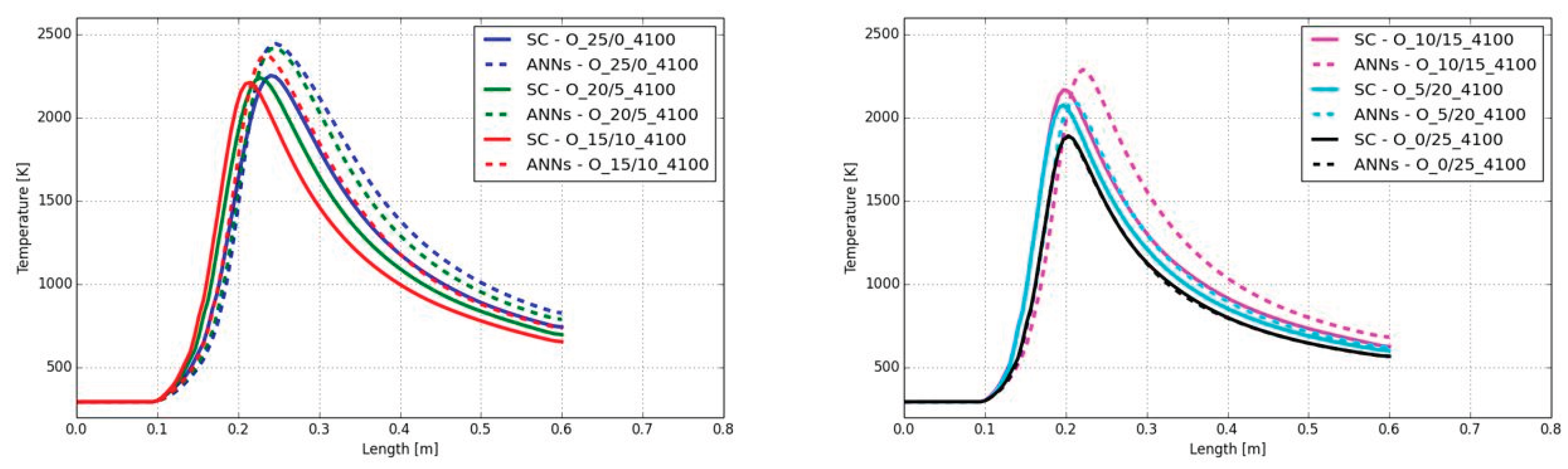
Figure 17.
CO mass fractions along the center line of the burner for oxy-fuel combustion with different fuel compositions derived with the SC and ANNs (Reynolds number of 4,100).
Figure 17.
CO mass fractions along the center line of the burner for oxy-fuel combustion with different fuel compositions derived with the SC and ANNs (Reynolds number of 4,100).
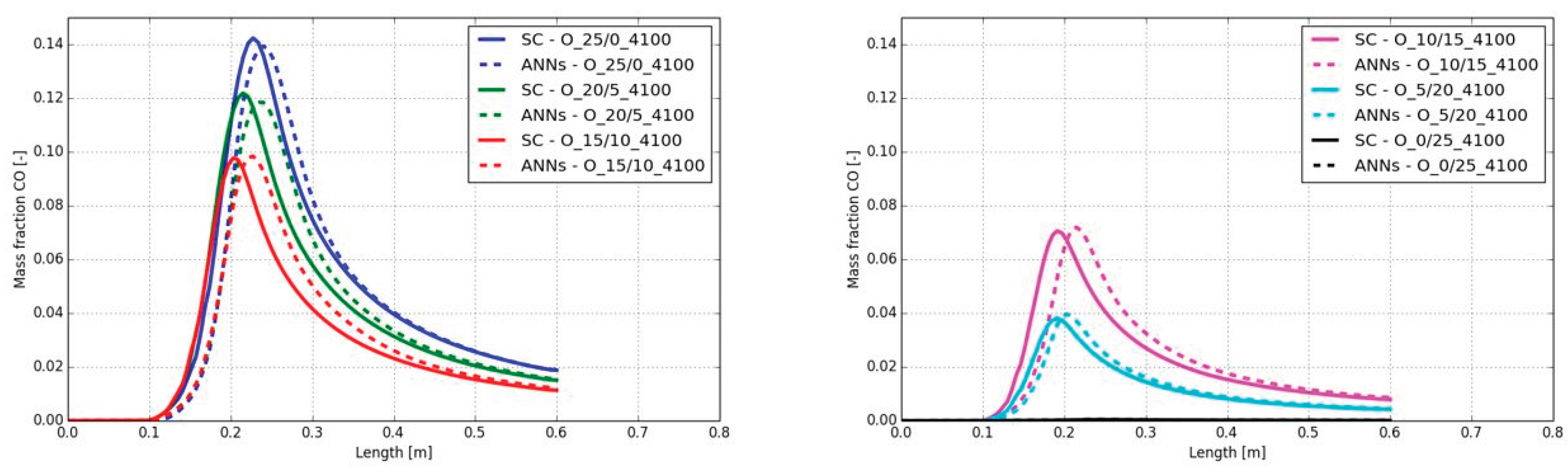
Figure 18.
Contour plots of the temperature for air-fuel combustion with Reynolds numbers of 2,100 (top), 8,300 (middle) and 12,400 (bottom) derived with ANNs to predict the chemistry (25 vol% CH4, 0 vol% H2).
Figure 18.
Contour plots of the temperature for air-fuel combustion with Reynolds numbers of 2,100 (top), 8,300 (middle) and 12,400 (bottom) derived with ANNs to predict the chemistry (25 vol% CH4, 0 vol% H2).
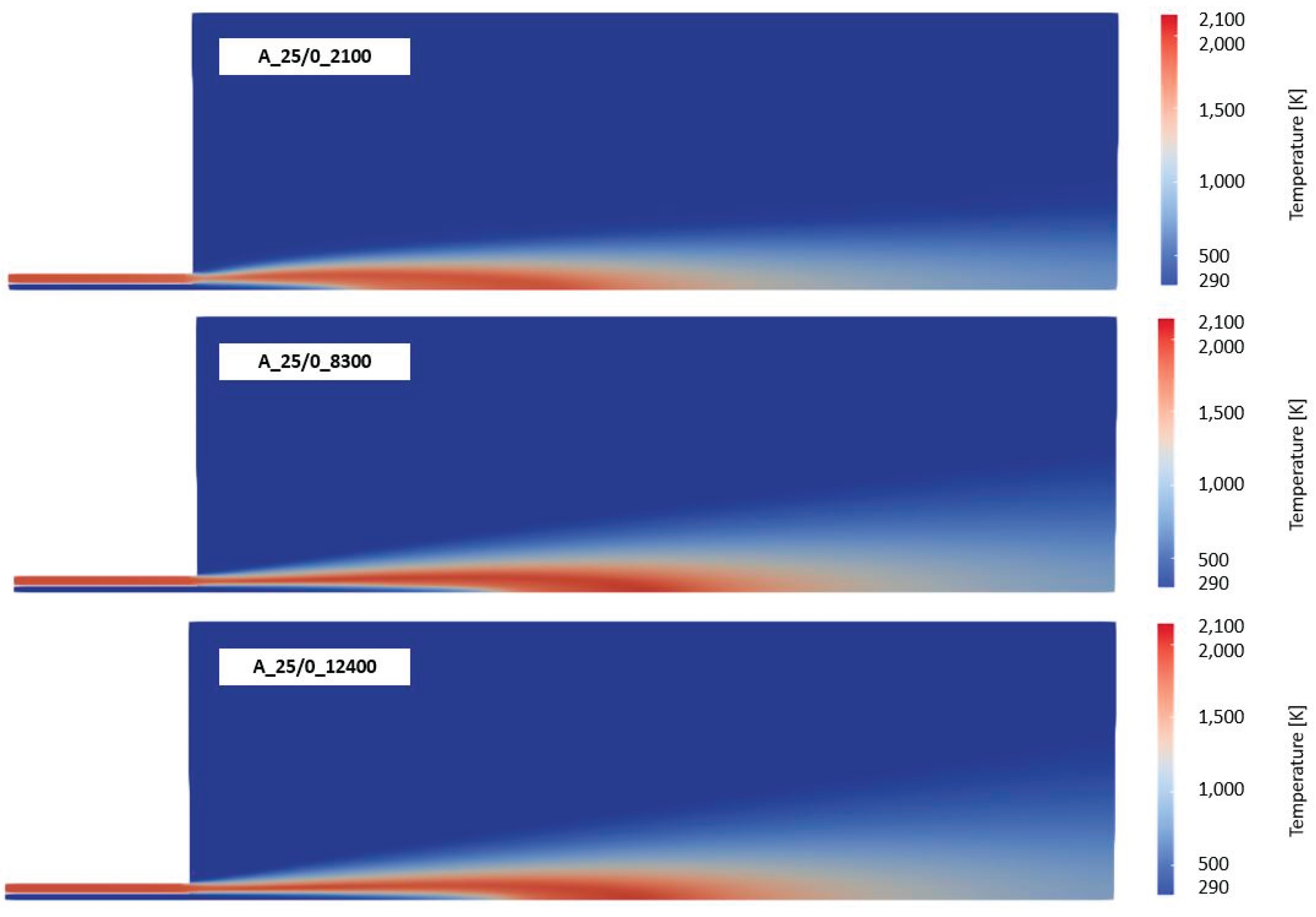
Figure 19.
Temperature along the center line of the burner for air-fuel combustion with different Reynolds numbers derived with the SC and ANNs (25 vol% CH4, 0 vol% H2).
Figure 19.
Temperature along the center line of the burner for air-fuel combustion with different Reynolds numbers derived with the SC and ANNs (25 vol% CH4, 0 vol% H2).
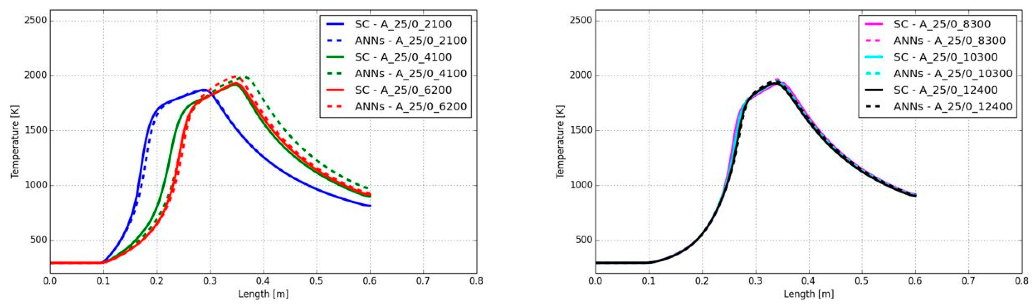
Figure 20.
CO mass fractions along the center line of the burner for air-fuel combustion with different Reynolds numbers derived with the SC and ANNs (25 vol% CH4, 0 vol% H2).
Figure 20.
CO mass fractions along the center line of the burner for air-fuel combustion with different Reynolds numbers derived with the SC and ANNs (25 vol% CH4, 0 vol% H2).
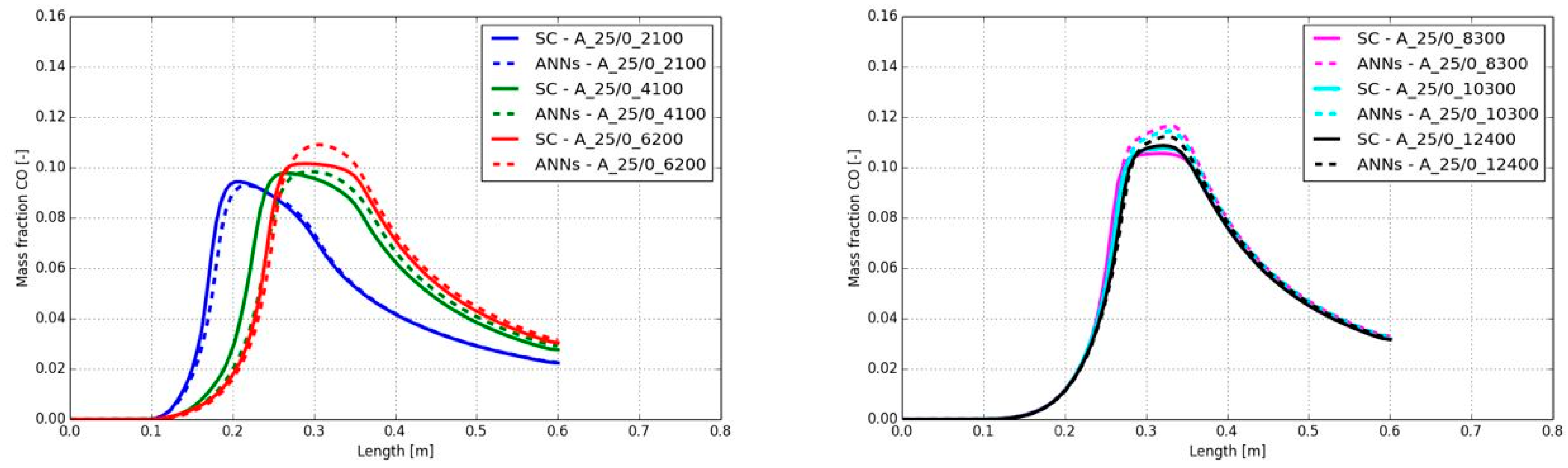
Figure 21.
Contour plots of the temperature for oxy-fuel combustion with Reynolds numbers of 2,100 (top), 8,300 (middle) and 12,400 (bottom) derived with ANNs to predict the chemistry (25 vol% CH4, 0 vol% H2).
Figure 21.
Contour plots of the temperature for oxy-fuel combustion with Reynolds numbers of 2,100 (top), 8,300 (middle) and 12,400 (bottom) derived with ANNs to predict the chemistry (25 vol% CH4, 0 vol% H2).
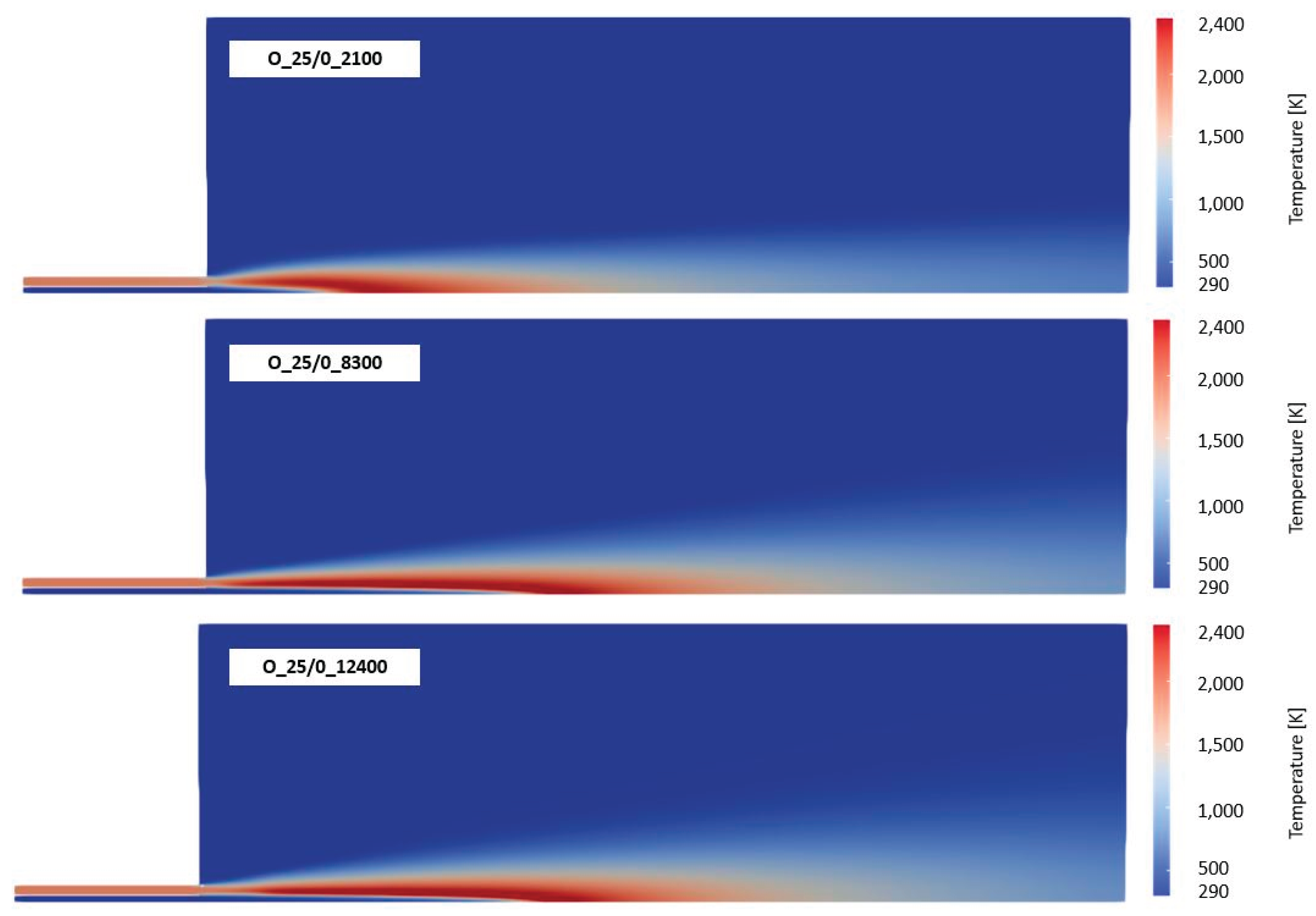
Figure 22.
Temperature along the center line of the burner for oxy-fuel combustion with different Reynolds numbers derived with the SC and ANNs (25 vol% CH4, 0 vol% H2).
Figure 22.
Temperature along the center line of the burner for oxy-fuel combustion with different Reynolds numbers derived with the SC and ANNs (25 vol% CH4, 0 vol% H2).
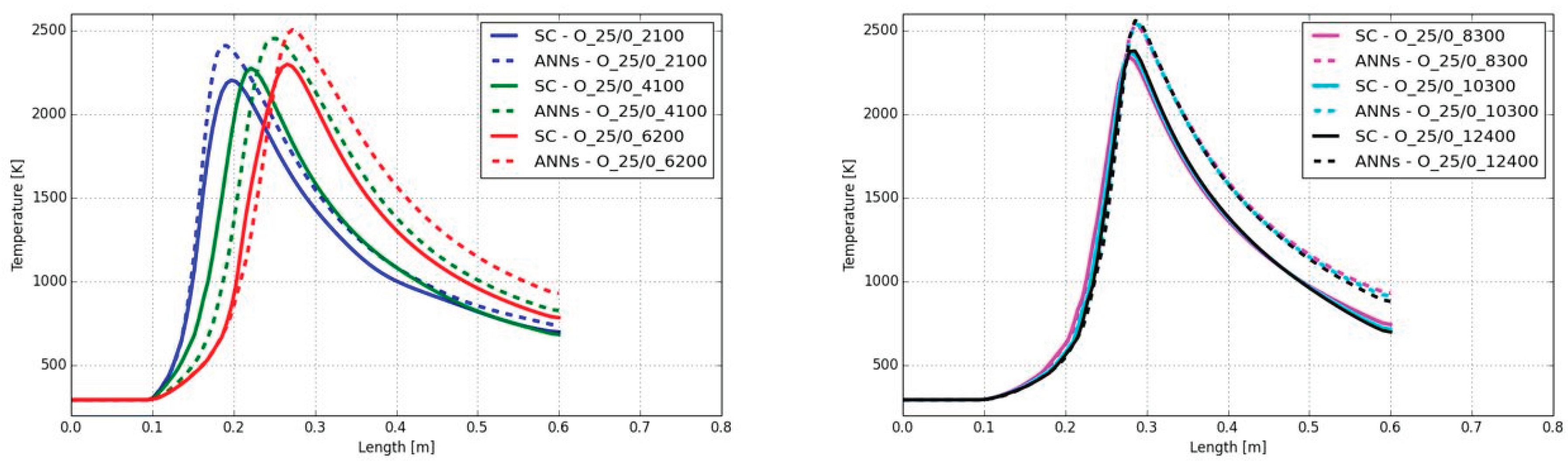
Figure 23.
CO mass fractions along the center line of the burner for oxy-fuel combustion with different Reynolds numbers derived with the SC and ANNs (25 vol% CH4, 0 vol% H2).
Figure 23.
CO mass fractions along the center line of the burner for oxy-fuel combustion with different Reynolds numbers derived with the SC and ANNs (25 vol% CH4, 0 vol% H2).
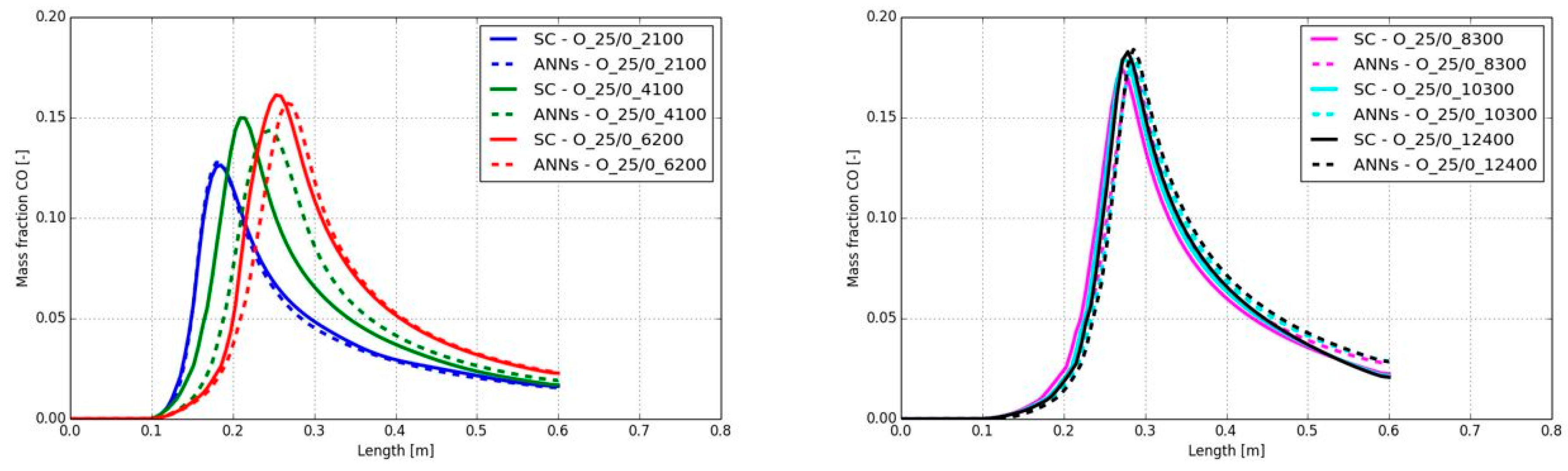
Figure 24.
Suggested ranges for the ANNs to increase the prediction accuracy in the low temperature region in a future work.
Figure 24.
Suggested ranges for the ANNs to increase the prediction accuracy in the low temperature region in a future work.
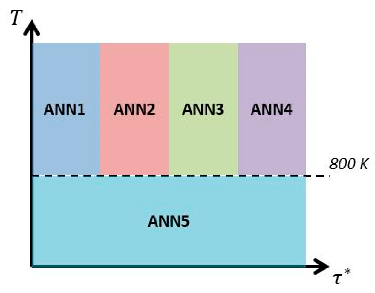

Table 1.
Reactions and Arrhenius parameters according to [44]. Units cal, mol, l, s.
Table 1.
Reactions and Arrhenius parameters according to [44]. Units cal, mol, l, s.
| Reaction | ||||
|---|---|---|---|---|
| 1 | ||||
| 2 | ||||
| 3 | ||||
| 4 | ||||
| 5 | ||||
| 6 |
Table 2.
Range of the input features and distribution during Monte Carlo sampling for data generation with Cantera (based on Reiter [47]).
Table 2.
Range of the input features and distribution during Monte Carlo sampling for data generation with Cantera (based on Reiter [47]).
| Feature | Minimum | Maximum | Distribution of sampling |
|---|---|---|---|
| [s] | 0 | 0.1 | Logarithmic |
| [K] | 250 | 2,600 | Homogenous |
| [-] | 0.0 | 1.0 | Homogenous |
| [-] | 0.0 | 0.3 | l |
| [-] | 0.0 | 0.3 | l |
| [-] | 0.0 | 0.3 | l |
| [-] | 0.0 | 0.3 | l |
| [-] | 0.0 | 0.8 | - |
| [-] | 0.0 | 0.3 | l |
| [-] | 0.0 | 0.005 | s |
| [-] | 0.0 | 0.005 | s |
| [-] | 0.0 | 0.3 | l |
Table 3.
Mass fractions and their corresponding possibility in the Monte Carlo sampling (based on Früh [49]).
Table 3.
Mass fractions and their corresponding possibility in the Monte Carlo sampling (based on Früh [49]).
| Probability [s] | Probability [l] | |
|---|---|---|
| 0.0 – 10-30 | 0.0005 | 0.0005 |
| 10-29 – 10-10 | 0.005 | 0.005 |
| 10-9 – 10-5 | 0.08 | 0.08 |
| 10-4 | 0.2425 | 0.08 |
| 10-3 | 0.2425 | 0.135 |
| 10-2 – 10-1 | 0.0 | 0.135 |
Table 4.
ANN and their corresponding ranges for the fine structures time scales.
| ANN | [s] | [s] |
|---|---|---|
| 1 | 0 | 0.00024 |
| 2 | 0.00024 | 0.00055 |
| 3 | 0.00055 | 0.00117 |
| 4 | 0.00117 | 0.1 |
Table 5.
Errors during ANN training using different sizes for the data set.
| Size of data set | MAE | MSE | RMSE |
|---|---|---|---|
| 2 | 0.097 | 1.018 | 0.346 |
| 4 | 0.082 | 0.912 | 0.288 |
| 8 | 0.059 | 0.478 | 0.221 |
| 16 | 0.055 | 0.345 | 0.196 |
| 32 | 0.051 | 0.333 | 0.191 |
Table 6.
Operating conditions of the flame in basis configuration.
| Main jet | Pilot jet | Co-flow | ||
|---|---|---|---|---|
| Temperature [K] | 294 | 1880 | 291 | |
| Velocity [m/s] | 10.0 | 5.0 | 0.9 | |
| Volume fraction [%] |
25 | 0 | 0 | |
| 0 | 0.40 | 0 | ||
| 0 | 6.92 | 0 | ||
| 0 | 0.07 | 0 | ||
| 0 | 0.18 | 0 | ||
| 0 | 14.50 | 0 | ||
| 58 | 72.66 | 0.79 | ||
| 0 | 0.13 | 0 | ||
| 17 | 4.68 | 21 | ||
| 0 | 0.46 | 0 | ||
Table 7.
Volume fraction of nitrogen and oxygen for air-fuel and oxy-fuel conditions.
| Main jet | Co-flow | ||||
|---|---|---|---|---|---|
| Air-fuel | Oxy-fuel | Air-fuel | Oxy-fuel | ||
| Volume fraction [%] | 17 | 75 | 21 | 100 | |
| 58 | 0 | 79 | 0 | ||
Table 8.
Velocities at the burner inlets for the different fuel mixtures under air-fuel conditions in [m/s].
Table 8.
Velocities at the burner inlets for the different fuel mixtures under air-fuel conditions in [m/s].
| Vol. frac. ratio |
25/0 | 20/5 | 15/10 | 10/15 | 5/20 | 0/25 |
|---|---|---|---|---|---|---|
| Main jet | 10.0 | 10.3 | 10.5 | 10.8 | 11.1 | 11.5 |
| Pilot jet | 5.0 | 5.0 | 5.0 | 5.0 | 5.0 | 5.0 |
| Co-flow | 0.9 | 0.9 | 0.9 | 0.9 | 0.9 | 0.9 |
Table 9.
Velocities at the burner inlets for the different fuel mixtures under oxy-fuel conditions in [m/s].
Table 9.
Velocities at the burner inlets for the different fuel mixtures under oxy-fuel conditions in [m/s].
| Vol. frac. ratio | 25/0 | 20/5 | 15/10 | 10/15 | 5/20 | 0/25 |
|---|---|---|---|---|---|---|
| Main jet | 9.2 | 9.4 | 9.6 | 9.8 | 10.1 | 10.4 |
| Pilot jet | 5.0 | 5.0 | 5.0 | 5.0 | 5.0 | 5.0 |
| Co-flow | 0.9 | 0.9 | 0.9 | 0.9 | 0.9 | 0.9 |
Table 10.
Velocities at the burner inlets for the different turbulence levels under oxy-fuel conditions in [m/s].
Table 10.
Velocities at the burner inlets for the different turbulence levels under oxy-fuel conditions in [m/s].
| Reynolds number | Main jet | Pilot jet | Co-flow |
|---|---|---|---|
| 2,100 | 5.0 | 2.5 | 0.9 |
| 4,100 (basis) | 10.0 | 5.0 | 0.9 |
| 6,200 | 15.0 | 7.5 | 0.9 |
| 8,300 | 20.0 | 10.0 | 0.9 |
| 10,300 | 25.0 | 12.0 | 0.9 |
| 12,400 | 30.0 | 15.0 | 0.9 |
Disclaimer/Publisher’s Note: The statements, opinions and data contained in all publications are solely those of the individual author(s) and contributor(s) and not of MDPI and/or the editor(s). MDPI and/or the editor(s) disclaim responsibility for any injury to people or property resulting from any ideas, methods, instructions or products referred to in the content. |
© 2025 by the authors. Licensee MDPI, Basel, Switzerland. This article is an open access article distributed under the terms and conditions of the Creative Commons Attribution (CC BY) license (http://creativecommons.org/licenses/by/4.0/).
Copyright: This open access article is published under a Creative Commons CC BY 4.0 license, which permit the free download, distribution, and reuse, provided that the author and preprint are cited in any reuse.


