Submitted:
03 June 2025
Posted:
04 June 2025
You are already at the latest version
Abstract
Some cities are characterized by knowledge spillover industries, which drive innovation, entrepreneurship, and growth nationwide. Urbanization brings the accumulation of material resources, and the emergence of these “knowledge-spillover” cities relies on sufficient labor force inflows. However, the excessive expansion of megacities overabsorbs labor from other cities, reducing the number of “knowledge-spillover” cities and national innovation potential. Analysis of China’s employment population structure indicates that “knowledge-spillover” cities need to be based on a population of 10 million. Currently, the unchecked expansion of individual megacities not only causes metropolitan malaise and regional imbalance but also limits the emergence of new “knowledge-spillover” cities, which is unfavorable for economic development. We suggest that China need pay more attention to the construction of urban agglomerations as a geographic or administrative unit.
Keywords:
revealed comparative advantage
; urban scale
; knowledge spillover
; employment structure
; innovative development
1. Introduction
The emergence of cities is a symbol of the maturity and civilization of human beings [1,2]. Inevitable urbanization processes bring the accumulation of various material resources, such as capital, materials, commodities, and labor. The concentration and proper distribution of resources reduce various production and living costs, improve the social efficiency of the city, and promote the further concentration and distribution of material resources. With the development of the economy and technological progress, more emerging industries and employment opportunities appear in cities. This directly leads to the rapid expansion of urban size [3] and the complexity of economic activities [4].
The growth of the urban population is not random but follows a structured pattern [5]. According to studies, different industries have varying contributions to urban economic growth and exhibit different employment growth rates [6,7]. In urban scaling theory, the relationship between employment in different industries and urban population is often described by the power-law function [8,9], where N represents the population of the city, and represents the employment in industry i. Industries that exhibit superlinear growth in employment relative to urban population () are generally considered to be driven by “knowledge spillovers”, whereas urban infrastructure industries () show the opposite trend [8,10]. This suggests that the dependencies of population during urbanization may underpin the urban economic structure and promote its evolution [5], as the output and employment share of knowledge spillover industries continue to increase compared to infrastructure industries [11,12]. The employment structure of metropolitan regions has evolved in the post-industrialization era [13,14,15]. In cities where the production advantages in “knowledge-spillover” industries (with ) are more pronounced, these cities are referred to as “knowledge-spillover” cities. Some scholars argue that the emergence of “knowledge-spillover” cities is contingent upon a sufficiently large population. The most recent quantitative analyses indicate that in the United States, “knowledge-spillover” cities only begin to emerge when the population exceeds 1.2 million [7].
China’s large population and abundant regional labor flows [16] provide a strong basis for rapid urbanization [17,18] and the construction of several international metropolises [19,20]. Meanwhile, China’s urbanization process has also exhibited patterns of shifting from manufacturing to service industries, as well as the gradual emergence of knowledge-spillover industries as key drivers of urban growth. However, some megacities, even with populations exceeding those of major international metropolises in developed countries, still have dominant industries that are basic in nature and contribute limited value to GDP growth. This situation has sparked debates among scholars regarding whether China should restrict the size of its super-large cities [21,22]. The emergence of “knowledge-spillover” cities, which are expected to drive economic innovation and sustainable growth, has been hindered. This issue is characterized by the excessive expansion of a few megacities, which not only leads to “metropolitan malaise” and unbalanced regional development but also limits the emergence of other “knowledge-spillover” cities [5,23]. Addressing this issue requires an analysis of the co-evolutionary patterns between urban population size and industrial structure transformation.
This research aims to examine the mechanism by which population distribution characteristics promote urban evolution in China, with a focus on the emergence of “knowledge-spillover” cities. Specifically, it explores how urban population distribution affects urban evolution and identifies the labor conditions required for the emergence of “knowledge-spillover” cities. It demonstrates that the longitudinal change of urban economies indeed follows a universal process governed by changes in population size. The objectives of this study are to understand the underlying mechanisms driving urban development and to provide insights into fostering a more balanced and sustainable urbanization process in China. It also seeks to identify the population thresholds and labor conditions necessary for the emergence of knowledge-spillover cities.
2. Literature Review
The labor force and contributing individuals, who each represent a producer, a consumer, and a member of society in the urban area, are the most fundamental resource for any urban area. Generally, the distribution of population among urban areas is uneven, where N is the urban population and is the distribution function. Empirical data confirm that urban populations typically follow a Pareto distribution [24,25], Zipf’s law 1, or a log-normal distribution [26,27,28]. These distributions all feature a negative exponent of N, suggesting that population concentration results in a few large metropolises standing out from many smaller urban areas [29,30]. However, significant differences in the quality of urbanization and industrial structure exist among urban areas of varying sizes [5]. According to Zhao (2017), the shift from the manufacturing industry to the service industry as the leading economic sector is an important reason for the continuous growth of urban areas [31]. But not all expanding urban areas can leverage “knowledge spillovers” to become centers of superlinear growth industries and thus gain competitive advantages. Therefore, understanding how the distribution characteristics of urban populations influence the evolution of urban areas and how urban expansion can be effectively managed to better support the economic structure and foster “knowledge-spillover” urban areas are questions of great interest to scholars and policymakers.
Scholars have already explored the general patterns by which increasing urban population sizes drive structural transformations in urban areas. Friedmann (2006) points out that the disparity in urban size leads to great inconsistency between the quality of spatial development in urbanization and the quality of social development [32]. According to Frank and Balland (2018, 2020), small urban areas heavily rely on manual labor, while large urban areas rely on cognitive labor [4,33]. They suggest that as the urban population increases, there is a transformation of industries from labor-intensive to capital-intensive and knowledge-technology-intensive, or from agriculture-led to manufacturing-led and modern services-led [11]. Recent quantitative analyses in the United States show that “knowledge-spillover” urban areas emerge only when the population exceeds 1.2 million [7].
China’s early rapid urbanization process [34,35] and subsequent “polarization” problem [36,37,38] have inspired comprehensive analyses of the mechanisms by which population promotes urban evolution. China’s large population base and substantial migrant population have enabled the rapid formation of multiple international metropolises. During 2020–2021, China had 21 urban areas with populations exceeding 5 million [39] and 17 urban areas with populations exceeding 10 million [40]. However, the emergence of “knowledge-spillover” urban areas has not been sufficient. Therefore, it is necessary to investigate whether similar general patterns exist in China, where population size drives urban transformation, and to identify the population threshold for such transformations. Our research demonstrates that the longitudinal change of urban economies indeed follows a universal process governed by changes in population size.
In summary, while significant progress has been made in understanding the relationship between urban population dynamics and economic evolution, gaps remain in identifying the specific mechanisms and thresholds that drive the emergence of knowledge-spillover urban areas. Future research should focus on bridging these gaps, particularly in the context of China’s unique urbanization trajectory. The remainder of this study is arranged as follows: Section 3 introduces the data source and methods; Section 4 describes the scaling characteristics of employment in different industries and indicates that urban areas have different comparative advantages, which is the basic assumption to discuss urban development and innovation; and analyzes the evolution of knowledge spillover industries and illustrates the labor demand and its limitations for “knowledge-spillover” urban areas in China. Section 5 provides the conclusion and discussion.
3. Data & Methods
3.1. Data Source and Preprocessing
The dataset encompasses the urban population of prefecture-level and higher cities in China, along with their employment across various industries. Given the substantial floating population in China, studies on urban evolution typically utilize resident population data2. The resident population accurately reflects the mobility characteristics of the current Chinese population and provides a precise depiction of urbanization levels based on resident population standards. For instance, China’s census data are based on the resident population.
3.1.1. Resident Population Data for Cities During 2004-2019
In January 2004, the National Bureau of Statistics mandated that all provinces, autonomous regions, and municipalities calculate Gross Regional Product (GRP) per capita using resident population data.3 Due to the lack of publicly available and reliable resident population data, the urban population of each city was estimated using the formula from 2004 onwards. The effectiveness of this estimation method is discussed. A reliability analysis of the estimated data for four typical cities is provided in Appendix A.1.2.
The GRP and GRP per capita data are sourced from the “China City Statistical Yearbook”. Since it ceased reporting industry-specific employment data for prefecture-level cities starting from 2020, the dataset is confined to the period up to 2019. To extend the dataset to 2020, data from the 7th National Population Census were incorporated. Given that the census is conducted decennially and that the employment population distribution in prefecture-level cities was significantly influenced in the short term by the COVID-19 pandemic in 2020, the supplementary data for 2020 are presented exclusively in Appendix A.2.1. There, the implications for the conditions under which “knowledge-spillover” cities emerge in 2020, given the altered characteristics of urban population distribution, are examined.
3.1.2. 280 Cities and 19 Industries
Since 2019, China has 4 municipalities and 293 prefecture-level cities. The employment data for 19 industries for the period 2004–2019 were selected from the “China City Statistical Yearbook”. The industries are defined according to the Industry Classification of the National Economy (GB/T 4754). However, employment data for certain industries were missing in some cities. Although these cases are few, they required rigorous preprocessing. Interpolation was employed for non-endpoint missing values, and regression prediction was used to interpolate endpoint vacancy values (details in Appendix A.2.2).
The detailed data are provided in Table 1. To ensure consistency in the statistical caliber, 18 cities those lacking a significant amount of data were excluded 4. The effective sample thus includes 276 prefecture-level cities and 4 municipalities directly under the central government, totaling 280 cities. Based on the classification of China’s four major economic regions (see Table A4 in the Appendix), there are 86 cities in the eastern region, 80 cities in the central region, 80 cities in the western region, and 34 cities in the northeast region.

Table 1.
Data description
| Variable | Variable Description | Data Source |
|---|---|---|
| Employment in China | The employment of 19 industries in prefecture-level and above cities, annual data during 2004-2019, from “China City Statistical Yearbook”, 10 thousands people. | https://data.cnki.net/yearBook/single?id=N2025020156&pinyinCode=YZGCA |
| GRP, GRP (per capita) in China | The gross regional product and gross regional product per capita in prefecture-level and above cities of China, the annual data during 2004-2012 and 2014-2019 are from “China City Statistical Yearbook”, and the annual data in 2013 is from “China Regional Economic Statistical Yearbook”, yuan. | https://data.cnki.net/yearBook/single?id=N2025020156&pinyinCode=YZGCA; https://data.cnki.net/yearBook/single?id=N2015070200&pinyinCode=YZXDR |
| Sales of commodities in China | Total retail sales of consumer goods + total sales of commodities of enterprises above designated size in wholesale and retail trades prefecture-level and above cities of China, annual data in 2019, from “China City Statistical Yearbook”, 10 000 yuan. | https://data.cnki.net/yearBook/single?id=N2025020156&pinyinCode=YZGCA |
| GDP (per capita) in the United States | CAGDP1 gross domestic product (GDP) summary by metropolitan area, from U.S. Bureau of Economic Analysis, annual data during 2004-2019, thousands of chained 2012 dollars. | https://www.bea.gov/data/gdp/gdp-county-metro-and-other-areas |
| Polulation in the United States | Annual estimates of the resident population for metropolitan statistical areas in the United States, from U.S. Census Bureau, Population Division, annual data in 2019, people. | https://www.census.gov/data/datasets/time-series/demo/popest/2010s-total-metro-and-micro-statistical-areas.html |
| Sales of commodities in the United States | Real personal consumption expenditures by States, real personal income by metropolitan area, annual data in 2019, from U.S. Bureau of Economic Analysis, millions of constant (2012) dollars. | https://www.bea.gov/sites/default/files/2021-12/rpp1221.xlsx |
3.2. The Comparative Advantage of Industries and Its Critical Point Analysis
For city c, the revealed comparative advantage () of industry i in all employment is quantified as [7,41,42]
where denotes the employment of industry i in city c. Specifically, an industry i is considered characteristic in city c if , while indicates a lack of specialization [7].
Some literature uses scaling exponents to explore the distribution of employment to reflect the technical level of industries [11,12]. Other scholars analyze the city’s growth model by examining the distribution of urban population using scaling exponents [43,44]. However, few studies consider urban population and employment together. Inho Hong et al. (2020) explored the relationships between urban size growth and urban innovation using the scaling exponent . They found that superlinearity () is typically associated with knowledge spillover industries, while sublinear scaling () is often attributed to infrastructure industries [7,10].
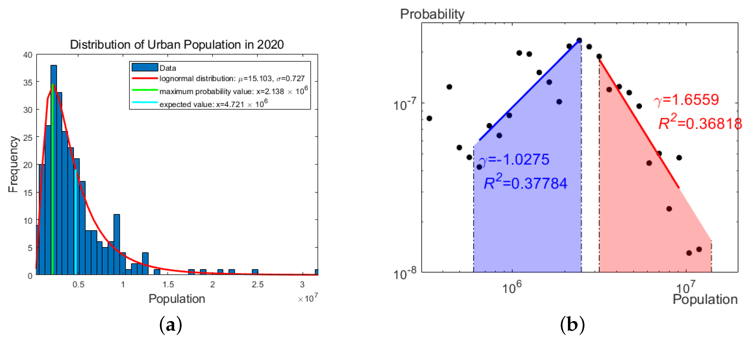
Although the power-law distribution is common in urban populations and other socioeconomic systems [45,46,47], not all countries or regions follow this pattern [48,49]. Some existing literature suggests that China’s urban population does not follow a power-law distribution [43] but rather obeys a log-normal distribution [50]. Here, based on the data of urban residents, it is verified that China’s urban population satisfies the log-normal distribution (see Figure A2 in the Appendix). In the range of relatively small or large N, it can be assumed that the distribution function is linear under double logarithmic coordinates, as in , where is the coefficient of the explanatory variable [42,51,52].
The function of comparative advantage is then derived as follows, with the details provided in Appendices Appendix B.1 and Appendix B.2:
According to Eq. 3, the change in with respect to the scaling exponent and population N is quantified. This allows for the analysis of the universal development path and labor demand of cities in China by comparing the evolution of employment advantage among industries.
In physics, a critical point of the function is a point in the function’s domain where it is either not holomorphic or the derivative is equal to zero [53]. On the surface of the graph of the function (a two-dimensional surface composed of and N), the critical point is defined by . This indicates that no matter how the two parameters change near this point, the value of will remain unchanged. Thus, it is defined as a fixed point in mathematics. Whether the critical point is stable depends on whether the point is a minimum or a maximum. For a one-dimensional function, the critical point is relatively easy to judge. For example, for the function , is a critical point with , and it is stable with , indicating a minimum. The critical point of a multidimensional function is more complex because the state of each dimension may differ.
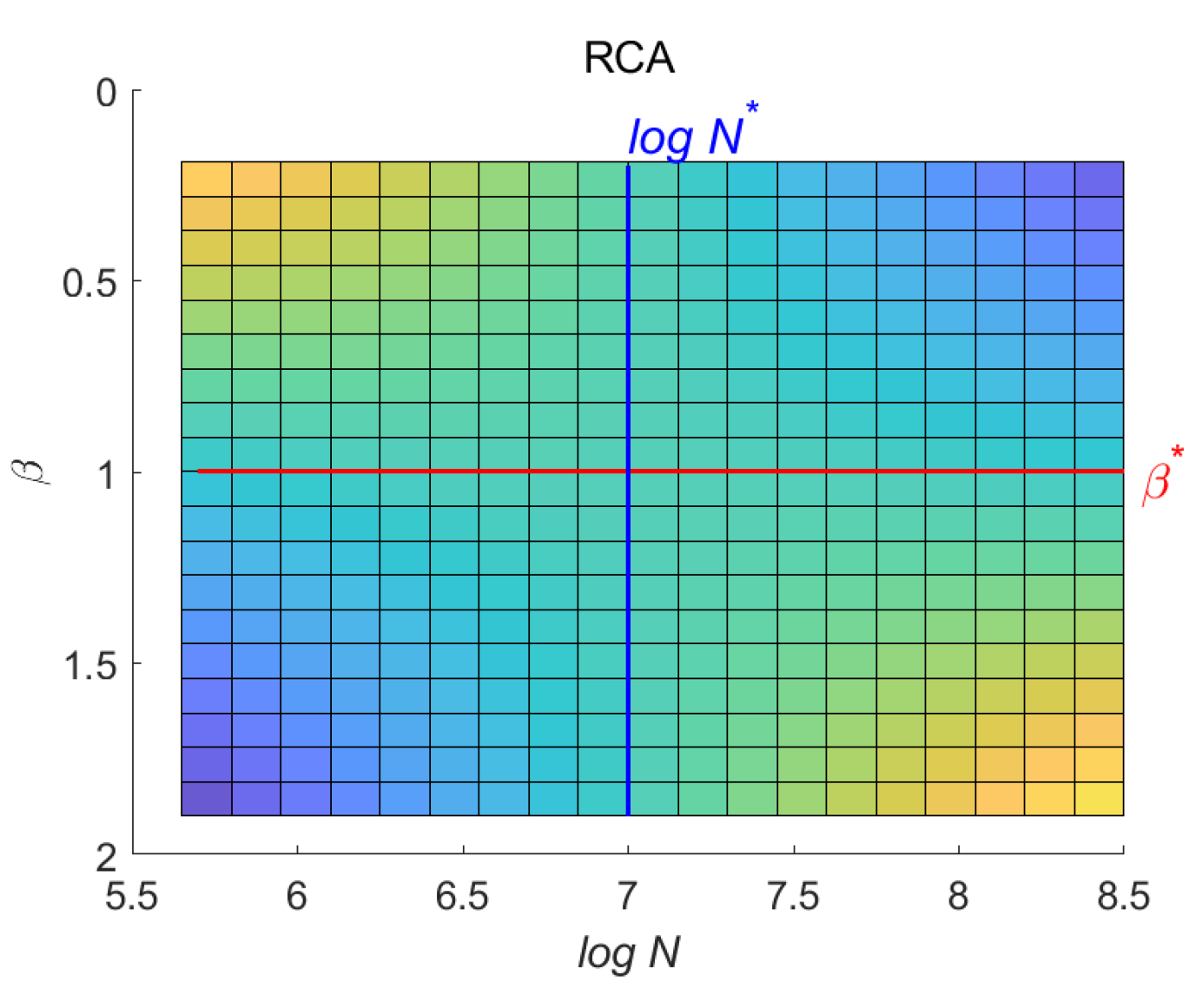
In this study, based on empirical analysis, the critical points are identified as saddle points with the Hessian matrix having one positive eigenvalue and one negative eigenvalue. Through a schematic diagram of this two-dimensional surface, the evolution of for different industrial employment with parameter changes is analyzed (see Figure 1). When , for industries with , increases with increasing , while for industries with , decreases with the growth of . This demonstrates that is an important critical point. The advantages of knowledge-spillover industries can only be realized when the urban population reaches a certain scale.
Figure 1.
Schematic diagram of a two-dimensional surface of , based on and .
4. Results
4.1. The Distribution and Evolution of Scale Characteristics
4.1.1. Evolution of Scale Characteristics
The hypothesis posits that the employment population in different industries and urban population adhere to a power-law relationship, described by . Here, varies across industries, reflecting different scaling effects. To test this hypothesis, a log-linearized model is employed for regression analysis. Additionally, a null model is introduced for comparison, which assumes that the employment population is determined solely by a constant term and is independent of urban population. Both the actual model and the null model are fitted using ordinary least squares (OLS), and an F-test is conducted to compare them. If the p-value of the F-test is less than the significance level (e.g., 0.05), it indicates that the actual model significantly outperforms the null model, thereby supporting the hypothesis that a power-law relationship exists between employment population and urban population, with distinct values for different industries.
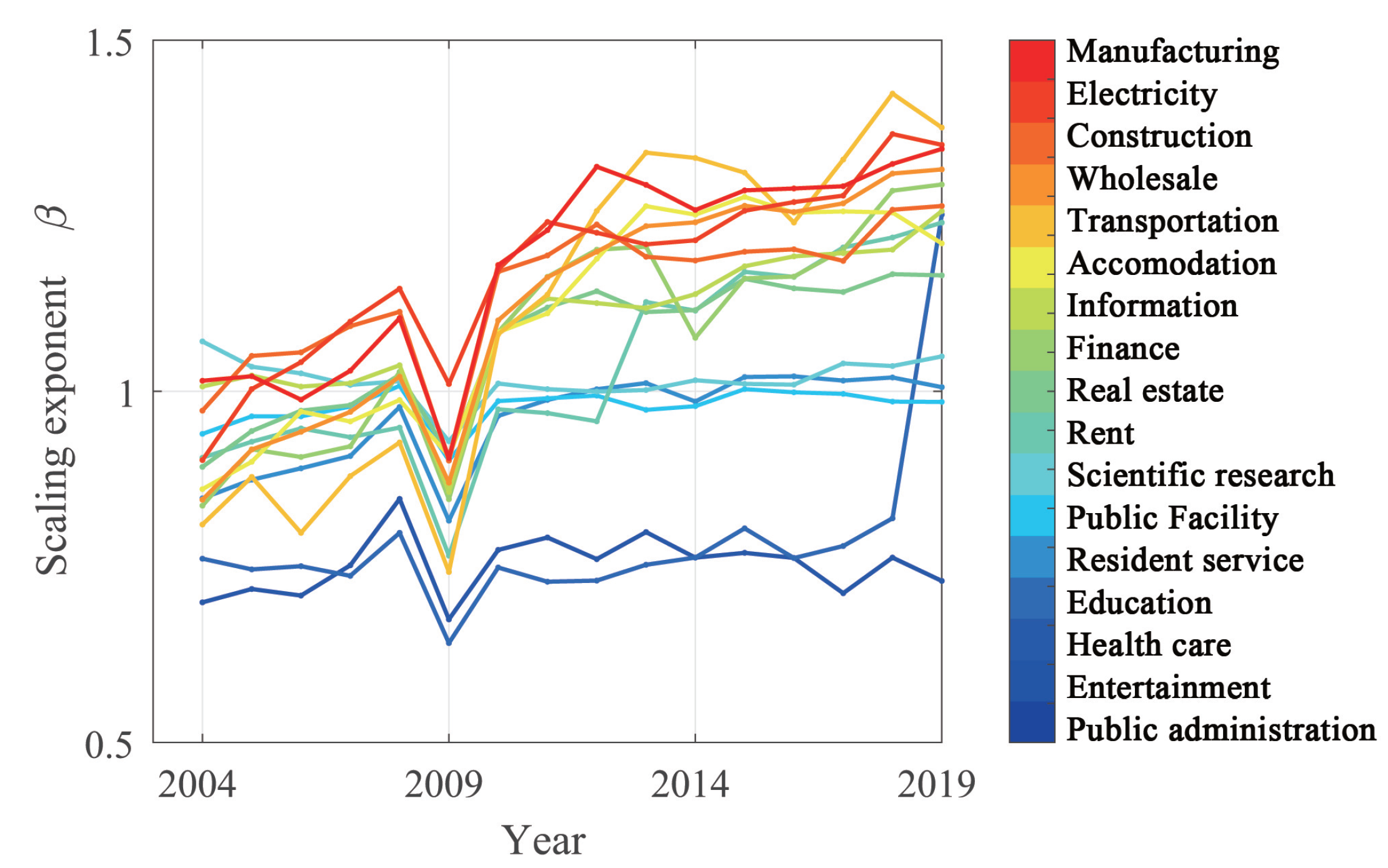
For the period 2004–2020, only the scaling relationships in the agriculture and mining industries are insignificant. This indicates that for most industries, there is a logarithmic linear relationship between employment and urban population , allowing the hypothesis to pass the test. For these two special industries, agriculture and mining, the scaling characteristics are not considered in subsequent research. Figure 2 shows that in China, around 50% of industries have . The distribution of is wider in 2019 than in 2004. Specifically, in 2004, fell within a narrower range of [0.7, 1.1], while in 2019, the range expanded to [0.7, 1.4]. The resident service, public facilities, and manufacturing industries are representative of those whose increased rapidly. There was no obvious decrease in during 2004–2019.
Different factor endowments and technology levels cause the same industry to have varying across different countries. Although scaling characteristics cannot be used to judge the advantages of an industry between China and the United States, indicates that the employment structure of that industry in large cities is more advantageous. The economies of scale in large cities show that industries with tend to be more important and often represent the driving force of the country’s economic development. Therefore, the development of “knowledge-spillover” cities should focus more on industries with .
The analysis compares the changes in scaling characteristics in industries and shows their longitudinal dynamics between 2004 and 2019, with manufacturing, finance, education, and public administration as four typical examples (see Figure A5 in the Appendix). The results show that the manufacturing industry has become more concentrated and the scaling effect stronger; education and public services have become more decentralized, with more equal resource allocation; and the financial industry has maintained a relatively stable relationship. The regression results for 2019, including and , indicate that the scaling relation captures the patterns of most cities.
Figure 2.
Time series of scaling exponents of industries in China.
4.1.2. Distribution of Scale Characteristics in Different Cities
It is generally believed that cities of different sizes have various advantageous industries. Based on the average population during 2004-2019 (without year 2009 because of its instability), it divided 280 cities into three groups: small, medium, and large cities (each comprising 33% of the total). Figure 3 shows the probability distribution of characteristic industries in the three groups. For all cities, more characteristic industries exhibit sublinear scaling with . For scaling exponent , the mean value () of large cities is higher than that of medium cities, and the of medium cities is higher than that of small cities. However, the standard deviation follows the opposite trend.
Figure 3.
The characteristic distribution of significant industries in cities of different sizes.
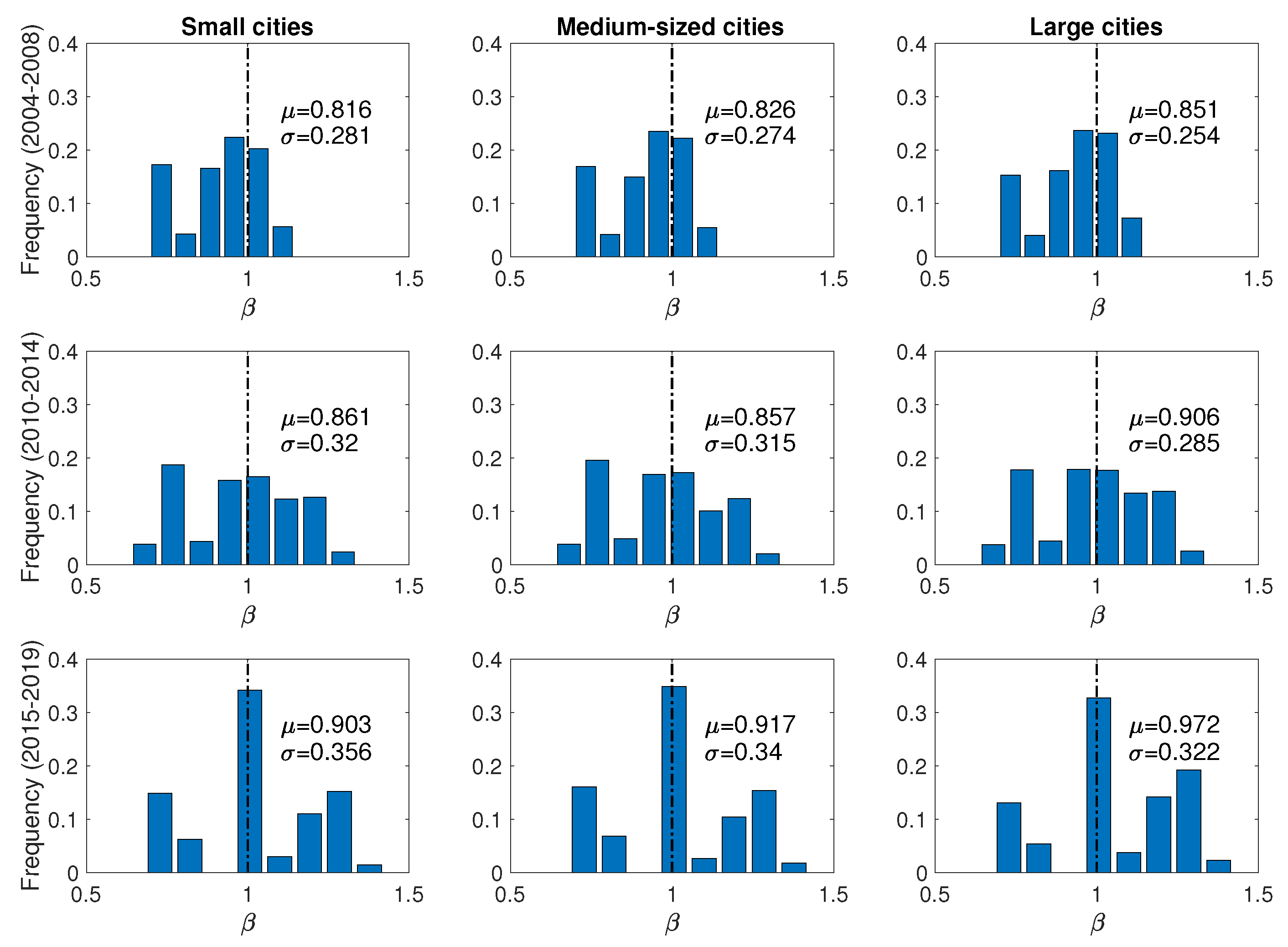
This analysis confirms that the advantageous industries in large cities are more likely to be knowledge spillover industries, while small cities have more significant infrastructure industries.
4.2. Labor Demand of “Knowledge-Spillover” Development
4.2.1. Evolution of Knowledge Spillover Industries
Existing literature indicates that population dependencies may underpin the urban economic structure and its evolution, as small cities heavily rely on infrastructure industries, while large cities rely on knowledge spillover ones [54,55,56]. This finding is also verified in Section 4.1.2. Furthermore, some scholars have analyzed data from the United States and propose that knowledge spillover industries become characteristic only when the urban population reaches a certain scale [7] (referred to as cognitive industries). Does this rule also apply to other economies? Here, it is shown that Chinese cities of different sizes have distinct characteristic industries. Although industrial scaling characteristics vary across countries, do they follow similar universal laws in “knowledge-spillover” development? As a populous country with rapid economic development, China’s urban evolution has attracted widespread attention. Chinese cities with characteristic knowledge spillover industries are defined as “knowledge-spillover” cities, and the path of “knowledge-spillover” development and their labor demand are studied using both theoretical models and empirical analysis.
Population size is not used to define “knowledge-spillover” cities here. However, subsequent analysis shows that the structural advantages of knowledge spillover industries often only appear in cities with sufficiently large populations, with the premise that the urban population of the country follows log-normal distribution characteristics, and the employment structure of infrastructure and knowledge spillover industries exhibit different growth (or scale) characteristics. Especially in China, compared with infrastructure industries, cities with advantageous knowledge spillover industries often require a population size of more than 10 million. This is a universal rule for the emergence of “knowledge-spillover” cities in China, as detailed below.
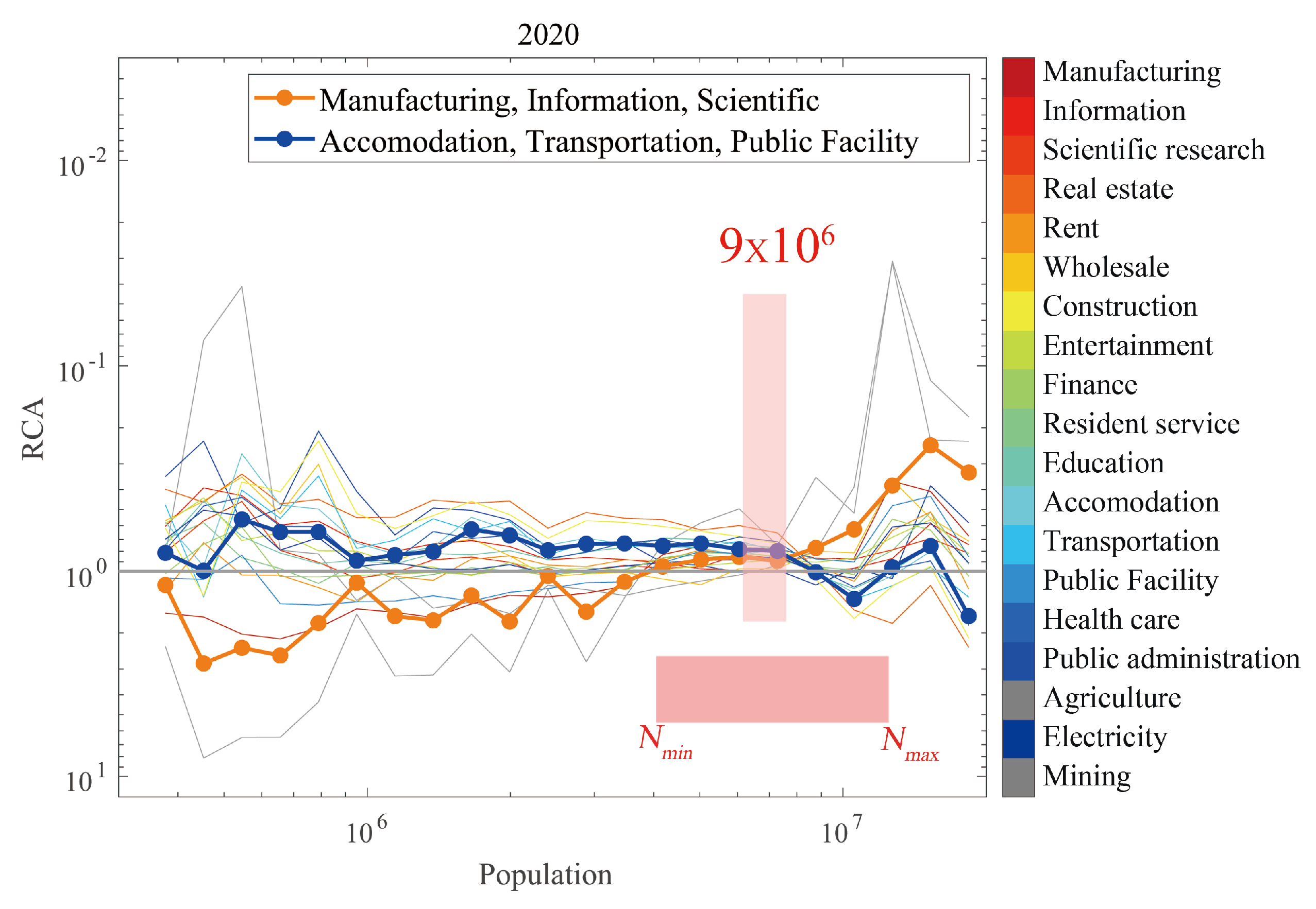
Figure 4 shows the average of 19 industries in cities with different population sizes in 2019. Here, the color of the line indicates the of the industry: blue for infrastructure industries, red for knowledge spillover industries, and gray for agriculture and mining industries. To make it clearer, the average evolution trends of several typical knowledge spillover and infrastructure industries are highlighted. It is emphasized that, based on the previous assumptions, only the effective region where there is a logarithmic linear relationship between urban population and employment is discussed, i.e., the regions between and .
Figure 4.
Average comparative advantage of Chinese cities of different sizes. Each line represents the of an industry in different cities, colored by the scaling characteristic of the industry, as . A value higher than indicates that the industry is significant in cities of this size. Source: Data from the “China City Statistical Yearbook” (2019).
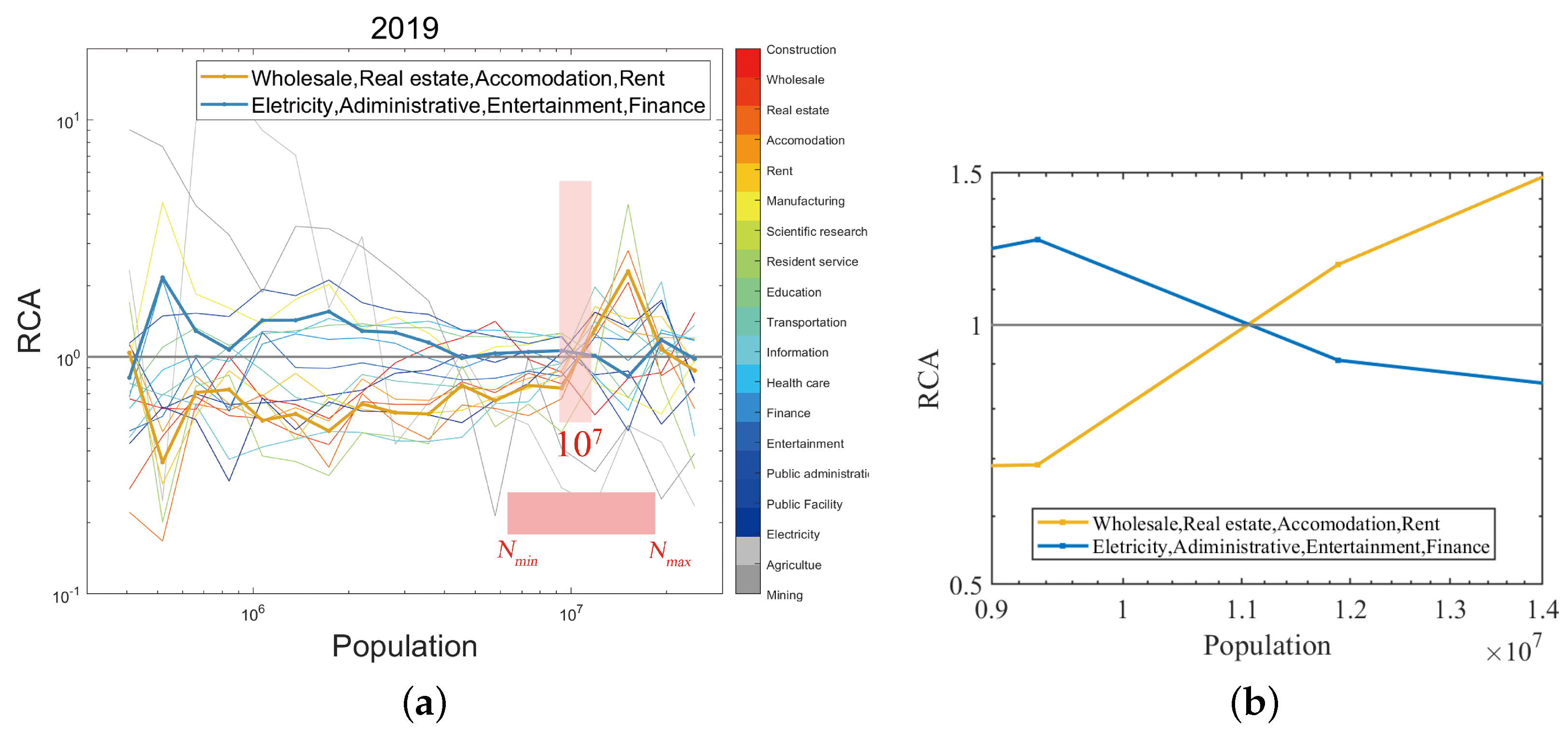
First, for small- and medium-scale cities in China, infrastructure industries (in blue) are usually more characteristic. With the expansion of urban scale, the of knowledge spillover industries (in red) increases, while the of infrastructure industries gradually decreases. When the population size reaches , the comparative advantage of cities shifts to knowledge spillover industries, whose values exceed those of infrastructure industries. This is similar to the urban development pattern in the United States, where the emergence of “knowledge-spillover” cities is based on a certain population size. “Knowledge-spillover” cities in the United States require less labor than Chinese cities, with a threshold of approximately [7].
After observing this phenomenon from the empirical data, it was analyzed with a theoretical model. Based on the analysis of Eq. 3, two critical points were identified, both of which are saddle points. Especially at the critical point where the urban population is around , the advantages of knowledge spillover industries become prominent, with . Meanwhile, the advantages of infrastructure industries disappear, with . The competitive strengths of these two types of industries are reversed at this point.
Here, has a maximum in one dimension and a minimum in the other dimension. The details are provided in the Appendix. According to the theoretical model, around these two critical points, the of knowledge spillover industries increases with urban population growth, while that of infrastructure industries decreases. Moreover, crossing the second critical point (the pink one) indicates that the significance of knowledge spillover industries exceeds that of infrastructure industries. This also implies that the emergence of “knowledge-spillover” cities is based on a certain urban population size, such as in China.
Therefore, both the empirical data and the theoretical model identify and verify the critical points, confirming the theoretical hypothesis and deduction process and revealing several statistical rules for comparative advantage in China’s urban evolution.
4.2.2. Comparison with the Optimal City Size Model
The critical point in China is around , while in the United States it is about . As analyzed in Section 4.2.3, in addition to the differences in absolute population (i.e., the various and in different countries), this difference mainly stems from the distribution characteristics of urban size in different countries, as indicated by . This idea is similar to the traditional optimal city size theory [57]. For a single city, finding the optimal size is a typical optimization problem that considers economic externalities or agglomeration benefits, as well as commuting and rental costs [58,59,60]. The optimal size of multiple cities in an urban system is usually measured by the rank-size rule [17,61,62], which is typically described by Pareto distribution, Zipf’s law, or some improved models [24,25,63]; or log-normal distributions [27,28].
Some scholars have calculated the optimal size of a single city in China and the United States. From the perspective of maximizing net income, Wang and Xia pointed out that the optimal city size in China is about [64]. Carlino studied the relationship between agglomeration economies and the increasing coefficient of scale returns from the perspective of increasing returns to scale, and pointed out that the optimal city size in the United States is about [65]. Using Carlino’s method as a reference, Jin pointed out that the optimal city size of Beijing, Shanghai, and Tianjin is around [66]. Of course, some studies that incorporate environmental pollution and energy efficiency suggest that the optimal city size obtained is significantly smaller than that suggested by previous research, and that the optimal urban size in China should not exceed [67,68]. Existing literature considers output as a whole, without discussing the dependence and impact of changes in output structure on city size.
Using one typical optimal size model of a single city5, it quantifies the optimal city size in China and the United States that maximizes benefits through the analysis of personal income and expenditure [57]. The results show that, based on the empirical data in 2019, the optimal city size in the United States is , while that in China is . The optimal size model differs from the method in this study, but both yield similar quantitative results (details in Appendix C.3).
In the optimal size model, represents the exponential rate of per capita GDP growth with urban population size. Both and describe the population-based scale effect and urban endogenous agglomeration benefits from different perspectives. China has a smaller and a larger (see Table A3 in Appendix). A smaller indicates that the population is more concentrated in a few large cities, while a larger indicates that per capita output or personal income is relatively higher in large-scale cities. These factors make China’s optimal city size much larger than that of the United States. Because the population is highly concentrated in a few large cities, fewer Chinese cities can cross the critical transition point compared to the United States.
The traditional optimal city size model describes the benefits of urban growth through economies of scale and analyzes the problems associated with congestion costs. Supplementing the discussion on changes in economic structure with urban scale growth would provide a valuable supplement and verification to the theory of optimal city size. The employment structure reflects a city’s production characteristics. The predominance of knowledge spillover industries often means higher per capita output under the same size. Thus, the evolution of the employment structure is related to changes in a city’s optimal scale, as illustrated by the consistency of results between the two models.
4.2.3. The Limitations of Urban Innovation in China
For cities located near the critical point, industries with show significant increases, while those with show decreases. Therefore, cities near are selected to analyze their evolution trends. As shown in Figure 5, some of these cities are on the verge of surpassing and have the potential to transform into “knowledge-spillover” cities, including Guangzhou, Baoding, Shijiazhuang, Suzhou, Linyi, Shenzhen, Chengdu, and Wuhan. In addition, three cities—Beijing, Shanghai, and Chongqing—have already surpassed the critical point in terms of population size, despite not being located near it. Here, subinnovative cities refer to the emergence stage of the innovation cycle. Compared with the stage of subinnovative cities that have leading technologies and highly skilled jobs, cities in the “knowledge-spillover” stage have more mature technologies and a higher density of skilled jobs [11]. Moreover, of cities in China still need to further improve their technical levels and work proficiency to achieve “knowledge-spillover” development.
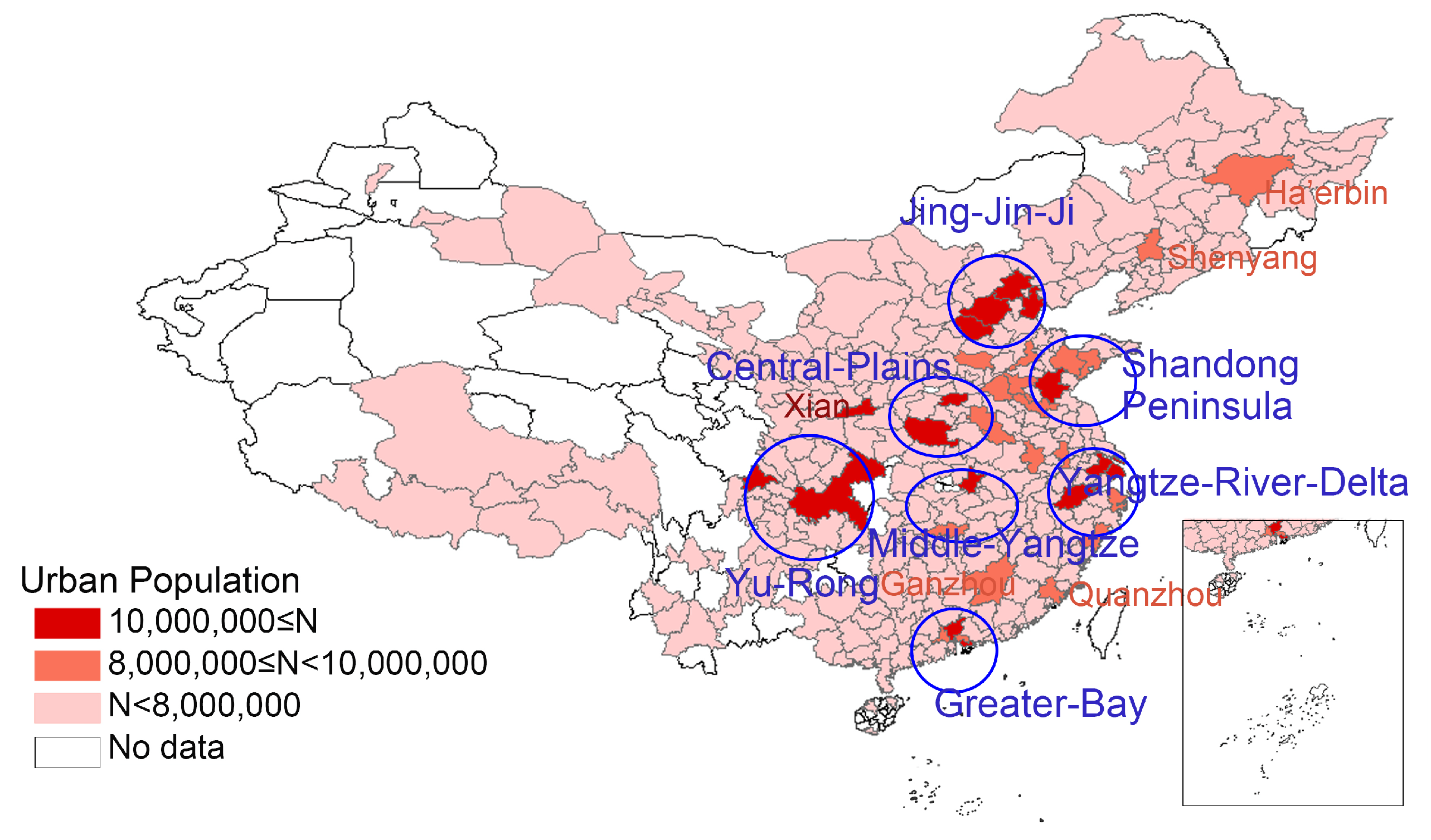
Figure 6 analyzes the geographical distribution of cities near the critical point. Dark red indicates cities that have crossed , while light red indicates cities with a population gap of less than 20% from . In terms of spatial distribution, all “knowledge-spillover” cities are concentrated east of the Hu Huanyong Line, which marks regions with relatively high population density in China. Moreover, most dark red and light red cities are located in China’s major urban agglomerations, including the Central Plains, Jing-Jin-Ji, Shandong Peninsula, Yangtze River Delta, Yu-Rong, Middle Yangtze, and Greater Bay areas (marked here).
Figure 5.
Cities near the critical point. represents rough average critical points. Different colors represent different cities. Cities near these points are selected to observe the change in the population of these cities over time. Source: Data from the “China City Statistical Yearbook” (2004-2019).
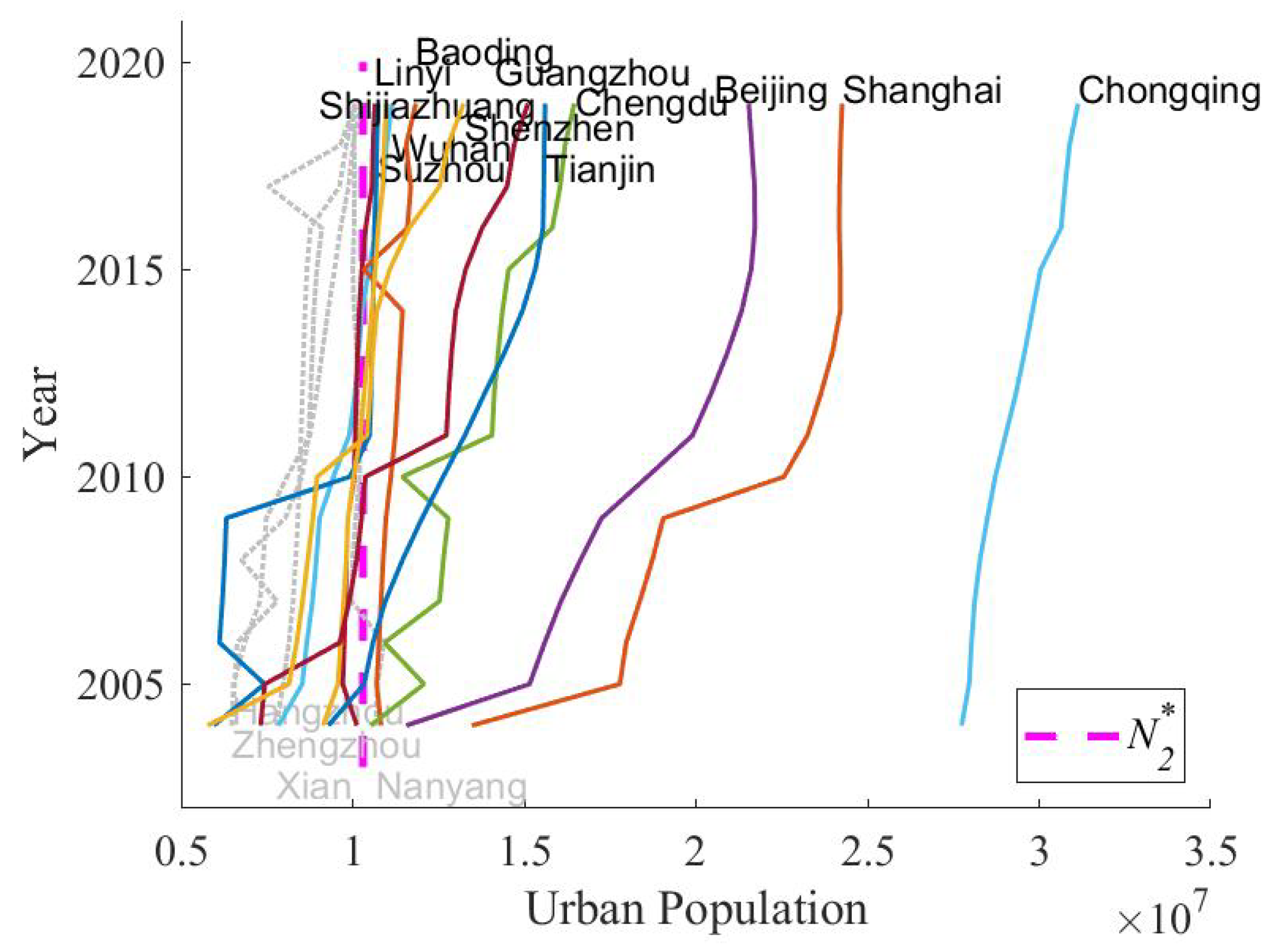
Figure 6.
The distribution of cities with populations near the critical point in 2019. The darkest red color represents the districts larger than the critical point, the lighter red represents the districts below the critical point , the lightest color represents the districts below of the critical population size, and the white areas have no statistical data. Source: Data from the “China City Statistical Yearbook” (2019).
This indicates that the proportion of Chinese cities crossing or near the critical point is relatively low. According to statistics from the United States Census Bureau in 2019 [69], among the 384 metropolitan statistical areas, 49 metropolitan areas have populations exceeding the critical population size of 1.2 million [7], accounting for . Therefore, in China, there are not enough cities likely to complete the transformation from subinnovative to “knowledge-spillover” cities. Moreover, most of these cities are located near existing “knowledge-spillover” cities. When these cities complete the transformation, they can form urban agglomerations of a certain scale, which will facilitate further regional expansion.
China is a populous country. In terms of absolute population size, most Chinese cities have larger populations than their U.S. counterparts. Even in 2019, 256 prefecture-level and above cities had populations exceeding the critical point of the United States (i.e., 1.2 million). However, due to differences in urban population distribution and industrial employment scaling characteristics, the demand for population resources in “knowledge-spillover” cities varies significantly between the two countries. This is related to factors such as production technology and other economic conditions. Only 16 cities in China meet the population demand for “knowledge-spillover” development, and the innovation rate of population demand is far lower than that of the United States.
4.2.4. Influence of Population Distribution Characteristics
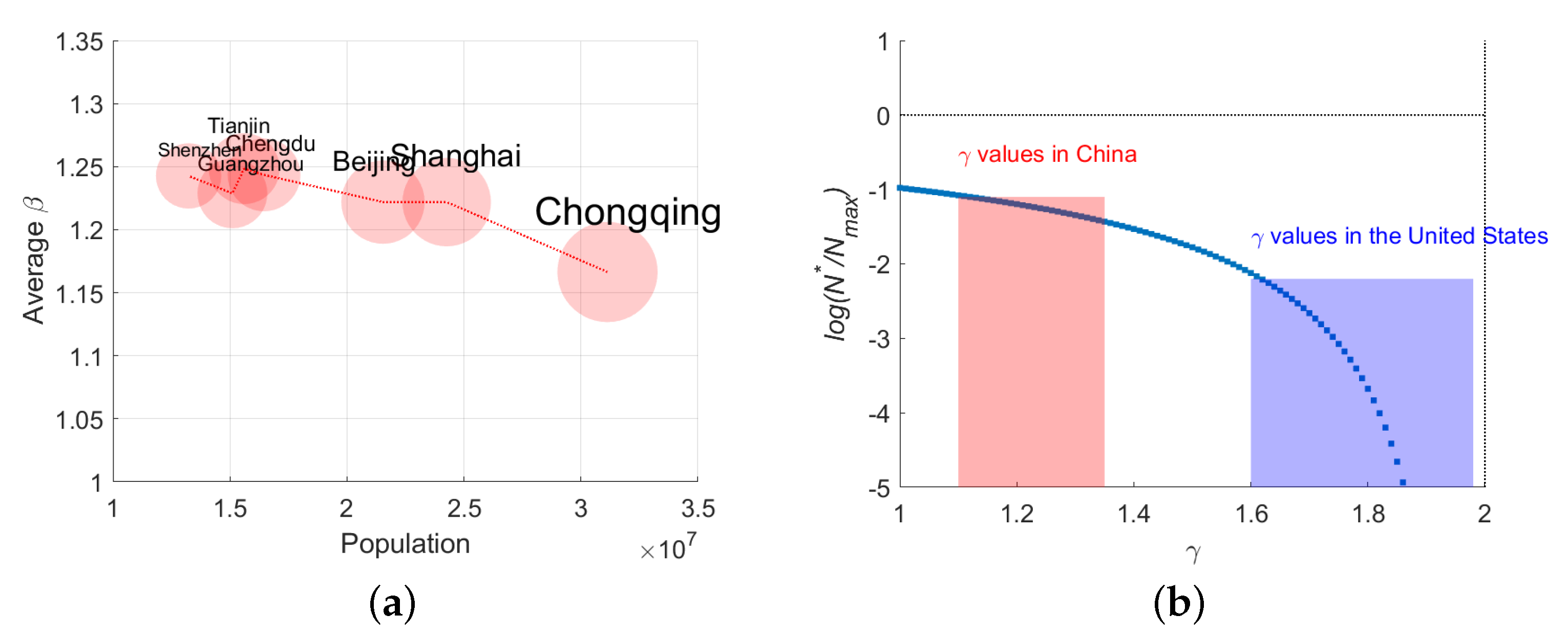
In addition, to compare economies of different population sizes, it theoretically analyzes the changes in according to different values of . represents the distribution characteristic of the urban population in a country and has a significant impact on the proportion of “knowledge-spillover” cities. It is generally believed that the of the United States is less than 2 [7], while the of China is located in . Consequently, is closer to 0 in China compared with the United States. Therefore, the population demand of China’s “knowledge-spillover” cities is closer to that of the largest cities, indicating a limited number of such cities in China (Figure 7(b)).
Besides, the trend of urban population growth in China is not encouraging [70]. China’s population has already experienced three consecutive years of negative growth [71]. According to the latest data, the total population reached a peak in 2022 and has been declining since then. In 2024, the total population decreased by 139 million compared to the previous year, with a natural growth rate of -0.99‰.
Furthermore, according to the latest projections, China’s working-age population is expected to continue declining at an accelerated pace, with a projected decrease of 200 million people by 2050 [72]. The slow or even negative growth of China’s population will lead to significant changes in population structure, which will greatly impact urban innovation capabilities [73]. At the same time, China’s large cities will face challenges related to industrial agglomeration and innovation agglomeration [74].
Figure 7.
(a) average of largest cities in China. (b) changes of according to different
5. Conclusion & Suggestions
Exploring the conditions for the emergence of cities dominated by “knowledge-spillover” industries is of great significance. These cities leverage superlinear growth factors to achieve advanced development and utilize resources more efficiently. Focusing on China, this study identifies a development path in urban evolution and the labor demand characteristics of “knowledge-spillover” cities through the analysis of industrial employment and comparative advantage. It uncovers a critical population size.
1. The Comparative Advantage of “Knowledge-Spillover” Industries Requires a Critical Urban Population Size
The relationship between industry employment and urban population reveals distinct growth patterns for different industries. Superlinear growth industries, such as “knowledge-spillover” industries, accelerate their growth in larger cities, which can be interpreted as a more efficient aggregation of resources. This phenomenon is observed in the statistical patterns of urban population and employment numbers in prefecture-level cities in China. The analysis from a modeling perspective further elucidates the underlying mechanisms.
The log-normal distribution of urban population indicates that only a small number of large-scale cities exist. Industries have different scaling effects: sublinear growth industries typically dominate in smaller cities, while superlinear growth industries thrive in larger cities. The comparative advantage of superlinear growth industries over sublinear growth industries emerges when the urban population reaches a certain scale. This critical population size varies across economies, depending on urban population distribution characteristics and the scaling properties of different industries.
2. The Critical Population Size of 10 Million for China
The specific superlinear growth industries vary across countries due to differences in economic endowments, production technologies, and other factors. For instance, in the United States, administrative and financial services exhibit superlinear growth characteristics, while in China, manufacturing and retail trade are more prominent. The underlying principle is the same: each country has industries that can grow at an accelerated rate, aggregating resources more efficiently and driving economic development more effectively. These industries can only thrive as “knowledge-spillover” and dominant sectors in cities that reach a certain population size.
The labor demand for “knowledge-spillover” cities varies between economies. In the United States, it is approximately , while in China, it is . This difference is influenced by the overall population size and the characteristics of urban population distribution. China’s urban population distribution has a larger negative power index compared to the United States, indicating a relative insufficiency in the number of large cities. Despite China being a populous country, only 5.7% of its cities have become “knowledge-spillover” cities, compared to 12.8% in the United States.
3. Future Prospects for China
The critical population size of 10 million in China represents a significant threshold. However, this threshold is particularly high given the current trends in China’s demographic and urban development. China’s population growth has been slowing down, and the further expansion of megacities could lead to several challenges. The expansion of large cities may result in urban problems such as traffic congestion, housing shortages, and environmental pressures, commonly referred to as “metropolitan malaise”. The concentration of population in a few megacities could exacerbate the imbalance in urban population distribution, potentially raising the threshold even higher.
To address these challenges and leverage the advantages of superlinear growth industries, China needs to adopt a balanced urban development strategy. This strategy should focus on promoting the growth of medium-sized cities and improving the connectivity and integration of urban agglomerations. By doing so, China can create a more balanced urban population distribution, reduce the pressure on megacities, and provide more opportunities for the emergence of knowledge-spillover cities. Additionally, policies should be designed to encourage the development of superlinear growth industries in a wider range of cities, ensuring that the benefits of these industries are more evenly distributed across the country.
Appendices
Author Contributions
Xiaohui Gao (first author): data curation, formal analysis, writing - original draft. Qinghua Chen: supervision, methodology, validation. Ya Zhou (corresponding author 1): Data curation , supervision, writing - review & editing. Siyu Huang (coauthor): conceptualization, formal analysis, methodology, writing - original draft. Yi Shi (coauthor): conceptualization, supervision, validation. Xiaomeng Li (corresponding author 2): formal analysis, supervision, writing - original draft, writing - review & editing. All authors have read and agreed to the published version of the manuscript.
Funding
This work was supported by National Social Science Foundation (22BRK021), and the Interdisciplinary Construction Project of Beijing Normal University.
Acknowledgments
We appreciate the comments and helpful suggestions from Professors Dahui Wang, Zengru Di and Handong Li.
Conflicts of Interest
The funders had no role in the design of the study; in the collection, analyses, or interpretation of data; in the writing of the manuscript; or in the decision to publish the results.
Appendix A. Data Source and Statistical Analysis
Appendix A.1. Cities & Industries
Appendix A.1.1. The Cities in China
In China, one of the administrative divisions is the city, which is typically categorized into three types based on different administrative statuses: 1. municipalities directly under the central government, which are part of provincial-level administrative regions; 2. prefecture-level cities, which belong to prefecture-level administrative regions; and 3. county-level cities, which are part of county-level administrative regions. By the end of 2020, China had a total of 685 cities, including 4 municipalities directly under the central government, 293 prefecture-level cities, and 388 county-level cities. Since the definition of urban agglomeration in China is not unified, urban planning and development are still implemented by the municipal governments of municipalities directly under the central government, prefecture-level cities, and county-level cities. This study primarily refers to the administrative divisions of cities by the Chinese government, as they more closely align with the realities in China. Prefecture-level cities are commonly used as a scale unit for analyzing the urban economy in China. Additionally, the data in this study adopt the statistical caliber of “the whole city”, which includes urban areas, counties, and cities, covering the entire range of prefecture-level cities, rather than including only urban areas.
Appendix A.1.2. Municipalities and Prefecture-Level Cities
Since 2019, China has had 4 municipalities directly under the central government and 293 prefecture-level cities, making a total of 297 cities. For this study, we selected 280 of them. Specifically, 16 cities were excluded due to the lack of Gross Regional Product (GRP) data for several years, which also affected the availability of resident population data (these cities are Sansha, Zhangzhou, Bijie, Zunyi, Tongren, Lasa, Rikaze, Changdu, Linzhi, Shannan, Naqu, Longnan, Haidong, Zhongwei, Turpan, and Hami). Additionally, 2 cities were excluded due to the absence of employment population data for certain industries (Ziyang and Hengshui). In total, these 18 cities were excluded from the analysis. Furthermore, Laiwu was merged into Jinan in January 2019, but it was retained in the analysis to maintain consistency. Considering the completeness of data, 280 municipalities and prefecture-level cities were ultimately used in this study.
The resident population can fully reflect the mobility characteristics of the current Chinese population and accurately depict the urbanization level based on the resident population standard. According to the spirit of the 28th Executive Meeting of the State Council, the National Bureau of Statistics issued the Notice on Improving and Standardizing Regional GDP Accounting on January 6, 2004. This notice required provinces, autonomous regions, and municipalities to uniformly calculate per capita GDP using the resident population (i.e., the registered population minus the outflow population of more than half a year, plus the inflow population) in the future.
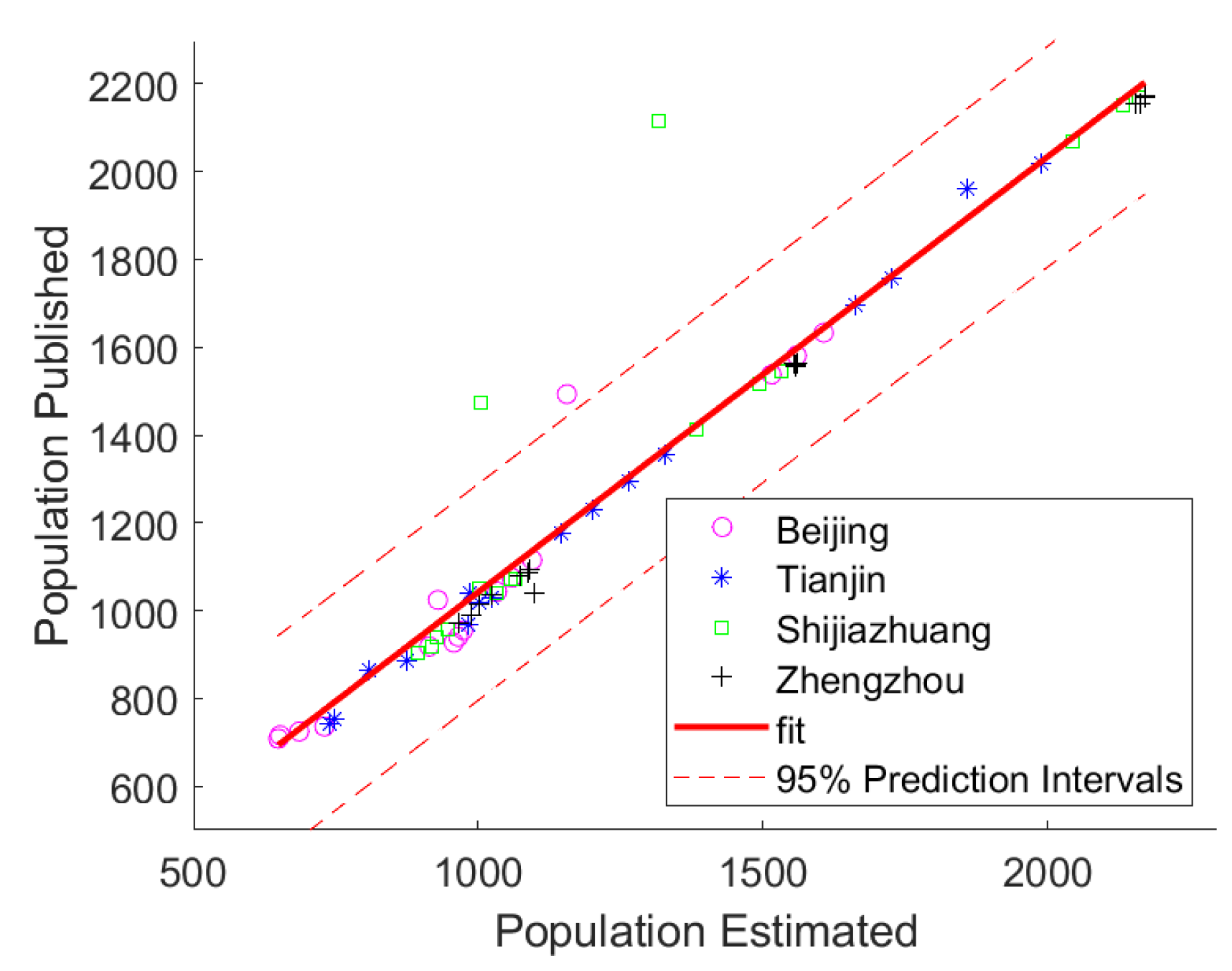
To estimate the urban population of each city, we used the formula , as many cities have not publicly released local resident population data. We selected four representative cities and compared the published urban population data with the estimated results. The results passed the t-test (with sig.=0.0107), indicating that there is no significant difference between the two groups of data. In the linear fitting analysis, the adjusted value was 0.9237 (see Figure A1).
Figure A1.
Reliability of the estimated data (in 10 thousand). Source: Estimated data from the "China City Statistical Yearbook" (2019) and published data from the statistical bureaus of cities.
Figure A1.
Reliability of the estimated data (in 10 thousand). Source: Estimated data from the "China City Statistical Yearbook" (2019) and published data from the statistical bureaus of cities.
Appendix A.1.3. 19 Industries
According to the latest classification (GB/T 4754-2017), China’s industries are divided into 20 categories. The industry related to “international organizations” is not included in economic statistics. Thus, it focus on the remaining 19 industries.
Details of the data are shown in Table 1, which shows that China’s urban population satisfies the log-normal distribution in 2019 (Figure A2), and this characteristic persists from 2004 to 2019.
Figure A2.
Distribution characteristics of urban population in China. (a) Lognormal distribution of urban population in China. (b) Approximate scaling exponent of Chinese cities in 2019. Source: Data from the “China City Statistical Yearbook” (2019).
Figure A2.
Distribution characteristics of urban population in China. (a) Lognormal distribution of urban population in China. (b) Approximate scaling exponent of Chinese cities in 2019. Source: Data from the “China City Statistical Yearbook” (2019).
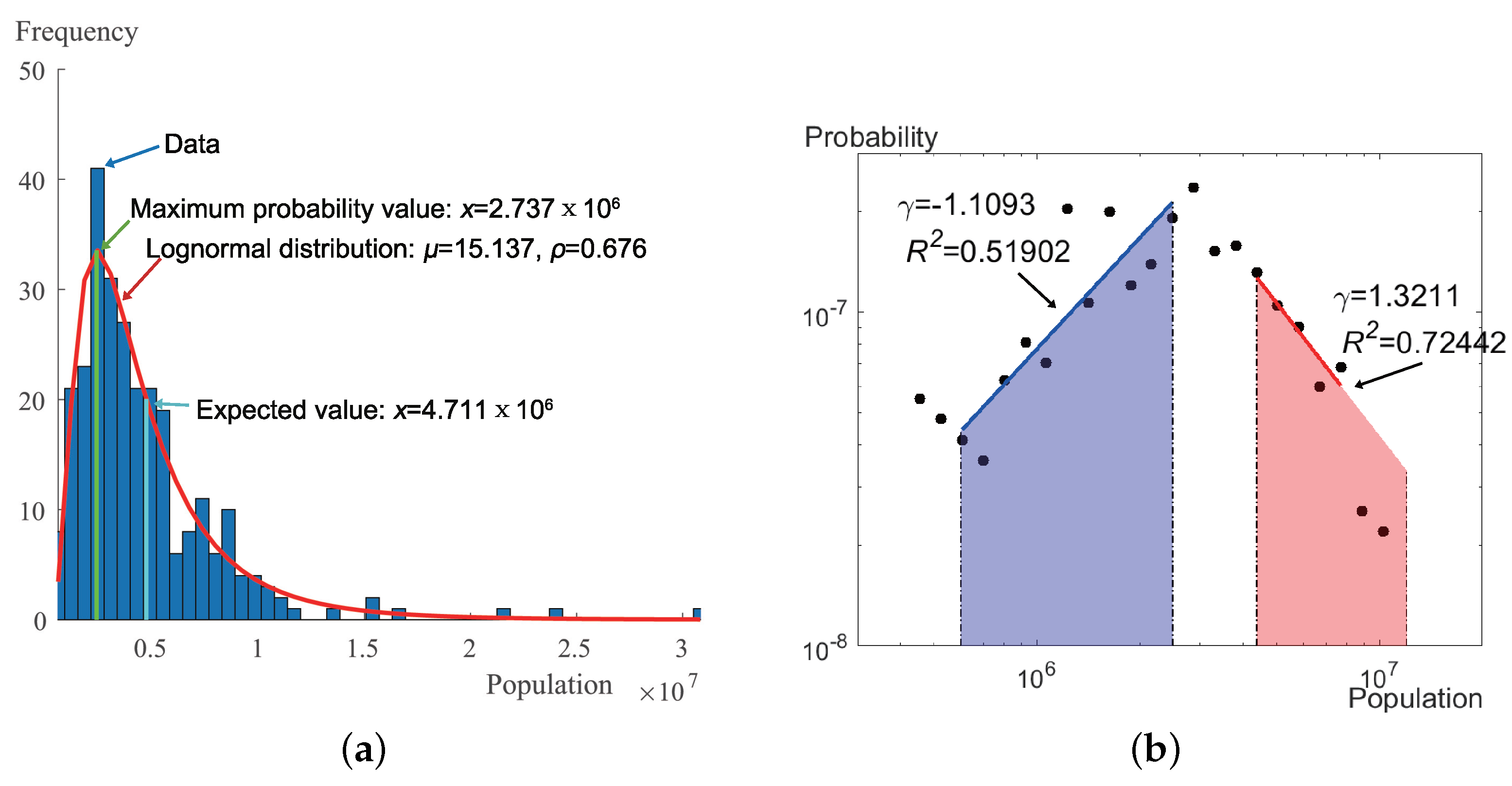
Figure A3.
Average comparative advantage of Chinese cities of different sizes (2020). Each line represents the of an industry in different cities, colored by the scaling characteristic of the industry, as . A value higher than indicates that the industry is significant in cities of this size. Source: Data from the 7th National Population Census (2020), National Bureau of Statistics, China.
Appendix A.2. Data Source
Appendix A.2.1. Explanation on the Time Interval of Data
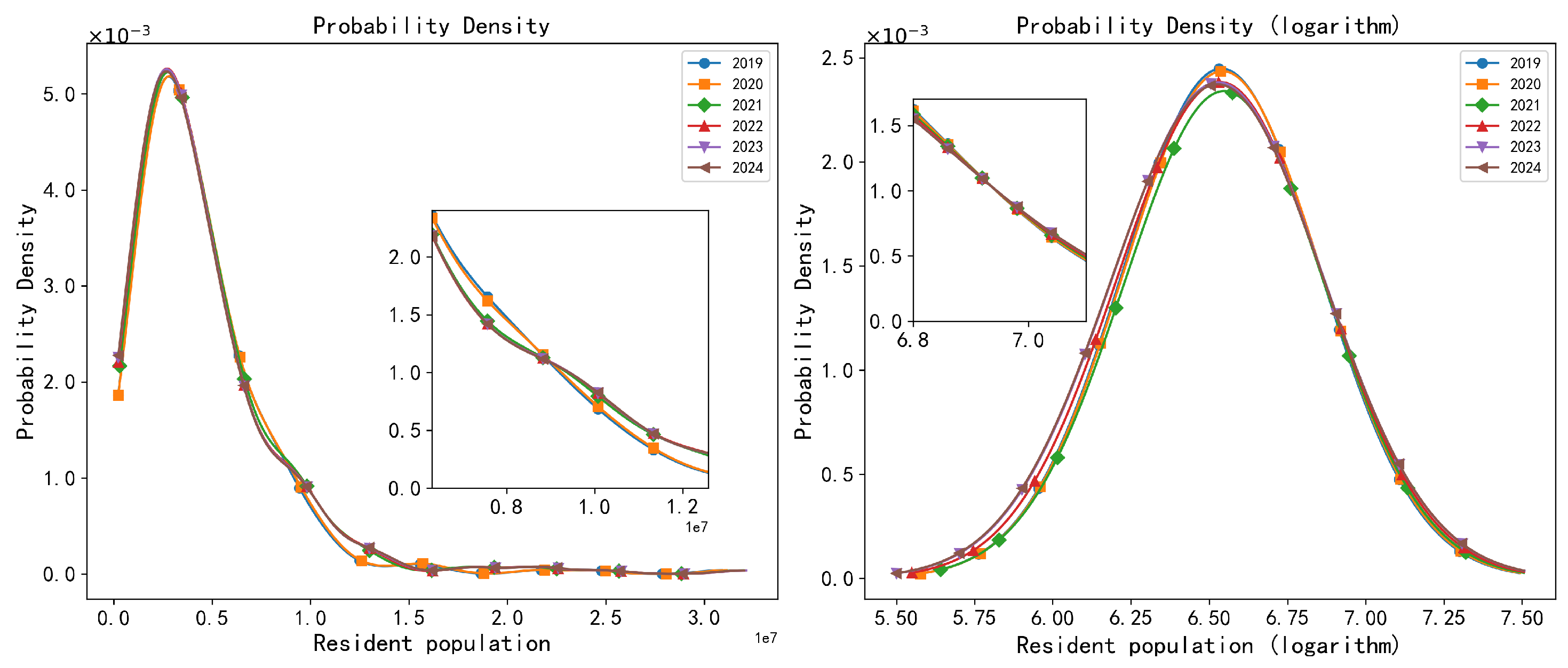
Since the “China City Statistical Yearbook” ceased reporting industry-specific employment data for prefecture-level cities starting from 2020, our dataset is confined to the period up to 2019. Additionally, Figure A4 shows the resident population of prefecture-level cities from the “China City Statistical Yearbook” for the years 2019–2024. After conducting the Shapiro-Wilk test, it was determined that these distributions follow a log-normal distribution, and the probability density functions of the log-normal distribution were fitted. Specifically, a comparative analysis was conducted of the distribution characteristics near . It can be observed that the temporary increase in the number of cities with populations less than during 2020–2021 gradually disappeared in 2022–2024, returning to the characteristics observed in 2019. Therefore, it is appropriate that the analysis in the main text concludes with the year 2019.
Figure A4.
The probability density of the resident population (2019-2024). Source: Data from the “China City Statistical Yearbook” (2019-2024).
Figure A4.
The probability density of the resident population (2019-2024). Source: Data from the “China City Statistical Yearbook” (2019-2024).
The population census in China is conducted every ten years. In 2020, data from the seventh population census were released, which includes employment population statistics by industry for prefecture-level cities. This data is used to conduct an analysis for the year 2020. Due to the differences in datasets, to ensure the validity and scientific nature of the study, this content has been included only in the appendix as supplementary information (see Appendix C.1).
Appendix A.2.2. Data Interpolation Method
If data for a certain industry are missing in only a few years, the approach can be divided into two cases: (a) For missing data in non-endpoint years (for example, within the time range of 2004–2019, the endpoint years are 2004 and 2019, while 2005–2018 are non-endpoint years), the linear interpolation method is used. This method requires that the data for adjacent years with missing values are not null. (b) For missing data in endpoint years, linear regression is used. Here, the evolution trend of the data can be quantified, making linear regression suitable for estimating endpoint values.
Appendix A.2.3. Logarithmic Linear Correlation of Population and Employment in Specific Industries.
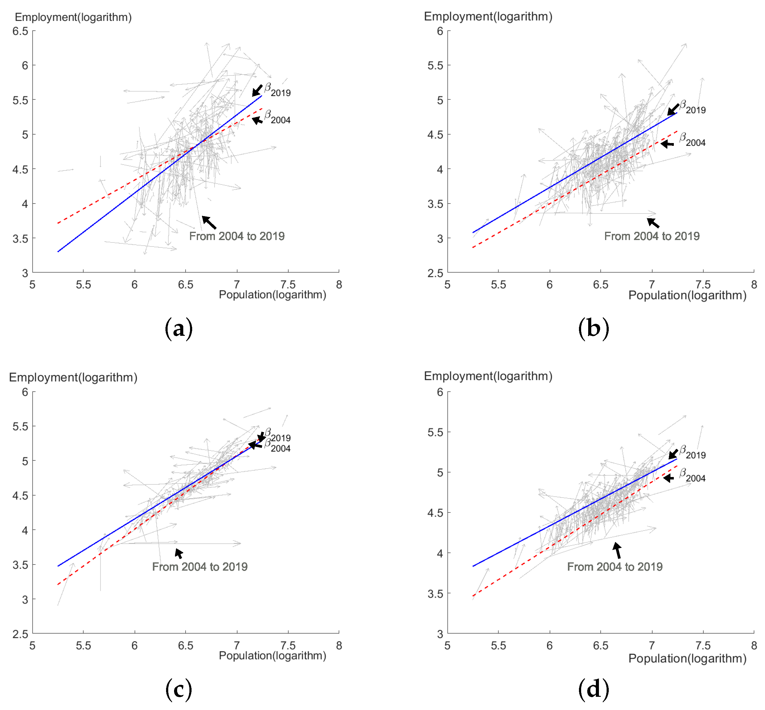
In Figure A5, each grey dot represents a city, with the x-coordinate indicating urban population and the y-coordinate indicating employment. The grey arrow indicates the directional change in each city’s position from 2004 to 2019. The red line represents the fitted relationship in 2004, while the blue line represents the fitted relationship in 2019. If the blue line is steeper than the red line, it indicates an increase in , as seen in the manufacturing industry. Conversely, a flatter blue line indicates a decline in scaling characteristics, as observed in education and public administration. For the financial industry, remains relatively stable, while overall employment across cities has increased. This suggests that the manufacturing industry has become more concentrated, with a stronger scaling effect; education and public services have become more decentralized, reflecting a more equal allocation of resources; and the financial industry has maintained a relatively stable relationship. The regression results for 2019, including and (see Table A1), indicate that the scaling relationship captures the patterns of most cities.
Figure A5.
Relationship of population and employment in specific industries. (a) Manufacturing. (b) Finance. (c) Education. (d) Public Administration.
Figure A5.
Relationship of population and employment in specific industries. (a) Manufacturing. (b) Finance. (c) Education. (d) Public Administration.
Appendix A.2.4. The Different β i for China and the United States
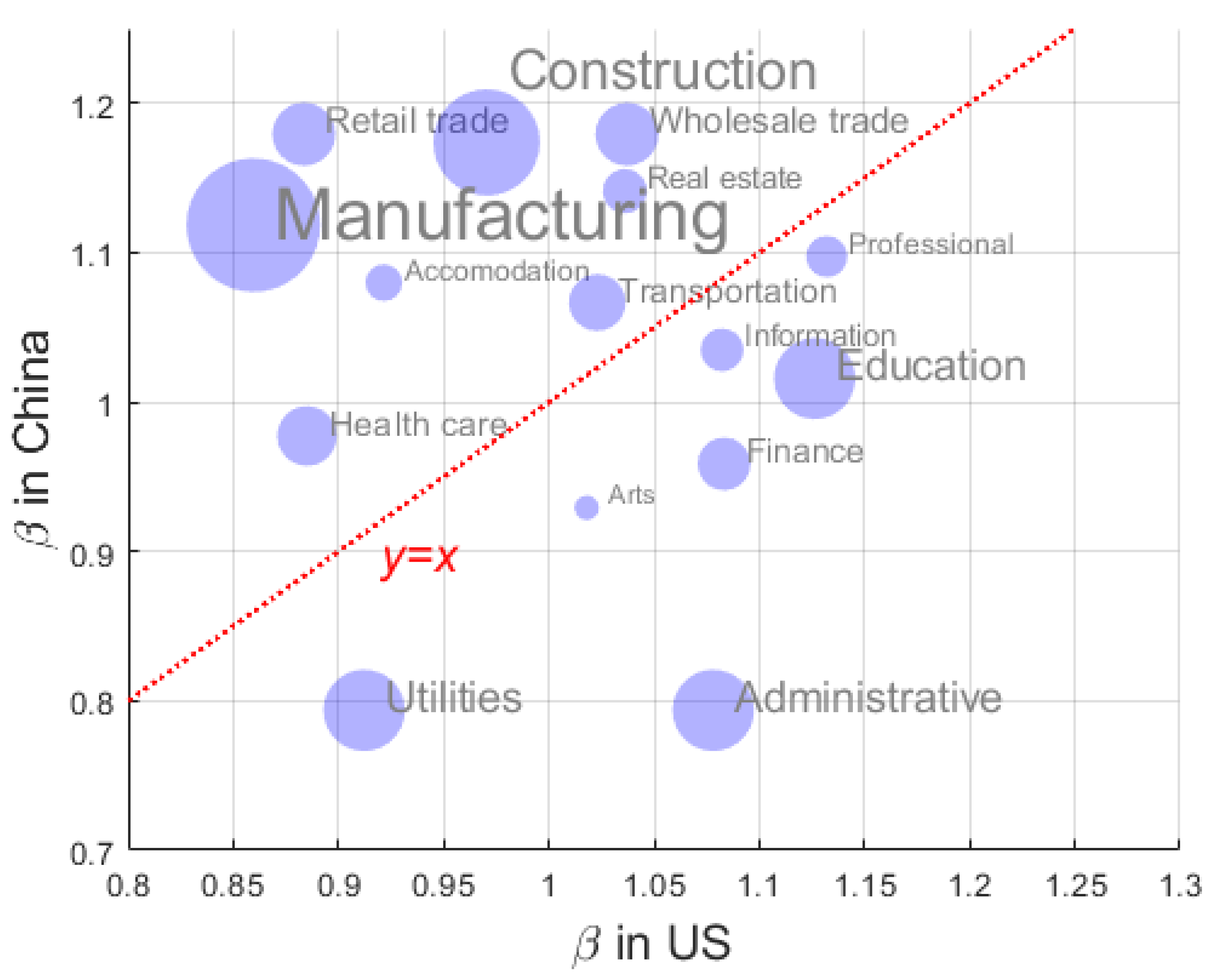
The same industry can exhibit different properties in different countries. Figure A6 shows that China and the United States have distinct characteristics in scaling exponents. Here, each dot represents an industry. The size of the dot and its label font indicate the employment scale of the industry in China. The x-coordinate shows the average of the industry in the United States during 2004–2019 [7], and the y-coordinate shows the corresponding value in China during the same period. The red line represents the line. Industries above the red line have relatively larger scaling exponents in China, while those below the red line have smaller scaling exponents in China. This indicates that the industrial scaling characteristics between China and the United States are quite different.
In the lower-right region of Figure A6, administrative services, finance, and the arts are superlinear industries in the United States but sublinear industries in China. In the upper-left region, manufacturing, retail trade, and health care are superlinear industries in China but sublinear industries in the United States.
Figure A6.
Correlation between scaling exponents in China and the United States.
Appendix B. The Theoretical Model and Derivation Process
Appendix B.1. The Scaling Laws for Cities
Zipf distributions of city sizes have been widely recognized [75,76]. In the past decade, it has been determined that most urban indicators follow the ubiquitous scaling law [9]:
Here, represents the population size of a city at time t; is a time-dependent normalization constant. can be different types of urban indicators. The existing literature indicates that represents the sublinear regime, which is associated with economies of scale in the surface area. In contrast, represents the superlinear regime, which is associated with outcomes from social interactions, such as R & D employment, inventors, supercreatives, and income.
Some scholars have used scaling laws to analyze the effects of urban spatial concentration on economic development. They observed that scaling exponents can be explained by the level of complexity of an activity, which may explain why complex economic activities are more concentrated in large cities [4,77]. These activities include research papers, patents, occupations, and industries. Later studies used employment data from different industries as urban indicators to analyze the evolution of infrastructure and knowledge spillover industries, based on data from the United States [7,54].
Table A1.
Scaling exponents in different industries
| Industry | ||||
|---|---|---|---|---|
| Agriculture, forestry, animal husbandry and fishery | 0.24 | 0.05 | 0.01 | 0.05 |
| Mining | 0.09 | 0.68 | 0.00 | 0.85 |
| Manufacturing | 1.32 ** | 0.00 | 0.52 | 0.00 |
| Production and supply of electricity,heating, gas,and water | 0.73 ** | 0.00 | 0.36 | 0.00 |
| Construction industry | 1.35 ** | 0.00 | 0.53 | 0.00 |
| Wholesale and retail | 1.35 ** | 0.00 | 0.61 | 0.00 |
| Transportation, warehousing, and postal services | 1.16 ** | 0.00 | 0.56 | 0.00 |
| Accommodation and catering industry | 1.29 ** | 0.00 | 0.44 | 0.00 |
| Information transmission, computing and services, and software | 1.24 ** | 0.00 | 0.54 | 0.00 |
| Finance | 1.01 ** | 0.00 | 0.57 | 0.00 |
| Real estate industry | 1.26 ** | 0.00 | 0.53 | 0.00 |
| Rent | 1.21 ** | 0.00 | 0.49 | 0.00 |
| Scientific research, technical services and geological survey | 1.26 ** | 0.00 | 0.51 | 0.00 |
| Public facilities management industry | 1.25 ** | 0.00 | 0.51 | 0.00 |
| Residential services, repair and other services | 1.38 ** | 0.00 | 0.41 | 0.00 |
| Educational Services | 1.05 ** | 0.00 | 0.93 | 0.00 |
| Health care and social work | 0.98 ** | 0.00 | 0.88 | 0.00 |
| Culture, sports and entertainment | 1.03 ** | 0.00 | 0.53 | 0.00 |
| Public administration, social security and social organization | 0.76 ** | 0.00 | 0.80 | 0.00 |
| ** indicates the significant industries every year at the 95% confidence level. | ||||
| : p-value for the regression coefficient. | ||||
| : p-value from the F-test, indicating the overall significance of the regression model. | ||||
| Source: Data from the “China City Statistical Yearbook” (2004-2019). | ||||
Appendix B.2. The Comparative Advantage Function
is the employment of industry i in city c.
An industry is called characteristic or significant if . The employment is proportional to the population of city as . With
it could get,
Appendix B.3. Changes in Comparative Advantage
- Changes with N.when , ; , ; and , .
-
Changes with ..In 2019,, , , when , . When , ; , ; , ., , , when , . When , ; , ; , .
Appendix C. Other Results
Appendix C.1. The Derivation Process on 2020 Data
Based on the data from the seventh population census was released, it gives the derivation process on 2020 as,
In 2020,
, , , when , . When , ; , ; , .
, , , when , . When , ; , ; , .
Figure A7.
Distribution characteristics of urban population in China. (a) Lognormal distribution of urban population in China. (b) Approximate scaling exponent of Chinese cities in 2020. Source: Data from the 7th National Population Census (2020), National Bureau of Statistics, China.
Figure A7.
Distribution characteristics of urban population in China. (a) Lognormal distribution of urban population in China. (b) Approximate scaling exponent of Chinese cities in 2020. Source: Data from the 7th National Population Census (2020), National Bureau of Statistics, China.
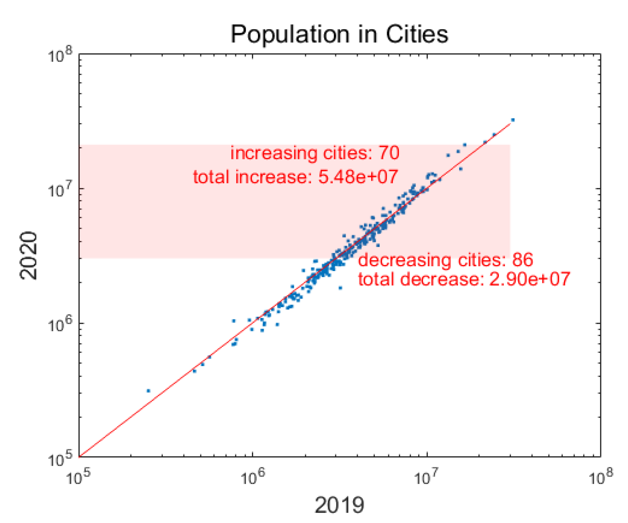
As shown in Figure A8, despite the urban population data for 2019 and 2020 being sourced from different databases, the correlation between the two is high, indicating that the overall data quality is good. Additionally, some notable changes can be observed. For instance, near the second critical point (the red shaded area on the y-axis), although the number of cities with population growth is still lower than those with population decline, the total amount of population increase in this group of cities is relatively large. This suggests that in 2020, population growth was more pronounced in secondary cities rather than the top three cities. The population distribution of cities with populations around 10 million became relatively more even, which in turn led to an increase in . This change slightly lowered the threshold for large cities to surpass the knowledge-spillover barrier.
Figure A8.
Comparison of urban population data for 2019 and 2020 from different databases. Source: 2020 data from the 7th National Population Census (2020), National Bureau of Statistics, China; 2019 data from the “China City Statistical Yearbook”.
Figure A8.
Comparison of urban population data for 2019 and 2020 from different databases. Source: 2020 data from the 7th National Population Census (2020), National Bureau of Statistics, China; 2019 data from the “China City Statistical Yearbook”.
Appendix C.2. Labor Demand of “Knowledge-Spillover” Cities in China
According to the fitting results, the critical thresholds and for transitioning to sub-innovative and super-innovative economies can be obtained. These thresholds help us understand the development paths and labor demands of “knowledge-spillover” cities in China. The calculated results are shown in Table A2. Additionally, based on empirical analysis, the critical points are saddle points, with the Hessian matrix having one positive eigenvalue and one negative eigenvalue.
Table A2.
Calculation results of And (in people)
| Year | ||
|---|---|---|
| 2004 | ||
| 2005 | ||
| 2006 | ||
| 2007 | ||
| 2008 | ||
| 2009 | ||
| 2010 | ||
| 2011 | ||
| 2012 | ||
| 2013 | ||
| 2014 | ||
| 2015 | ||
| 2016 | ||
| 2017 | ||
| 2018 | ||
| 2019 | ||
| 2020 |
Appendix C.3. Comparison with the Optimal City Size
in China is around people, while that in the United States is about people. As has been analyzed in the previous session, in addition to the gap in absolute population (that is, the various and in different countries), this difference mainly comes from the distribution characteristics of city size in different countries, as . In the traditional theory of optimal city size, for a single city, the optimal city size was a typical optimization problem that comprehensively considered economic externality or agglomeration utility, and commuting or rental costs [57,59]; Some scholars expanded the scope of social costs to include environmental protection [17,60], or measured the optimal size of multiple cities in the urban system using the rank-size rule [62].
From the perspective of maximizing the net income of city size, Wang pointed out that the optimal city size in China should be about [64]. Carlino analyzed the relationship between agglomeration economies and increasing returns to scale, and quantified that the optimal city size in the United States is about people [65]. Using Carlino’s method for reference, Jin indicated that the optimal city size of Beijing, Shanghai and Tianjin was around [66]. Of course, when environmental pollution and energy efficiency are considered, the optimal city size is significantly smaller than that in previous research, not exceeding people in China [68]. However, these literature take output as a whole, without analyzing the dependence and influence of changes in output structure on city size.
Using a typical optimal size model for individual cities, it quantifies the optimal city size in China and the United States by analyzing personal income and expenditure [57]. Based on empirical data from 2019, the optimal city size in the United States is people, while that in China is people. Although the optimal size model differs from our method, both approaches yield similar quantitative results.
In the optimal size model, represents the exponent of the relationship between per capita GDP growth and urban population size. Both and describe the population-based scale effect and urban endogenous agglomeration benefits from different perspectives. China has a smaller and a larger (Table A3). A smaller indicates that the population is more concentrated in a few large cities, while a larger suggests that per capita output or personal income is relatively higher in large-scale cities. These factors make China’s optimal city size much larger than that of the United States. Because the population is highly concentrated in a few large cities, the number of cities in China that can cross the second critical transition point is smaller than that in the United States.
The traditional optimal city size model can be used to describe the benefits of urban growth and economies of scale, as well as to analyze problems related to congestion costs. Thus, it serves as a useful supplement and validation for the theory of optimal city size. The employment structure reflects a city’s production characteristics, and the predominance of highly agglomerating industries often means that, for cities of the same size, per capita output will be higher. Therefore, the evolution of employment structure is related to changes in a city’s optimal scale, which can be illustrated through the consistency of results in the two models.
Suppose an urban system with heterogeneous cities, where workers benefit from agglomeration economies that translate into higher outputs. It is proposed that the gross output (per capita) in city i, with population , is given by [57]
where was the exogenous city productivity and represented the benefit of the endogenous agglomeration outside the representative firm. The costs urban dwellers bear consist of commuting costs , and land rents , as
The optimization function is
It uses GDP (per capita) and sales of commodities (per capita) as a proxy for personal income and expenditure , respectively, for the year 2019. The details of the data are shown in Table 1. While data on personal consumption expenditure are only available at the state level, personal income data are available for individual cities. Given the strong correlation between personal income and personal consumption at the state level (Pearson correlation coefficient = 0.9983, sig. = 0.00), it estimates expenditure on personal consumption for each city.
In addition, because the value of a is related to the price unit, it normalizes the per capita output of each city to ensure comparability between China and the United States. Specifically, it adjusts the data so that the mean per capita output is the same for both countries. The results are shown in Table A3. The optimal city size calculated using the optimal city size theory is very close to the second critical point identified by our theoretical model.
Table A3.
Optimum city size of China and the United States in 2019.
| a | ||||
|---|---|---|---|---|
| China | 245.471 | 0.1064 | 0.3528 | 1.13E+07 |
| United States | 131.978 | 0.0994 | 0.3393 | 1.22E+06 |
Appendix C.4. Differences in Cities’ Economic Regions
Because the scaling exponent is influenced by regional development imbalances in China, it divided these cities into groups based on their geographical locations to compare the regional differences in scaling exponents (Table A4).
Table A4.
China’s four major economic regions.
| Region | Provinces |
|---|---|
| Eastern Region | Beijing, Tianjin, Hebei, Shanghai, Jiangsu, Zhejiang, Fujian, Shandong, Guangdong, Hainan, Taiwan, Hong Kong SAR, Macao SAR |
| Central Region | Shanxi, Anhui, Jiangxi, Henan, Hubei, Hunan |
| Western Region | Inner Mongolia Autonomous Region, Guangxi Zhuang Autonomous Region, Chongqing Municipality, Sichuan , Guizhou , Yunnan, Tibet Autonomous Region, Shaanxi, Gansu , Qinghai , Ningxia Hui Autonomous Region, Xinjiang Uygur Autonomous Region |
| Northeast Region | Liaoning, Jilin, Heilongjiang |
| Classification based on the standards of the National Bureau of Statistics of China. | |
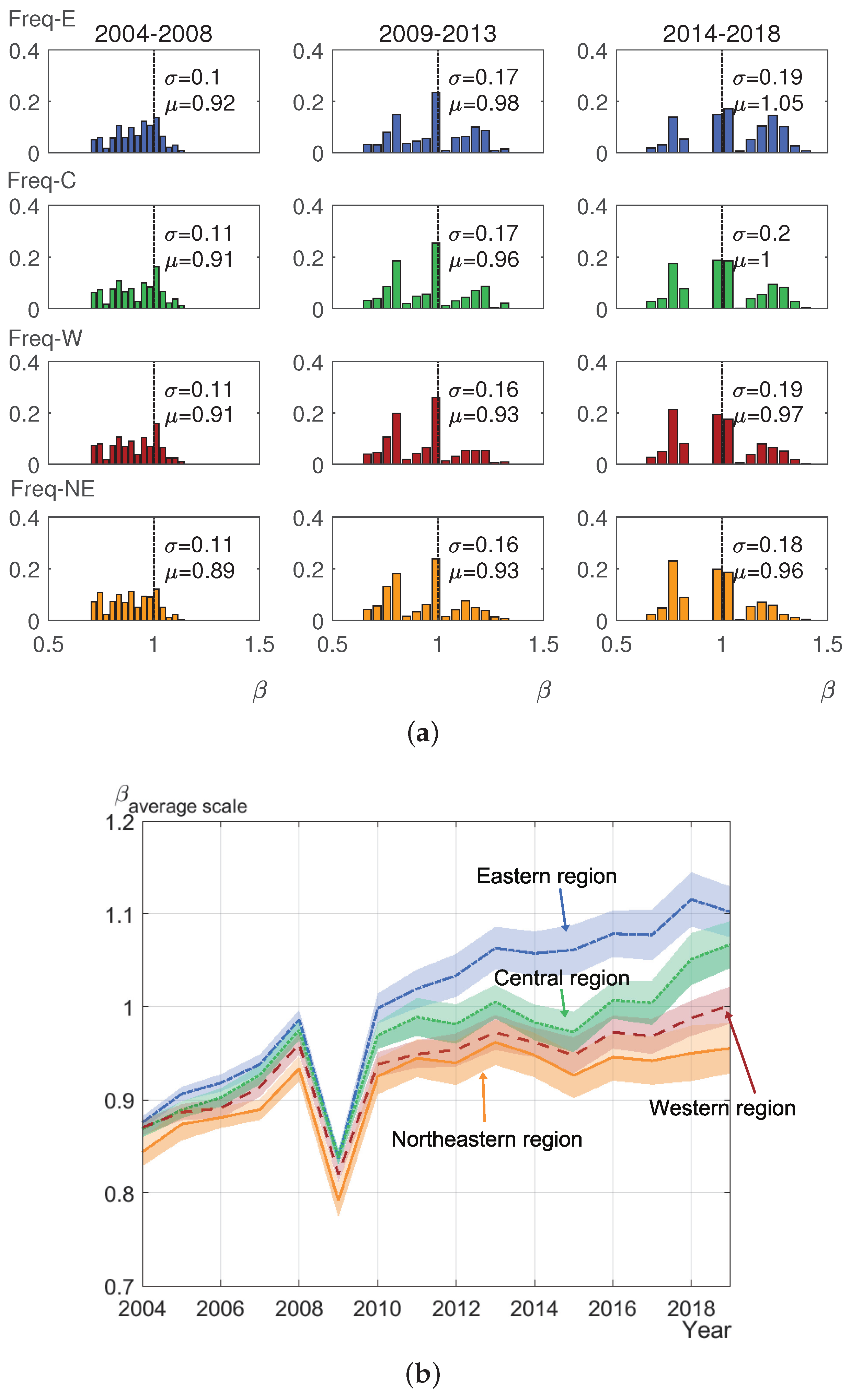
As Figure A9 shows, during a five-year observation period, the scaling characteristics of the four regions generally increased. Notably, the average scaling characteristics of all regions in 2009 decreased sharply. This decline was due to a decrease in employment in 2009 compared to 2007 and 2008, while the urban population continued to grow, resulting in a lower . Although the eastern region had the highest , its growth slowed in subsequent years. In contrast, the central region’s scaling characteristics have accelerated in recent years, indicating that the gap between the central and eastern regions is gradually narrowing. The western region, which followed the central region, had a smaller average scaling characteristic but still showed an upward trend.
Unlike other regions, the scaling characteristics of Northeast China are not only lagging but also exhibit slow growth, indicating that employment in high-agglomerating industries is shrinking. This trend is partly due to the rapid development and construction of the eastern coastal areas, which has caused the industrial center of gravity to shift southward. As a result, emerging industries in economically developed areas have replaced some dominant industries in the northeast. During industrial restructuring in Northeast China, emerging industries started late [79]. Traditional pillar industries occupied significant resources, causing emerging industries to grow slowly and be at a disadvantage in nationwide competition. This situation has led to the relative “absence” of high-agglomerating and emerging industries in Northeast China.
Figure A9.
Differences in the scaling characteristics in different regions. (a) The scaling characteristic distribution (as distribution of with RCA) of all cities in the region is considered every five years. From top to bottom in the figure, they are the eastern region, the central region, the western region, and the northeast region. (b) Different colors represent four economic regions in China. The average scaling characteristic of the city is its average of all characteristic industries (with RCA). The average scaling characteristic of the region is its average of all cities’ scaling characteristics. The shaded part represents the confidence interval of the cities in the region. All calculations are based on data from the same year.
Appendix C.5. The Recapitulation of Industries
In addition to observing the evolution of industries in different cities, it compares the time series of city scale and its related factors over the observed period. These changes are captured in the recapitulation of various industries, as shown in Eq. (A15).
Here, represents the total longitudinal change in employment, while represents the change in employment associated with population size changes (i.e., scaled growth) between the starting year (2004) and the ending year (2019). The regression of on yields the empirical scaled growth coefficient and the nationwide trend . Specifically, denotes the longitudinal scaling effect of population change on employment.
It can obtains the scaling exponents of the cross-sectional change from annual data and the scaling exponents of the vertical change (i.e., the scaled growth coefficient ) from the difference between the beginning and ending years. However, whether these two results are consistent requires further discussion. The recapitulation score quantitatively estimates the consistency between them.
Here, is the scaled growth coefficient, and is the cross-sectional scaling exponent in the t-th year, calculated from Eq. (A1). If population changes are perfectly correlated with employment changes, the scaled growth coefficient is expected to equal the scaling exponent, resulting in a recapitulation score of . Conversely, a recapitulation score of zero indicates that population changes have no effect on employment.
Table A5 shows the recapitulation scores for various industries. Most industries have recapitulation scores higher than 0.5, indicating that their evolutionary paths during urban development are typical and have reference value. However, for industries with low recapitulation scores, such as public facilities, construction, and health, their scaling characteristics should be analyzed on an annual basis rather than focusing solely on average values.
Table A5.
Recapitulation score.
| Industry | Score |
|---|---|
| Manufacturing | 0.75 * |
| Production and supply of electricity, heating, gas, and water | 0.93 * |
| Construction industry | 0.42 |
| Wholesale and retail | 0.68 * |
| Transportation, warehousing, and postal services | 0.83 * |
| Accommodation and catering industry | 0.85 * |
| Information transmission, computing services, and software | 0.67 * |
| Finance | 0.61 * |
| Real estate industry | 0.91 * |
| Rent | 0.83 * |
| Scientific research, technical services, and geological survey | 0.77 * |
| Public facilities management industry | -0.91 |
| Residential services, repair, and other services | 0.73 * |
| Educational services | 0.83 * |
| Health care and social work | 0.42 |
| Culture, sports, and entertainment | 0.82 * |
| Public administration, social security, and social organization | 0.60 * |
| * indicates the industries with . |
References
- Bettencourt, L.M.; West, G. A unified theory of urban living. Nature 2010, 467, 912–913. [Google Scholar] [CrossRef] [PubMed]
- Chen, M.; Zhang, H.; Liu, W.; Zhang, W. The global pattern of urbanization and economic growth: evidence from the last three decades. PloS One 2014, 9, e103799. [Google Scholar] [CrossRef] [PubMed]
- UN, D. World urbanization prospects: The 2014 revision. United Nations Department of Economics and Social Affairs, Population Division: New York, NY, USA 2015, 41. [Google Scholar]
- Balland, P.A.; Jara-Figueroa, C.; Petralia, S.G.; Steijn, M.P.; Rigby, D.L.; Hidalgo, C.A. Complex economic activities concentrate in large cities. Nature Human Behaviour 2020, 4, 248–254. [Google Scholar] [CrossRef]
- Xu, H.; Jiao, M. City size, industrial structure and urbanization quality—A case study of the Yangtze River Delta urban agglomeration in China. Land Use Policy 2021, 111, 105735. [Google Scholar] [CrossRef]
- Zheng, S.; Du, R. How does urban agglomeration integration promote entrepreneurship in China? Evidence from regional human capital spillovers and market integration. Cities 2020, 97, 102529. [Google Scholar] [CrossRef]
- Hong, I.; Frank, M.R.; Rahwan, I.; Jung, W.S.; Youn, H. The universal pathway to innovative urban economies. Science Advances 2020, 6, eaba4934. [Google Scholar] [CrossRef]
- Bettencourt, L.M.; Lobo, J.; Helbing, D.; Kühnert, C.; West, G.B. Growth, innovation, scaling, and the pace of life in cities. Proceedings of the National Academy of Sciences 2007, 104, 7301–7306. [Google Scholar] [CrossRef]
- Bettencourt, L.M. The Origins of Scaling in Cities. Science 2013, 340, 1438–1441. [Google Scholar] [CrossRef]
- Bettencourt, L.M.; Lobo, J.; West, G.B. Why are large cities faster? Universal scaling and self-similarity in urban organization and dynamics. The European Physical Journal B 2008, 63, 285–293. [Google Scholar] [CrossRef]
- Pumain, D.; Paulus, F.; Vacchiani-Marcuzzo, C.; Lobo, J. An evolutionary theory for interpreting urban scaling laws. Cybergeo: European Journal of Geography 2006, 2006, 1–20. [Google Scholar] [CrossRef]
- Youn, H.; Bettencourt, L.; Lobo, J.; Strumsky, D.; Samaniego, H.; West, G. Scaling and universality in urban economic diversification. Journal of the Royal Society Interface 2016, 13, 20150937. [Google Scholar] [CrossRef] [PubMed]
- Misra, S.B. Revisiting Rural Non-farm Sector Employment in India: Trends from 1993-94 to 2023-24. Indian Journal of Human Development 2025, 0, 09737030251322830. [Google Scholar] [CrossRef]
- Ge, P.; Sun, W.; Zhao, Z. Employment structure in China from 1990 to 2015. Journal of Economic Behavior & Organization 2021, 185, 168–190. [Google Scholar]
- Arif, I. Productive knowledge, economic sophistication, and labor share. World Development 2021, 139, 105303. [Google Scholar] [CrossRef]
- Li, X.; Huang, S.; Chen, Q. Analyzing the driving and dragging force in China’s inter-provincial migration flows. International Journal of Modern Physics C 2019, 30, 1940015. [Google Scholar] [CrossRef]
- Chen, Y. The evolution of Zipf’s law indicative of city development. Physica A: Statistical Mechanics and its Applications 2016, 443, 555–567. [Google Scholar] [CrossRef]
- Taylor, J.R. The China dream is an urban dream: Assessing the CPC’s national new-type urbanization plan. Journal of Chinese Political Science 2015, 20, 107–120. [Google Scholar] [CrossRef]
- Ye, X.; Xie, Y. Re-examination of Zipf’s law and urban dynamic in China: a regional approach. The Annals of Regional Science 2012, 49, 135–156. [Google Scholar] [CrossRef]
- Guan, X.; Wei, H.; Lu, S.; Dai, Q.; Su, H. Assessment on the urbanization strategy in China: Achievements, challenges and reflections. Habitat International 2018, 71, 97–109. [Google Scholar] [CrossRef]
- Chen, X.; Du, W. Too big or too small? The threshold effects of city size on regional pollution in China. International Journal of Environmental Research and Public Health 2022, 19, 2184. [Google Scholar] [CrossRef] [PubMed]
- Zhou, Y.; Xu, H.; Wang, Y.; Li, C.; Luo, Q.; Chen, S. Promoting coordinated spatial governance of mega-cities in China via spatial organization of metropolitan areas. Frontiers of Urban and Rural Planning 2024, 2, 1–16. [Google Scholar] [CrossRef]
- Zheng, D.; Dong, S.; Lin, C. The Necessity and Control Strategy of “Medium Density” in Metropolis. Int. Urban Plan 2021, 36, 1–9. [Google Scholar]
- Zipf, G.K. Human behavior and the principle of least effort: An introduction to human ecology; Ravenio Books, 2016.
- Hu, Y.; Connor, D.S.; Stuhlmacher, M.; Peng, J.; Turner Ii, B. More urbanization, more polarization: evidence from two decades of urban expansion in China. npj Urban Sustainability 2024, 4, 33. [Google Scholar] [CrossRef]
- Bee, M.; Riccaboni, M.; Schiavo, S. The size distribution of US cities: Not Pareto, even in the tail. Economics Letters 2013, 120, 232–237. [Google Scholar] [CrossRef]
- Berry, B.J.; Okulicz-Kozaryn, A. The city size distribution debate: Resolution for US urban regions and megalopolitan areas. Cities 2012, 29, S17–S23. [Google Scholar] [CrossRef]
- Li, H.; Wei, Y.D.; Ning, Y. Spatial and temporal evolution of urban systems in China during rapid urbanization. Sustainability 2016, 8, 651. [Google Scholar] [CrossRef]
- Mori, T.; Smith, T.E.; Hsu, W.T. Common power laws for cities and spatial fractal structures. Proceedings of the National Academy of Sciences 2020, 117, 6469–6475. [Google Scholar] [CrossRef]
- Ribeiro, H.V.; Oehlers, M.; Moreno-Monroy, A.I.; Kropp, J.P.; Rybski, D. Association between population distribution and urban GDP scaling. Plos One 2021, 16, e0245771. [Google Scholar] [CrossRef]
- Zhao, S.X.; Guo, N.S.; Li, C.L.K.; Smith, C. Megacities, the world’s largest cities unleashed: major trends and dynamics in contemporary global urban development. World Development 2017, 98, 257–289. [Google Scholar] [CrossRef]
- Friedmann, J. Four theses in the study of China’s urbanization. International Journal of Urban and Regional Research 2006, 30, 440–451. [Google Scholar] [CrossRef]
- Frank, M.R.; Sun, L.; Cebrian, M.; Youn, H.; Rahwan, I. Small cities face greater impact from automation. Journal of the Royal Society Interface 2018, 15, 20170946. [Google Scholar] [CrossRef] [PubMed]
- Bai, X.; Shi, P.; Liu, Y. Society: Realizing China’s urban dream. Nature News 2014, 509, 158. [Google Scholar] [CrossRef] [PubMed]
- Wang, X.R.; Hui, E.C.M.; Choguill, C.; Jia, S.H. The new urbanization policy in China: Which way forward? Habitat International 2015, 47, 279–284. [Google Scholar] [CrossRef]
- Xu, Z.; Zhu, N. City size distribution in China: are large cities dominant? Urban Studies 2009, 46, 2159–2185. [Google Scholar] [CrossRef]
- Gao, B.; Huang, Q.; He, C.; Dou, Y. Similarities and differences of city-size distributions in three main urban agglomerations of China from 1992 to 2015: A comparative study based on nighttime light data. Journal of Geographical Sciences 2017, 27, 533–545. [Google Scholar] [CrossRef]
- Fang, L.; Li, P.; Song, S. China’s development policies and city size distribution: An analysis based on Zipf’s law. Urban Studies 2017, 54, 2818–2834. [Google Scholar] [CrossRef]
- Cai, E.; Zhang, S.; Chen, W.; Li, L. Spatio–temporal dynamics and human–land synergistic relationship of urban expansion in Chinese megacities. Heliyon 2023, 9, e19872. [Google Scholar] [CrossRef]
- ECNS. 17 Chinese cities have a population of over 10 million in 2021. https://www.ecns.cn/news/cns-wire/2022-05-26/detail-ihaytawr8118445.shtml, 2022. Accessed: 2025-05-21.
- Liesner, H. The European Common Market and British Industry. The Economic Journal 1958, 68, 302–316. [Google Scholar] [CrossRef]
- Levy, M. Gibrat’s Law for (All) Cities: Comment. American Economic Review 2009, 99, 1672–1675. [Google Scholar] [CrossRef]
- Deng, Z.; Fan, H. Study on the law of urban population size distribution in China. Chinese Journal of Population Science 2016, 000, 48–60. [Google Scholar]
- Chen, D.; Yan, Z.; Wang, W. Urban population size, industrial agglomeration model and urban innovation: empirical evidence from 271 cities at prefecture level and above. Chinese Journal of Population Science 2020, 34, 27–40. [Google Scholar]
- Dong, K. Research on Urban Power Law Distribution and Urban Allometric Scaling. PhD thesis, University of Chinese Academy of Sciences, 2019.
- Blank, A.; Solomon, S. Power laws in cities population, financial markets and internet sites (scaling in systems with a variable number of components). Physica A: Statistical Mechanics and its Applications 2000, 287, 279–288. [Google Scholar] [CrossRef]
- Gabaix, X. Power laws in economics: An introduction. Journal of Economic Perspectives 2016, 30, 185–206. [Google Scholar] [CrossRef]
- González-Val, R.; Lanaspa, L.; Sanz-Gracia, F. New evidence on Gibrat’s law for cities. Urban Studies 2014, 51, 93–115. [Google Scholar] [CrossRef]
- Lalanne, A. Zipf’s law and Canadian urban growth. Urban Studies 2014, 51, 1725–1740. [Google Scholar] [CrossRef]
- Wei, S.; Sun, N.; Jiang, Y. Applicability of Zipf’s law and Gibrat’s law in urban size distribution in China. The Journal of World Economy 2018, 000, 96–120. [Google Scholar]
- Eeckhout, J. Gibrat’s Law for (All) Cities. American Economic Review 2004, 94, 1429–1451. [Google Scholar] [CrossRef]
- Malevergne, Y.; Pisarenko, V.; Sornette, D. Testing the Pareto against the lognormal distributions with the uniformly most powerful unbiased test applied to the distribution of cities. Physical Review E 2011, 83, 036111. [Google Scholar] [CrossRef]
- Rabinowitz, P.H.; et al. Minimax methods in critical point theory with applications to differential equations; Number 65, American Mathematical Soc., 1986.
- Frank, M.R.; Sun, L.; Cebrian, M.; Youn, H.; Rahwan, I. Small cities face greater impact from automation. Journal of the Royal Society Interface 2018, 15, 20170946. [Google Scholar] [CrossRef]
- Michaels, G.; Rauch, J.; Redding, S.J. Task Specialization in U.S. Cities from 1880 to 2000. Journal of the European Economic Association 2019, 17, 754–798. [Google Scholar] [CrossRef]
- Balland, P.A.; Jara-Figueroa, C.; Petralia, S.G.; Steijn, M.P.; Hidalgo, C.A. Complex economic activities concentrate in large cities. Nature Human Behaviour 2020, 4, 1–7. [Google Scholar] [CrossRef] [PubMed]
- Albouy, D.; Behrens, K.; Robert-Nicoud, F.; Seegert, N. The optimal distribution of population across cities. Journal of Urban Economics 2019, 110, 102–113. [Google Scholar] [CrossRef]
- Henderson, J.V. Optimum city size: The external diseconomy question. Journal of Political Economy 1974, 82, 373–388. [Google Scholar] [CrossRef]
- Capello, R.; Camagni, R. Beyond optimal city size: an evaluation of alternative urban growth patterns. Urban Studies 2000, 37, 1479–1496. [Google Scholar] [CrossRef]
- Mizutani, F.; Tanaka, T.; Nakayama, N. Estimation of optimal metropolitan size in Japan with consideration of social costs. Empirical Economics 2015, 48, 1713–1730. [Google Scholar] [CrossRef]
- Giesen, K.; Südekum, J. Zipf’s law for cities in the regions and the country. Journal of Economic Geography 2011, 11, 667–686. [Google Scholar] [CrossRef]
- Jiang, B.; Yin, J.; Liu, Q. Zipf’s law for all the natural cities around the world. International Journal of Geographical Information Science 2015, 29, 498–522. [Google Scholar] [CrossRef]
- Verbavatz, V.; Barthelemy, M. The growth equation of cities. Nature 2020, 587, 397–401. [Google Scholar] [CrossRef]
- Wang, X. Urbanization Path and City Scale in China: An Economic Analysis. Economic Research Journal 2010, 10, 20–32. [Google Scholar]
- Carlino, G. Manufacturing agglomeration economies as returns to scale: A production function approach 1982. 50, 95–108.
- Jin, X. Theories on the Optimum Scales of Cities and Empirical Study: Taking the Example of the Three Municipalities. Shanghai Economic Review 2004, 2004, 35–43. [Google Scholar] [CrossRef]
- Zhang, Y. The Empirical Study of Optimal City Size in China: The Perspective of Economic Growth. Shanghai Economic Review 2009, 8. [Google Scholar]
- Jie, Z.; Yang, X. Optimal city size in China: An extended empirical study from the perspective of energy consumption. China City Planning Review 2017, 26, 22–29. [Google Scholar]
- United States Census Bureau. Metropolitan and Micropolitan Statistical Areas Population Totals and Components of Change: 2010-2019. Technical report, Population Division, United States Census Bureau, Washington, DC, 2020.
- Sun, W.; Jones, J.; Gamber, M. A Turning Point for China’s Population: No Child and Long Illness. Aging and Disease 2023, 14, 1950–1952. [Google Scholar] [CrossRef] [PubMed]
- Wang, P. Population Decline Narrows, Population Quality Continues to Improve. https://www.stats.gov.cn/sj/sjjd/202501/t20250117_1958337.html, 2025. National Bureau of Statistics of China.
- United Nations. World Population Aging. Technical report, Department of Economic and Social Affairs, Population Division, New York, NY, 2017.
- Liang, J. Prospects for Chinas drive for innovation: from the perspective of demographics. In China and the West; Edward Elgar Publishing, 2021; pp. 135–147.
- Yu, X.; Yi, T. Analysis on the Influencing Mechanism of Population Agglomeration, Industry Agglomeration and Innovation Agglomeration in Chinese Megacities. Commercial Research 2020, 62, 145–152. [Google Scholar]
- Zipf, G.K. Human Behavior and the Principle of Least Effort: An Introduction to Human Ecology; Ravenio Books: London, 2016. [Google Scholar]
- Jiang, B.; Jia, T. Zipf’s law for all the natural cities in the United States: a geospatial perspective. International Journal of Geographical Information Science 2011, 25, 1269–1281. [Google Scholar] [CrossRef]
- Hidalgo, C.A.; Hausmann, R. The building blocks of economic complexity. Proc Nat Acad Sci USA 2009, 106, 10570–10575. [Google Scholar] [CrossRef]
- Hausmann, R.; Hidalgo, C.A. The network structure of economic output. Journal of Economic Growth 2011, 16, 309–342. [Google Scholar] [CrossRef]
- Zhao, R.; Wang, Y. Analysis on the causes of frequent economic recession in Northeast China – the change from "industry absence" to "system solidification". Social Science Front 2017, 000, 48–57. [Google Scholar]
| 1 | Urban areas are ranked by population size in descending order. The population of the urban area ranked r is proportional to . For example, the largest urban area has twice the population of the second-largest urban area, three times that of the third-largest urban area, and so on. Although Zipf’s law is not expressed as a probability density function, it also indicates that the population of top-ranked urban areas is much larger than that of lower-ranked urban areas. |
| 2 | The resident population can fully reflect the mobility characteristics of the current Chinese population and accurately depict the urbanization level based on the resident population standard. |
| 3 | According to the spirit of the 28th executive meeting of the State Council, the National Bureau of Statistics issued the Notice on Improving and Standardizing Regional GDP Accounting on January 6, 2004, requiring provinces, autonomous regions, and municipalities to uniformly calculate per capita GDP using the resident population (i.e., the registered population minus the outflow population of more than half a year plus the inflow population). |
| 4 | Specifically, 16 cities lack GRP data for several years, which poses problems for obtaining permanent resident population data (Sansha, Zhangzhou, Bijie, Zunyi, Tongren, Lasa, Rikaze, Changdu, Linzhi, Shannan, Naqu, Longnan, Haidong, Zhongwei, Tulufan, Hami); 2 cities lack all employment population data of certain industries (Ziyang and Hengshui), and these 18 cities were excluded from the analysis. Additionally, Laiwu was merged into Jinan in January 2019, and it was retained in the analysis to maintain consistency |
| 5 | As there are many empirical models of the optimal city size, which cannot be tested one by one, we only take a representative model as an example to compare such methods with the empirical results of our study. |
Disclaimer/Publisher’s Note: The statements, opinions and data contained in all publications are solely those of the individual author(s) and contributor(s) and not of MDPI and/or the editor(s). MDPI and/or the editor(s) disclaim responsibility for any injury to people or property resulting from any ideas, methods, instructions or products referred to in the content. |
© 2025 by the authors. Licensee MDPI, Basel, Switzerland. This article is an open access article distributed under the terms and conditions of the Creative Commons Attribution (CC BY) license (https://creativecommons.org/licenses/by/4.0/).
Copyright: This open access article is published under a Creative Commons CC BY 4.0 license, which permit the free download, distribution, and reuse, provided that the author and preprint are cited in any reuse.


