
Submitted:
03 June 2025
Posted:
03 June 2025
You are already at the latest version
Abstract
In this study, a procedure based on Phase-locked Proper Orthogonal Decomposition (PPOD) was applied to Large Eddy Simulations (LES) of two low-pressure turbine blades operating with unsteady inflow. This decomposition allows the inspection of the effect of blade loading on loss generation mechanisms, especially focusing on their variation throughout the incoming wake period. After sorting snapshots based on their phase within the wake cycle using temporal POD coefficients associated with wake migration, POD was reapplied to each sub-ensemble of snapshots at a given phase, providing an optimal representation of the dynamics at fixed wake locations. This highlighted the effects of migration, bowing, tilting, and reorientation of the incoming wake filaments, as well as the breakup of streaky structures in the blade boundary layer and the formation of Von Karman vortices at the blade trailing edge. PPOD offered the opportunity to observe how all these processes are modulated and change throughout the wake period. The comparison between the two analyzed blades showed that overall loss generation follows similar temporal patterns during the wake passing cycle, increasing with the propagation of the upstream wake and reaching its maximum value when the wake is in the peak suction position. According to the specific blade loading distribution, the production of TKE was observed in different regions of the computational domain. The described procedure may contribute to the development of advanced design processes based on physically-informed strategies.
Keywords:
turbomachinery
; wake-boundary layer interaction
; losses
; optimization
1. Introduction
The efficiency and performance of aircraft engines are pivotal in determining overall flight capabilities and fuel consumption. Among the numerous components that contribute to engine efficiency, turbine blades play a critical role by converting the internal energy of high-velocity gas into mechanical work. The pursuit of enhanced turbine efficiency has driven the development and refinement of methodologies for assessing the losses incurred by turbine blades during operation. Based on Denton’s work [1], many subsequent studies have highlighted how losses associated with the flow around turbine blades are influenced by various geometric and operational parameters, including profile curvature, pitch-to-chord ratio, Reynolds number and Mach number [2]. In particular, the unsteadiness of the flow, due to the fluid-dynamic interaction between stator and rotor blades, plays a fundamental role in the generation of losses, as reported in [3,4,5,9,10]. Nowadays, the upstream wake effect on boundary layer development is widely recognized as a large and small scale turbulent interaction which forces boundary layer transition, as reported by Shulte and Hodson [6], Wu et al. [7] and Lengani et al. [8]. However, the complete understanding of this and other mechanisms leading to loss production is far from being achieved and the fine inspection and quantification of the various contributions to the overall loss remain difficult tasks. In recent years, detailed high fidelity simulations, such as Large Eddy Simulations (LES) and Direct Numerical Simulations (DNS), have become common practice for the study of unsteady flows in turbomachinery. As noted by Sandberg and Michelassi [11], experimental tests often face the limitation of examining, albeit in detail, phenomena occurring in a restricted region of the fluid domain. In contrast, numerical simulations enable the extraction of localized information throughout the entire computational domain and provide deep insight into the complex flow dynamics responsible for loss production. The availability of vast CFD databases has driven research towards the development of innovative data analysis techniques, capable of extracting key information about the flow characteristics. In this context, the dimensionality reduction of the dataset achieved through modal decomposition techniques represents a tool of great potential. Among these techniques, the Proper Orthogonal Decomposition (POD), introduced by Lumley in 1967 [12], is now established as a mature tool for identifying various dynamics driving complex turbulent flows and related loss production mechanisms [13,16,19,20]. As reported in Russo et al. [21], Dellacasagrande et al. [18] and Lengani et al. [17], POD can be used to re-formulate the total pressure transport equation in the Reynolds average sense to highlight the contribution to loss generation of each mode (i.e., dynamical feature), pinpointing the distinct sources of losses. While this procedure allows the identification of their spatial location within the computational domain, it does not provide any additional information on their temporal occurrence within the wake passing period. In this paper, LES data of two high-loaded LPT cascades operating under unsteady inflow conditions have been analyzed using an advanced post-processing procedure based on a Phase-locked POD (PPOD) technique. The PPOD method involves sorting the snapshots based on their temporal occurrence relative to a reference phase of the wake passage cycle. To this end, the classical formulation of POD has been applied to the original dataset and the first two temporal eigenvectors have been exploited to assign every snapshot to the corresponding relative phase, similarly to what is described in Oudheusden et al. and Perrin et al. [14,29]. POD has then been reapplied to the sorted snapshots, performing a modal decomposition of the flow around the blade at a fixed phase. The procedure allowed the inspection of the effect of blade loading on loss generation mechanisms associated with upstream wake and boundary layer interaction and the variation of the related events throughout the incoming wake period. Following the assumptions described in detail in this work, the evaluation of the production of turbulent kinetic energy, which can be reformulated as the sum of products between POD modes, was selected as loss metric. This quantity was integrated, for every single phase, over different regions of the computational domain. This allowed for a clear identification of the temporal and spatial contribution in terms of entropy production due to a specific coherent flow structure. Comparison of the results obtained for the two different blade profiles enabled a fine interpretation of the effects of the loading distribution on loss generation. The paper is organized as follows: in Section 2 the numerical method, the geometrical configuration and the flow parameters are described; in Section 3 the basic equations are presented; in Section 4 the PPOD-based procedure for the time, space and dynamical splitting of loss sources is described in detail. Section 5 is divided into two parts: in SubSection 5.1 the overall performances of the two profiles are described and compared as deduced from LES results; in SubSection 5.2 results from PPOD are described in order to clearly identify the dynamics acting in the different regions of the two LP turbine passages for the most significant phases of the wake passing cycle.
2. Large Eddy Simulation
The dataset used in this study was derived from Large Eddy Simulations conducted using the commercial FV software STAR-CCM+, employing a segregated flow model with bounded-central differencing. A second-order implicit backward differentiation scheme was applied for the time derivative, and the WALE model [22] was chosen for the subgrid-scale modeling, combined with the STAR-CCM+ Synthetic Eddy Model (SEM) [23] to generate turbulence at the domain inlet. Given the low Mach number of the selected conditions, the simulations were performed assuming an incompressible flow regime. To assess the profile’s performance in an environment that closely replicates real low-pressure turbines, a stage-like setup was developed. As depicted in Figure 1, the computational domain comprises a 2D repeating stage with a degree of reaction of 0.5, where profiles are identical between adjacent rows. Each of them operates under similar conditions within their respective frames. Specifically, the original rotor profile is duplicated and mirrored to create the vane profile. This design allows for the study of significant unsteady phenomena in LPTs, such as wake-blade interaction, enabling a comprehensive evaluation of the profile’s performance.
The mesh used for the simulations is a 2D-extruded polyhedral grid extending approximately for 25% of the axial chord in the span-wise direction and consisting of around 25 million cells. The mesh was refined to ensure and across the profile surfaces. In the free-stream region, the computational grid was designed with a target cell size approximately ten times the local Kolmogorov length scale, as estimated from previous RANS computations. The adequacy of the grid resolution in the free stream was later reassessed based on numerical results, using Pope’s criterion M [36] — which represents the ratio of modeled TKE (subgrid-scale contribution) to total TKE (the sum of subgrid and resolved components). As shown in Figure 2, alongside the normalized turbulent kinetic energy (), the distribution of M indicates that with the adopted grid, the modeled turbulent kinetic energy remains below 20% throughout the entire computational domain, even in regions of highest turbulence intensity. A preliminary URANS calculation was conducted to optimize the mesh size and its mean-flow solution was used as the initial condition for the LES. The time step was chosen to maintain a CFL number close to 1 in the area of interest, resulting in 500 samples per blade-passing period. After the LES initialization, four flow-through times (FTTs) were simulated to fully develop the turbulent flow field before the start of data collection, allowing time-averaged results to be quickly and independently processed. It is important to note that the current numerical setup (mesh size, time step, etc.) was selected based on a prior sensitivity analysis on similar test cases [18]. Instantaneous data were collected over a total of eight blade-passing periods, but only one every tenth time step was written to disk, resulting in a total of 400 snapshots for each blade. Time-averaged quantities were monitored to verify the statistical convergence of the mean solution and were post-processed to obtain blade performance metrics, which were then compared with those obtained through PPOD analysis. Table 1 provides the parameters of the current simulations for the two tested profiles, including the Reynolds number (based on axial chord length), flow coefficient , Strouhal number, and the non-dimensional axial gap (AG) between rotor and vane rows.
The overall accuracy of LES calculations is verified by the comparison between the loss coefficients directly computed from LES data and the loss coefficients evaluated through an experimental investigation campaign on the two different profiles, as reported in Table 2. Experimental testing has been performed in a blow-down wind tunnel installed at the Aerodynamics and Turbomachinery Laboratory of the University of Genova. For both geometries, a 7-blade large-scale planar cascade was adopted to assess profile losses through the acquisition of upstream and downstream total pressure signals using a Kiel probe. The experimental setup of the test section is analogous to that reported in [34], ensuring an accuracy in evaluating the total pressure loss coefficient of ±2%.
3. Fundamental Equations
Datasets obtained from LES calculations were post-processed following a local loss evaluation approach. The technique is usually exploited in high-fidelity numerical simulations, where local evaluation is made possible by having access to the instantaneous spatial distribution of both the pressure and velocity fields. When integrated over the computational domain, opportunely selected quantities can also provide a global loss assessment. Thanks to the availability of data, the overall loss magnitude can be obtained by a volume integration of the stagnation pressure substantial derivative. The time-average operator can be applied prior to or after spatial integration, due to their linearity. Thus, the non-dimensional loss metric can be computed as:
where is the volume of the domain, is the volumetric flow rate through it, and is a reference dynamic pressure. Indeed, by mean of the Reynolds’ transport theorem, the spatial integration of the time-averaged substantial derivative can be rewritten as the total pressure flux at the boundaries of the volume . This operation is equivalent to what is done empirically, where losses are typically evaluated through a coefficient of total pressure (temporally or mass averaged), assuming certain hypotheses are met.
Further inspecting and expanding the integrand in equation (1) for an incompressible flow, we obtain:
where the terms identified by the curly bracket represent what is actually measured during experimental tests, thus serving as a precise tool for evaluating losses if the remaining diffusive terms are negligible [24].
The material derivative of the time-mean total pressure can be explicitly expressed as the sum of the transport equation for a pseudo-stagnation pressure of the fluid (including only the mean dynamic pressure) and the TKE transport equation:
By substituting the sum of equations (3) and (4) into equation (2) and considering an adiabatic flow with no exchange of work, the following result is obtained:
Therefore, our goal is to compute the sum of the mean flow viscous dissipation and the viscous dissipation due to turbulence. The latter, in the case of turbulence in equilibrium and negligible or null diffusion terms in equation (4), is equal to the production of turbulent kinetic energy .
Hence, the evaluation of the time-averaged substantial derivative of the total pressure (5) can be obtained through the following equation:
As detailed in a previous work of the authors [21], the equality between the production and dissipation of TKE holds true if the turbulent kinetic energy flux across the domain is overall negligible. Using TKE production as a metric for loss estimation allows us to exploit the properties of POD to rank flow structures based on their contribution to TKE. Conversely, when POD is applied to TKE dissipation, the contribution to entropy production is distributed across a large number of high-order modes, making the identification of dominant structures less straightforward.
4. Data Processing
As previously mentioned, Proper Orthogonal Decomposition (POD) can be exploited to split the contribution of individual flow dynamics to the turbulent kinetic energy production term. This allows for a statistical representation of the turbulence-related loss sources and their spatial locations, but does not provide information on the temporal sequence of turbulent events. The presented PPOD method allows for the splitting and identification of the distinct sources of losses for each phase of the wake passing cycle, providing new perspective for the optimization of the efficiency of modern LPT blades.
The starting point of this procedure is applying the snapshots POD method, as proposed by Sirovich [25], to the fluctuating velocity components. The POD generates two complete orthogonal bases, namely the POD modes () and the related eigenvectors (), which retain the mode dynamics. The POD modes are ranked based on the turbulent kinetic energy associated with each of them. For the analyzed cases, the first two modes obtained from the application of POD to both datasets are representative of the wake evolution in the inter-blade channel. For instance, Figure 3 presents a three-dimensional view of the isosurfaces of the first POD mode, normalized with a reference velocity , for both the profiles. Maximum value of both the first POD modes is around 10% of the reference velocity, as observed in [30]. The correlation between leading modes and wake dynamics can also be observed in the corresponding temporal eigenvectors: when plotted against a temporal coordinate, they exhibit a periodic behavior at the wake passing frequency. Therefore, the first two eigenvectors of each dataset can be used to sort the snapshots based on their relative position within the wake cycle. Further details are provided by Lengani et al. [30], where a similar procedure was applied to PIV data. In this work, the CFD-based results allowed the exploitation of the phase shift between the first two eigenvectors, enabling a robust temporal assignment based on corresponding angular phases. In particular, the angular phase of snapshot at time can be obtained as:
Angular bins with a 36° extension were defined to group snapshots based on the associated angular phase value. The spread of angular phase bins for each wake passage period was arranged to assign an equal number of snapshots for each phase. In particular, for each one of them, around 40 corresponding snapshots were combined to form a single phase subset. Since the complete dataset for a single blade profile consists of 400 snapshots, 10 wake cycle sectors were derived. A simplified diagram of the sorting procedure is provided in Figure 4.
The procedure concludes with the application of POD to each phase-locked ensemble of data (accounting for around 40 snapshots each). The resulting number of snapshots per period ensured that the PPOD procedure met the convergence criteria presented in [35]. Specifically, the PPOD modes obtained were compared with those from a case where the number of snapshots per phase was halved. The cross-correlation between the most significant modes of the two configurations was always greater than 0.87. The bi-orthogonality of the POD modes and eigenvectors allows the expression of Reynolds stresses as the product of the modes of the different fluctuating velocity components:
From which:
Observing Equation (9), it is evident that for , we obtain the trace of the tensor , which is twice the total turbulent kinetic energy corresponding to the selected modes. Equation (10) shows how each spatial POD mode contributes to the turbulent kinetic energy production in the domain of interest.
The considerable size of the dataset at hand required the parallelization of operations for computing Proper Orthogonal Decomposition on HPCs. The procedure is similar to the one described in Biassoni et al. [26], with appropriate adjustments to work with a series of independent, small-sized datasets.
A more in-depth examination of the contribution of various flow features to overall profile losses was pursued by evaluating the volume integral of equation (6) within sub-regions, namely, the core flow, the boundary layer (BL), and the mixing region downstream of the vane trailing edge, as depicted in Figure 5. This approach joins the methodology employed by Russo et al. [21], Dellacasagrande et al. [18], Lengani et al. [17] and Leggett et al. [27]. The analysis of the PPOD-based loss distribution in the boundary layer, the mixing region, and the core flow further elucidated the contribution of each coherent flow structure to the overall total pressure losses for the different phases [28].
5. Results and Discussion
5.1. Overall Performance Analysis
Figure 6 illustrates the time-averaged pressure coefficient () normalized with the peak suction value of profile "1", as a function of the dimensionless axial coordinate, for the two analyzed cascades. The pressure coefficient is defined as follows:
where the subscript "t" denotes that the variable is calculated at the stagnation point, while the subscripts "1" and "2" indicate the upstream and downstream sections of the computational domain, respectively.
As can be observed in Figure 6, profile "1" is a strongly aft-loaded profile, with the peak suction position located at 83% of the axial chord. On the other hand, profile "2", albeit still aft-loaded, exhibits a peak suction location that is shifted closer to the leading edge, occurring at 74% of the axial chord. Moreover, profile "2" has a higher loading. Based on these considerations, profiles "1" and "2" will be referred to as Aft-Loaded (AL) and High-Loaded (HL) profile, respectively. The upstream shift of the point of maximum flow velocity for the HL profile allows for a more gradual deceleration in the rear portion of the suction side: despite a higher overall diffusion, a 10% reduction in local diffusion rate with respect to the AL profile is observed, with the blue curve having a greater maximum negative slope than the red curve near the trailing edge. Furthermore, the higher loading of the HL profile allows for a greater flow acceleration in the front part of the suction side.
The global loss coefficient, defined as the normalized inlet-outlet difference in area-averaged total pressure, was computed from LES data to validate the results obtained from the approach introduced in Section 3. The isoentropic downstream velocity-based dynamic pressure was selected as the normalization factor. Despite having a higher blade loading, the HL profile is more efficient than the AL profile, the latter exhibiting a loss coefficient approximately 15% higher.
A POD-based post-processing procedure, analogous to the one presented in [21], has been adopted to identify the main viscous and turbulent phenomena that differentiate the performance of the two profiles. Figure 7 and Figure 8 show the cumulative distributions of the loss coefficients, in both cases normalized with the global loss coefficient of the AL profile. These curves were obtained by integrating the right-hand side terms of Equation (6). These terms have been decomposed in the POD framework, as outlined in Section 4, and then integrated over the different flow regions of the computational domain depicted in Figure 5. In these plots the mean flow viscous dissipation is reported as the baseline loss level cutting the ordinate axis, since it cannot be POD decomposed (i.e. it is related only to mean flow properties), while the contribution of each mode to the remaining term has been cumulatively summed. As expected, both the profiles feature viscous losses mainly concentrated in the blade boundary layer.
Specifically, for the AL profile (Figure 7), the extended accelerated front section of the profile results in significant viscous losses in the accelerating suction side boundary layer (red curve). In this region, as well as in the pressure side boundary layer (violet curve), turbulent structures identified by POD modes do not produce additional losses, as the boundary layers in these portions of the blade remain in a laminar state. This is reflected in the curves showing minimal dependence on mode order (curves are horizontal). In contrast, turbulence-induced losses are more pronounced in the rear part of the suction side where flow diffusion and BL transition occur. In fact, in this area, the contribution to losses increases with mode number (yellow curve). Additionally, considerable losses are observed in the wake region (cyan curve) downstream of the trailing edge. This is due to the intense vortex shedding and related break-up process in the wake, which stems from the strong deceleration of the flow in the rear suction side, where the local diffusion rate reaches very high values. Finally, turbulent production in the core flow region significantly contributes to the total losses (green curve). Both the incoming wake-related modes (i.e. the first modes) and finer scale structures (i.e. higher order modes) induce losses within the passage. This effect is likely due to the moderate acceleration imposed by the blade loading in the early part of the vane passage. As shown in Simoni et al. [31], the insufficient flow acceleration in the initial portion of the blade does not inhibit turbulent production caused by wake bowing and tilting processes. This ultimately leads to an increase in total pressure losses.
Referring now to the HL profile (Figure 8), the cumulative curves of total dissipation show a significant improvement in overall performance with respect to the AL profile. The overall loss (blue curve for the entire set of modes) is approximately 85% of the AL profile value. The most significant contribution to loss production comes from the decelerating suction side region (yellow curve). Losses due to wake migration into the passage region (green curve) are also reduced, thanks to the increased acceleration imposed on the flow by the blade loading. Similarly, viscous dissipation in the accelerating part of the suction side boundary layer (red curve) is lower with respect to the AL profile.
All of this information enhances our understanding of the mechanisms leading to loss generation. A deeper insight can be obtained by examining the phase of the wake passing cycle during which losses are produced.
5.2. Loss Distribution Within Wake Passing Cycle
As described in Section 4, the application of the PPOD procedure results in a modal decomposition of the flow dynamics for a given position of the wake within the inter-blade channel. For instance, Figure 9 shows the contour plots of the HL profile’s first PPOD mode for the stream-parallel velocity component , normalized with , for two different phases capturing the migration of the upstream wake along the blade suction side. Mode streamlines are overlaid on the plots for the portion of the channel above the suction side. As can be observed, the first mode of each phase provides a filtered (or phase-averaged) view of the flow field for each relative position of the wake (wake centerline is schematically represented by a red dashed line).
The figure illustrates the temporal evolution of the main large scale coherent structures generated by the relative motion of the wake within the inter-blade passage from phase 2 to phase 7. Streamlines highlight the formation of the so-called "negative-jet" structure, emphasized by the strongly negative streamwise velocity zone (dark gray flood in the contour plots). The momentum transfer associated with the wake velocity defect generates a jet which, around the wake centerline, directs toward the blade suction side. This jet splits into two branches, forming two distinct large-scale counter-rotating vortices at the leading and trailing edges of the wake, as known from previous literature results. In the figure, these structures are referred to as "Q1" and "Q2" vortices. The negative jet is known to play a key role in the mechanism of wake-induced boundary layer transition. As the wake convects over the boundary layer separation point, the wall-normal component of the negative jet distorts the shear layer, which is inherently unstable. This interaction triggers an inviscid Kelvin-Helmholtz roll-up, where the resulting vortex moves at half the freestream velocity. The wake, traveling at the freestream speed, advances ahead of the roll-up and further disturbs the separated shear layer downstream, leading to the formation of additional roll-up vortices that quickly break down into turbulence.
To identify the phases of the wake passage cycle during which these wake-related events induce the largest losses, we analyze the contribution to losses limited to the production of TKE () by defining a loss coefficient . This coefficient was calculated by integrating, at a fixed phase, the term from equation 6 across the five different sub-regions of the computational domain. Figure 10 and Figure 11 show the bar plots of normalized by the overall loss coefficient obtained for the AL profile, such that the cumulative sum of the bar plots across all phases represents the percentage loss, excluding the viscous term contribution.
For both blades, the phase characterized by the minimum turbulence-related loss is phase 2, which corresponds to the wake located close to the leading edge of the blade (see fig. Figure 9). Here, turbulent production is primarily concentrated in the passage region (green area in Figure 10 for phase 2). As the wake centerline moves towards the trailing edge of the profile, losses increase and become dominated by events in the decelerating region of the blade suction side and within the profile’s wake, with the passage region no longer being the area characterized by the maximum turbulent production. Maximum loss for both profiles is observed at phase 7, even though the spatial flow regions where these occur differ significantly between the two profiles. For the AL profile, the largest contribution to the total loss is attributed to the wake region (cyan sector), while for the HL profile, higher losses are observed in the decelerated boundary layer (yellow sector).
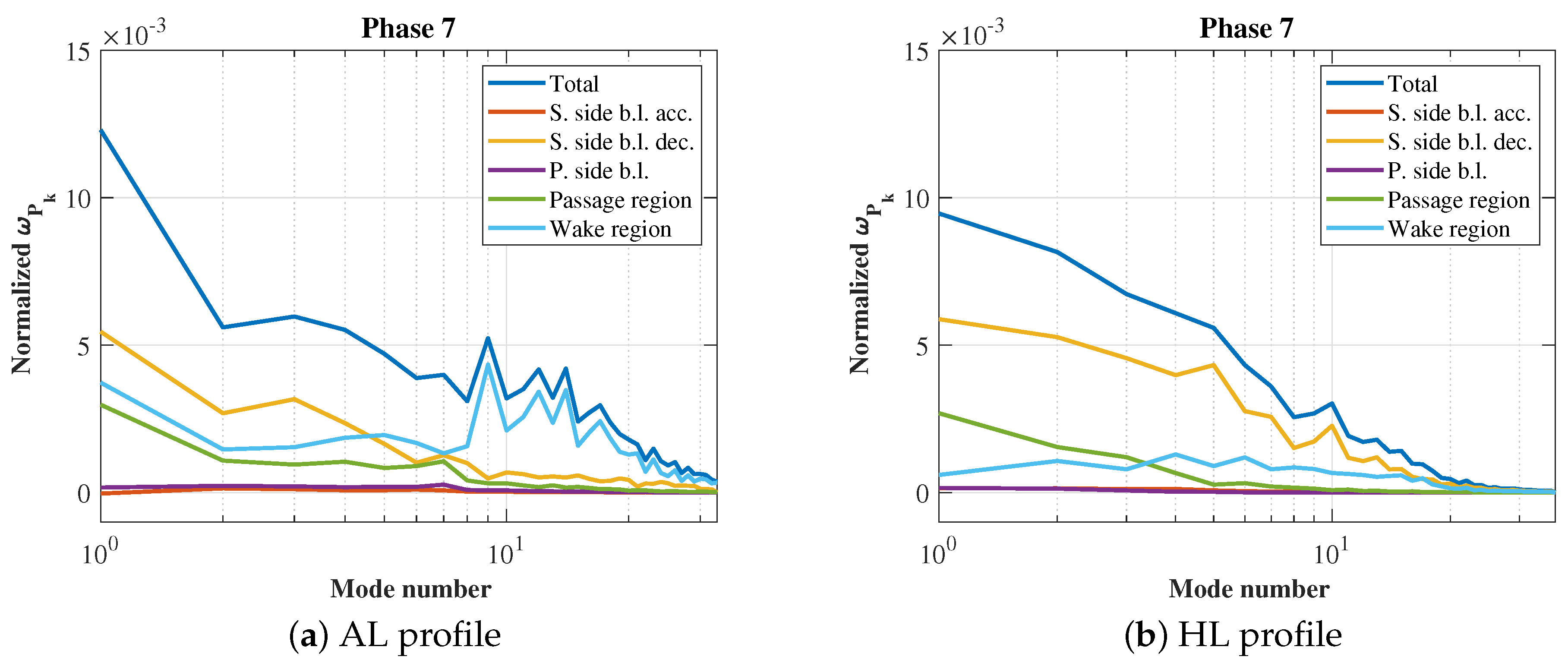
These observations are reflected in the plots of normalized as a function of the PPOD mode index at a fixed phase. Figures and show this trend for the phase characterized by the lowest turbulent production (phase 2) for the AL and HL profiles, respectively. As can be observed, in both cases, the most significant contribution to turbulent kinetic energy production is primarily associated with the low-order modes (i.e., for mode indices smaller than 10), which predominantly act in the passage region (green curve), with a minor additional contribution in the decelerating part of the boundary layer (yellow curve). As previously observed in Figure 9, at this phase the upstream wake is located near the leading edge of the cascade, thus the momentum impingement effects on the rear suction side are limited. The boundary layer is stabilized by the acceleration of the flow imposed by the blade loading, which keeps its laminar characteristics as the wake passes. This results in the boundary layer losses being predominantly of a viscous nature, as shown in Section 5.1, while turbulence-related events are observed essentially outside of the boundary layer, within the bulk flow region.
Figure 12.
Plots of normalized as a function of phase 2 mode index for (a) the Aft-Loaded and (b) the High-Loaded cascades. Blue curve represent the total mode contribution from the five sub-regions
Figure 12.
Plots of normalized as a function of phase 2 mode index for (a) the Aft-Loaded and (b) the High-Loaded cascades. Blue curve represent the total mode contribution from the five sub-regions
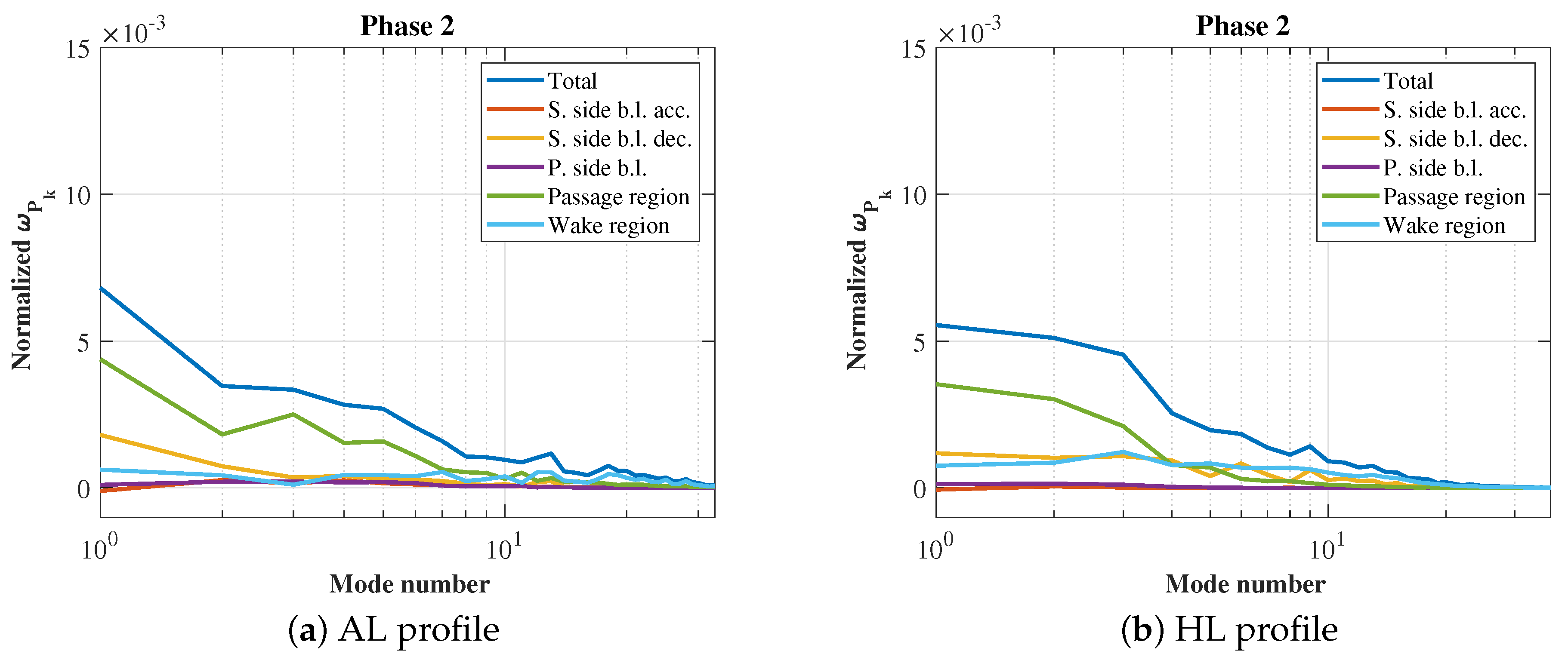
| (a) AL profile | (b) HL profile |
As noted earlier in this section, a new scenario emerges when the wake shifts towards the trailing edge, and the differences are clearly observed in the normalized plots reported in Figure 13. The analysis of PPOD mode 1 for the phase with the highest turbulent production (phase 7) allows us to pinpoint the position of the wake centerline, which, for both profiles, is located at the peak suction position. In this case, maximum turbulence production occurs on the rear suction side for both cascades, where the low-order modes associated with the upstream wake continue to dominate the loss generation mechanisms. During this phase, for the AL profile, significant losses are also generated within the wake region, and interestingly, higher-order modes contribute substantially to the generation process (see the cyan curve for mode indices greater than 9). The specific distribution of the blade loading characterizing the AL profile causes the point of maximum flow velocity around the blade to be located very close to the trailing edge, in contrast to what occurs with the HL profile.
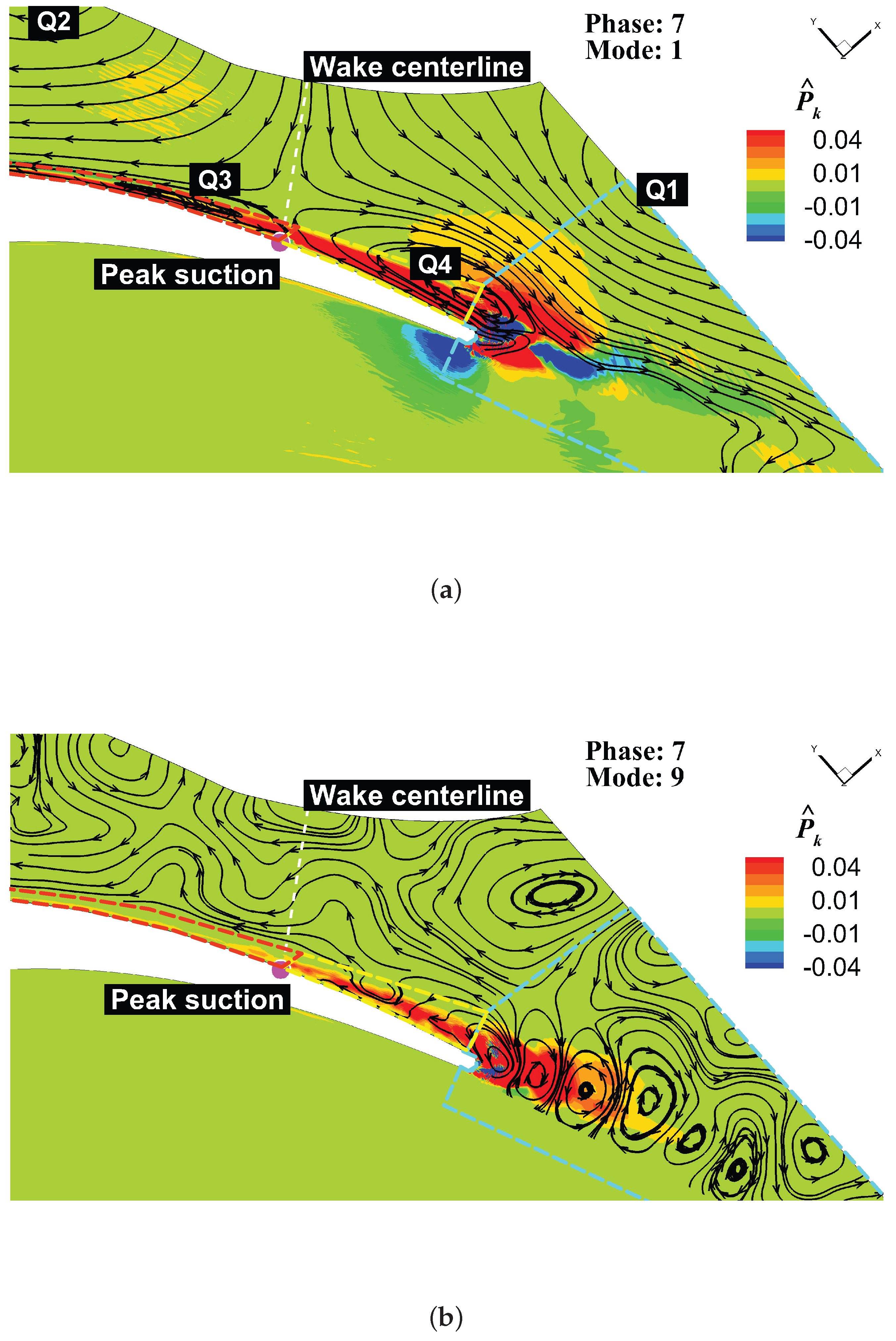
To better understand the different mechanisms involved in loss generation for both cascades, the contour plots in Figure 14 show the levels for PPOD mode 1 observed at phase 7, in a meridional section (located at midspan) of the rear part of the computational domain. This quantity represents a normalization of the production of TKE defined as:
The contour is overlaid with streamlines computed from the low-order reconstruction associated with each mode and centered around the peak suction position.
In addition to the previously identified Q1 and Q2 vortices, the figures highlight two other counter-rotating vortical structures, generated upstream and downstream of the wake centerline within the boundary layer. These are labeled as "Q3" and "Q4" vortices, and their formation is linked to the negative jet of the incoming wake. The modal representation of the flow obtained from the PPOD procedure enables the direct identification of the phase of maximum loss as the one characterized by the greatest amplification of these large-scale vortical structures.
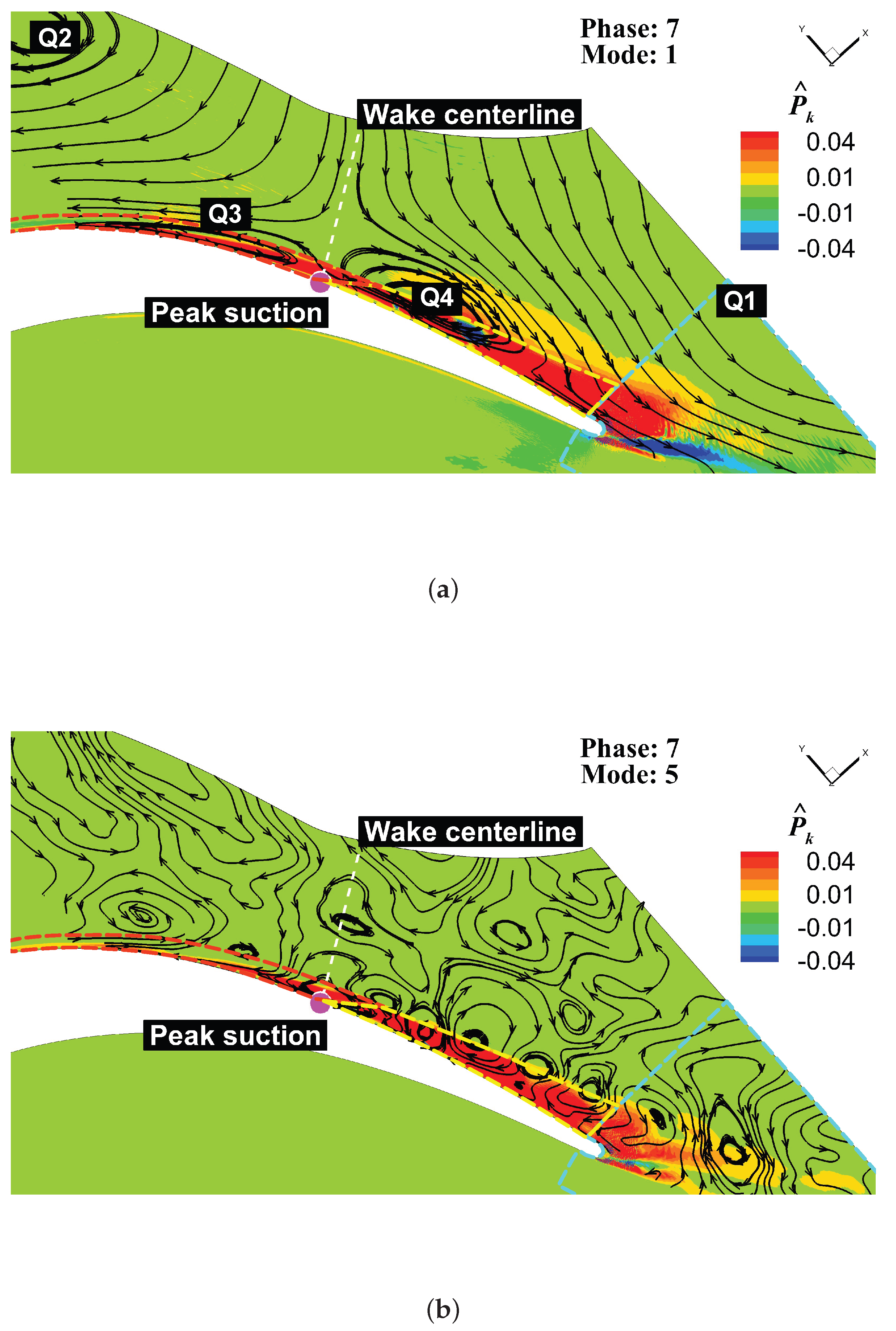
For what concerns the AL profile (Figure ), the proximity of the strongly amplified Q4 vortex to the trailing edge of the blade allows for the development of this structure further downstream in the wake region, as it is not spatially constrained by the presence of a solid wall. Observing the curve trends in Figure 13, a significant loss peak is noted in correspondence with mode 9 in the wake region (cyan curve). This mode captures the dynamics highlighted in Figure 15 by means of streamlines superimposed on the mode contour. It shows a clearly defined Von-Kármán vortex street, likely originating from the interaction between the Q4 vortex and the region of low momentum behind the trailing edge of the profile, which emerges as the main source of loss not directly related to the large-scale structures characterizing the upstream wake.
In the case of the HL profile, however, the upstream shift of the peak suction position causes the maximum spatial extent of the Q4 vortex to be limited, above by the Q1 vortex and below by the blade wall. Figure 15 shows that, under these conditions, the evolution of this vortex is largely confined within the boundary layer region. The highest loss peaks are indeed associated with the decelerating portion of the boundary layer (yellow curve in Figure 13). The most significant contribution to losses among the PPOD modes not related to the upstream wake is recorded in mode 5, whose two-dimensional representation is depicted in Figure 15. Mode 5 at phase 7 for the HL profile capture characteristic structures originating into the rear suction side. They are medium-scale roll-up vortices with axes aligned with the spanwise direction, which can be typically observed in the case of bypass-like transition mechanisms. The large-scale vortex structures observed for the AL profile within the wake region are not tracked by any of the HL profile’s modes at maximum loss phase.
Thus, the detailed analysis enabled by PPOD clearly allows the identification of maximum losses in the suction side BL region or within the wake downstream of the trailing edge when the upstream rotor wake is located at exactly the peak suction position. Depending on the blade loading, the structures captured by the higher-order PPOD modes interact with the boundary layer or the incoming wake, representing distinct contributions to the overall losses.
6. Conclusions
The application of Phase-locked Proper Orthogonal Decomposition (PPOD) to Large Eddy Simulations allows for a deep understanding of the loss generation mechanisms of low-pressure turbine blades operating with unsteady inflow conditions. The method enables for a detailed temporal and spatial analysis of the key drivers of profile losses, such as the upstream wake migration, boundary layer events, and vortex shedding phenomena.
The results emphasized the substantial impact of unsteady inflows and upstream wake interaction with boundary layers on the overall performance and efficiency of LPT blades. By separating and analyzing individual loss contributors in a phase-locked manner, we highlighted the differences in performance between the AL and HL profiles.
Losses observed in the passage region during phase 2 are primarily linked to the turbulence carried by the incoming wake, as the wake interaction with the boundary layer is marginal. Total loss in this phase is higher for the AL profile, with respect to the HL profile, and this is attributed to the mild acceleration imposed to the flow on the front part of the AL profile’s suction side.
When the wake approaches the peak suction position, losses within suction side boundary layer and wake region are notably affected. For the AL profile, flow dynamics associated with the evolution of the Q4 vortex result in significant turbulent production in the wake region, due to the formation of a Von Kármán vortex street downstream of the trailing edge.
Conversely, for the HL profile, the Q4 vortex is constrained by the Q1 vortex and the blade wall, limiting its spatial extent and confining most of the vortex evolution within the boundary layer. As a result, the primary losses are associated with the decelerating boundary layer rather than the wake region.
Overall, the observed differences in loss characteristics between the two profiles are largely due to variations in wake-related vortex dynamics and boundary layer behavior, influenced by the respective loading distributions and wake location at critical phases.
From an engineering perspective, the observed correlations between blade loading and the origin of large-scale vortex structures represent potential avenues for optimization of turbine blade design processes, focusing on minimizing loss-inducing events. Ultimately, this could lead to better predictive models for blade performance under varying operating conditions.
Acknowledgments
We acknowledge PRACE, which awarded access to the Fenix Infrastructure resources at CINECA, partially funded by the European Union’s Horizon 2020 research and innovation program through the ICEI project under the grant agreement No. 800858. We also acknowledge the CINECA award under the ISCRA initiative for the availability of high-performance computing resources and support.
Conflicts of Interest
The authors declare no conflicts of interest.
Nomenclature
The following nomenclature is used in this manuscript:
Roman symbols
| t | Time [s] |
| p | Pressure [Pa] |
| C | Chord [m] |
| Volume [m3] | |
| k | Turbulent kinetic energy [J kg−1] |
| V | Velocity [m s−1] |
| u | Velocity component [m s−1] |
| Mass flow rate [kg s−1] | |
| Re | Reynolds number, based on outlet velocity |
| Ma | Mach number |
| St | Strouhal number |
| AG | Dimensionless rotor-vane axial gap |
Greek symbols
| Kinematic viscosity [m2 s−1] | |
| Dynamic viscosity [Pa s] | |
| Density [kg m−3] | |
| Viscous stress tensor [Pa] | |
| Flow coefficient [-] |
Subscripts
| x | Axial component value |
| Axial chord-defined value | |
| t | Total/stagnation value |
| 1 | Inlet section value |
| 2 | Outlet section value |
| i | x-axis component value |
| j | y-axis component value |
Superscripts
| Time rate value | |
| Time-averaged value | |
| Time-fluctuating component value |
Abbreviations
The following abbreviations are used in this manuscript:
| CFD | Computational Fluid Dynamics |
| LES | Large Eddy Simulation |
| DNS | Direct Numerical Simulation |
| URANS | Unsteady Reynolds Averaged Navier-Stokes |
| WALE | Wall Adapting Local Eddy-viscosity |
| FV | Finite Volume |
| POD | Proper Orthogonal Decomposition |
| PPOD | Phase-locked Proper Orthogonal Decomposition |
| TKE | Turbulent Kinetic Energy |
| LPT | Low Pressure Turbine |
| FTT | Flow Through Time |
| BL | Boundary Layer |
| HPC | High-Performance Computing |
| ML | Machine Learning |
| PIV | Particle Image Velocimetry |
| F.A.S.P. | Flux of Average Stagnation Pressure |
| F.T.K.E. | Flux of Turbulent Kinetic Energy |
| V.D. | Viscous Diffusion |
| T.D. | Turbulent Diffusion |
| P.D. | Pressure Diffusion |
References
- Denton, J.D. Loss mechanisms in turbomachines. J. Turbomach. 1993, 115. [Google Scholar] [CrossRef]
- Rose, M.G.; Harvey, N.W. Turbomachinery wakes: Differential work and mixing losses. J. Turbomach. 2000, 122, 68–77. [Google Scholar] [CrossRef]
- Stieger, R.D.; Hodson, H.P. The unsteady development of a turbulent wake through a downstream low-pressure turbine blade passage. J. Turbomach. 2005, 127, 388–394. [Google Scholar] [CrossRef]
- Hodson, H.P.; Howell, R.J. Bladerow interactions, transition, and high-lift aerofoils in low-pressure turbines. Annu. Rev. Fluid Mech. 2005, 37, 71–98. [Google Scholar] [CrossRef]
- Sarkar, S.; Voke, P.R. Large-eddy simulation of unsteady surface pressure over a low-pressure turbine blade due to interactions of passing wakes and inflexional boundary layer. J. Turbomach. 2006, 128, 221–231. [Google Scholar] [CrossRef]
- Schulte, V.; Hodson, H.P. Unsteady wake-induced boundary layer transition in high lift LP turbines, 1998.
- Wu, X.; Jacobs, R.G.; Hunt, J.C.R.; Durbin, P.A. Simulation of boundary layer transition induced by periodically passing wakes. J. Fluid Mech. 1999, 398, 109–153. [Google Scholar] [CrossRef]
- Lengani, D.; Simoni, D.; Ubaldi, M.; Zunino, P.; Bertini, F. Coherent structures formation during wake-boundary layer interaction on a LP turbine blade. Flow Turbul. Combust. 2017, 98, 57–81. [Google Scholar]
- Sterzinger, P.Z.; Zerobin, S.; Merli, F.; Wiesinger, L.; Peters, A.; Maini, G.; Dellacasagrande, M.; Heitmeir, F.; Göttlich, E. Impact of varying high- and low-pressure turbine purge flows on a turbine center frame and low-pressure turbine system. J. Turbomach. 2020, 142, 101011. [Google Scholar] [CrossRef]
- Canepa, E.; Cattanei, A.F.; Mazzocut Zecchin, F.; Milanese, G.; Parodi, D. Experimental study of the effect of the rotor-stator gap variation on the tonal noise generated by low-speed axial fans. In Proceedings of the 19th AIAA/CEAS Aeroacoustics Conference, Berlin, Germany, 27–29 May 2013; p. 2046. [Google Scholar]
- Sandberg, R.D.; Michelassi, V. Fluid dynamics of axial turbomachinery: Blade- and stage-level simulations and models. Annu. Rev. Fluid Mech. 2022, 54, 255–285. [Google Scholar] [CrossRef]
- Lumley, J.L. The structure of inhomogeneous turbulent flows. In Atmospheric Turbulence and Radio Wave Propagation; Nauka: Moscow, 1967; pp. 166–178. [Google Scholar]
- Liu, Z.; Adrian, R.J.; Hanratty, T.J. Large-scale modes of turbulent channel flow: transport and structure. J. Fluid Mech. 2001, 448, 53–80. [Google Scholar] [CrossRef]
- van Oudheusden, B.W.; Scarano, F.; van Hinsberg, N.P.; Watt, D.W. Phase-resolved characterization of vortex shedding in the near wake of a square-section cylinder at incidence. Exp. Fluids 2005, 39, 86–98. [Google Scholar] [CrossRef]
- Perrin, R.; Cid, E.; Cazin, S.; Sevrain, A.; Braza, M.; Moradei, F.; Harran, G. Phase-averaged measurements of the turbulence properties in the near wake of a circular cylinder at high Reynolds number by 2C-PIV and 3C-PIV. Exp. Fluids 2007, 42, 93–109. [Google Scholar] [CrossRef]
- Kurelek, J.W.; Lambert, A.R.; Yarusevych, S. Coherent structures in the transition process of a laminar separation bubble. AIAA J. 2016, 54, 2295–2309. [Google Scholar] [CrossRef]
- Lengani, D.; Simoni, D.; Pichler, R.; Sandberg, R.D.; Michelassi, V.; Bertini, F. Identification and quantification of losses in a LPT cascade by POD applied to LES data. Int. J. Heat Fluid Flow 2018, 70, 28–40. [Google Scholar] [CrossRef]
- Dellacasagrande, M.; Lengani, D.; Simoni, D.; Ubaldi, M.; Granata, A.A.; Giovannini, M.; Rubechini, F.; Bertini, F. Analysis of Unsteady Loss Sensitivity to Incidence Angle Variation in Low Pressure Turbine. In Turbo Expo: Power for Land, Sea, and Air; American Society of Mechanical Engineers: 2023; Paper No. GT2023-103770.
- Canepa, E.; Lengani, D.; Nilberto, A.; Petronio, D.; Simoni, D.; Bertini, F.; Rosa Taddei, S. Flow coefficient and reduced frequency effects on low pressure turbine unsteady losses. J. Propuls. Power 2022, 38, 18–29. [Google Scholar] [CrossRef]
- Dellacasagrande, M.; Sterzinger, P.Z.; Zerobin, S.; Merli, F.; Wiesinger, L.; Peters, A.; Maini, G.; Heitmeir, F.; Göttlich, E. Unsteady Flow Interactions Between a High- and Low-Pressure Turbine: Part 2 — Rotor-Synchronic Averaging and Proper Orthogonal Decomposition of the Unsteady Flow Fields. In Turbo Expo: Power for Land, Sea, and Air; American Society of Mechanical Engineers: 2019; Volume 2A: Turbomachinery.
- Russo, M.; Carlucci, A.; Dellacasagrande, M.; Petronio, D.; Lengani, D.; Simoni, D.; Bellucci, J.; Giovannini, M.; Granata, A.A.; Gily, M.; Manca, C. Optimization of Low-Pressure Turbine Blade by Means of Fine Inspection of Loss Production Mechanisms. J. Turbomach. 2024, 147, 041005. [Google Scholar] [CrossRef]
- Nicoud, F.; Ducros, F. Subgrid-scale stress modelling based on the square of the velocity gradient tensor. Flow, Turbul. Combust. 1999, 62, 183–200. [Google Scholar] [CrossRef]
- Benhamadouche, S.; Jarrin, N.; Addad, Y.; Laurence, D. Synthetic turbulent inflow conditions based on a vortex method for large-eddy simulation. Prog. Comput. Fluid Dyn. 2006, 6, 50–57. [Google Scholar] [CrossRef]
- Przytarski, P.; Lengani, D.; Simoni, D.; Wheeler, A.P.S. The Role of Turbulence Transport in Mechanical Energy Budgets. J. Turbomach. 2024. [Google Scholar] [CrossRef]
- Sirovich, L. Turbulence and the dynamics of coherent structures, Parts I, II and III. Quart. Appl. Math. 1987, 561–590. [Google Scholar] [CrossRef]
- Biassoni, D.; Russo, M.; Viviani, P.; Vitali, G.; Lengani, D. A High-Performance Code for Analyzing Loss Transport Equations in High-Fidelity Simulations. In Turbo Expo: Power for Land, Sea, and Air; American Society of Mechanical Engineers: 2024; paper No. GT2024-127953.
- Leggett, J.; Priebe, S.; Shabbir, A.; Michelassi, V.; Sandberg, R.; Richardson, E. Loss prediction in an axial compressor cascade at off-design incidences with free stream disturbances using large eddy simulation. J. Turbomach. 140, 7 (2018).
- Michelassi, V.; Chen, L.; Pichler, R.; Sandberg, R.; Bhaskaran, R. High-fidelity simulations of low-pressure turbines: Effect of flow coefficient and reduced frequency on losses. Journal of Turbomachinery 138, 11 (2016).
- Perrin, R.; Braza, M.; Cid, E.; Cazin, S.; Barthet, A.; Sevrain, A.; Mockett, C.; Thiele, F. Obtaining phase averaged turbulence properties in the near wake of a circular cylinder at high Reynolds number using POD. Experiments in Fluids 43, 341–355 (2007).
- Lengani, D.; Simoni, D.; Nilberto, A.; Ubaldi, M.; Zunino, P.; Bertini, F. Synchronization of multi-plane measurement data by means of POD: application to unsteady boundary layer transition. Experiments in Fluids 59, 1–18 (2018).
- Simoni, D.; Berrino, M.; Ubaldi, M.; Zunino, P.; Bertini, F. Off-design performance of a highly loaded low pressure turbine cascade under steady and unsteady incoming flow conditions. Journal of Turbomachinery 137, 7 (2015). American Society of Mechanical Engineers, paper No. TURBO-14-1280.
- Berrino, M.; Lengani, D.; Simoni, D.; Ubaldi, M.; Zunino, P.; Bertini, F. Dynamics and turbulence characteristics of wake-boundary layer interaction in a low pressure turbine blade. In Turbo Expo: Power for Land, Sea, and Air (2015). American Society of Mechanical Engineers, paper No. GT2015-42626.
- Stieger, R.D.; Hodson, H.P. The transition mechanism of highly loaded low-pressure turbine blades. J. Turbomach. 126, 4 (2004), 536–543.
- Lengani, D.; Simoni, D.; Ubaldi, M.; Zunino, P.; Bertini, F.; Michelassi, V. Accurate Estimation of Profile Losses and Analysis of Loss Generation Mechanisms in a Turbine Cascade. Journal of Turbomachinery 139, 12 (2017), 121007.
- Hekmati, A.; Ricot, D.; Druault, P. About the convergence of POD and EPOD modes computed from CFD simulation. Computers & Fluids 50, 1 (2011), 60-71. [CrossRef]
- Pope, S.B. Ten questions concerning the large-eddy simulation of turbulent flows. New Journal of Physics 6, 1 (2004), 35.
Figure 1.
Schematic of the stage-like simulation environment for unsteady inflow conditions
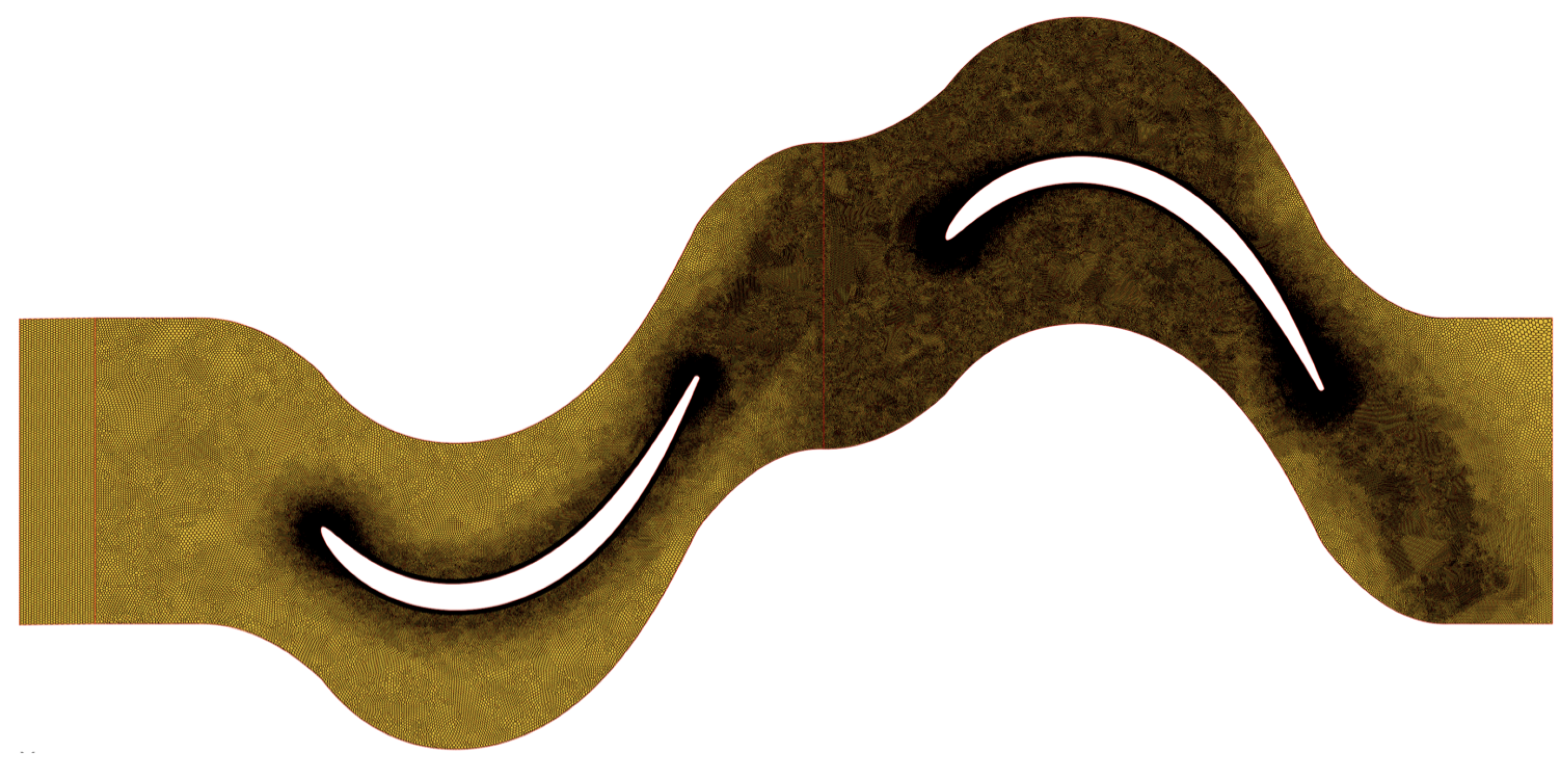
Figure 2.
Distribution of Pope’s criterion M and normalized turbulent kinetic energy across the vane computational domain.
Figure 2.
Distribution of Pope’s criterion M and normalized turbulent kinetic energy across the vane computational domain.
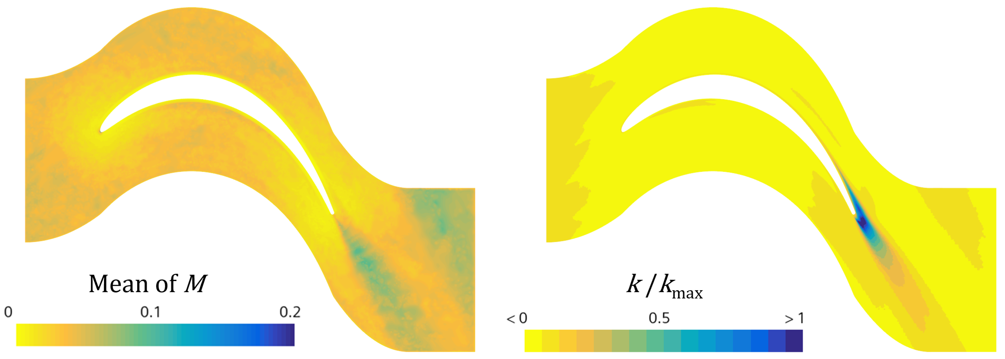
Figure 3.
Isosurfaces of POD mode 1 for the two profiles. They are representative of the evolution of the incoming wake from LE to TE
Figure 3.
Isosurfaces of POD mode 1 for the two profiles. They are representative of the evolution of the incoming wake from LE to TE
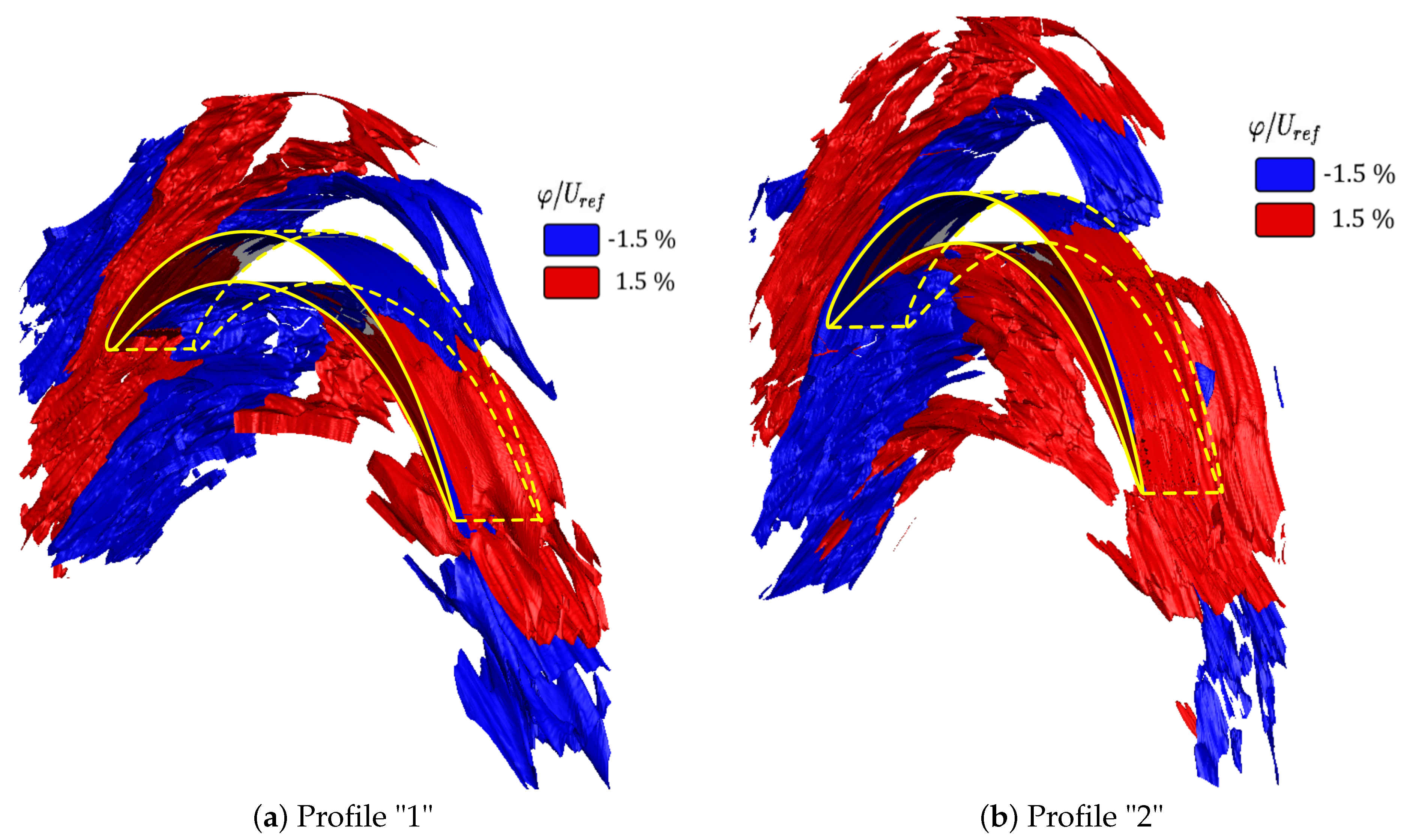
| (a) Profile "1" | (b) Profile "2" |
Figure 4.
Simplified diagram representative of the snapshot sorting procedure, based on the phase shift between the first two POD eigenvectors
Figure 4.
Simplified diagram representative of the snapshot sorting procedure, based on the phase shift between the first two POD eigenvectors
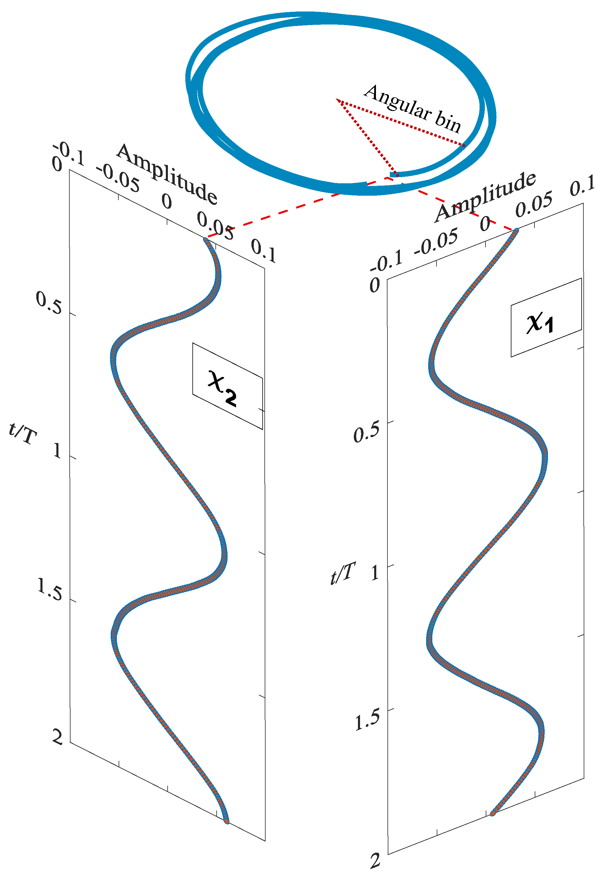
Figure 5.
Sub-regions for integration of viscous and turbulent losses
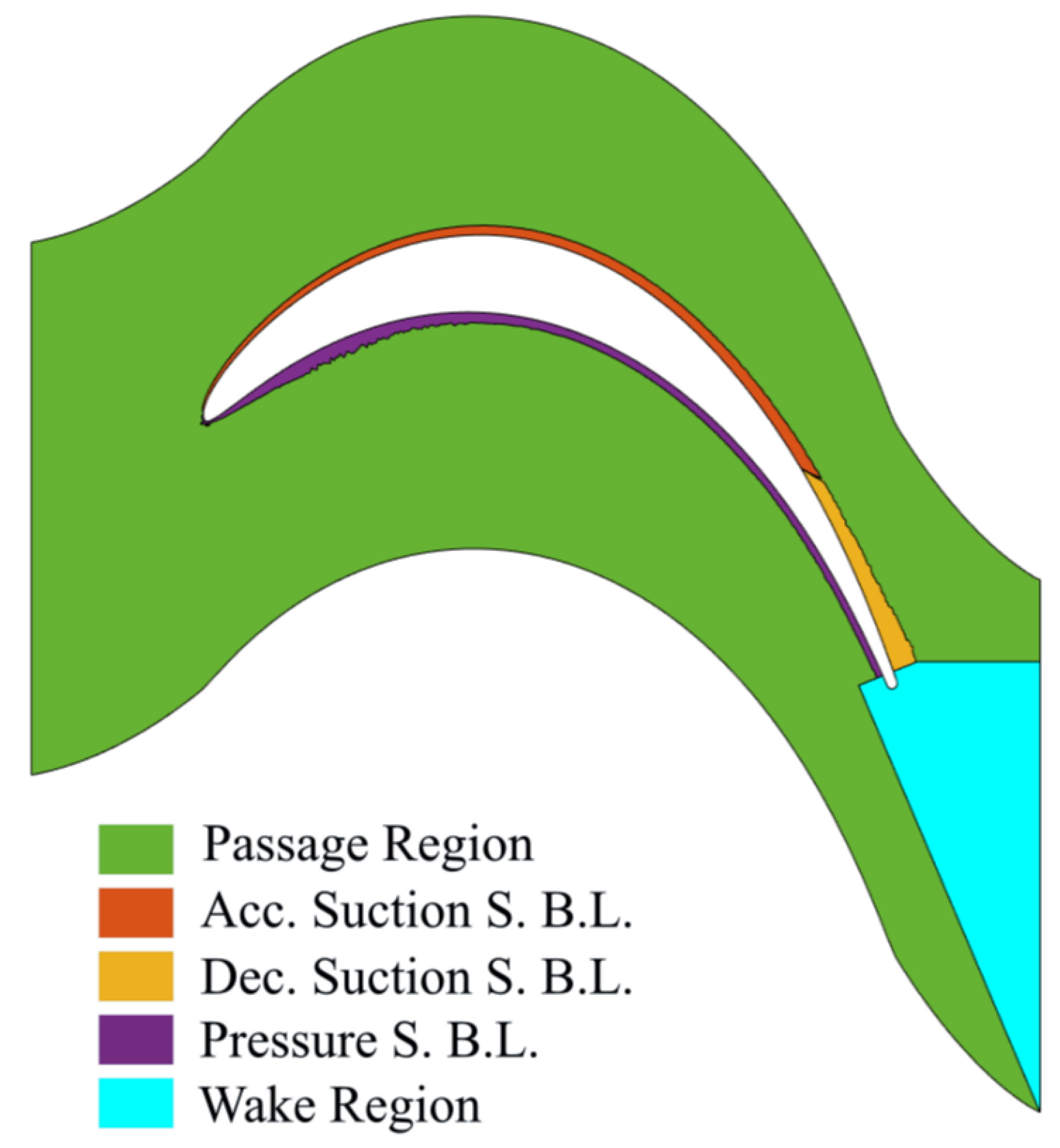
Figure 6.
Distribution of normalized for the two blade profiles
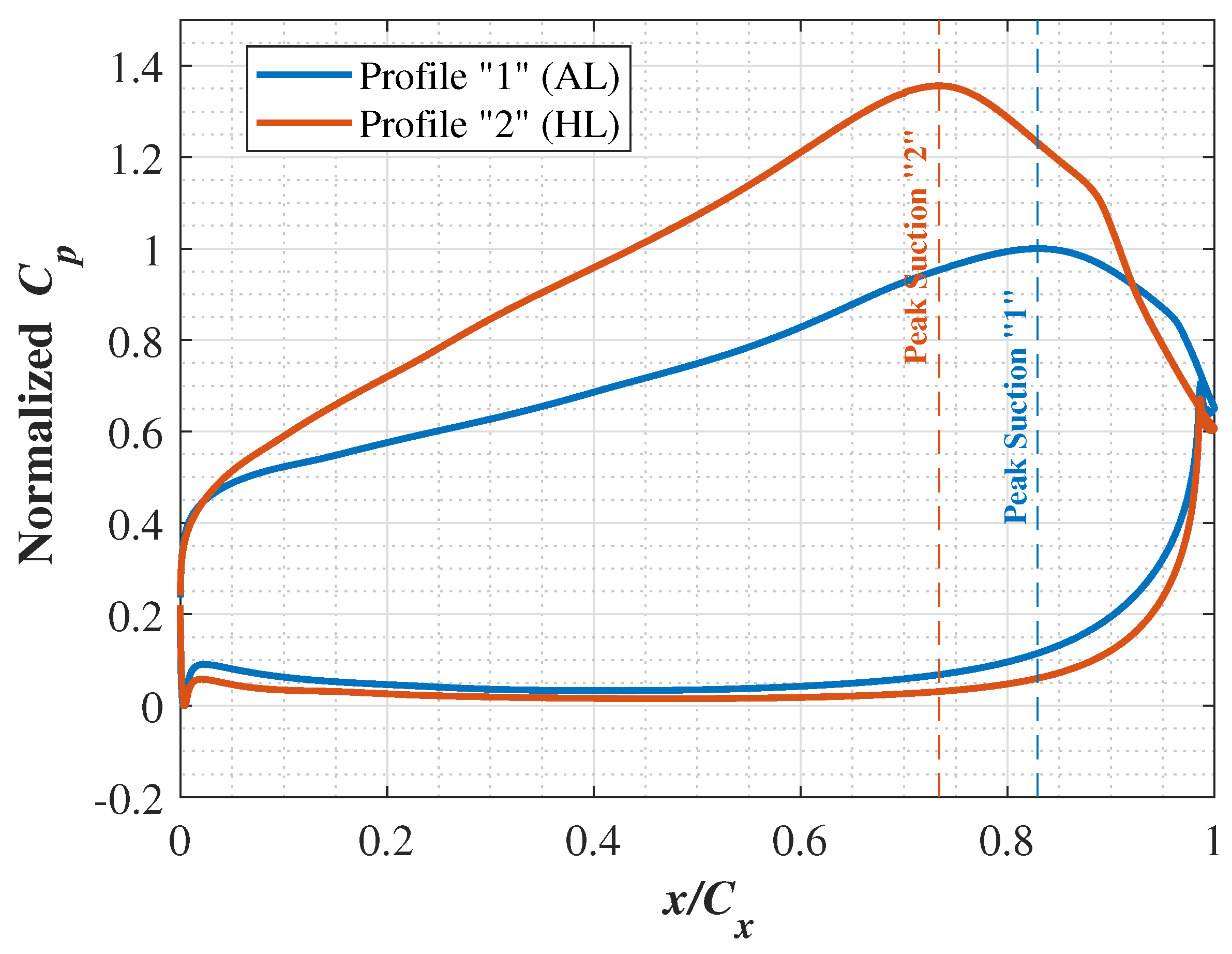
Figure 7.
POD mode cumulative contribution to stagnation pressure losses for the AL profile
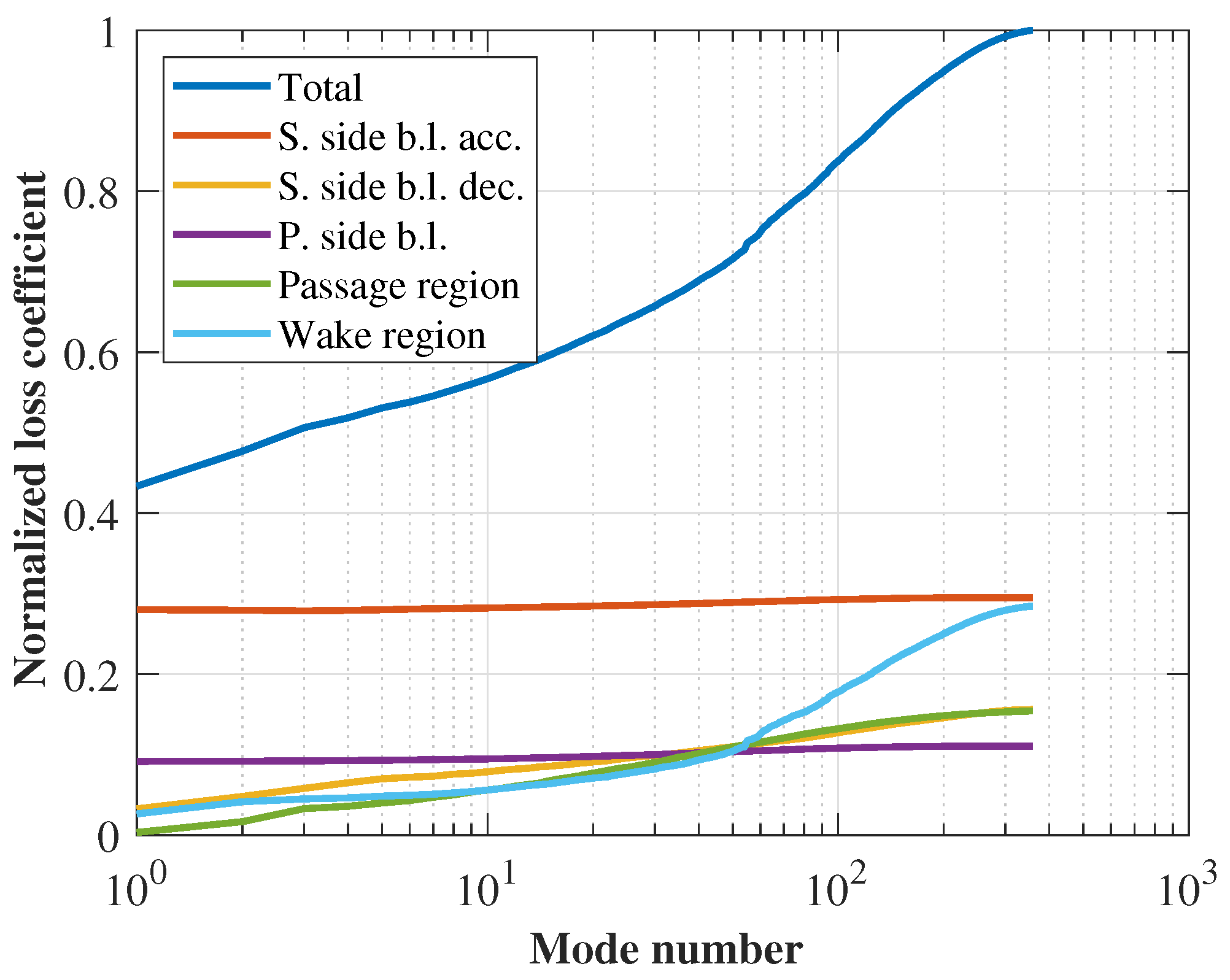
Figure 8.
POD mode cumulative contribution to stagnation pressure losses for the HL profile
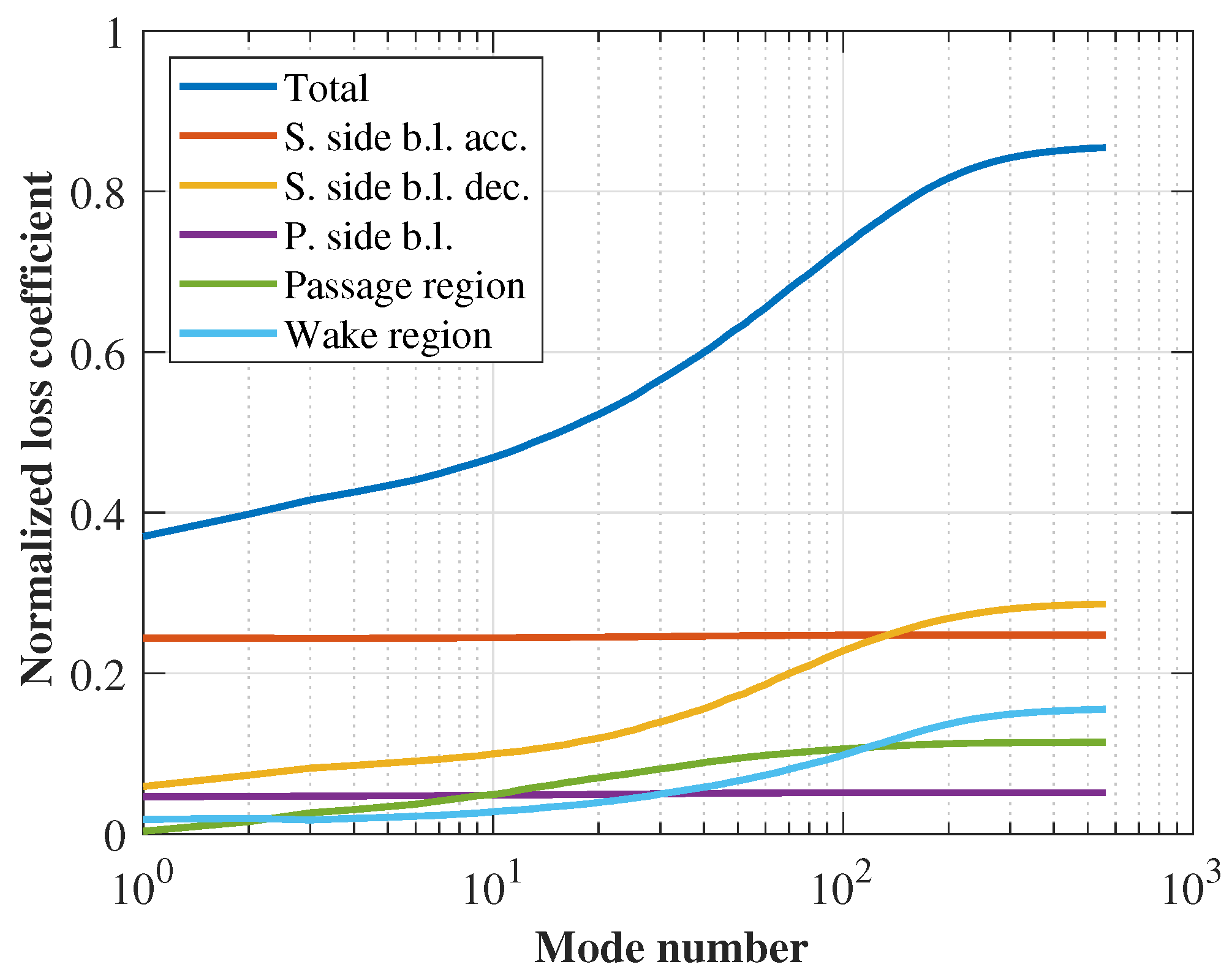
Figure 9.
Contour plots of HL profile’s PPOD mode 1 of the stream-parallel velocity component for phases 2 and 7, normalized with a reference velocity and overlaid to mode streamlines
Figure 9.
Contour plots of HL profile’s PPOD mode 1 of the stream-parallel velocity component for phases 2 and 7, normalized with a reference velocity and overlaid to mode streamlines
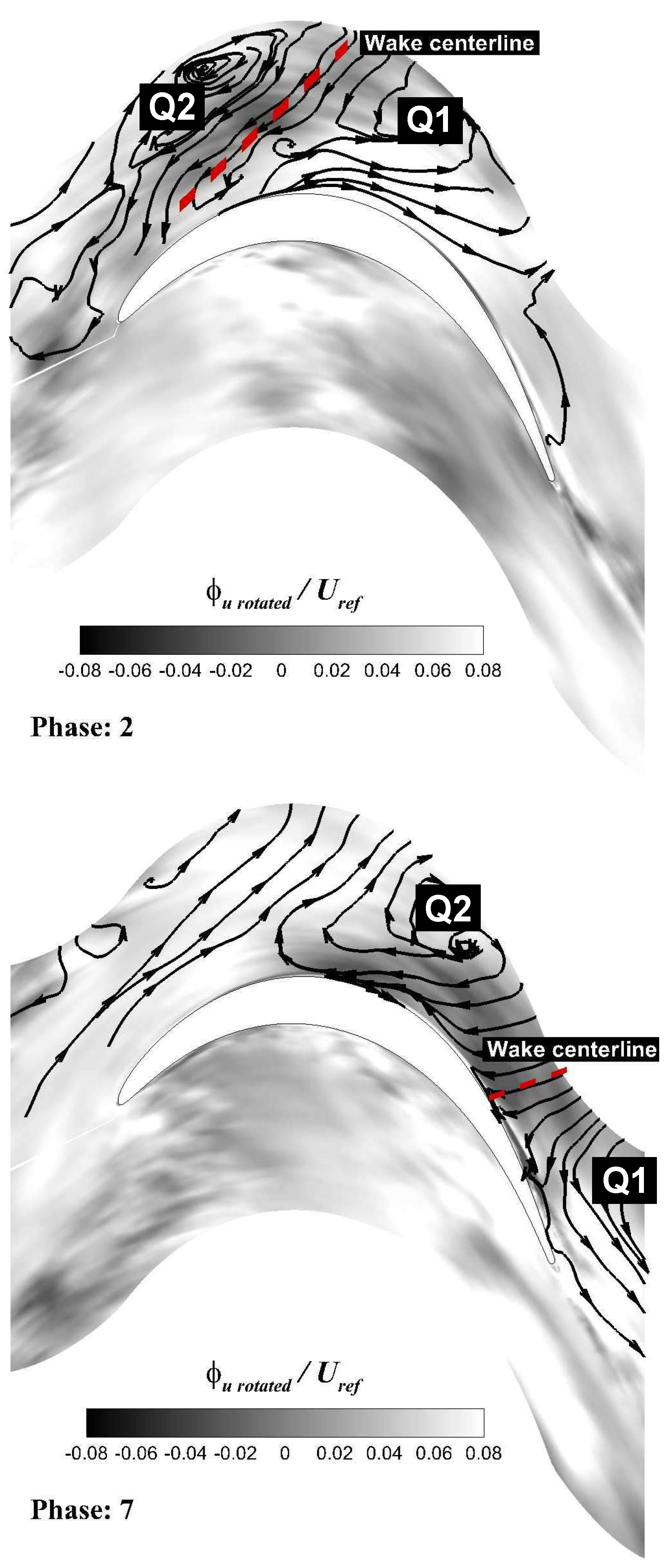
Figure 10.
Bar charts of normalized loss coefficient (computed from -only contribution) for each of the 10 wake passing phases for the AL profile
Figure 10.
Bar charts of normalized loss coefficient (computed from -only contribution) for each of the 10 wake passing phases for the AL profile
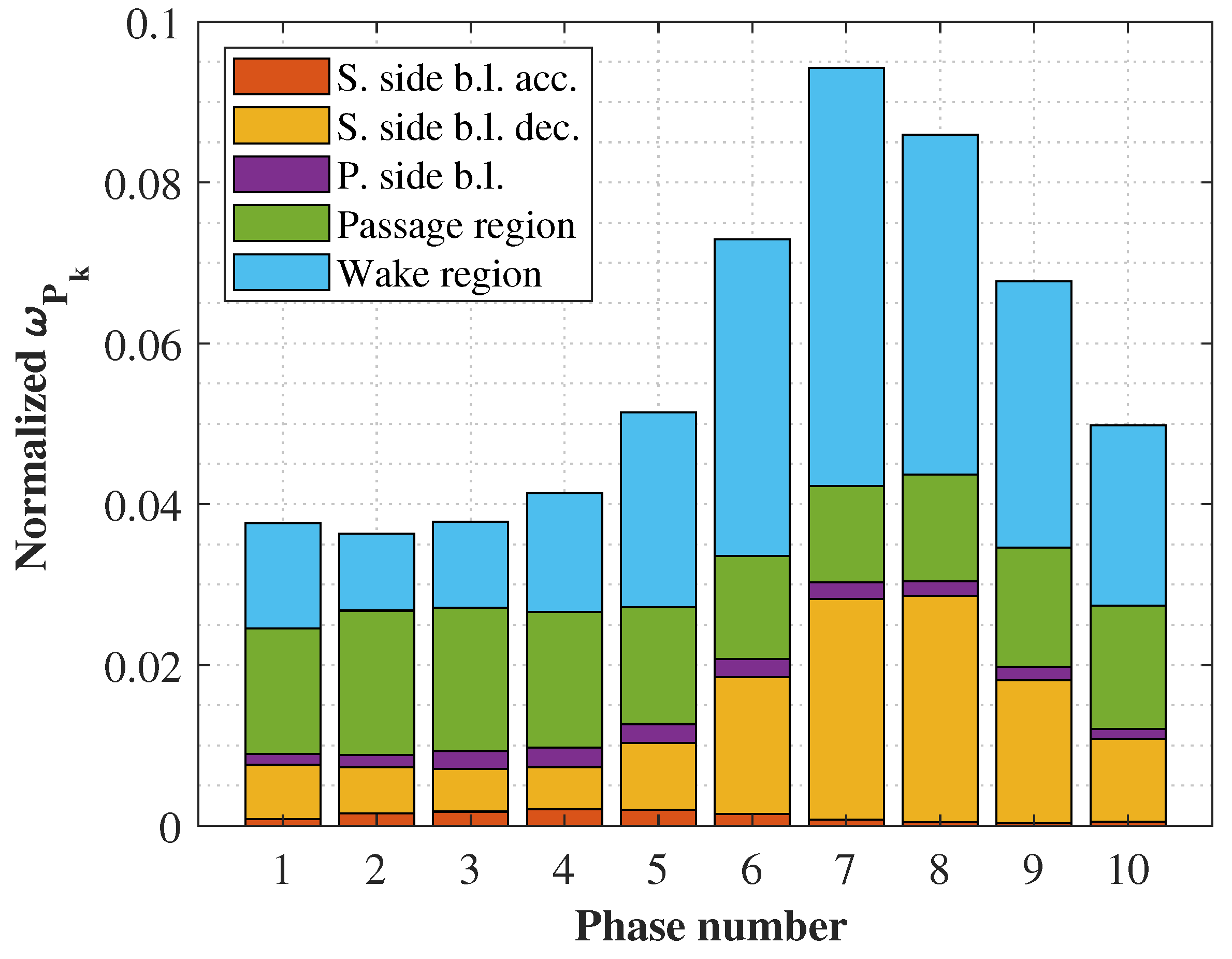
Figure 11.
Bar charts of normalized loss coefficient (computed from -only contribution) for each of the 10 wake passing phases for the HL profile
Figure 11.
Bar charts of normalized loss coefficient (computed from -only contribution) for each of the 10 wake passing phases for the HL profile
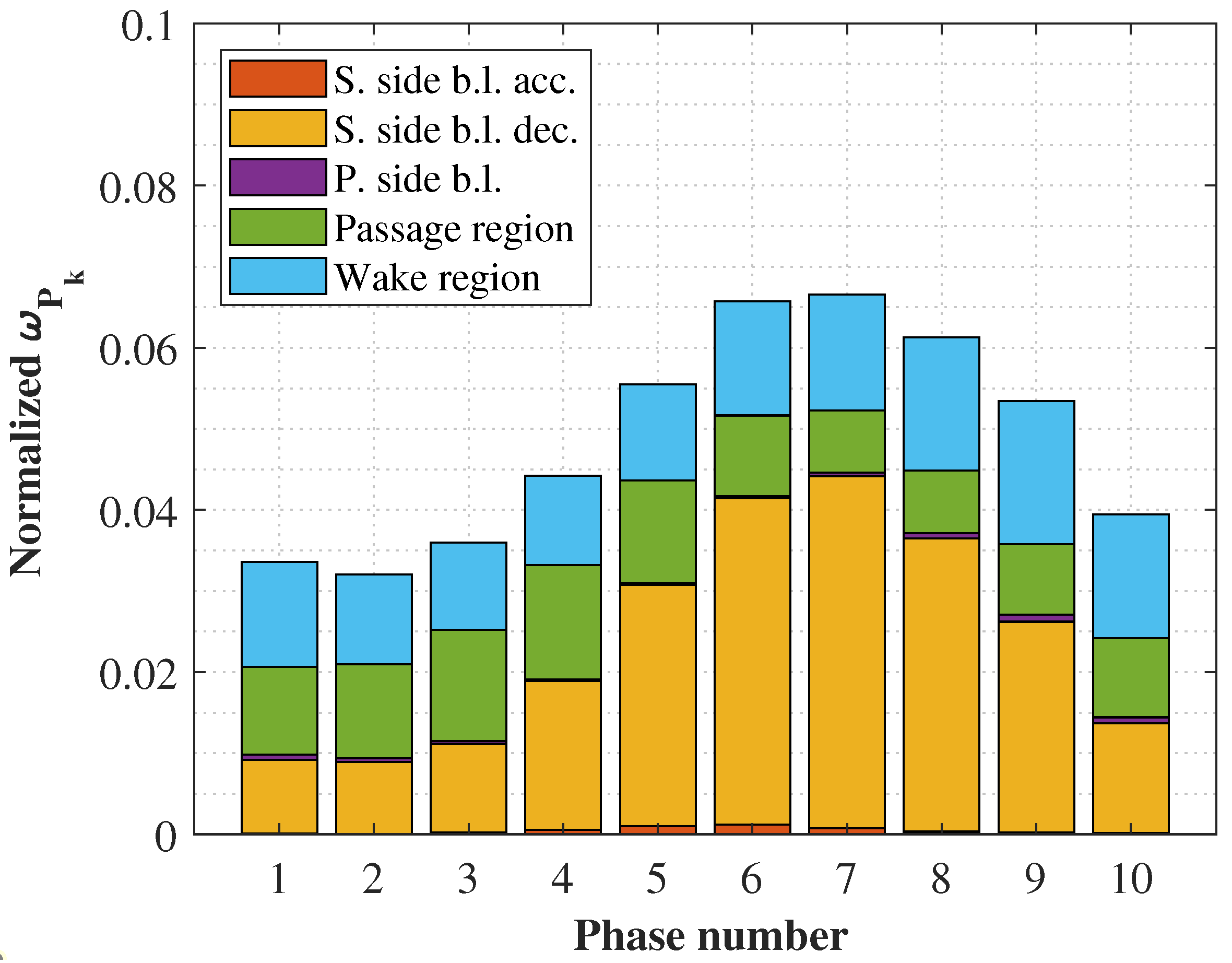
Figure 13.
Plots of normalized as a function of phase 7 mode index for (a) the Aft-Loaded and (b) the High-Loaded cascades. Blue curve represent the total mode contribution from the five sub-regions
Figure 13.
Plots of normalized as a function of phase 7 mode index for (a) the Aft-Loaded and (b) the High-Loaded cascades. Blue curve represent the total mode contribution from the five sub-regions
| (a) AL profile | (b) HL profile |
Figure 14.
Contour plots of AL profile’s mode 1 (panel a on the left) and 9 (panel b on the right) of the dimensionless TKE production at phase 7, overlaid to the corresponding mode streamlines. The extent of the integration sub-regions is marked by dashed lines adopting the color scheme as in Figure 5.
| (a) | |
| (b) |
Figure 15.
Contour plots of HL profile’s mode 1 (panel a on the left) and 5 (panel b on the right) of the dimensionless TKE production at phase 7, overlaid to the corresponding mode streamlines. The extent of the integration sub-regions is marked by dashed lines adopting the color scheme as in fig. Figure 5.
| (a) | |
| (b) |

Table 1.
LES calculation conditions
| Profile | "1" | "2" |
|---|---|---|
| 1.11 | 1.11 | |
| St | 1.08 | 0.73 |
| AG | 0.65 | 0.65 |
Table 2.
Normalized experimental and numerical loss coefficients
| Profile | "1" | "2" |
|---|---|---|
| Exp. loss coeff. | 1.00 | 0.79 |
| LES loss coeff. | 0.95 | 0.75 |
| LES-to-exp. ratio | 0.95 | 0.95 |
Disclaimer/Publisher’s Note: The statements, opinions and data contained in all publications are solely those of the individual author(s) and contributor(s) and not of MDPI and/or the editor(s). MDPI and/or the editor(s) disclaim responsibility for any injury to people or property resulting from any ideas, methods, instructions or products referred to in the content. |
© 2025 by the authors. Licensee MDPI, Basel, Switzerland. This article is an open access article distributed under the terms and conditions of the Creative Commons Attribution (CC BY) license (http://creativecommons.org/licenses/by/4.0/).
Copyright: This open access article is published under a Creative Commons CC BY 4.0 license, which permit the free download, distribution, and reuse, provided that the author and preprint are cited in any reuse.


