Reassessing the Discounted Cash Flow Model (DCFM): How the Potential Payback Period (PPP) Improves Applicability and Accuracy with a Time-Based Approach

1. Introduction: From Discounted Flows to Timed Returns

Valuation underpins modern finance—guiding decisions in investment management, corporate strategy, and equity research. Among the many models developed to estimate intrinsic value, the Discounted Cash Flow Model (DCFM) holds historical dominance. By valuing an asset as the present value of future cash flows, discounted for time and risk, the DCFM has long been a theoretical benchmark.

Yet in practice, the DCFM often falters. The more distant the forecast, the greater the uncertainty. Terminal values—intended to simplify the indefinite future—often dominate total valuation, distorting the analysis. These flaws have become more pronounced in today’s environment, where fast-changing markets and unpredictable earnings challenge conventional modeling.

This paper introduces the Potential Payback Period (PPP) as a modern alternative: a valuation model that retains the DCFM’s theoretical core but replaces speculation with structure. By framing valuation around how long it takes for cumulative earnings to recover the price paid, the PPP offers a pragmatic and rate-based answer to the timeless valuation question.

2. Origins and Limitations of the Discounted Cash Flow Model (DCFM)

The traditional DCFM calculates the present value of a stream of future free cash flows using the following formula:

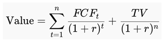
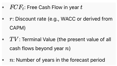
Where:

2.1. Historical Foundations

The DCF approach dates to John Burr Williams’s 1938 classic The Theory of Investment Value, where he argued that a stock’s worth equals the present value of expected future dividends. This evolved into the free cash flow-based DCFM used today in corporate finance, further refined by the Capital Asset Pricing Model (CAPM) and modern risk-adjusted discounting.

As academic theory turned into industry practice, the DCFM became the dominant framework taught in MBA programs and applied in investment banking, valuation, and corporate finance.

2.2. Structural Weaknesses

Despite its pedigree, the DCFM suffers from four key limitations:

• Speculative Forecasting: Long-range FCF projections are inherently fragile and assumption-laden.
• Terminal Value Distortion: Terminal values often comprise 60–80% of the model’s output, based on arbitrary perpetual growth assumptions.
• Opacity and Subjectivity: Numerous assumptions reduce transparency and make results difficult to audit or reproduce.
• No Rate-of-Return Output: Unlike bonds that yield an annualized return (YTM), DCFM provides a price, not a rate—limiting cross-asset comparison.

These weaknesses call for a methodology that simplifies forecasting, clarifies assumptions, and outputs rate-based returns. The PPP answers that call.

3. Introducing the Potential Payback Period (PPP)

The Potential Payback Period (PPP) reorients valuation around a fundamental and intuitive question:

How long does it take for a stock’s cumulative earnings—adjusted for growth and discounted for risk—to pay back its purchase price?

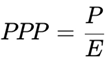
3.1. Core Formula

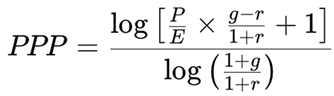
Where:

• P/E: Price-to-Earnings ratio
• g: Expected annual earnings growth rate
• r: Discount rate (e.g., from CAPM)

This formula remains valid under extreme conditions:

• When g = r, it simplifies to:

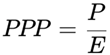
• When g = 0 and r = 0, it again reduces to:

This confirms that PPP generalizes the P/E ratio while maintaining mathematical robustness.

3.2. Doubling Formula for SIRR

Once the PPP is determined, the Stock Internal Rate of Return (SIRR)—based solely on cumulative earnings—is given by the Doubling Formula:

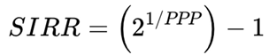
This version emphasizes the central role of 2, reflecting the goal of doubling the initial investment over the Potential Payback Period (PPP) using earnings alone.

This formulation is mathematically equivalent to:

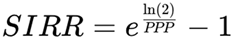
But it offers a more intuitive interpretation: it represents the annualized rate of return that, if applied to the original investment and compounded over PPP years, would result in exactly twice the initial amount. In other words, SIRR answers the question: What annual return is required to recover the original investment purely through cumulative earnings over the PPP timeframe, assuming reinvestment but excluding dividends and price appreciation?

4. Adding Price Appreciation: From SIRR to SIRRIPA

While the SIRR focuses solely on cumulative earnings, most investors also benefit from eventual price appreciation. The PPP framework integrates this consideration through a second metric: SIRR Including Price Appreciation (SIRRIPA).

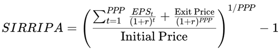
This formula accounts for both the discounted value of interim earnings and the final Exit Price.

4.1. Why Exit P/E = PPP

In the PPP framework, the Exit P/E is not arbitrarily chosen—it is logically defined as:>

Exit P/E = PPP

This relationship emerges from the internal logic of the model: if a stock earns back its price through discounted earnings over PPP years, and if the earnings growth and discount rates converge (i.e., g = r), then the appropriate terminal valuation multiple becomes equal to the PPP itself.

Accordingly, the Exit Price is calculated as:

Exit Price = EPS_end X PPP

This ensures internal consistency between the initial valuation, the assumed earnings trajectory, and the terminal valuation.

5. Comparative Analysis: DCFM vs. PPP in Practice

5.1. Example Scenario

Let us consider the following input assumptions for a hypothetical stock:

• Price = $100
• EPS = $5 → P/E = 20
• g = 10% expected earnings growth
• r = 8% discount rate

DCFM:

In standard practice, the DCFM projects 10 years of Free Cash Flows (FCFs), followed by a terminal value based on a 3% perpetual growth rate. This structure reflects a conventional compromise:

• Ten-year forecast horizon: While future earnings or cash flows could theoretically extend indefinitely, projecting more than 10 years becomes increasingly speculative. A 10-year horizon is widely accepted as the outer boundary for “plausible” forecasts in most industries, balancing model complexity with diminishing confidence in long-term estimates.
• Terminal growth rate of 3%: This figure is typically used to approximate the long-run growth of the overall economy (e.g., GDP growth or inflation-adjusted output). The assumption is that after 10 years, the company matures and grows at a modest, sustainable pace indefinitely.

However, this DCF structure creates significant sensitivity to assumptions:

• Most of the stock’s estimated intrinsic value (often 60–80%) comes from the terminal value—which is itself based on highly uncertain assumptions about steady-state growth and cash flow behavior a decade into the future.
• Small changes to the 3% terminal growth or the 10th-year FCF can drastically alter the valuation, reducing reliability and transparency.

PPP Approach:

By contrast, the PPP model avoids the need to assume a terminal value or forecast cash flows beyond what is operationally recoverable. Using the same inputs:

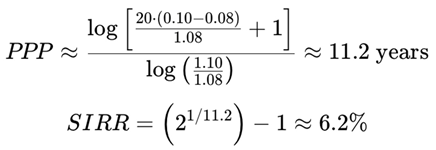
This result—an annualized return based solely on earnings recovery—can be directly benchmarked against a 10-year Treasury yield of, say, 4.5%, offering rate-based clarity absent from the DCFM’s output price.

6. When DCF Fails and PPP Persists

The PPP remains usable even where DCFM collapses:

• Negative or erratic FCFs: PPP operates on normalized EPS.
• g ≈ r: No instability—the formula remains defined.
• No dividends or unclear terminal value: PPP requires neither.
• Loss-making firms: With expected normalized earnings, PPP can still yield a meaningful time horizon.

For high-growth, high-risk companies with volatile cash flows and uncertain exits, PPP offers a conservative yet consistent valuation benchmark.

7. Conclusion: From Cash Flow Speculation to Time-Based Precision

The Potential Payback Period (PPP) reframes equity valuation from speculative forecasting to operational recovery. Rooted in observable metrics, it restores clarity and comparability to financial analysis.

Unlike the DCFM, which yields a speculative price, the PPP yields a return-based horizon—enabling investors to ask: Is this stock worth it, given how long it will take to pay itself back, with or without price appreciation?

By transforming valuation into a transparent, rate-based process, the PPP bridges the gap between theory and practice—and brings financial modeling into alignment with modern investment needs.

References

- Williams, J. B. The Theory of Investment Value; Harvard University Press, 1938. [Google Scholar]
- Sharpe, W. F. Capital Asset Prices: A Theory of Market Equilibrium under Conditions of Risk. The Journal of Finance 1964, 19(3), 425–442. [Google Scholar] [CrossRef]
- Damodaran, A. Investment Valuation: Tools and Techniques for Determining the Value of Any Asset, 3rd ed.; Wiley Finance, 2012. [Google Scholar] [CrossRef]
- Penman, S. H. Financial Statement Analysis and Security Valuation, 5th ed.; McGraw-Hill Education, 2013. [Google Scholar]
- Fernández, P. Company Valuation Methods; IESE Business School, 2015; Available online: https://ssrn.com/abstract=2749731.
- Luehrman, T. A. Using APV: A Better Tool for Valuing Operations. Harvard Business Review May-June 1997. https://hbr.org/1997/05/using-apv-a-better-tool-for-valuing-operations. [Google Scholar]
- Sam, R. Extending the P/E and PEG Ratios: The Role of the Potential Payback Period (PPP) in Modern Equity Valuation. SSRN 2024. Available online: https://ssrn.com/abstract=5240458.
- Sam, R. Revisiting the Gordon-Shapiro Model: How the Potential Payback Period (PPP) Refines and Operationalizes a Foundational Framework in Stock Valuation. SSRN 2025. Available online: https://ssrn.com/abstract=5248835.
- Sam, R. Breaking the Valuation Deadlock: Replacing the P/E Ratio with the Potential Payback Period (PPP) for Loss-Making Companies – A Case Study on Intel (2025). SSRN 2025. [Google Scholar]
- Sam, R. Generalizing the P/E Ratio through the Potential Payback Period (PPP): A Dynamic Approach to Stock Valuation. SSRN 2025. Available online: https://ssrn.com/abstract=5261816.
- Sam, R. Proving that the P/E Ratio is Just a Limiting Case of the Potential Payback Period (PPP) When Earnings Growth and Interest Rate are Ignored. SSRN 2025. Available online: https://ssrn.com/abstract=5254723.
- Sam, R. How the Potential Payback Period (PPP) Extends and Surpasses the Gordon Growth Model (GGM) at the Limits of Financial Theory. In SSRN; /: https, 2025. [Google Scholar]
- Sam, R. A Quantitative Revelation in Equity Valuation: The P/E Ratio is a Degenerate Case of the Potential Payback Period (PPP). In SSRN; 2025; Available online: https://ssrn.com/abstract=5268285.
- Brealey, R.A.; Myers, S.C.; Allen, F. Principles of Corporate Finance, 13th ed.; McGraw-Hill Education, 2020. [Google Scholar]
Disclaimer/Publisher’s Note: The statements, opinions and data contained in all publications are solely those of the individual author(s) and contributor(s) and not of MDPI and/or the editor(s). MDPI and/or the editor(s) disclaim responsibility for any injury to people or property resulting from any ideas, methods, instructions or products referred to in the content. |
© 2025 by the author. Licensee MDPI, Basel, Switzerland. This article is an open access article distributed under the terms and conditions of the Creative Commons Attribution (CC BY) license (https://creativecommons.org/licenses/by/4.0/).
Copyright: This open access article is published under a Creative Commons CC BY 4.0 license, which permit the free download, distribution, and reuse, provided that the author and preprint are cited in any reuse.