Submitted:
03 June 2025
Posted:
03 June 2025
You are already at the latest version
Abstract
In order to evaluate the classification performance of an algorithm, it is necessary to partition the original dataset into training and test subsets. After constructing a classification model using the training dataset, the test dataset is utilized to evaluate its accuracy. However, accurately assessing classification performance typically requires multiple rounds of training/test data sampling, model construction, and accuracy evaluation, followed by averaging the results. This process is computationally expensive and time-consuming. To address this issue, we propose an effective sampling approach that allows for the selection of training and test sets which closely approximate the outcomes derived from repeated sampling and evaluation processes. Our approach ensures that the sampled data closely reflects the classification performance on the original dataset. Specifically, we introduce various techniques to measure the similarity of data distributions and incorporate feature weighting in the similarity computation, allowing us to select training and test sets that best preserve the distributional characteristics of the original dataset.
Keywords:
data sampling
; classification
; accuracy evaluation
; data distribution
1. Introduction
In the process of constructing a classification model, the data sampling method plays a crucial role. The model's learning capability is highly dependent on the quality of the sampled training set, while its accuracy is determined by the test set. If the sampling method results in a poor-quality training set for model construction and an overly simple test set, the model may achieve artificially high accuracy, leading to a misjudgment of its actual performance.
Therefore, during the data sampling phase, it is essential to carefully select samples to ensure their representativeness. This requires adopting appropriate sampling strategies and ensuring diversity within the sample to accurately reflect the overall data distribution. One of the most commonly used sampling methods is random sampling, which is both simple and efficient. In this approach, each data point has an equal probability of being selected, making the sampled dataset a reasonable representation of the entire population. Due to its ease of implementation, random sampling is frequently used in practical applications.
Random sampling has the drawback of generating different training and test sets in each iteration, leading to variations in accuracy results. A single instance of random sampling cannot fully reflect the model's performance, making it unreliable for evaluating classification models when only one training/test split is used. To achieve a more accurate assessment, multiple random samplings are typically required, and the average accuracy across all experiments is used as a measure of overall performance. However, this approach necessitates training multiple models, which is computationally expensive and impractical for real-world applications. Cross-validation offers a solution by mitigating the limitations of single random sampling. By systematically rotating different subsets of data into the training and test sets and averaging the results, cross-validation provides a more comprehensive evaluation of model performance. Given these limitations of random sampling, improving sampling strategies and efficiently selecting appropriate training and test sets have become crucial research topics in the field [7,8,9,10].
The random sampling method presents several challenges in constructing classification models, particularly in terms of efficiency, time consumption, and computing resource demands for model evaluation. These factors significantly impact its practicality in real-world applications. To address these issues, Shin and Oh [6] proposed an improved sampling method FWS based on the approach introduced by Kang and Ohs [4]. Their method involves performing multiple random samplings to generate multiple training/test datasets as candidates. For each set, feature-weighted distance between this set and original dataset is calculated to assess their suitability. A training/test set is then selected from these multiple candidates to optimize model performance. However, this method still faces difficulties in selecting the most appropriate training and test sets, requiring further refinement.
To improve the accuracy and reliability of model assessment, we employed different techniques for measuring data distribution similarity and calculating feature importance [25], which also can only handle datasets with numerical attributes. This article proposes a sampling approach which is capable of handling categorical attributes as well as mixed-type datasets. Additionally, we compare the training/test sets chosen by various sampling methods and evaluate their ability to approximate the average accuracy obtained from multiple random samplings.
2. Related Work
D. Kang and S. Oh introduced the R-value-based sampling (RBS) method [14] to enhance the evaluation of classification models. This method calculates the R-value for each data point p by identifying its k nearest neighbors and counting the number of neighbors that belong to a different class than p. As a result, the R-value of p ranges from 0 to k, indicating the degree of classification difficulty associated with that point. The RBS method groups data points based on their R-values and applies stratified sampling [11] within each group. The sampled training and test datasets from all groups are then combined to form the final training/test set. By utilizing the R-value as a quantitative indicator of classification difficulty, this method ensures that the training and test sets are constructed with comparable levels of classification complexity. Experimental results demonstrate that [14], compared to random sampling [5], D-optimal sampling [12], and MDC methods [13], the RBS method generates training/test sets that better align with the actual performance of classification models, leading to more reliable model evaluation.
Although the R-value-based sampling (RBS) method accounts for class overlap among data points, it does not consider the overall distribution distance or the importance of individual features. To address these limitations, Shin and Oh proposed the feature-weighted sampling (FWS) method [6], an improved version of RBS designed to generate multiple candidate training/test sets and select the most suitable one. One limitation of the original RBS method [14] is its reliance on stratified sampling, which often results in the repeated selection of the same training/test sets. To introduce more diversity, FWS replaces stratified sampling with random sampling, ensuring greater variability in the generated datasets. Additionally, FWS transforms the original dataset into histograms, applying the same transformation to each candidate training/test set. To evaluate which candidate set most accurately represents the overall population distribution, earth mover’s distance (EMD) [15] is used as a similarity measure. This approach allows for a more precise selection of training/test sets, addressing the shortcomings of RBS and improving the robustness of model evaluation.
Earth Mover’s Distance (EMD) [15] is a metric used to measure the similarity between distributions by calculating the minimum amount of effort required to transform one distribution into another. This transformation is conceptualized as moving units of "soil" from one distribution to match the target distribution. Given two distributions—P (representing the training/test dataset) and Q (representing the original dataset)—the EMD between P and Q is determined by the optimal transport distance and the corresponding amount of data that needs to be moved. During model training, the contribution of different features significantly impacts overall performance.
To account for this, Feature-Weighted Sampling (FWS) incorporates feature importance into the distance calculation. Specifically, it utilizes Shapley values [16] to quantify each feature’s contribution to the model. Shapley values, originating from cooperative game theory, are widely applied in machine learning to fairly assess the contribution of each feature to a model’s predictions [17]. In the context of game theory, the Shapley value provides a principled approach for distributing value among multiple players. When adapted to machine learning, it allocates the predictive influence among input features in an equitable manner. Despite its effectiveness, a notable limitation of the Shapley value is its reliance on numerical inputs, which restricts its direct applicability to categorical variables. This presents challenges when analyzing datasets that contain both numerical and categorical features.
After computing the Shapley value to determine the weight w(fi) for each numerical feature fi, and calculating the Earth Mover’s Distance (EMD) d(fi) for each training/test set, the overall feature-weighted distance d is derived using Expression (1). In this expression, dtrain(fi) represents the EMD of feature fi in the training set, while dtest(fi) represents the EMD of feature fi in the test set. Once the feature-weighted distances for all candidate training/test sets are computed, the FWS method selects the training/test set with the smallest feature-weighted distance, as it best preserves the overall data distribution and feature importance, ensuring optimal model evaluation.
3. Our Approach
In this section, we introduce our proposed sampling framework designed to more accurately evaluate the classification performance of algorithms on mixed-type datasets. We begin by enhancing the FWS method [6], which was limited to datasets composed solely of numerical attributes. To address this limitation, we further develop sampling techniques capable of effectively handling categorical attributes. Based on experimental findings, we ultimately propose an integrated sampling strategy that accommodates both numerical and categorical features. The subsequent subsections detail the sampling procedures for different attribute types.
3.1. The Sampling Methods on the Dataset with Numerical Attributes
In this subsection, we describe how our method conducts sampling on the dataset with only numerical attributes [25], which generates an optimal training and test set for accurately evaluating classification performance. Our approach enhances the FWS method [6] by refining data distribution distance measurements and feature importance calculations.
Our method consists of two phases. In the first phase, we apply a modified RBS [6] to generate 1,000 training/test candidate sets. In the second phase, we evaluate these candidate sets and select the one with the smallest feature-weighted distribution distance. To ensure the most suitable training and test set selection, our approach improves the FWS method by refining feature-weighted calculations and data distribution distance assessment. The overall architecture of our approach is illustrated in Figure 1 [25].
In calculating distribution similarity, FWS employs the Earth Mover’s Distance (EMD) [15] to measure the distance between the population data and the training/test datasets. However, the computation of EMD requires data discretization, which can lead to information loss and potentially impact the accuracy of the results. To address this limitation, our method utilizes three alternative approaches for measuring distributional distance: Energy Distance [18], distance correlation hypothesis testing (dcor) [19], and the Kolmogorov-Smirnov (K-S) test [20].
Energy distance, inspired by Newton's concept of gravitational energy, serves as a versatile statistical tool. It can be applied in various contexts such as testing statistical independence through distance covariance, assessing goodness-of-fit, performing non-parametric tests for distribution equality, extending analysis of variance (ANOVA), identifying change points, conducting feature selection, and more [18]. This metric is particularly useful for detecting similarities between two probability distributions. The formal definition of energy distance is provided in Expression (2), where X and Y represent two distributions, and NX and NY denote the number of samples from each, respectively. One of the key strengths of energy distance lies in its sensitivity to both the shape and location of distributions, making it especially effective for testing distributional homogeneity. However, a notable drawback is that it requires computing pairwise distances between all sample values, which can become computationally expensive for large datasets. Additionally, the energy distance does not have a standardized scale.
The value derived from the energy distance is not confined to a fixed range, which can result in it disproportionately influencing the overall weighted distance calculation during sample selection. To address this, Carreño and Torrecilla [19] introduced an implementation of energy-based metrics in the Python dcor package. This package supports computations such as distance covariance, distance correlation, partial distance correlation, and hypothesis testing. In our approach, we also utilize dcor to assess the similarity between different data distributions.
The dcor-Hypothesis test, as defined in Expression (3), accounts for differences in sample sizes to maintain comparability across datasets. It estimates the p-value through permutation testing: by repeatedly shuffling the samples and computing the energy statistic, it measures how often the permuted statistic exceeds the original, indicating the degree of similarity or dependence. This test is suitable for multi-dimensional data and is sensitive to variations in distribution shape, location, and scale. Unlike energy distance, the dcor-Hypothesis test outputs values within a fixed range of 0 to 1, providing a normalized measure of similarity. However, this method is computationally intensive, especially for large datasets, due to the repeated permutations involved in the testing process.
The third distribution similarity calculation method employed to measure the distributional distance between the population dataset and the training/test sets is the Kolmogorov-Smirnov (K-S) test [20]. In multivariate statistics, the K-S test is a widely adopted method for assessing differences in data distributions [20]. It quantifies the similarity between two distributions by evaluating the maximum difference between their cumulative distribution functions, as illustrated in Expression (4). This maximum deviation is taken as the measure of distance between the distributions. Here, F(P) and F(Q) represent the cumulative distribution functions of distributions P and Q, respectively.
Compared to the Earth Mover’s Distance [15], the K-S test is more intuitive and easier to apply, especially for one-dimensional data where it is both simple and computationally efficient. Its output ranges consistently between 0 and 1. However, when applied to multi-dimensional data, it requires careful consideration and validation to ensure accuracy.
For feature importance estimation, the Shapley value used in the FWS method [6] considers all possible feature ranking combinations, leading to excessive computation time, making it impractical for real-world applications. Additionally, Shapley values can sometimes be negative, which may reduce the calculated distance and lead to inaccurate results. To address these issues, our approach adopts Analysis of Variance (ANOVA) to assess the relationship between each feature and the target variable. The resulting p-value is used as a measure of importance. In statistical analysis, the p-value indicates whether the null hypothesis can be rejected. Typically, a p-value below a predefined significance level (commonly 0.05) suggests that the feature has a statistically significant effect on the target variable. Therefore, we treat the p-value as an indicator of feature importance.
The F-statistic and p-value are commonly used as the basis for hypothesis testing in ANOVA, as shown in Expression (5). The F-statistic is calculated using the mean square between groups (MSB) which measures variation between groups (sample means), and the mean square within groups (MSW) which measures variation within each group. MSB and MSW are shown in Expression (6) and Expression (7), respectively, in which N and k denote the total number of observations and total number of groups, respectively, denotes the number of observations in the i-th group, and represent the mean of the i-th group (the average of all values in group i) and the average of all observations across all groups, respectively, and is the j-th observation in the i-th group. Therefore, is squared difference between group mean and grand mean, which represents how much group i deviates from the overall mean, and is squared difference between an individual observation and its group mean, which presents how much individual values deviate from their own group mean.
3.2. The Sampling Methods on the Dataset With Categorical Attributes
In this subsection, we describe our proposed feature-weighted sampling methods on a categorical dataset. The framework of our sampling method for categorical dataset is illustrated in Figure 2. The process is divided into two phases: In the first phase, the modified RBS method [6] is used to generate 1000 training/test sets, which serve as candidate sets. In the second phase, each candidate set is evaluated by calculating the feature-weighted distribution distance between the population dataset and the training/test sets (candidate sets). The distribution distance between the population dataset and the training/test dataset is measured using Kullback-Leibler divergence (KLD) [21] and Jensen-Shannon divergence (JSD) [22]. Feature importance is assessed using the p-value from the Chi-square test ( Test).
We adopt Kullback-Leibler divergence (KLD) and Jensen-Shannon divergence (JSD) as methods for calculating distribution distance. The KL divergence is defined in Expression (8), where P and Q represent different distributions. Specifically, p(x) is the probability distribution of P, and q(x) is the probability distribution of Q. The term p(x) serves as a weighting factor, emphasizing events with higher occurrence probability and greater influence on the overall distribution. The Kullback-Leibler divergence (KLD) can be used to measure the degree of similarity between two probability distributions. When the two distributions are identical, the KLD is zero. It is also asymmetric, as indicated in Expression (9), and can be regarded as a form of information measure [23].
Due to the asymmetry of KL divergence, it is necessary to compute the divergence in both directions: one using the population data (P) as the reference distribution, and the other using the training data (Q) as the reference distribution. If the difference between the two distributions is substantial, the KL divergence can grow without bound and approach infinity. JS divergence [22] can be used for fitness testing and to solve the asymmetry problem of KL divergence. Expression (10) is the definition of JS divergence, where P and Q represent different distributions, and their values range from 0 to 1. Both JS divergence and KL divergence require the probability distribution of each data.
For the feature importance, we adopt the Chi-square test [24] as the basis for calculating the feature importance of categorical dataset. The Chi-square test is a commonly used statistical method for significance testing, which assesses the relationship between feature variable and target variable.
4. Experimental Results
In this section, we first describe the datasets we used to perform the experiments and introduce the evaluation metric, and then we apply the four classification algorithms decision tree (DT), random forest (RF), K-nearest neighbor (KNN) and support vector machine (SVC) to build the classifiers. Finally, we assess the reliability of various sampling methods by analyzing the classification accuracy on test datasets, using the classifiers trained on the training sets derived from each sampling strategy.
4.1. Datasets and Classifiers
The datasets used in our experiments can be obtained from UCI repository (https://archive.ics.uci.edu/) and Kaggle (https://www.kaggle.com/), which are all used in classification tasks. We use five datasets with only numerical attributes, five datasets with only categorical attributes and five datasets with hybrid attribute types. Table 1 is the description of the datasets used in the experiments, in which N denotes the numerical attributes and C denotes the categorical attributes. Table 2 shows the parameters of the four algorithms used to build the classifiers.
4.1. Evaluation Metric MAI
To assess whether the training/test set generated by a sampling method meets the expected outcomes, a reliable evaluation metric is required. During the sampling process, it is challenging to determine in advance whether the selected training/test sets will produce the desired results. To address this, one common strategy is to use the accuracy obtained from random sampling as a baseline for comparison. However, relying on the accuracy of a single random sample can be misleading due to high variability across different samples. A more robust approach involves computing the average accuracy over multiple random samplings, providing a more stable and reliable reference metric. This average is referred to as the Absolute Evaluation Value (AEV) [4], as defined in Expression (11). In this context, test_acci denotes the accuracy of the i-th random sampling, m represents the total number of random samplings, and AEV is the mean accuracy computed across all m samplings.
Once the Absolute Evaluation Value (AEV) is determined, the Mean Accuracy Indicator (MAI) is used to evaluate whether a training/test set is appropriate [4]. As shown in Expression (12), MAI is calculated by subtracting the average accuracy of multiple random samplings (AEV) from the classification accuracy (ACC) of a given sampling method and then dividing the result by the standard deviation (SD) of the AEV. Intuitively, a lower MAI value indicates a smaller discrepancy between ACC and AEV, suggesting that the sampling method produces results closely aligned with the average performance of multiple random samplings, thereby demonstrating its effectiveness.
4.3. Experimental Results On Numerical Datasets
We first conducted 1,000 random samples on five datasets with only numerical attributes in Table 1 to generate 1,000 training/test sets. Using four different classification algorithms, we built classification models and obtained accuracy on the test set for each sampling. We then calculated the average accuracy and standard deviation of the test dataset across the 1,000 classifiers built from the random samplings, as shown in Table 3.
We employ the Modified RBS sampling method [6] to generate 1,000 candidate training/test sets for each of the five numerical datasets. For each candidate set, we use different distribution distance calculation methods EMD, Energy Distance, dcor-Hypothesis testing and K-S test, and apply Shapely value and ANOVA to calculate feature weights, respectively, in which the combination of EMD and Shapely value is the method FWS [6]. Subsequently, we calculate the feature-weighted distance between each candidate training/test set and the original dataset using Expression (1). The training/test set exhibiting the smallest feature-weighted distance is selected. The classification accuracy (ACC) of the test set for the four classifiers built by using the training set on the selected sets are presented in Table 4 and Table 5, in which Shapely value and ANOVA are used to calculate feature weight, respectively. According to Table 3 and from Table 4 and Table 5, the evaluation metric MAIs for the sampling methods based on different distribution distance calculation methods with Shapely value and ANOVA as feature-weighted computation are shown in Table 6 and Table 7, respectively.
Based on the results presented in Table 6 and Table 7, the average MAI of dcor-Hypothesis testing method is the smallest among all the methods, which demonstrates superior performance compared to other distribution distance calculation methods in most scenarios. By employing dcor-Hypothesis testing alongside ANOVA for feature-weighted calculation, the resulting training/test dataset selected based on the smallest feature-weighted distance yields the smallest average MAI values.
4.3. Experimental Results On Categorical Datasets
We also performed 1,000 random samplings on five datasets with only categorical attributes in Table 1, resulting in 1,000 distinct training/test set pairs. For each of these pairs, we applied four different classification algorithms to construct corresponding classification models and recorded the accuracy on the test dataset. Subsequently, we calculated the average test accuracy and its standard deviation across the 1,000 classification models generated from the random samplings. The results are presented in Table 8.
Table 9 shows the classification accuracy of test dataset obtained from four classifiers using five categorical datasets. For each dataset, candidate training/test sets were evaluated by computing their distribution distances from the original dataset using Kullback-Leibler Divergence (KLD), Jensen-Shannon Divergence (JSD), and Earth Mover’s Distance, incorporating feature importance calculated by the Chi-square test [24], computing feature-weighted distances. The training/test set with the smallest distribution distance to the original set was selected. For KLD, two variants were considered: one treating the original dataset as the reference distribution (P∥Q) and the other treating the candidate training/test set as the reference distribution (Q∥P). In addition, in order to enable the FWS method to be executed on these datasets, we flattened the categorical attribute values and converted them into numerical attributes by one-hot encoding, and use Earth Mover’s Distance (EMD) and Shapley values to calculate feature-weighted distance.
According to Table 8 shows the evaluation metric MAIs for the sampling methods based on different feature-weighted distribution distances with feature importance calculated by the Chi-square test [24], and FWS method. From Table 10, we can see that both methods KL divergence and JS divergence outperform the FWS method [6], which transforms categorical attributes into numerical features through one-hot encoding. Among them, the average MAI of JS divergence with feature importance is the smallest among all the methods, which achieves the best overall performance.
4.3. Experimental Results On Mix-Type Datasets
We also performed 1,000 random samplings on five mix-type datasets containing numerical attributes and categorical attributes in Table 1, resulting in 1,000 distinct training/test set pairs. For each sampling, classification models were constructed using four different algorithms, and the corresponding test accuracies were recorded. Subsequently, we computed the mean accuracy and standard deviation of the test results across the 1,000 classifiers derived from these random samples, which is shown in Table 11.
Since the combination of the distribution distance method dcor-Hypothesis testing with ANOVA for calculating feature-weighted distribution distances yielded the best performance on numerical datasets, and the combination of JS divergence with the Chi-square test performed best on categorical datasets, we adopted a hybrid approach for mixed-type datasets. Specifically, for numerical attributes, we applied dcor-Hypothesis testing combined with ANOVA to calculate the feature-weighted distance between the original dataset and candidate sets. For categorical attributes, we used JS divergence combined with the Chi-square test for the same purpose.
In addition, we conducted another experiment in which all categorical attribute values were flattened and converted into numerical attributes using one-hot encoding. After transforming all categorical features in the mixed-type dataset into numerical form, we applied dcor-Hypothesis testing combined with ANOVA to calculate the feature-weighted distance between the original dataset and candidate sets, and the training/test set with the smallest feature-weighted distance was selected. The corresponding test accuracy and MAI values are presented in Table 12.
As shown in Table 12, our hybrid approach outperforms the best method (dcor-Hypothesis testing with ANOVA) for processing numerical attributes after converting categorical attributes into numerical attributes in the above experiments. This result demonstrates that our hybrid sampling method achieves strong performance on mixed-type datasets.
5. Conclusions
In the past, it was common to repeatedly split the dataset into training and test sets and build multiple classification models to evaluate classification accuracy, which requires substantial computational time for repeated modeling and evaluation, and becomes impractical when dealing with large-scale datasets. To address this, some researchers have proposed sampling methods to obtain a single training/test dataset that approximates the results of repeated modeling. Among the existing methods, the Feature-Weighted Sampling (FWS) method is currently regarded as the most effective. It calculates the distribution distance between the original dataset and the training/test dataset using Earth Mover's Distance (EMD) and employs Shapley values to compute feature importance. However, EMD requires data discretization prior to distribution similarity calculation, which may compromise data fidelity. Moreover, Shapley values are applicable only to numerical attributes.
To overcome these limitations, this study proposes improvements to the FWS method. Specifically, we introduce a sampling approach that does not require discretization when computing distribution similarity and also propose a sampling strategy capable of handling categorical datasets. Experimental results show that our proposed method achieves lower MAI (Mean Accuracy Indicator) and performs better than the original FWS method. Furthermore, in our sampling framework, the best-performing sampling strategies for numerical and categorical datasets are respectively applied to the corresponding attributes in mixed-type datasets. The results also demonstrate that our hybrid method
References
- P. C. Sen, M. Hajra, and M. Ghosh, "Supervised Classification Algorithms in Machine Learning: A Survey and Review," in Proceedings of IEM Graph, pp. 99-111, 2018.
- S. Rauschert, K. Raubenheimer, P. Melton, and R. Huang, "Machine Learning and Clinical Epigenetics: A Review of Challenges for Diagnosis and Classification," Clinical Epigenetics, Vol. 12, No. 1, pp. 1-11, 2020. [CrossRef]
- B. M. Henrique, V. A. Sobreiro, and H. Kimura, "Literature review: Machine Learning Techniques Applied to Financial Market Prediction," Expert Systems with Applications, Vol. 124, pp. 226-251, 2019. [CrossRef]
- D. Kang and S. Oh, "Balanced training/test set Sampling for Proper Evaluation of Classification Models," Intelligent Data Analysis, Vol. 24, No. 1, pp. 5-18, 2020.
- A. E. Berndt, "Sampling methods," Journal of Human Lactation, Vol. 36, No. 2, pp. 224-226, 2020.
- H. Shin and S. Oh, "Feature-Weighted Sampling for Proper Evaluation of Classification Models," Applied Sciences, Vol. 11, No. 5, pp. 20-39, 2021. [CrossRef]
- G. Sharma, "Pros and Cons of Different Sampling Techniques," International Journal of Applied Research, Vol. 3, No. 7, pp. 749-752, 2017.
- S. J. Stratton, "Population Research: Convenience Sampling Strategies," Prehospital and Disaster Medicine, Vol. 36, No. 4, pp. 373-374, 2021. [CrossRef]
- H. Taherdoost, "Sampling Methods in Research Methodology; How to Choose a Sampling Technique for Research," International Journal of Academic Research in Management, Vol. 5, No. 2, pp. 18-27 2016.
- D. Bellhouse, "Systematic Sampling Methods," Encyclopedia of Biostatistics, pp. 4478-4482, 2005.
- V. L. Parsons, "Stratified Sampling," Wiley StatsRef: Statistics Reference Online, pp. 1-11, 2014.
- E. J. Martin and R. E. Critchlow, "Beyond Mere Diversity: Tailoring Combinatorial Libraries for Drug Discovery," Journal of Combinatorial Chemistry, Vol. 1, No. 1, pp. 32-45, 1999. [CrossRef]
- B. D. Hudson, R. M. Hyde, E. Rahr, J. Wood, and J. Osman, "Parameter Based Methods for Compound Selection from Chemical Databases," Quantitative Structure-Activity Relationships, Vol. 15, No. 4, pp. 285-289, 1996. [CrossRef]
- S. Oh, "A New Dataset Evaluation Method Based on Category Overlap," Computers in Biology and Medicine, Vol. 41, No. 2, pp. 115-122, 2011. [CrossRef]
- Y. Rubner, C. Tomasi, and L. J. Guibas, "The Earth Mover's Distance as a Metric for Image Retrieval," International Journal of Computer Vision, Vol. 40, pp. 99-121, 2000. [CrossRef]
- I. Covert, S. M. Lundberg, and S. I. Lee, "Understanding Global Feature Contributions with Additive Importance Measures," Advances in Neural Information Processing Systems, Vol. 33, pp. 17212-17223, 2020.
- D. Fryer, I. Strümke, and H. Nguyen, "Shapley Values for Feature Selection: The Good, the Bad, and the Axioms," IEEE Access, Vol. 9, pp. 144352-144360, 2021.
- M. L. Rizzo and G. J. Székely, "Energy Distance," Wiley Interdisciplinary Reviews: Computational Statistics, Vol. 8, No. 1, pp. 27-38, 2016.
- C. Ramos-Carreño and J. L. Torrecilla, "Dcor: Distance Correlation and Energy Statistics in Python," SoftwareX, Vol. 22, 2023. [CrossRef]
- A. Justel, D. Peña, and R. Zamar, "A Multivariate Kolmogorov-Smirnov Test of Goodness of Fit," Statistics & Probability Letters, Vol. 35, No. 3, pp. 251-259, 1997. [CrossRef]
- S. Kullback and R. A. Leibler, "On Information and Sufficiency," The Annals of Mathematical Statistics, Vol. 22, No. 1, pp. 79-86, 1951.
- M. Menéndez, J. Pardo, L. Pardo, and M. Pardo, "The Jensen-Shannon Divergence," Journal of the Franklin Institute, Vol. 334, No. 2, pp. 307-318, 1997.
- D. I. Belov and R. D. Armstrong, "Distributions of the Kullback–Leibler Divergence with Applications," British Journal of Mathematical and Statistical Psychology, Vol. 64, No. 2, pp. 291-309, 2011. [CrossRef]
- N. Peker and C. Kubat, "Application of Chi-square Discretization Algorithms to Ensemble Classification Methods," Expert Systems with Applications, Vol. 185, 2021. [CrossRef]
- Y.S. Lee, S.J. Yen and Y.J. Tang, "Improved Sampling Methods for Evaluation of Classification Performance," Proceedings of 7th International Conference on Artificial Intelligence in Information and Communication, pp.378-382, 2025.
Figure 1.
The process of the proposed sampling method on numerical dataset.
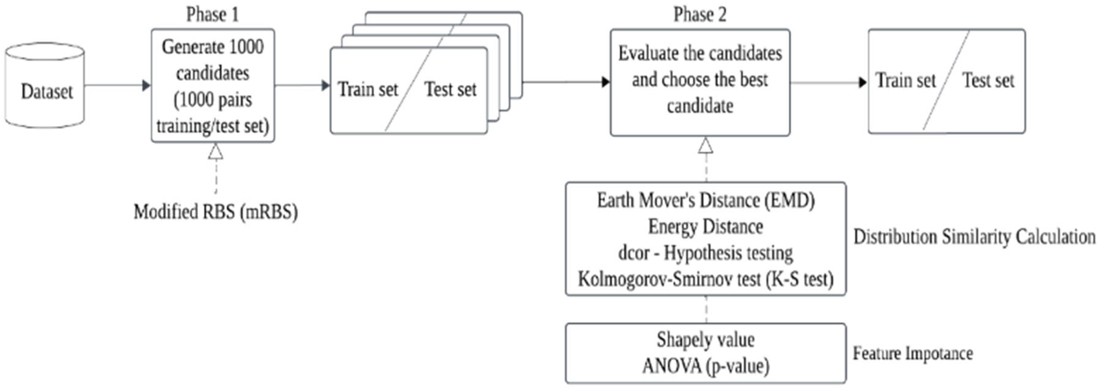
Figure 2.
The process of the proposed sampling method for categorical dataset.
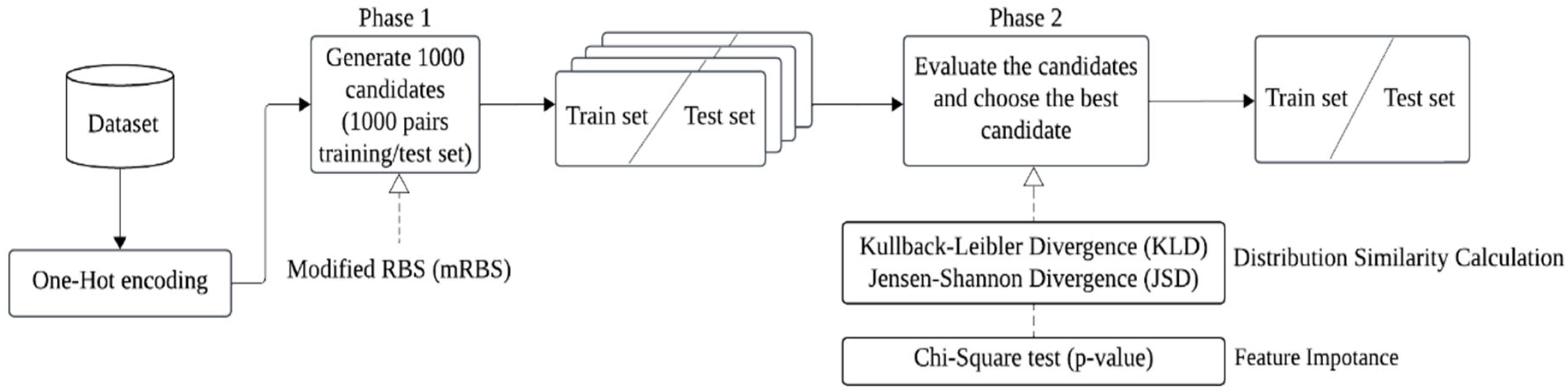

Table 1.
dataset description.
| Dataset | # of instances | # of attributes | # of classes |
| breastcancer | 569 | N:30 | 2 |
| breastTissue | 106 | N:9 | 6 |
| ecoli | 336 | N:7 | 8 |
| pima_diabetes | 768 | N:8 | 2 |
| seed | 218 | N:8 | 3 |
| balance-scale | 625 | C:4 | 3 |
| congressional_voting_records | 435 | C:16 | 2 |
| Qualitative_Bankruptcy | 250 | C:6 | 2 |
| SPEC_Heart | 267 | C:22 | 2 |
| Vector_Borne_ Disease |
263 | C:64 | 11 |
| credit_approval | 690 | N:6, C:9 | 2 |
| Differentiated_Thyroid_Cancer _ Recurrence |
383 | N:1, C:15 | 2 |
| Fertility | 100 | N:3, C:6 | 2 |
| Heart_Disease | 303 | N:5, C:8 | 2 |
| Wholesale_customers _data |
440 | N:6, C:1 | 3 |
Table 2.
the parameters for each classifier.
| Classifier | Parameter |
| Decision Tree (DT) | criterion='entropy', min_samples_leaf=2 |
| Random Forest (RF) | n_estimators=500, max_features='sqrt' |
| K-Nearest Neighbor (KNN) | n_neighbors=5 |
| Support Vector Machine (SVM) | kernel='rbf' |
Table 3.
Average accuracy (AEV) and standard deviation (SD) for each classifiers on numerical datasets.
Table 3.
Average accuracy (AEV) and standard deviation (SD) for each classifiers on numerical datasets.
| Dataset | Classifier | AEV | SD |
| breastcaner | DT | 0.929 | 0.020 |
| KNN | 0.969 | 0.013 | |
| RF | 0.959 | 0.016 | |
| SVM | 0.976 | 0.012 | |
| breastTissue | DT | 0.655 | 0.086 |
| KNN | 0.639 | 0.085 | |
| RF | 0.684 | 0.082 | |
| SVM | 0.549 | 0.075 | |
| ecoli | DT | 0.797 | 0.043 |
| KNN | 0.855 | 0.034 | |
| RF | 0.862 | 0.033 | |
| SVM | 0.864 | 0.035 | |
| pima_diabetes | DT | 0.701 | 0.033 |
| KNN | 0.735 | 0.028 | |
| RF | 0.762 | 0.026 | |
| SVM | 0.767 | 0.027 | |
| seed | DT | 0.907 | 0.039 |
| KNN | 0.929 | 0.033 | |
| RF | 0.924 | 0.036 | |
| SVM | 0.931 | 0.031 |
Table 4.
The accuracy of different distribution distance calculation methods (Shapely value).
| Dataset | Classifier | (FWS)EMD | Energy Distance | dcor-Hypothesis testing | K-S test |
| breastcancer | DT | 0.935 | 0.945 | 0.930 | 0.935 |
| KNN | 0.979 | 0.969 | 0.969 | 0.969 | |
| RF | 0.972 | 0.979 | 0.981 | 0.974 | |
| SVM | 0.979 | 0.979 | 0.979 | 0.979 | |
| breastTissue | DT | 0.739 | 0.703 | 0.703 | 0.714 |
| KNN | 0.679 | 0.679 | 0.643 | 0.714 | |
| RF | 0.760 | 0.725 | 0.689 | 0.714 | |
| SVM | 0.669 | 0.561 | 0.633 | 0.597 | |
| ecoli | DT | 0.812 | 0.765 | 0.800 | 0.812 |
| KNN | 0.824 | 0.847 | 0.835 | 0.824 | |
| RF | 0.847 | 0.882 | 0.835 | 0.847 | |
| SVM | 0.835 | 0.882 | 0.871 | 0.835 | |
| pima_ | DT | 0.705 | 0.731 | 0.694 | 0.705 |
| diabetes | KNN | 0.741 | 0.705 | 0.679 | 0.736 |
| RF | 0.762 | 0.756 | 0.798 | 0.777 | |
| SVM | 0.772 | 0.782 | 0.808 | 0.803 | |
| seed | DT | 0.907 | 0.926 | 0.907 | 0.926 |
| KNN | 0.963 | 0.907 | 0.963 | 0.907 | |
| RF | 0.926 | 0.926 | 0.907 | 0.926 | |
| SVM | 0.963 | 0.907 | 0.926 | 0.944 |
Table 5.
The accuracy of different distribution distance calculation methods (ANOVA).
| Dataset | Classifier | EMD | Energy Distance | dcor-Hypothesis testing | K-S test |
| breastcancer | DT | 0.951 | 0.902 | 0.937 | 0.923 |
| KNN | 0.972 | 0.965 | 0.951 | 0.965 | |
| RF | 0.951 | 0.958 | 0.965 | 0.958 | |
| SVM | 0.972 | 0.972 | 0.972 | 0.972 | |
| breastTissue | DT | 0.500 | 0.714 | 0.643 | 0.750 |
| KNN | 0.607 | 0.643 | 0.607 | 0.714 | |
| RF | 0.643 | 0.750 | 0.679 | 0.679 | |
| SVM | 0.536 | 0.536 | 0.500 | 0.571 | |
| ecoli | DT | 0.812 | 0.824 | 0.765 | 0.835 |
| KNN | 0.823 | 0.894 | 0.882 | 0.847 | |
| RF | 0.859 | 0.894 | 0.847 | 0.871 | |
| SVM | 0.835 | 0.894 | 0.859 | 0.824 | |
| pima_ | DT | 0.731 | 0.710 | 0.710 | 0.710 |
| diabetes | KNN | 0.756 | 0.782 | 0.725 | 0.720 |
| RF | 0.808 | 0.751 | 0.798 | 0.756 | |
| SVM | 0.803 | 0.767 | 0.782 | 0.762 | |
| seed | DT | 0.889 | 0.926 | 0.907 | 0.944 |
| KNN | 0.944 | 0.889 | 0.944 | 0.907 | |
| RF | 0.963 | 0..907 | 0.963 | 0.907 | |
| SVM | 0.926 | 0.907 | 0.926 | 0.907 |
Table 6.
The MAI of different distribution distance calculation methods (Shapely value).
| Dataset | Classifier | (FWS)EMD | Energy Distance | dcor-Hypothesis testing | K-S test |
| breastcancer | DT | 0.286 | 0.748 | 0.059 | 0.286 |
| KNN | 0.918 | 0.139 | 0.139 | 0.139 | |
| RF | 0.818 | 1.253 | 1.356 | 0.921 | |
| SVM | 0.289 | 0.289 | 0.282 | 0.282 | |
| breastTissue | DT | 0.977 | 0.560 | 0.560 | 0.691 |
| KNN | 0.462 | 0.462 | 0.044 | 0.880 | |
| RF | 0.935 | 0.499 | 0.064 | 0.372 | |
| SVM | 1.592 | 0.171 | 1.118 | 0.302 | |
| ecoli | DT | 0.347 | 0.756 | 0.071 | 0.347 |
| KNN | 0.946 | 0.250 | 0.598 | 0.946 | |
| RF | 0.460 | 0.606 | 0.598 | 0.460 | |
| SVM | 0.825 | 0.519 | 0.183 | 0.825 | |
| pima_ | DT | 0.732 | 1.205 | 0.102 | 0.260 |
| diabetes | KNN | 0.228 | 0.978 | 0.710 | 0.603 |
| RF | 0.369 | 0.369 | 1.170 | 1.033 | |
| SVM | 0.962 | 0.013 | 0.013 | 0.182 | |
| seed | DT | 0.020 | 0.490 | 0.020 | 0.490 |
| KNN | 1.039 | 0.655 | 1.039 | 0.655 | |
| RF | 0.047 | 0.047 | 0.463 | 0.047 | |
| SVM | 1.038 | 0.740 | 0.147 | 0.445 | |
| Average | MAI | 0.665 | 0.537 | 0.437 | 0.508 |
Table 7.
The MAI of different distribution distance calculation methods (ANOVA).
| Dataset | Classifier | EMD | Energy Distance | dcor-Hypothesis testing | K-S test |
| breastcancer | DT | 0.286 | 0.631 | 0.403 | 0.286 |
| KNN | 0.668 | 0.668 | 1.196 | 0.918 | |
| RF | 0.487 | 0.052 | 0.383 | 0.487 | |
| SVM | 0.289 | 0.289 | 0.289 | 0.282 | |
| breastTissue | DT | 0.977 | 1.525 | 0.143 | 0.977 |
| KNN | 0.374 | 0.044 | 0.374 | 0.462 | |
| RF | 0.935 | 0.808 | 0.372 | 0.499 | |
| SVM | 0.171 | 0.171 | 0.645 | 0.645 | |
| ecoli | DT | 0.071 | 0.347 | 0.071 | 0.899 |
| KNN | 0.946 | 1.144 | 0.796 | 0.250 | |
| RF | 0.460 | 0.961 | 0.460 | 0.251 | |
| SVM | 0.825 | 0.855 | 0.153 | 1.161 | |
| pima_ | DT | 1.473 | 0.260 | 0.056 | 1.205 |
| diabetes | KNN | 0.148 | 1.728 | 0.603 | 0.148 |
| RF | 1.233 | 0.032 | 0.169 | 0.833 | |
| SVM | 0.989 | 0.013 | 0.767 | 0.989 | |
| seed | DT | 0.450 | 0.490 | 0.020 | 0.020 |
| KNN | 0.474 | 1.220 | 0.474 | 1.039 | |
| RF | 1.067 | 0.463 | 1.067 | 0.557 | |
| SVM | 0.147 | 0.740 | 0.147 | 1.038 | |
| Average | MAI | 0.626 | 0.622 | 0.429 | 0.647 |
Table 8.
Average accuracy (AEV) and standard deviation (SD) of each classifier on categorical datasets.
Table 8.
Average accuracy (AEV) and standard deviation (SD) of each classifier on categorical datasets.
| Dataset | Classifier | AEV | SD |
| balance-scale | DT | 0.745 | 0.034 |
| KNN | 0.744 | 0.030 | |
| RF | 0.845 | 0.026 | |
| SVM | 0.862 | 0.025 | |
| congressional_voting | DT | 0.951 | 0.025 |
| _records | KNN | 0.922 | 0.032 |
| RF | 0.963 | 0.021 | |
| SVM | 0.963 | 0.022 | |
| Qualitative_ | DT | 0.995 | 0.012 |
| Bankruptcy | KNN | 0.996 | 0.008 |
| RF | 0.9995 | 0.005 | |
| SVM | 0.996 | 0.009 | |
| SPEC_Heart | DT | 0.747 | 0.049 |
| KNN | 0.796 | 0.046 | |
| RF | 0.824 | 0.040 | |
| SVM | 0.828 | 0.041 | |
| Vector_Borne | DT | 0.709 | 0.064 |
| _Disease | KNN | 0.673 | 0.057 |
| RF | 0.934 | 0.030 | |
| SVM | 0.914 | 0.037 |
Table 9.
The accuracy of different feature-weighted distance methods on categorical datasets.
| Dataset | Classifier | KLD |
KLD |
JSD | FWS (EMD Shapely) |
| balance-scale | DT | 0.741 | 0.722 | 0.734 | 0.747 |
| KNN | 0.747 | 0.747 | 0.747 | 0.747 | |
| RF | 0.823 | 0.848 | 0.829 | 0.816 | |
| SVM | 0.816 | 0.816 | 0.816 | 0.816 | |
| congressional_ | DT | 0.949 | 0.949 | 0.949 | 0.898 |
| voting _records | KNN | 0.915 | 0.915 | 0.915 | 0.949 |
| RF | 0.983 | 0.983 | 0.983 | 0.966 | |
| SVM | 0.983 | 0.983 | 0.983 | 0.966 | |
| Qualitative_ | DT | 1.000 | 1.000 | 1.000 | 1.000 |
| _Bankruptcy | KNN | 1.000 | 1.000 | 1.000 | 0.984 |
| RF | 1.000 | 1.000 | 1.000 | 1.000 | |
| SVM | 0.984 | 0.984 | 0.984 | 1.000 | |
| SPEC_Heart | DT | 0.716 | 0.716 | 0.761 | 0.761 |
| KNN | 0.776 | 0.776 | 0.776 | 0.821 | |
| RF | 0.776 | 0.791 | 0.791 | 0.791 | |
| SVM | 0.821 | 0.821 | 0.821 | 0.791 | |
| Vector_Borne | DT | 0.761 | 0.761 | 0.776 | 0.761 |
| _Disease | KNN | 0.687 | 0.687 | 0.687 | 0.687 |
| RF | 0.940 | 0.955 | 0.940 | 0.955 | |
| SVM | 0.955 | 0.955 | 0.955 | 0.955 |
Table 10.
The MAI of different feature-weighted distance calculation method on categorical datasets.
Table 10.
The MAI of different feature-weighted distance calculation method on categorical datasets.
| Dataset | Classifier | KLD |
KLD |
JSD | FWS (EMD Shapely) |
| balance-scale | DT | 0.881 | 0.881 | 0.478 | 0.064 |
| KNN | 0.795 | 0.795 | 0.795 | 0.098 | |
| RF | 0.272 | 0.818 | 0.272 | 1.078 | |
| SVM | 0.673 | 0.673 | 0.673 | 1.825 | |
| congressional_ | DT | 0.088 | 0.088 | 0.088 | 2.141 |
| voting _records | KNN | 0.193 | 0.193 | 0.193 | 0.853 |
| RF | 0.974 | 0.974 | 0.974 | 0.165 | |
| SVM | 0.921 | 0.921 | 0.921 | 0.154 | |
| Qualitative_ | DT | 0.474 | 0.474 | 0.474 | 0.474 |
| _Bankruptcy | KNN | 0.548 | 0.548 | 0.548 | 1.503 |
| RF | 0.087 | 0.087 | 0.087 | 0.087 | |
| SVM | 1.335 | 1.335 | 1.335 | 0.467 | |
| SPEC_Heart | DT | 0.626 | 0.626 | 0.286 | 0.286 |
| KNN | 0.429 | 0.429 | 0.429 | 0.536 | |
| RF | 1.193 | 0.817 | 0.817 | 0.817 | |
| SVM | 0.174 | 0.174 | 0.174 | 0.902 | |
| Vector_Borne | DT | 0.806 | 0.806 | 1.039 | 0.806 |
| _Disease | KNN | 0.234 | 0.234 | 0.234 | 0.234 |
| RF | 0.205 | 0.704 | 0.205 | 0.704 | |
| SVM | 1.121 | 1.121 | 1.121 | 1.121 | |
| Average | MAI | 0.601 | 0.635 | 0.557 | 0.716 |
Table 11.
Average accuracy (AEV) and standard deviation (SD) of each classifiers on mix-type datasets.
Table 11.
Average accuracy (AEV) and standard deviation (SD) of each classifiers on mix-type datasets.
| Dataset | Classifier | ACC | SD |
| credit_approval | DT | 0.817 | 0.029 |
| KNN | 0.862 | 0.024 | |
| RF | 0.873 | 0.023 | |
| SVM | 0.862 | 0.023 | |
| Differentiated_ | DT | 0.942 | 0.022 |
| Thyroid_Cancer_ | KNN | 0.922 | 0.027 |
| Recurrence | RF | 0.960 | 0.017 |
| SVM | 0.955 | 0.019 | |
| Fertility | DT | 0.846 | 0.064 |
| KNN | 0.853 | 0.055 | |
| RF | 0.869 | 0.057 | |
| SVM | 0.881 | 0.057 | |
| Heart_Disease | DT | 0.749 | 0.048 |
| KNN | 0.829 | 0.038 | |
| RF | 0.822 | 0.038 | |
| SVM | 0.839 | 0.037 | |
| Wholesale_customers | DT | 0.524 | 0.045 |
| _data | KNN | 0.635 | 0.037 |
| RF | 0.709 | 0.036 | |
| SVM | 0.718 | 0.037 |
Table 12.
MAI and test accuracy for mix-type datasets.
| Dataset | Classifier | Our hybrid method (Accuracy) |
dcor-Hypothesis testing ANOVA (Accuracy) |
Our hybrid method (MAI) | dcor-Hypothesis testing ANOVA (MAI) |
| credit_approval | DT | 0.793 | 0.768 | 0.828 | 1.669 |
| KNN | 0.896 | 0.896 | 1.414 | 1.414 | |
| RF | 0.854 | 0.866 | 0.867 | 0.329 | |
| SVM | 0.854 | 0.854 | 0.376 | 0.376 | |
| Differentiated_ | DT | 0.938 | 0.938 | 0.189 | 0.189 |
| Thyroid_Cancer_ | KNN | 0.938 | 0.938 | 0.596 | 0.596 |
| Recurrence | RF | 0.948 | 0.948 | 0.699 | 0.699 |
| SVM | 0.938 | 0.938 | 0.910 | 0.910 | |
| Fertility | DT | 0.885 | 0.885 | 0.610 | 0.610 |
| KNN | 0.808 | 0.808 | 0.820 | 0.820 | |
| RF | 0.846 | 0.846 | 0.398 | 0.398 | |
| SVM | 0.885 | 0.885 | 0.059 | 0.059 | |
| Heart_Disease | DT | 0.792 | 0.805 | 0.903 | 1.172 |
| KNN | 0.870 | 0.870 | 1.085 | 1.085 | |
| RF | 0.857 | 0.857 | 0.918 | 0.918 | |
| SVM | 0.857 | 0.857 | 0.486 | 0.486 | |
| Wholesale_ | DT | 0.495 | 0.514 | 0.633 | 0.228 |
| customers _data | KNN | 0.676 | 0.676 | 1.105 | 1.105 |
| RF | 0.712 | 0.703 | 0.096 | 0.152 | |
| SVM | 0.739 | 0.739 | 0.558 | 0.558 | |
| Average | MAI | 0.678 | 0.689 |
Disclaimer/Publisher’s Note: The statements, opinions and data contained in all publications are solely those of the individual author(s) and contributor(s) and not of MDPI and/or the editor(s). MDPI and/or the editor(s) disclaim responsibility for any injury to people or property resulting from any ideas, methods, instructions or products referred to in the content. |
© 2025 by the authors. Licensee MDPI, Basel, Switzerland. This article is an open access article distributed under the terms and conditions of the Creative Commons Attribution (CC BY) license (http://creativecommons.org/licenses/by/4.0/).
Copyright: This open access article is published under a Creative Commons CC BY 4.0 license, which permit the free download, distribution, and reuse, provided that the author and preprint are cited in any reuse.


