Highland Areas in the Digital Era: From Abyss to Quatum: European Mountain Series Analysis (10)

1. Introduction and Literature Review

Predominantly due to isolation and marginalization, highland areas display particular characteristics across all sectors of the national economy, but especially in the field of digitalization. Numerous studies on the sustainability of digitalization in mountain regions have focused on the dynamics of informational resources and networks.

A study on digitalization in one of the poorest regions of Peru, located in the high Andes, shows that information and communication technologies (ICTs) are developing new flows that were almost impossible before their impact on human development. Two of the most resilient groups in adopting ICT are young farmers and school-aged children. In mountainous areas, agriculture is heavily impacted by ICT, as is the education system. The creation of telecenters has elevated human development in highland areas to a new level. Through ICT, the intangible becomes tangible, inaccessibility becomes accessibility, untimeliness becomes opportunity, and so on. For this reason, ICT is increasingly seen in these areas as a new way to address the challenge of human development in mountain regions. (Heeks & Kanashiro, 2009)

Another study on mountain areas identifies ICT implementation as one of the most important regenerative factors. Development occurs not only in already populated mountain regions but also in those with future settlement potential. Especially amid global warming and climate change, mountain areas will become increasingly necessary in the coming decades. Extreme phenomena in lowland areas, such as drought or sharply rising sea levels, will push segments of the population to higher elevations. In this context, challenges related to communication, overexploitation of resources, environmental pollution, and disruption of local livelihoods will intensify. On the other hand, if mountain regions are properly managed, these challenges can be transformed into development opportunities: creating jobs, improving access to services and global integration, and strengthening supply-distribution chains. Another key to ensuring the resilience of highland zones is energy development. ICT significantly improves access to current energy sources, such as active solar, wind, and passive solar energy. Transportation and construction infrastructure—traditionally weak in mountainous areas—has seen considerable improvements in the past decade, a trend that is likely to continue. More than in other areas, specific transport technologies—such as cable cars, suspension bridges, or aerial transport—offer effective solutions for mountain isolation. ICT has proven its potential across all development sectors, with a decisive influence on mountain development. The development of communications requires coordinated efforts from local, regional, national, and transnational public/private governance.

By their very nature, mountains are more or less dependent on the networks of other terrain types. Industrialization brought about the need for technology, and subsequently for digitalization, in mountain areas. This trend was amplified by successive waves of economic development, making digitalization an imperative today. Mountain areas follow the same rules as other regions, but their resilient impact is harder to predict. Current digital technologies have recently found coherent applications, whereas until recently, digitalization's impact on mountainous regions was minimal. The introduction of the Internet of Things, and especially 5G technologies, has marked a turning point in the digital development of mountain regions.

Digitalization in mountain areas also has another dimension: the migration of the skilled population capable of applying new technologies. Therefore, mountain societies—often characterized by an aging population—must undergo a greater technological and cognitive leap than other societies. The digital pressure demands profound societal transformations in mountain areas, which could prove beneficial for the sustainability and renewable development of highland regions. However, on a global scale, digitalization in mountain areas remains highly uneven. There are still few properly digitalized mountain zones, while most highland regions around the world exhibit low levels of technological integration. The focal point of mountain development will lie in the capacity to technologize and digitalize these areas. (Kohler et al., 2004)

Another study on mountain regions emphasizes the importance of telecommunications infrastructure services. The sparse population in certain mountain zones, coupled with the unfavorable cost-benefit ratio of installing technologies, currently hinders the proper implementation of digitalization. A significant aspect of mountain demographics is the disproportionate number of women, children, and the elderly, due to the seasonal migration of men for work. The population that remains—overburdened with survival responsibilities—does not invest financial gains in technology, prioritizing other urgent human needs such as food, safety, and clothing. These are primary and secondary sector needs; only afterward are tertiary and quaternary needs addressed. Digitalization, as part of the quaternary sector, is not an immediate necessity for many mountain populations. This applies even when the cost-benefit ratio clearly favors digitalization, mainly due to poor awareness of its advantages. From Thailand to Bolivia, Uganda to Nepal, and India to Ecuador, the stories of new ICTs highlight real differences in people’s lives. However, change in mountain areas happens slowly. (Aitkin, 2002)

Ensuring the safety of mountain populations is also vital. New information technologies enable faster warnings about potential dangers. Therefore, dynamic early warning models and their standardization are becoming essential. Additionally, it is necessary to assess the current state of development and digitalization practices. One of the most important digital technologies is big data, primarily used to enhance efficiency and improve predictive value. (He et al., 2017)

A marginal, yet highly sustainable, aspect of mountain digitalization is the opportunity for knowledge sharing and network creation through ICTs. In countries with sustained political instability and weak governance, the absence of digitalization—alongside harsh natural conditions—poses significant constraints to human safety. Possible ways to overcome these major obstacles involve knowledge sharing and networking enabled by ICT. In this context, some authors propose new facilitation methods for creating networks and sharing knowledge to ensure the Sustainable Development of Mountain Areas through ICT. Partnerships between various mountain regions with different development levels offer a real solution for both, particularly for disadvantaged areas. More developed mountain regions expand their networks of influence, while underdeveloped ones enhance their development levels. This win-win outcome is seen as the paradigm for such collaborations. (Dzhusupova & Aidaraliev, 2011)

Mountain region subsistence is supported primarily through the primary and secondary sectors of the economy, but sustainable efficiency is achieved through the tertiary and quaternary sectors. Tourism, the most important source of income in mountain areas, relies heavily on information and communication. Management actions in recreational tourism, ecological education, visitor information, and public relations are integral to the emerging mountain society. The rise of modern ICTs has completely transformed the way information is shared, communication occurs, and data content is accessed. Today, communication processes are closely tied to the use of Web 2.0 tools, which function on computers and mobile devices. This presents unique and innovative opportunities for information and communication activities. These benefits and challenges of modern ICTs are also relevant for large protected areas and should be considered. To efficiently use and integrate modern ICT in mountain activities, specific concepts related to learning, audience targeting, and social integration must be considered. (Hennig et al., 2013)

A study on the impact of introducing ICT in mountainous regions shows that mountain populations, more resistant to change than others, adopt technology more slowly. The "parachute approach"—imposing a technology on an unprepared population—can sometimes worsen the situation. This is why technological education must precede its actual application. If this rule is not followed, a new paradox may arise: the "parasite approach," where the population rejects technology as useless. Mountain populations follow the same psychological rules, which is why introducing technology must be preceded by education focused on digital readiness. (Okada & Hatayama, 2002)

A study on rural mountain regions in New Zealand highlights the importance of ICT in connecting communities with tourism. In small communities, ICT effectiveness has multiple advantages, the most significant being the development of tourism. Due to its deeply practical nature in mountain societies, tourism should be viewed not only as an extension of the tertiary sector but also as a support for all economic sectors. Both financially and logistically, tourism—in its agro-forestry-pastoral, industrial, service-based, and quaternary forms—supports the entire economic structure of a mountain region. (Deuchar & Milne, 2016)

In all mountain communities, ICT helps create or strengthen social capital, which in turn drives development. Recent research in Nepal on wireless technology supports the importance of digitalization in expanding social capital and socio-economic development. These studies also examined the social dimension of digitalization among local populations, finding that social phenomena like bridging, bonding, and linking are more easily achieved through ICT. In a dynamic society, such social phenomena ensure the sustainability of all dimensions of mountain existence. ICT plays a decisive role in addressing numerous challenges faced in mountain life, such as high illiteracy rates, poor physical infrastructure, and language barriers. (Thapa & Sein, 2010)

Another facet of human existence in the technological context is the control and prevention of climate change effects. Web interfaces connect data from various sources and integrate them with near-real-time climate and meteorological datasets, providing updated environmental information. Digital systems offer vital information in mountain environments, such as land use conditions, adaptation options, and near real-time data on precipitation and temperatures. (Khezri et al., 2018)

2. Methodology

2.1. Research Purpose and General Context

This research analyzes the evolution of key indicators related to firm dynamics, survival, employment, and mobility in the business environment for the period 2021–2022, using statistical data structured around 28 relevant economic indicators from information and communication technology entrepreneurship. The study focuses on a comparative assessment between the two years, aiming to identify trends and fluctuations in the demographic structure of firms and developments related to employment and growth.

The data was organized in the form of 28 statistical indicators from Eurostat (labeled I1 to I28) for each of the years 2021 and 2022 (tables and figures). These indicators reflect both quantitative aspects (e.g., number of newly established enterprises, number of employees) and percentage rates (e.g., enterprise survival rate, employment growth rate). The detailed structure of each indicator is presented in the accompanying significance table, following standardized definitions of European statistics in the fields of entrepreneurship and labor markets.

	I1.2021			I1.2022				I2.2021			I2.2022				I3.2021		I3.2022			I4.2021		I4.2022			I5.2021		I5.2022			I6.2021				I6.2022		I7.2021			I7.2022			I8.2021				I8.2022
N Valid	15			12				13			11				10		8			13		11			13		11			8				8		12			11			12				11
N Missing	0			3				2			4				5		7			2		4			2		4			7				7		3			4			3				4
Mean	14780.80			14802.50				1803.00			2056.91				1.0040		1.0225			1.00		1.00			1107.46		1417.18			24.0763				20.4938		761.58			1007.27			6.8133				6.6945
Std. Error of Mean	3678.344			3840.639				513.320			576.636				0.10861		0.15454			0.000		0.000			340.115		377.696			12.26552				11.98987		193.963			261.008			0.58107				0.53648
Median	9870.00			11755.50				1053.00			1264.00				1.0500		1.0350			1.00		1.00			678.00		730.00			9.2700				8.0750		605.50			684.00			6.6800				7.6200
Mode	581a			508a				41a			46a				1.19		.43a			1		1			25a		23a			1.34a				.95a		32a			22a			4.02a				3.66a
Std. Deviation	14246.166			13304.362				1850.801			1912.484				0.34345		0.43709			0.000		0.000			1226.303		1252.674			34.69213				33.91247		671.906			865.665			2.01290				1.77930
Skewness	1.574			1.791				1.828			1.373				0.509		0.522								2.063		0.833			2.277				2.664		1.715			1.071			0.313				-0.550
Std. Error of Skewness	0.580			0.637				0.616			0.661				0.687		0.752			0.616		0.661			0.616		0.661			0.752				0.752		0.637			0.661			0.637				0.661
Kurtosis	1.557			3.417				2.863			1.336				0.756		0.826								3.702		-0.896			5.412				7.274		3.892			0.205			-0.806				-1.087
Std. Error of Kurtosis	1.121			1.232				1.191			1.279				1.334		1.481			1.191		1.279			1.191		1.279			1.481				1.481		1.232			1.279			1.232				1.279
Range	46492			48177				6465			6302				1.16		1.40			0		0			4283		3414			103.66				102.19		2491			2584			6.47				5.41
Minimum	581			508				41			46				0.54		0.43			1		1			25		23			1.34				0.95		32			22			4.02				3.66
Maximum	47073			48685				6506			6348				1.70		1.83			1		1			4308		3437			105.00				103.14		2523			2606			10.49				9.07
Sum	221712			177630				23439			22626				10.04		8.18			13		11			14397		15589			192.61				163.95		9139			11080			81.76				73.64
Percentiles 25	6025.00			7496.25				792.00			932.00				0.6900		0.6325			1.00		1.00			453.50		562.00			4.7700				4.9750		309.50			444.00			5.3700				5.1300
Percentiles 50	9870.00			11755.50				1053.00			1264.00				1.0500		1.0350			1.00		1.00			678.00		730.00			9.2700				8.0750		605.50			684.00			6.6800				7.6200
Percentiles 75	14680.00			15919.25				2256.50			3384.00				1.1900		1.2550			1.00		1.00			1079.50		2832.00			32.8675				18.5475		1116.25			1287.00			8.2900				7.8100
a. Multiple modes exist. The smallest value is shown
	I10.2021		I10.2022				I12.2021			I12.2022			I13.2021			I13.2022				I14.2021			I14.2022			I15.2022		I16.2021			I16.2022				I17.2021			I17.2022			I18.2021				I18.2022
N Valid	13		10				13			11			13			11				13			11			12		14			12				10			8			9				8
N Missing	2		5				2			4			2			4				2			4			3		1			3				5			7			6				7
Mean	75.08		70.50				22.5792			23.1073			14.2931			13.6618				8.2877			9.4473			6.5350		56947.29			55328.42				1892.30			1882.38			5.8378				5.4563
Std. Error of Mean	19.701		27.064				2.27403			2.31327			1.59912			1.37452				0.75385			1.44611			2.08971		17949.140			16558.386				471.384			539.182			1.15044				1.30930
Median	48.00		36.50				20.7600			25.1900			12.4900			12.6500				7.7700			8.8000			7.6050		30867.00			33376.00				1453.00			1643.50			6.4600				4.5000
Mode	20		3a				11.36a			13.58a			7.04a			7.67a				4.30a			4.53a			-12.56a		978a			918a				30a			20a			2.27a				2.18a
Std. Deviation	71.032		85.585				8.19912			7.67226			5.76573			4.55876				2.71803			4.79620			7.23898		67159.532			57359.932				1490.649			1525.038			3.45133				3.70326
Skewness	0.799		1.475				0.522			-0.019			0.374			0.213				1.071			1.814			-1.715		1.679			1.358				0.415			0.285			0.497				0.672
Std. Error of Skewness	0.616		0.687				0.616			0.661			0.616			0.661				0.616			0.661			0.637		0.597			0.637				0.687			0.752			0.717				0.752
Kurtosis	-0.570		0.765				-0.809			-1.822			-1.318			-1.520				1.390			4.216			4.113		1.890			1.025				-1.433			-1.672			-0.910				-0.929
Std. Error of Kurtosis	1.191		1.334				1.191			1.279			1.191			1.279				1.191			1.279			1.232		1.154			1.232				1.334			1.481			1.400				1.481
Range	204		233				25.36			20.76			16.65			12.73				10.33			17.24			27.70		217313			184498				4204			4041			9.64				9.63
Minimum	1		3				11.36			13.58			7.04			7.67				4.30			4.53			-12.56		978			918				30			20			2.27				2.18
Maximum	205		236				36.72			34.34			23.69			20.40				14.63			21.77			15.14		218291			185416				4234			4061			11.91				11.81
Sum	976		705				293.53			254.18			185.81			150.28				107.74			103.92			78.42		797262			663941				18923			15059			52.54				43.65
Percentiles 25	16.50		13.75				16.9500			15.9600			9.6250			9.1200				6.6650			6.0100			3.7600		11129.75			13156.75				539.50			536.50			2.5350				2.2375
Percentiles 50	48.00		36.50				20.7600			25.1900			12.4900			12.6500				7.7700			8.8000			7.6050		30867.00			33376.00				1453.00			1643.50			6.4600				4.5000
Percentiles 75	121.00		119.25				29.5050			30.1000			20.1350			17.8200				9.6600			10.7000			11.2900		67894.50			102870.75				3454.25			3439.75			8.5950				8.4825
a. Multiple modes exist. The smallest value is shown
		I19.2021				I19.2022			I20.2021					I20.2022					I21.2021		I21.2022					I22.2021			I22.2022				I23.2021			I23.2022				I24.2021				I24.2022
N Valid		8				8			9					8					9		8					8			8				9			8				9				8
N Missing		7				7			6					7					6		7					7			7				6			7				6				7
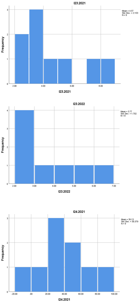
Mean		955.38				1649.38			1249.78					1288.50					887.56		919.13					3.4450			3.7125				4.5667			3.7675				39.1322				22.8063
Std. Error of Mean		404.880				619.696			444.635					509.773					264.743		295.117					0.60128			0.71987				0.71765			0.60158				10.12623				11.89098
Median		556.00				1137.50			956.00					780.00					698.00		653.50					3.0500			2.9900				3.8600			3.0500				34.3800				22.2000
Mode		22a				15a			43a					21a					32a		35a					1.67a			1.63a				2.45a			2.17a				-9.83a				-40.00a
Std. Deviation		1145.173				1752.765			1333.904					1441.856					794.229		834.716					1.70068			2.03610				2.15296			1.70154				30.37870				33.63277
Skewness		2.173				1.096			1.983					1.898					1.010		1.030					0.974			0.725				1.049			0.726				0.086				-0.273
Std. Error of Skewness		0.752				0.752			0.717					0.752					0.717		0.752					0.752			0.752				0.717			0.752				0.717				0.752
Kurtosis		5.132				-0.317			4.480					4.007					0.478		0.465					0.289			-0.726				-0.248			-1.413				-0.423				2.136
Std. Error of Kurtosis		1.481				1.481			1.400					1.481					1.400		1.481					1.481			1.481				1.400			1.481				1.400				1.481
Range		3581				4629			4392					4492					2436		2478					4.97			5.61				5.83			4.21				93.68				119.59
Minimum		22				15			43					21					32		35					1.67			1.63				2.45			2.17				-9.83				-40.00
Maximum		3603				4644			4435					4513					2468		2513					6.64			7.24				8.28			6.38				83.85				79.59
Sum		7643				13195			11248					10308					7988		7353					27.56			29.70				41.10			30.14				352.19				182.45
Percentiles 25		311.00				346.00			358.00					355.25					237.50		272.75					2.0550			1.8625				2.8950			2.3250				17.0400				12.0700
Percentiles 50		556.00				1137.50			956.00					780.00					698.00		653.50					3.0500			2.9900				3.8600			3.0500				34.3800				22.2000
Percentiles 75		1236.50				3406.75			1681.00					1740.75					1507.00		1498.25					4.7075			5.3700				6.4850			5.6625				66.5350				40.9900
a. Multiple modes exist. The smallest value is shown
					I25.2021							I25.2022						I26.2021						I26.2022			I27.2021					I27.2022					I28.2021						I28.2022
N Valid					12							9						7						6			6					7					7						6
N Missing					3							6						8						9			9					8					8						9
Mean					49918.33							41031.33						363.86						490.83			295.67					274.86					27.8386						25.4667
Std. Error of Mean					18110.781							17427.493						136.767						263.686			151.323					201.406					6.40979						7.87423
Median					19032.50							16728.00						194.00						237.00			138.00					90.00					30.2800						18.0750
Mode					696a							710a						17a						4a			0a					3a					5.61a						4.29a
Std. Deviation					62737.586							52282.479						361.851						645.896			370.665					532.870					16.95870						19.28785
Skewness					1.493							1.435						1.178						1.847			1.623					2.554					0.529						0.653
Std. Error of Skewness					0.637							0.717						0.794						0.845			0.845					0.794					0.794						0.845
Kurtosis					1.265							0.664						0.492						3.435			2.315					6.618					0.152						-1.684
Std. Error of Kurtosis					1.232							1.400						1.587						1.741			1.741					1.587					1.587						1.741
Range					192905							142173						1003						1720			979					1470					51.06						46.55
Minimum					696							710						17						4			0					3					5.61						4.29
Maximum					193601							142883						1020						1724			979					1473					56.67						50.84
Sum					599020							369282						2547						2945			1774					1924					194.87						152.80
Percentiles 25					5881.00							4728.00						97.00						66.25			47.25					13.00					15.9200						11.2050
Percentiles 50					19032.50							16728.00						194.00						237.00			138.00					90.00					30.2800						18.0750
Percentiles 75					91304.25							80876.50						674.00						923.00			586.75					204.00					38.3100						48.7175
a. Multiple modes exist. The smallest value is shown

2.2. Type of Data and Sources

The data used in the study is quantitative, originating from a statistically aggregated European-level database. The dataset includes both absolute values (e.g., number of enterprises) and derived metrics (e.g., the ratio of newly established to active enterprises, expressed as a percentage). Each indicator is represented for both analyzed years (2021 and 2022), enabling a comparative evolutionary analysis.

Each variable was analyzed based on the following descriptive parameters: number of valid and missing observations (N Valid and N Missing), mean, standard error of the mean, median, mode, standard deviation, skewness, and kurtosis, along with minimum, maximum, and percentile values (25th, 50th, 75th).

2.3. Data Processing and Statistical Analysis

The data was processed using IBM SPSS Statistics software, version 28. In the descriptive analysis, the distribution of each indicator for the two years was characterized, highlighting measures of central tendency (mean, median), dispersion (standard deviation, range), and distribution shape (skewness and kurtosis).

To assess the evolution between 2021 and 2022, paired mean comparisons were applied for each indicator (where data allowed), testing the statistical significance of differences using the paired samples t-test. For variables that did not follow a normal distribution (as confirmed by significant skewness or high kurtosis), the non-parametric Wilcoxon signed-rank test was used.

Additionally, to identify potential relationships between the analyzed indicators (e.g., between business birth rate and employee growth), Pearson and Spearman correlation analyses were conducted, depending on the variable distribution.

2.4. Handling Missing and Extreme Values

Regarding missing values, these varied across indicators, from 0 to 9 missing observations. A listwise deletion approach was chosen for comparative and inferential analyses to maintain dataset consistency. Missing values were not imputed, as the total number of observations per indicator was relatively low (maximum 15).

To identify and handle outliers, a visual inspection of minimum and maximum values, as well as the interquartile range, was conducted. Indicators I1, I10, I16, and I25 showed significantly higher maximum values than the rest of the distribution; these values were retained in the analysis but discussed separately in the interpretation of results to avoid distorting overall conclusions.

2.5. Methodological Limitations

The dataset, being cross-sectional, covers only two consecutive years (2021 and 2022), which limits the ability to draw long-term trend conclusions. Furthermore, the small number of valid observations in some cases (fewer than 10) restricts the applicability of inferential tests and reduces statistical power. This is particularly relevant for indicators such as I26–I28, where large variation and small sample size can affect the robustness of conclusions.

It is also important to note that the lack of qualitative information (e.g., business sector, geographic region, level of digitalization of firms) may limit the complexity of result interpretation, which is focused exclusively on the numerical and structural dimensions of firms.

2.6. Ethics and Transparency

The analysis was conducted in accordance with ethical principles of scientific research, with all data anonymized and aggregated, making it impossible to identify individual entities. Additionally, all data sources used are public and were handled with care to ensure the reproducibility of the research.

Countries: Portugal, Austria, Germany, Sweden, Spain, Slovenia, Bulgaria, Greece, Romania, Czech Republic, Slovakia, France, Poland, Italy – [https://doi.org/10.5281/zenodo.14713867]

3. Results

3.1. Firm Dynamics: Establishments, Closures, and the Evolution of the Business Population

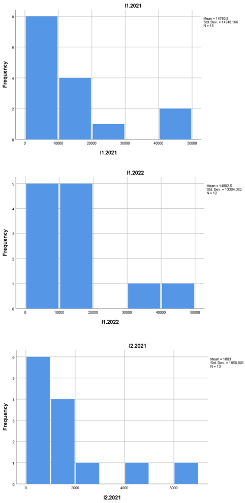
The total number of active enterprises (I1) showed a slight increase, from an average of 14,780.80 in 2021 to 14,802.50 in 2022, indicating overall stability in the entrepreneurial environment. However, this average hides a high dispersion of data (standard deviation over 13,000 in both years), suggesting a strongly skewed distribution, confirmed by positive skewness coefficients (1.574 in 2021, 1.791 in 2022) and kurtosis values above 1 (tables and figures).

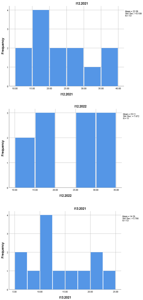
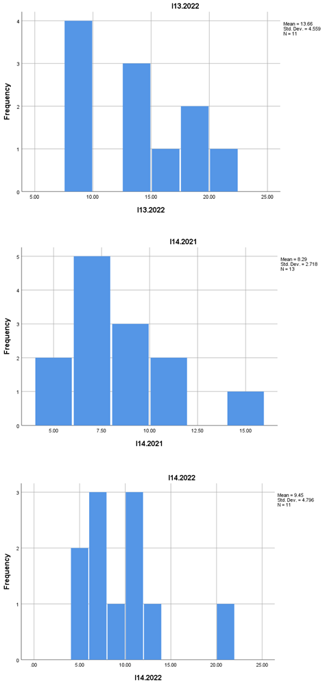
The number of newly established enterprises (I2) also increased, from an average of 1,803 in 2021 to 2,056.91 in 2022. This positive trend is accompanied by a slight decrease in the average business birth rate (I13), from 14.29% in 2021 to 13.66% in 2022. While this may seem like a small drop, it's important to note that the dispersion of this indicator is significant, reflecting important variations between regions or sectors (standard deviation \~5.7 in 2021 and \~4.5 in 2022).

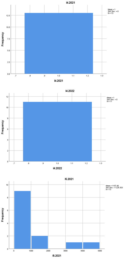
On the other hand, the average number of enterprises exiting the market (I5) increased from 1,107.46 to 1,417.18, accompanied by high variation (standard deviation over 1,200 in both years), indicating high volatility in firm dynamics. The death rate (I14) also rose, from 8.29% to 9.45%, signaling increased pressure on firm survival in 2022.

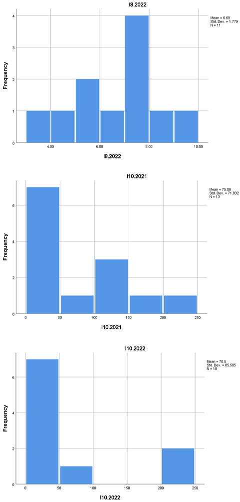
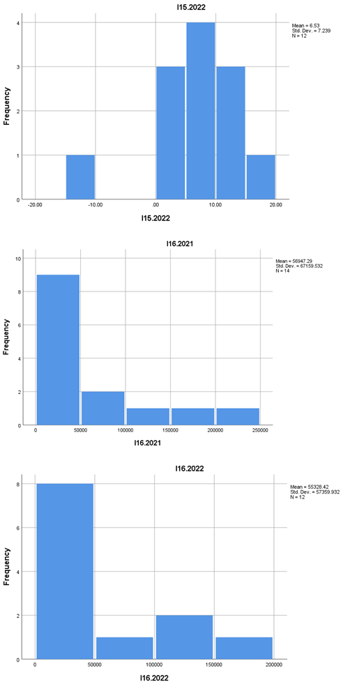
Although both the number of establishments and closures increased, the net population growth rate of enterprises (I15) remained relatively constant (6.81% in 2021 vs. 6.69% in 2022), suggesting a balance between market entries and exits, as well as potential stagnation in the entrepreneurial environment.

3.2. Medium-Term Survival and Enterprise Size

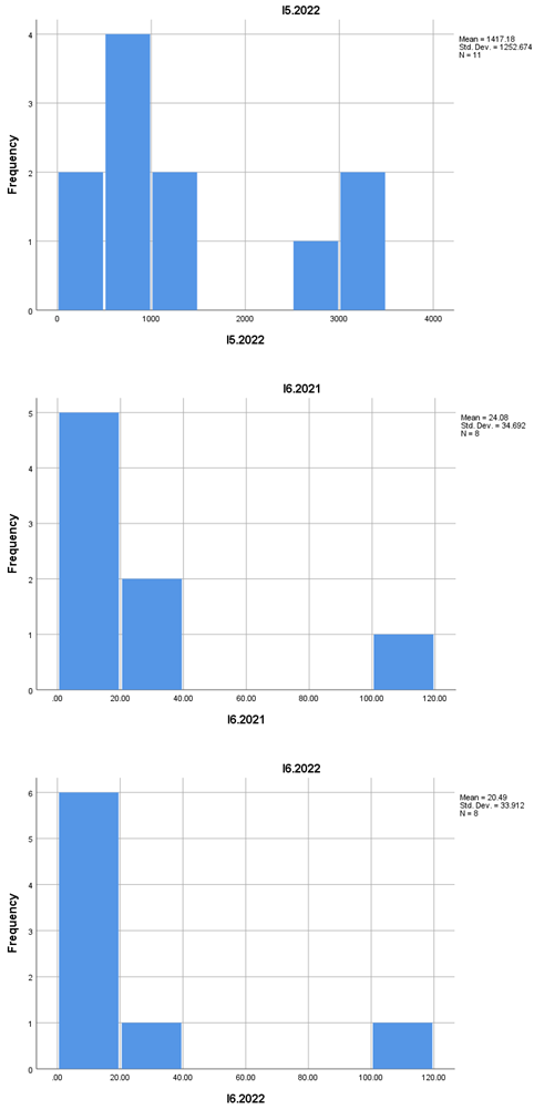
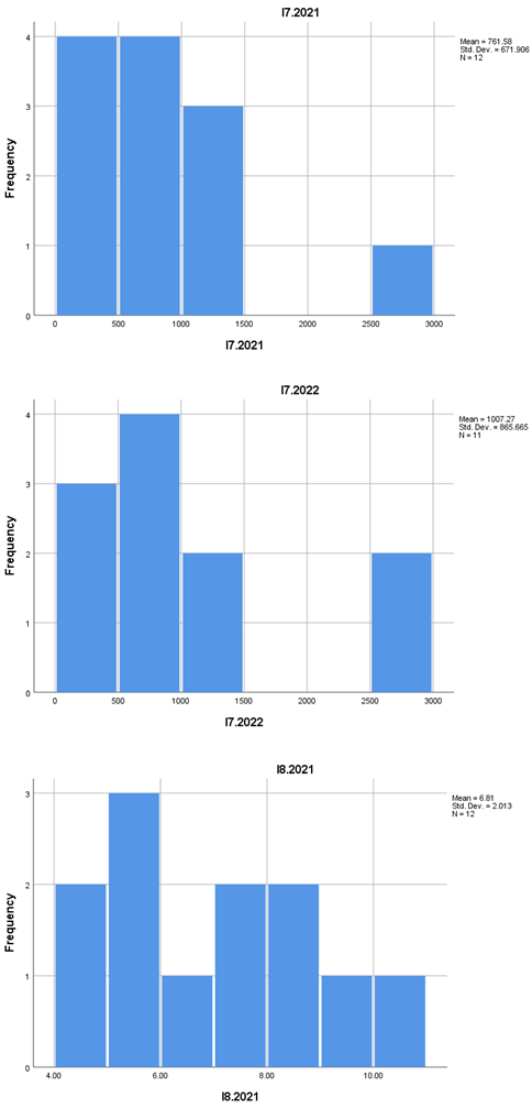
The three-year survival of enterprises (I7) showed a slight decrease in 2022 (from an average of 12 to 11 surviving enterprises), while the survival rate (I9) decreased from 75.08% to 70.50%. This minor drop could indicate slightly worsening market conditions for new businesses. At the same time, the size of newly established firms (I3) increased slightly from 1.004 to 1.022 persons per firm, suggesting a modest trend toward early-stage professionalization.

The average size of firms that survived three years (I6) slightly declined, from 24.07 in 2021 to 20.49 in 2022. This drop, along with a high standard deviation (over 33), suggests that despite surviving, firms did not significantly grow their staff over time—potentially reflecting challenges in scaling or a cautious economic environment.

3.3. Employment Trends in Enterprises

The total number of people employed in enterprises (I16) slightly decreased from an average of 56,947 in 2021 to 55,328 in 2022. The decline may seem modest, but the very high standard deviations (over 57,000) indicate a highly unequal distribution across observed units. It's likely that a few enterprises employ a disproportionately large number of people, while others remain very small.

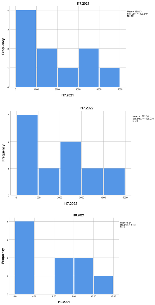
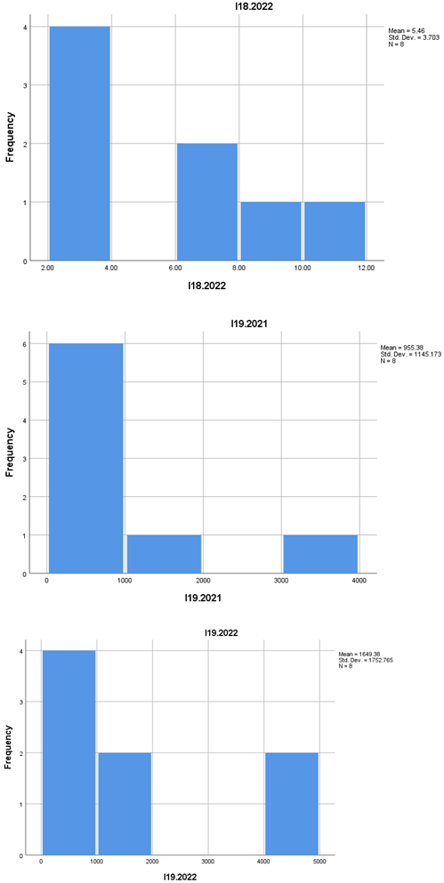
Regarding employees in newly established enterprises (I17), their number remained almost constant (1,892 in 2021 vs. 1,882 in 2022), which could indicate a stabilization in this segment. However, the share of employment in new enterprises (I18) slightly declined from 5.83% to 5.45%, suggesting their contribution to overall employment has marginally decreased.

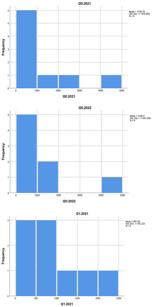
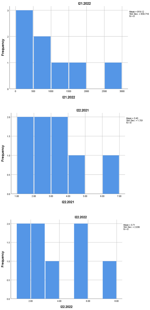
The number of employees in closed enterprises (I19) nearly doubled, from an average of 955 in 2021 to 1,649 in 2022, signaling a greater labor market impact from business closures. Meanwhile, employment in surviving enterprises (I20) remained constant (\~1,250 employees), and those employed in these firms in their founding year (I21) represented a stable segment (\~900 people).

3.4. Enterprise Growth and Performance Indicators

The number of high-growth enterprises in terms of employment (I10) remained relatively stable, around 13 in 2021 and 10 in 2022, while their share among all enterprises with more than 10 employees (I11) averaged 22.5% in 2022, compared to 24.1% in 2021. This slight decrease may reflect a decline in economic dynamism.

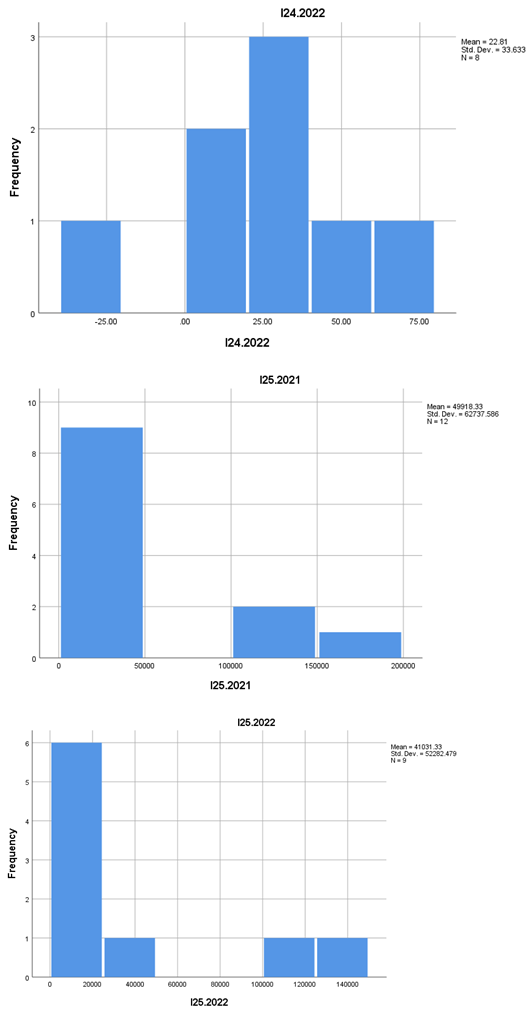
Indicator I24 (employment growth rate in surviving firms) dropped significantly, from 39.1% in 2021 to just 22.8% in 2022. This decline is notable as it reflects a reduced expansion potential even among “survivor” firms, which are generally considered more stable and with growth prospects.

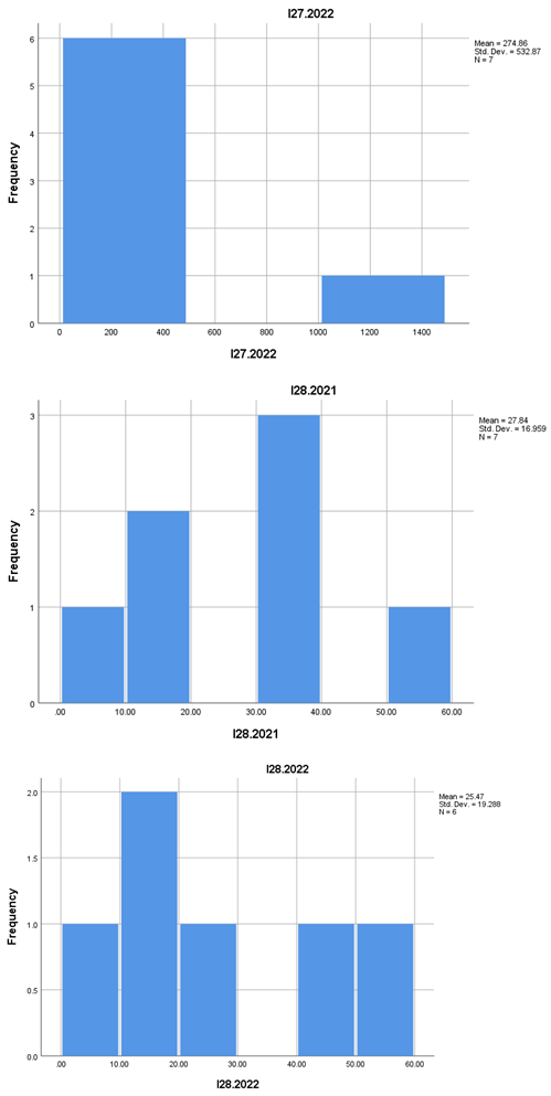
Likewise, the paid employment rate in newly established enterprises (I28) slightly declined from 27.8% to 25.4%, indicating that some of these firms operated in informal conditions or had limited contractual staff resources.

3.5. Fluctuations in the Workforce and Short-Term Effects

Data on the total number of employees (I25) show a drop in the average from 49,918 in 2021 to 41,031 in 2022—a significant difference that suggests a possible reduction in total workforce, either due to firm closures or internal restructuring.

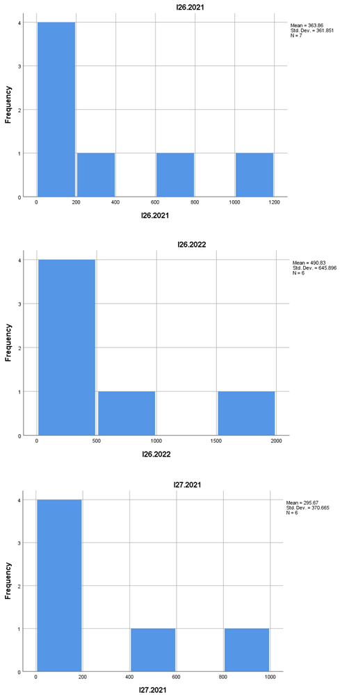
In addition, the number of employees in newly established firms (I26) increased from 363 to 490, which may indicate an effort by new firms to better organize and formally employ staff from the start. On the other hand, employees in closed firms (I27) were fewer on average in 2022 compared to 2021 (decline from 295 to 274), possibly meaning that these firms had relatively few employees at the time of closure.

The results highlight a series of contrasting trends in entrepreneurial dynamics during 2021–2022: a slight increase in new firm establishments but also in closures; stability in net growth rate but a decline in survival rate; a slight reduction in the total workforce, but attempts at strengthening new businesses. Performance indicators point to stagnation or even regression in employment growth, despite apparent resilience in the creation of new economic entities.

4. Discussion and Interpretations

The results provide a detailed picture of enterprise dynamics during the post-pandemic period 2021–2022, a time marked by economic uncertainty, inflationary pressures, and structural readjustments across numerous sectors. The statistical analysis of 28 relevant indicators highlights a series of significant aspects with direct implications for the business environment and public policy (tables and figures).

4.1. A fragile Balance Between Firm Births and Closures

The increase in the number of newly established enterprises, combined with an even more pronounced increase in the number of business closures, reflects an entrepreneurial environment characterized by volatility. Indicators I2 (births) and I5 (deaths) suggest a dynamic process of market entries and exits, typical of a post-crisis transitional economy. Although the average total number of enterprises (I1) remained relatively stable, which may be interpreted as a macro-level equilibrium, the internal dynamics show accelerated turnover, which could become problematic in the long run.

The simultaneous rise in establishment and closure indicators may be attributed to an economic “reset” effect, where unviable businesses exit the market, making room for new initiatives better adapted to current market conditions. However, the fact that the net growth rate (I15) remained relatively constant around 6.8% suggests the economic system has limited capacity to absorb new entrepreneurial capital.

4.2. Slight Decline in Business Resilience

A concerning observation is the drop in the three-year survival rate (I9) and the slight decrease in the average number of firms that manage to survive this critical threshold (I7). These data suggest a weakening ability of newly founded firms to remain viable in the market. While the average size of these firms at founding (I3) increased marginally, this change does not seem to translate into a higher probability of survival or future expansion (as I6 and I24 show declines).

This trend may be explained by a combination of factors: limited access to capital, lack of strong managerial competencies, cost pressures (including wage and logistics), and increased competition in certain sectors. Another possible explanation is the rise in energy and raw material costs, which disproportionately affected small and medium-sized enterprises, especially in 2022.

4.3. The Labor Market and the Effects of Business Closures

Significant fluctuations in indicators related to employment (I16–I21, I25–I28) reflect a direct impact on the labor market. The increase in the average number of people affected by business closures (I19) and the decline in employment within surviving firms (I24) point to a potential slowdown in the creation of sustainable jobs.

Additionally, the decline in the rate of paid employment in newly established firms (I28) suggests that many of these entities are either microenterprises without permanent staff or operate under informal or part-time arrangements. This reality raises questions about the sustainability of such firms and their actual contribution to economic and social development.

Moreover, indicators related to high-growth firms (I10 and I11) show a slight retreat from the most dynamic categories of businesses, which could signal either investment discouragement or a form of “self-preservation” in the face of growing risks. The decrease in employment growth among surviving firms (I24) is particularly notable, as these firms are, in theory, best positioned to grow and hire.

4.4. Decentralization, Polarization, and Structural Heterogeneity

A recurring theme across all analyzed indicators is the presence of high skewness and kurtosis values, along with large standard deviations. These signal that the distributions are asymmetric and often heavy-tailed, indicating structural inequalities between enterprises, regions, or sectors.

Thus, while averages may paint a relatively positive picture, the reality is far from uniform: a few large enterprises lift aggregate indicators, while the majority of firms operate on a very small scale or hover at the edge of vulnerability. This has major implications for public policy, as support tools should be tailored according to firm size and lifecycle stage.

4.5. Limitations and Future Perspectives

The presented results should be interpreted with caution, considering the relatively small sample size for some indicators and the presence of outliers. At the same time, the lack of qualitative or contextual data (e.g., industry sector, geographic location, regional policies) limits the ability to draw broad conclusions.

Nonetheless, the data point to clear directions for future research: investigating the specific causes of firm closures, analyzing the impact of fiscal and administrative regulations on survival rates, and conducting regional comparative studies. Additionally, an extended longitudinal analysis is needed to determine whether the identified trends persist over time or are merely temporary outcomes of the post-pandemic context.

5. Conclusions

The post-pandemic period was marked by increased volatility in firm dynamics, with simultaneous growth in both business startups and closures. Although the total number of firms remained relatively stable, the high rate of entries and exits reflects structural fragility. Firm resilience declined, with decreasing survival rates and a reduced capacity to expand employment. Most newly established firms remain small or informal, raising questions about their economic viability. Employment indicators show a downward trend, negatively impacting the labor market. Surviving firms fail to generate significant job growth. Structural disparities between regions and sectors are accentuated, as indicated by high skewness and kurtosis values. These inequalities call for differentiated policies adapted to firm size and economic life cycle. The increase in business closures directly affects employment and regional economic stability. Strengthening human and technological capital is essential for revitalizing mountain areas. ICT integration is becoming a key tool but remains unevenly distributed across regions. Structural challenges—such as poor infrastructure, limited markets, and demographic pressures—persist. Digitalization can act both as an equalizer and as an amplifier of inequalities, depending on its implementation. Public policies must support professional training, access to financing, and infrastructure development. Interregional partnerships can facilitate the transfer of knowledge and technologies to disadvantaged areas. The lack of qualitative data limits the ability to interpret results in context. A longitudinal analysis is necessary to distinguish temporary trends from structural ones. Decision-makers must adopt local and flexible strategies to support mountain SMEs. The transition to a digital and sustainable economy requires investments in energy, education, and connectivity. This study provides a solid empirical basis for formulating resilient and equitable strategies for the development of mountain regions.

During the preparation of this manuscript, the authors utilized artificial intelligence tools for assistance in statistical analysis and data interpretation. Following this, the authors rigorously reviewed, validated, and refined all results, ensuring accuracy and coherence. The final content reflects the authors' independent analysis, critical revisions, and scholarly judgment. The authors assume full responsibility for the integrity and originality of the published work.

References

- Aitkin, H. (2002). Bridging the mountainous divide: A case for ICTs for mountain women. Mountain Research and Development, 22(3), 225–229. [CrossRef]
- Deuchar, C., & Milne, S. (2016). Rural tourism and small business networks in mountain areas: Integrating information communication technologies (ICT) and community in Western Southland, New Zealand. In Mountain tourism: Experiences, communities, environments and sustainable futures (pp. 280–289). Wallingford, UK: CABI. [CrossRef]
- Dzhusupova, Z., & Aidaraliev, A. (2011). Contributing to sustainable mountain development by facilitating networking and knowledge sharing through ICT—Collaboration between Rocky Mountain States and Central Asia. Journal of Systemics, Cybernetics and Informatics, 9(7), 30–39.
- Eurostat. (2025). Business demography and high growth enterprises by NACE Rev. 2 activity and other typologies \[urt\_bd\_hgn\_\_custom\_15325082].
- Filippini, R., Marescotti, M. E., Demartini, E., & Gaviglio, A. (2020). Social networks as drivers for technology adoption: A study from a rural mountain area in Italy. Sustainability, 12(22), 9392. [CrossRef]
- He, Y. H., Jiang, R. C., & Gu, S. X. (2017). Applied prospect of modern information technology in relation to mountain flood disaster monitoring and early warning system. Journal of Information and Optimization Sciences, 38(7), 1151–1167. [CrossRef]
- Heeks, R., & Kanashiro, L. L. (2009). Telecentres in mountain regions—A Peruvian case study of the impact of information and communication technologies on remoteness and exclusion. Journal of Mountain Science, 6, 320–330. [CrossRef]
- Hennig, S., Vogler, R., & Möller, M. (2013, June). Use of modern information and communication technology in large protected areas. In Proceedings of the 5th Symposium for Research in Protected Areas, Mittersill, Austria (pp. 10–12).
- Jiang, X. (2007, August). Digital mountains: Toward development and environment protection in mountain regions. In Geoinformatics 2007: Remotely Sensed Data and Information (Vol. 6752, pp. 606–613). SPIE. [CrossRef]
- Khezri, A., Bennett, R., & Zevenbergen, J. (2018). Evaluating a fit-for-purpose integrated service-oriented land and climate change information system for mountain community adaptation. ISPRS International Journal of Geo-Information, 7(9), 343. [CrossRef]
- Kohler, T., Hurni, H., Wiesmann, U., & Kläy, A. (2004). Mountain infrastructure: Access, communication and energy. In M. Price, L. Jansky, & A. Iatsenia (Eds.), Key issues for mountain areas (pp. 38–62).
- Okada, N., & Hatayama, M. (2002). Social implementation process of information technology in a mountainous community in Japan. In Proceedings of the 4th Global Research Village Conference.
- Sgroi, F., & Modica, F. (2024). Digital technologies for the development of sustainable tourism in mountain areas. Smart Agricultural Technology, 8, 100475.
- Shklovski, I., Palen, L., & Sutton, J. (2008, November). Finding community through information and communication technology in disaster response. In Proceedings of the 2008 ACM Conference on Computer Supported Cooperative Work (pp. 127–136). [CrossRef]
- Thapa, D., & Sein, M. K. (2010). ICT, social capital and development: The case of a mountain region in Nepal. In Proceedings of the Third Annual SIG GlobDev Workshop, Association for Information Systems (AIS).
Disclaimer/Publisher’s Note: The statements, opinions and data contained in all publications are solely those of the individual author(s) and contributor(s) and not of MDPI and/or the editor(s). MDPI and/or the editor(s) disclaim responsibility for any injury to people or property resulting from any ideas, methods, instructions or products referred to in the content. |
© 2025 by the authors. Licensee MDPI, Basel, Switzerland. This article is an open access article distributed under the terms and conditions of the Creative Commons Attribution (CC BY) license (http://creativecommons.org/licenses/by/4.0/).
Copyright: This open access article is published under a Creative Commons CC BY 4.0 license, which permit the free download, distribution, and reuse, provided that the author and preprint are cited in any reuse.