Submitted:
30 May 2025
Posted:
03 June 2025
You are already at the latest version
Abstract
This paper proposes a novel, behaviorally grounded proxy for household financial sophistication by analyzing mortgage bunching behavior at the Federal Housing Finance Agency’s (FHFA) conforming loan limit (CLL). The CLL creates a sharp discontinuity in mortgage interest rates between conforming and jumbo loans, which rational, financially sophisticated borrowers should exploit by adjusting their loan amount to stay below the threshold. Using a national loan-level dataset from CoreLogic and adapting notch-based bunching estimation techniques, this paper measures the extent to which households respond to this incentive and interpret the normalized bunching mass as a revealed-preference indicator of financial sophistication. The paper validates this proxy by demonstrating that borrowers with higher FICO scores and those who refinance—commonly considered more sophisticated—exhibit significantly greater bunching behavior. Furthermore, it estimates the interest rate semi-elasticity of mortgage demand and control for liquidity constraints to isolate the role of information and optimization ability. This paper finds that costly suboptimal borrowing is widespread, with non-bunching behavior imposing substantial financial losses on households. The approach provides a scalable, data-driven framework for evaluating household decision-making in housing finance and has broad implications for FHFA policy design, consumer protection efforts, and the targeting of financial literacy initiatives.
Keywords:
financial sophistication
; mortgage market
; conforming loan limit
; bunching behavior
; household finance
; CoreLogic
; FICO score
1. Introduction
Households often make financial mistakes. Sub-optimal financial decisions are made without enough information about the market or other constraints. These mistakes lead to potential losses on households’ welfare. Recent years, in order to understand decisions households make and choices maximize their utilities, researchers build topics about financial sophistication, which by definition, is the ability of households to avoid deviating from the optimal financing models controlling similar financial constraints [7]. Evidences show that households are making extremely costly financial decisions. For example, households who are new to risky asset markets often meet dizzying amount of rules and settings, where they either do not participate in the market or they make mistakes and earn much less returns than expected. In addition, many consumers appear to have present-biased preferences, which lead them to favor present consumption and dislike making intertemporal decisions. In the insurance market, for example, many households view insurance products as wasteful even when these products are fair in terms of expected return. Although many argued that households do not choose to be insured because of their risk averse preference, researchers have found that even when the stake is large, many of them still overlook the returns of such lottery, which presents us a worrying picture—lack of insurance results in borrowing at high rates in the aftermath of emergencies, and such resulting debt burden will eventually cripple the poor households even more [4]. Suboptimal decisions also include inaction to refinancing opportunities. Failure to respond to refinancing opportunities is not only costly for households in respect of wealth accumulation but also socially because part of refinancing, specifically mortgage refinancing, is also an important channel for monetary policy transmission. [3].
In order to propose solutions that could ameliorate such problems, it is important to first document the extent of these mistakes. In this paper, we focus on evaluating the extent to which the lack of financial sophistication occurs in the arguably most important large stake transaction households make: purchasing a house. In the U.S., homeownership is one of the most important opportunities for households to accumulate wealth [12]. Homes and mortgage debts are two largest items on most households’ assets and liabilities. The Federal Housing Finance Agency (FHFA) sets a conforming loan limit (CLL) under which the loan is eligible for purchase by the housing government-sponsored enterprises (GSEs), Freddie Max and Fannie Mae. For loans of amount under the CLL, they are eligible for purchase by the housing GSEs and are known as the conforming loans; while for those exceed the CLL, they are known as the jumbo loans. Because loans purchased by the GSEs are backed by an implicit government guarantee, interest rates on loans above this limit (“jumbo loans”) are typically higher than rates on comparable loans just below the limit. This creates a sharp discontinuity between the interest rates of jumbo loans and conforming loans near the conforming loan limit, which is also known as the jumbo-conforming spread. Therefore, if a household is borrowing a mortgage with an amount near the CLL, there are very strong and salient incentives to borrow just below it due to the fact that the household will have to pay a higher interest rate on the entire mortgage balance if choosing a jumbo loan. This creates a notch in one’s budget constraint when taking a mortgage (More is explained in Section 3), and a bunching effect that people generally avoid taking out loans above the CLL and instead bunch to the limit [11]. More frankly, if every household has sufficient cash and is choosing a GSE eligible mortgage under complete information about the mortgage market, all of them should bunch in a frictionless world if they would borrow more than the conforming limit in the absence of the CLL because otherwise they are making an ex ante suboptimal decision—the interest increase is paid on the whole loan balance and the difference here is huge after compounding.
In other words, we are trying to measure financial sophistication by quantifying behavioral responses to the jumbo-conforming spread of potential bunching households (households that will better off by bunching in our model) using their actual choices of different amount of mortgages. Responses to the spread that are attributed to their financial constraints or lack of information on the mortgage market will be counted towards frictions in our research. In the real-world scenario, however, we realize that the behavioral response is a result of various factors, including households facing much more complicated constraints that prevent them from bunching and lenders’ risk averse in the underwriting process that prevents households from getting a jumbo loan even if they would like to. For example, households may be financially constrained to borrow a conforming loan below the conforming loan limit—they simply need to borrow more to afford a home. We will address these problems in our empirical analysis (Section 6) by using a sample of households who have sufficient equity in their home to cover this cost, which upon refinancing can be rolled into the new mortgage. Essentially, our assumptions in the baseline model including frictionless world and complete information of the mortgage market between borrowers and lenders are to ensure that the jumbo-conforming spread is the dominant reason for households to make their decisions on bunching and they do not need to spend extra cost on knowing information and understanding the mechanism of bunching. Under these assumptions, households’ choices of loans can be attributed entirely towards the jumbo-conforming spread, and such behavioral responses represent their financial sophistication.
In a nutshell, the degree of bunching is a potential revealed preference measure of financial sophistication because for most households, if they choose to purchase a jumbo loan just above CLL, they are making a mistake and a costly one. Therefore, in our research, we focus on quantifying the degree of bunching, comparing normalized bunching across empirically sophisticated and unsophisticated groups, and lastly, validating mortgage bunching as a valid proxy for financial sophistication. We start our baseline estimation by assuming a frictionless world and homogeneity of households, and then address some of the friction problems in later sections.
The remainder of the paper is organized as follows. Section 2 presents a brief literature review on financial sophistication and traditional bunching theories that we adopt to estimate the mortgage bunching of households. In Sections 3 and 4, we discuss our data and conceptual framework. Section 5 presents our empirical research design on estimating the jumbo-conforming spread and the normalized bunching. We then present our main results in Sections 6, where our proxy for financial sophistication is shown to comply with other proxies proposed by other researches. Section 6 also discusses economic magnitudes and interpretations of our bunching results, addresses a potential friction for households to bunch, and further proposes a method of testing this friction in our dataset.
2. Literature Review
The origination of financial sophistication is from researchers’ realization that many households make financial decisions, such as investment and mortgage, in ways that cannot be consistent with standard finance theory [8,9]. From an economic point of view, households, though assumed as "rational" under traditional economic principle, actually do not always maximize their utilities. As suggested by J. Y. Campbell, Jackson, Madrian, and Tufano, some households cannot optimize their financial conditions because they lack the cognitive capacity. This limitation is extremely important under financial context because many financial decisions cause households facing large risk [10].
As previously introduced in Section 1, mortgage borrowing is the most important financial decision that almost all households will make and also one of the financial decisions that households are hard to optimize. There is a large growing literature on this topic and researchers focus on different kinds of financial mistakes households make in mortgage market.
Mortgage refinancing is the main field where mortgage borrowers always make financial mistakes. [1] find in their paper "Why Do Borrowers Make Mortgages Refinancing Mistakes" that about 59% of the borrowers cannot make refinance decisions optimally. They categorize mortgage borrowers’ refinance mistakes as "errors of commission" and "errors of omission". More specifically, "errors of commission" mainly stands for the behavior of not choosing optimal refinance rate, including following the advice of their acquaintance blindly or setting a naive target rate in their minds without considering a complex optimal refinancing model. "Errors of omission" stands for the behavior that households miss the best opportunity to receive optimal refinance rate, which includes households not paying fully attention to the interest rate changes.
In addition, Steffen Anderson, Campbell, Nielsen, and Ramadorai support the point of view that households make financial mistakes because they are inactive in response to the refinancing incentives [3]. This inaction is defined as the action occur long after the refinancing incentive has first arisen. Similar to "errors of omission" discussed above, the reason for inaction is that households do not monitor their financial conditions continuously.
Among the wide variety of financial mistakes researchers have studied, most scholars conclude that the financial mistakes households make are closely correlated with their financial sophistication. In most of these studies, a specific characteristic of household is chosen to proxy for financial sophistication. Many have used FICO credit scores and income level as proxies and conclude that mortgage borrowers with higher income levels make less financial mistakes on refinancing and borrowing complex mortgages [1,2].
Other researchers have used education level and socioeconomic status to proxy for financial sophistication when studying household’s inaction of refinancing. Bucks and Pence find in their paper "Do borrowers know their mortgage terms?" that households with lower education level or worse socioeconomic status are more likely to ignore the changes on refinance rates and adjustable-rate loans [5]. Similarly, Anderson et al. discuss in their paper "Sources of Inaction in Household Finance" that many households lack of education do not even memorize the terms of their mortgages [3]. Demographic characteristics like these are widely used as proxies for financial sophistication, which is not only important in mortgage market, but also crucial in broad topics of household finance.
In our paper, we focus on validating mortgage bunching as a proxy for financial sophistication that occurs in the arguably most important large stake transaction households make. Before providing detailed analysis on the validity of mortgage bunching as a proxy for financial sophistication, the rest of this section provides existing methods on bunching theory.
Traditional Bunching theory of individuals’ earning response on non-linear budget set was initially developed by [6], who started from the observation that income tax and transfer system create a piecewise linear budget set with kink points. However, bunching theory has not been widely adopted until recent years because of the increasing release of administrative data. As a general application, bunching theory is used for researchers who realize features of discontinuities around specific points in the data, where they try to explore individuals’ behavioral responses and estimate the structural parameters [13].
To explain more specifically about the recent popularity of the bunching theory, we need to answer two questions: (1) what are the discontinuities around specific points and (2) why can we only use administrative data for bunching research.
Generally speaking, discontinuous points are direct results of regulatory policies from government institutions. There are two kinds of points which appear in different settings and are followed by different designs of bunching. The first one is called a kink point, which by definition, is a discrete change in the slope of individuals’ choice sets [16]. The most well-known example is the U.S. income tax system where the U.S. government changes the marginal tax rate on certain specific income levels. Another discontinuity is called a notch point, which, by definition, is a discrete change on the level of individuals’ choice sets, developed initially by [14]. Although they develop the notch model in the background of the Pakistan income tax schedule settings, the concept of a notch point is widely used in many non-tax system settings, such as the mortgage interest rate schedule which our paper is focusing on.
To answer the second question, as explained by [13], we should realize one important nature of bunching: in local interval, households change their decisions and move to specific points nearby. This nature of bunching requires data with large sample size and each entry to be very precise. These requirements are exactly fulfilled by administrative data. As a result, the recent increasing availability of such data promotes the development of bunching theory.
Our paper uses the settings of mortgage market which we could easily obtain administrative data like CoreLogic (we will introduce this dataset in detail in Section 4). Unlike the dominant trend of using the kink model to deal with bunching, bunching in the U.S. mortgage market is more suitable for the notch model because the government policy on mortgage above the CLL is that you pay a higher average interest on the entire balance, which creates a notch instead of a kink.
As a general description of the key idea of the notch model (which we have formal and technical discussion later in Section 3), a notch point causes a discontinuity on the level of one specific value, such as income tax rate and mortgage interest rate. After this discontinuity appears, household’s budget constraint line changes and therefore has an impact on household’s decision of utility maximization. Households within a range of interval will strictly prefer the notch point (or the cutoff) so that those who originally locate above the cutoff will move to a point exactly at or just below the cutoff. This condition will show a clear hole on the right-hand side of the cutoff in the density distribution diagram and households who are previously inside the hole will eventually bunch to the notch point.
3. Methodology on Bunching and Financial Sophistication
As stated in section 1, it is extremely important for us to find a link between mortgage bunching and financial sophistication. In this section, we first start to discuss the model and theory used for bunching in mortgage market. Next, we explain how much a rational individual will lose numerically if he can bunch but chooses not to—that is, show that why a rational individual will bunch. From there, we will introduce the parameter of our primary interest to link bunching and financial sophistication.
3.1. The Baseline Notch Model of The Mortgage Market
Traditional bunching theory has been widely used in different settings, where DeFusco and Paciorek adapted the baseline notch model into the mortgage market. They posit that households live for two periods, assuming that each household purchases one unit of house in the first period at an exogenous price p. Households can finance their purchase with a mortgage m, which should not exceed the value of the house p. The interest rate is given by r and does not depend on the mortgage amount in the baseline model. In the second period, housing is liquidated, mortgage is paid off, and households consume all of their remaining wealth. The households’ problem now becomes to be the maximization problem of their lifetime utilities by choosing non-housing consumption in each period, denoted by and . DeFusco and Paciorek also define the income in the first period to be y, and a discount factor . In general, the household solves the following problem:
They then introduce a notch in the baseline interest rate. The new interest rate function becomes to be . Now, equations in (2) are combined to yield the lifetime budget constraint, where:
This budget constraint and indifference curves of two representative households are plotted in Figure 1, where household L is the household that borrows exactly at the CLL (household L has the largest possible , so that he wants to borrow less in his ability), and household H is the marginal bunching individual we introduced before with the lowest possible in this particular setting.
Now, denoting total bunching by B, DeFusco and Paciorek link the behavioral response of the notch point to the bunching mass with the following equation:
where the approximation assumes the counterfactual density to be constant on the bunching segment . Figure 1b shows the density graph of the notch model, and the bunching mass B, which is represented by the vertical line in the graph. Since this bunching mass can be estimated simply by plotting the data and simulating the counterfactual distribution , we can construct an estimate of by Equation (4). The elasticity will therefore be estimated via the mortgage response of the marginal bunchers within the bunching interval . Note here the above estimation is only in its approximation form. The exact form requires a functional form assumption on individuals’ utility, where the constant elasticity function is often adopted. It is also worth to mention here that the parameter of our primary interest to further interpret financial sophistication is the estimate of the length of bunching interval , which is the behavioral response to the jumbo-conforming spread generated by the conforming limit. This behavioral response represents the reduction in loan size of the marginal bunching individual in percentage term so that they could eventually bunch to the limit.
3.2. Rational People Bunch If They Can
As described in previous sections, The notch leads all borrowers with counterfactual loan sizes within the bunching interval to bunch to the conforming loan limit. Households who choose to borrow an amount below or equal to this limit will pay lower interest rates than borrowing a larger amount of loans. However, it is important to point out that not everyone is able to make the 20% down payment even if he would like to bunch to CLL and borrow less—that is, the CLL is only binding for households with enough income. Under the settings of DeFusco’s baseline model, this means that individuals capable of bunching are constrained by . As m decreases, obviously increases but remember is bounded by one’s income y, so that for any individual that has the option to bunch, he must satisfy the following constraint: ( is the CLL). This means that the very first step for us will be focusing on the group of people that has the ability to bunch. In other words, we will add an additional constraint, , to DeFusco’s baseline model.
Once we have taken the group of individuals that can bunch to the CLL, we focus on how much an individual will lose in terms of utility if he chooses not to bunch. Roughly speaking, the average household is losing $1,400 a year if they don’t bunch at the conforming loan limit. Assume the CLL is $400,000 and the spread (the premium you pay for a jumbo loan) is 50 basis points. Then the average monthly payment on a conforming loan for $400,000 is $1,909 at 4% and is $2,026 at 4.5% for $400,001, which makes an extra mortgage payment of $1,404 a year. This shows that a mistake of borrowing one more dollar than the conforming limit will induce an extra payment of about 2% of the median annual income for a U.S. household. Note that the extra payment here is analogue to the implicit marginal cost that will eventually allow us to construct the interest rate semi-elasticity of mortgage demand for further economic interpretation. The notion of semi-elasticity is because of the nature of the discontinuous interest rate at the conforming loan limit, which as a result, makes it inappropriate to calculate the traditional elasticity using our estimate of the jumbo-conforming spread as the denominator. A more rigorous design will be introduced in Section 5.3 following with detailed interpretations in Section 6.
To show the individual’s utility loss numerically in our baseline model, instead of considering household L who has the largest possible , we consider the individual that locates at , where . Intuitively, think of household L as the threshold of our bunching interval, this individual that locates at is the “first buncher”. In other words, household L is unaffected by the existence of CLL, but this individual at strictly prefers bunching. We show numerically that the “first buncher” will lose in terms of utility if he chooses not to bunch, assuming he has a utility function . Note here the logarithm term is only for simplification so that a closed-form solution can be shown.
So far, we have shown that if the individual will better off financially by bunching to CLL but chooses not to, he will lose utility. The utility loss of these “non-bunchers” shows that a potential bunching individual (rational individual within the bunching interval) should bunch when he can under our assumption of frictionless world and homogeneity, which build a link between financial sophistication and bunching behavior. Note here although we can estimate the counterfactual distribution, we do not know where a specific individual locates counterfactually. Therefore, one cannot argue that if an individual is further from the bunching point, he is less financially sophisticated than someone who is closer to it because his counterfactual loan amount cannot be estimated. Instead, our parameter of primary interest measures the behavioral response to the conforming limit at the group level-that is, how much the average potential buncher is reducing his mortgage size in percentage to bunch to the CLL. The empirical analogue of this parameter also represents the excess bunching mass , which is the ratio of the number of loans bunching at the limit to the number of loans that would have been there in the absence of the conforming limit. In other words, this parameter can also be interpreted as the normalized excess bunching mass (normalized bunching in short) representing how many households of the group are bunching scaled by the mortgage counts in the absence of the conforming limit. This represents the aggregation of behavioral response to the conforming limit of the estimate group. Therefore, this parameter is a measure of financial sophistication of the group.
As we compare this estimate across groups with different characteristics, fraction of potential bunchers will vary across groups in response to the jumbo-conforming spread. From there we can tell the difference of financial sophistication between groups. It is important to point out here that we haven’t tested our homogeneous, frictionless, and exogenous housing price assumptions. We are only arguing here that in a perfect world with these assumptions, bunching is linked to financial sophistication of the group by estimating the bunching interval -that is, the financial sophistication measure here is heavily based on the assumption that all potential bunchers will bunch to the conforming loan limit. Frictions that prevent potential bunchers from bunching will deviate our estimate away from the structural financial sophistication we want to measure.
Ideally, we would like the jumbo-conforming spread to be the only factor that attributes to borrowers’ behavior of bunching so that all of such behavioral responses could be interpreted as financial sophistication. However, in the real world, households make borrowing decisions under various types of constraints, including their debt to income ratio and FICO score, which decide whether or not their mortgage will be rejected. For example, people with lower FICO score and higher DTI ratio may not be able to get the jumbo loan they want so they bunch to a smaller loan. Therefore, other than the jumbo-conforming spread, there are various constraints including households’ qualifications for the loan they would like to borrow that attribute to their bunching behavior. These constraints are frictions households face and will affect the consistency of our estimator. In principal, we will filter out the most obvious frictions to avoid comparing the bunching mass estimates of households with drastically different constraints. Note here the bunching mass will be estimated across groups. Keeping households with similar constraints and comparing their bunching mass estimations is to filter out other households of different group characteristics. This is to trade for consistency but will surely lose us lots of information.
4. Data
To conduct our empirical analysis, we use data from two main sources. The first is a loan-level origination dataset from CoreLogic, a private vendor that provides information on consumer credit, capital markets, and real estate across the United States. These data serve as our primary source of information on loan and property. The second data source consists of housing price index collected by CoreLogic, which is to supplement the origination dataset and to ameliorate some of the potential frictions. We merge these two datasets by county codes and we will explain in later sections about how we use housing price index to ameliorate some of the frictions preventing households from bunching.
4.1. CoreLogic Data
The CoreLogic data consists of transactions from 1999 to 2016. Each record in the CoreLogic Origination Data represents a single transaction and contains information on loan ID, date and location of transaction, amount and term of the mortgage, loan to value ratio (LTV), and other characteristics of the property. Observations from 2008 to 2016 will be dropped due to the dramatic systematic change in the underwriting process post 2008 when households apply for loans. Also, many people cannot get a jumbo loan with their DTI, FICO, or assets post 2008 and they will bunch to take a smaller loan even though it comes with a slightly higher price, which bring more noises comparing to pre 2008 observations. Standards in the jumbo segment have also gotten more strict partially due to The Ability-to-Repay/Qualified Mortgage Rule (ATR/QM Rule) from Consumer Financial Protection Bureau and lenders’ risk averse. All these contribute to the fact that the right denominator to scale the bunching by is not just the jumbo-conforming spread but also the shadow cost of not being able to get a mortgage. Although we did observe drastically more bunching in 2008 which might be contributed by the financial crisis, we cannot conclude such bump in behavioral response as a rise in financial sophistication due to the aforementioned complexities. In principal, it is still possible to measure financial sophistication post 2008 with an entirely new model controlling for frictions and lender’s side of the story, but they cannot be compared directly to pre 2008 estimates anymore and hence we drop them here to keep the model clean and more comprehensible.
Following our theoretical framework in Section 3, we first estimate the difference between interest rates of jumbo loans and conforming loans-also known as jumbo-conforming spread. This is to simulate the counterfactual situation where households face different interest rates when deciding between jumbo loans and conforming loans. The estimated sharp discontinuity at the conforming loan limit will allow us to conduct our estimation on borrowers’ behavioral responses to the CLL, and further quantify their financial sophistication based on the estimated behavioral response.
We then plot the loan size of each individual from the data across different states, which will generate a loan size density graph. From there we can start to estimate the bunching mass and the counterfactual distribution using methodology introduced later in Section 5 for different states across different time. Note here that we estimate bunching mass and counterfactual distribution across states because the distribution of housing price across states varies significantly. In some states, median of the housing price are far below conforming loan limit so that a mix of transactions from different states cannot reveal the behavioral response we want. We are estimating the behavioral response of households facing similar constraints. We realize that by focusing on individuals across states, we are potentially losing lots of information. However, this is to trade for robustness, and we will further explore this along with other econometric subtleties.
Now, the most important bunching mass estimation will be focusing on groups that refinance and groups that do not refinance. Households that refinance are empirically the more financially sophisticated group of people. By comparing their bunching mass to that of groups that do not refinance, we can validate bunching mass as a proxy of financial sophistication. Indeed, there are frictions here to reveal the part of behavioral response that stands for financial sophistication. For example, studies have shown that households having liquidity constraints are much more likely to refinance. This is to say that household may be refinancing due to their lack of liquidity. Without eliminating this friction, we are potentially comparing groups with drastically different constraints, and their behavioral response to CLL cannot be compared directly to proxy for financial sophistication. In Section 5, we will explain our approach to ameliorate this friction. From there we will show in Section 6 a positive correlation between FICO score and bunching estimation to further validate our proxy to financial sophistication.
5. Empirical Methodology
5.1. Estimating the Jumbo-Conforming Spread
The jumbo-conforming spread is one of the most important estimates to conduct. Without an accurate estimation of the jumbo conforming spread, we may not have a sharp discontinuity at the first place and households will therefore have no incentive at all to bunch following our theoretical framework in Section 3. Indeed, merely estimating the bunching mass do not need an accurate jumbo-conforming spread. As long as the spread is positive, the bunching mass estimation will not fluctuate regardless of the accuracy of the spread. However, in many states, simply calculating and comparing the difference between the mean interest rate of jumbo loans and conforming loans will show us a negative spread. This is not only true in our CoreLogic dataset but also confirmed in a recent study by [15], where she has found that the jumbo-conforming spread has gone negative from 2004 to 2006 and ever since after 2013 without controlling flexibly for any other relevant determinants of interest rates (which is basically calculating the difference between the mean interest rates of jumbo loans and conforming loans). This is natural due to the underwriting process. Households with different DTI, LTV, or FICO scores will obviously take loans of different interest rates even if they locate exactly at the CLL. In many states, jumbo loans are mostly only lent to households with lower DTI ratio and higher FICO scores-the group of households that take lower interest loans because of their innate lower risk of default. In states that lenders are more risk averse, jumbo loans are almost taken exclusively by higher credit households, and thus the spread may turn negative since the exact opposite is happening on the conforming portion of the loans where lower credit households are taking conforming loans with higher interest rate since their higher default risk. We confirm this finding by calculating the nationwide mean FICO score of the households that take the jumbo loans and the conforming loans. As shown in Figure 2, for most years from 1995 to 2016, there is a clear gap between the mean FICO score of the jumbo loan and that of the conforming loan. This is especially true after year 2007, when the subprime crisis systematically changed the underwriting process dramatically in the jumbo segment with various regulations and also lender’s risk averse. This reconfirms the reason of us dropping post 2008 observations since the entire mortgage market concentrates into the higher FICO households so that the market pre 2008 and the market post 2008 are of entirely different people and are not comparable. Figure 2 essentially shows that without controlling for flexibility in FICO, we cannot conduct an accurate estimate of the jumbo-conforming spread households face when making decisions on borrowing loans. Simply taking the mean of interest rates in conforming segment and jumbo segment will not present a valid estimate due to the fact that people from conforming segment and jumbo segment are having entirely different characteristics including FICO score. Therefore, in the next section, we discuss a method to recover the jumbo-conforming spread controlling various flexibility including FICO score.
5.2. Controlling Flexibility
As explained before, without controlling these flexibility, we cannot estimate the magnitude of sharp discontinuity in rates that borrowers face at the conforming loan limit. Simply calculating mean interest rates will overlook the fact that groups with different determinants will locate and cluster differently across different borrowed loan amounts. In other words, we need to control for these heterogeneity in order to uncover the structural estimator of the jumbo-conforming spread.
We estimate the interest rate controlling flexibility for all other relevant determinants with the following equation:
where is the interest rate on loan i originated at time t, is a location by time fixed effect, and J is a dummy variable for whether the loan amount exceeds the conforming limit. In the spirit of a regression discontinuity design, we interact J with cubic polynomials in the size of the mortgage separately on either side of the conforming limit and in order to control for any underlying continuous relationship between loan size and interest rates. In addition, we include splines in the LTV, DTI, and FICO. Finally, we also control flexibly for the length of the mortgage (TERM). The coefficient of interest is , which provides a valid estimate of the jumbo-conforming spread under the assumption that we have successfully controlled for borrower selection around the conforming loan limit.
As shown in Figure 3, after controlling for LTV, DTI, FICO, and term of the mortgage, the interest rates of conforming loans and jumbo loans near the CLL are showing a clear positive sharp discontinuity, where households will be strictly better off if they are at the bunching interval and choose to bunch as we explained in Section 3. The interest rate at the CLL for conforming loans as we estimate is about 6.62% while the interest rate for jumbo loans at the CLL is about 6.95%, providing us an jumbo-conforming spread around 0.33%.
5.3. Estimating the Counterfactual Distribution & Bunching Mass
After showing a clear sharp discontinuity in the jumbo-conforming spread to assure household’s incentive of bunching, we can further conduct our estimation of the bunching mass. We use the estimation methodology of the counterfactual distribution from DeFusco and Paciorek. We will first take the logarithms of the loan amounts and center them at the CLL so that differences are shown in percentage terms. Then we group those normalized loan amounts into bins centered at the values , where , and count the number of loans in each bin, . Note here is the excluded region around the conforming loan limit. After defining the excluded region, the following regression is fitted:
And the estimated counterfactual number of loans in each bin is calculated along with bunching and missing mass as:
As we introduced before, to estimate the number of potential bunching individuals, the parameter of primary interest is the bunching interval . To conduct this approximation, we need to have an estimation on bunching and the counterfactual distribution. Bunching is estimated following Equation (7), and the counterfactual distribution is estimated by . Again, note here the estimate of bunching is for a group of individuals—that is, we will not be able to tell to what extent any specific individual will bunch. The economic interpretation for here is the behavioral response of households to the jumbo-conforming spread. More specifically, the response here is measured by how much they would reduce their loan balance to bunch to the conforming limit.
The same estimate can also be interpreted as the normalized bunching. As shown before, the nominal bunching mass we estimated in Equation (7) strictly depends on both empirical and counterfactual number of loans in certain interval. After estimating the nominal bunching mass and the counterfactual distribution, we can further calculate the parameter of our primary interest using Equation (4). This parameter here is analogue to the behavioral response of households to the conforming limit as we explained previously. It can also be interpreted as the normalized bunching in the sense that it is the nominal bunching estimate scaled by the counterfactual number of individuals at the notch point to compensate for different loan size so that they can be directly compared. Here, is the estimated counterfactual number of loans at the notch point. In other words, normalized bunching mass is our indicator of financial sophistication. It represents a relative measure of bunching and thus can be directly used to compare across groups.
5.4. The Interest Rate Semi-Elasticity of The Mortgage Demand
As introduced before, the nature of the conforming loan limit creates a jump in the interest rate known as the jumbo-conforming spread. The notch design here constructs an higher average interest rate for jumbo loans. As a result, it is not appropriate to construct the traditional elasticity since the usual denominator, percentage change in price, is by nature a discontinuous jump in our model. Therefore, we follow the approach of “reduced-form approximation” developed by Kleven & Waseem (2013). Essentially, we construct a measure of the implicit marginal cost the marginal bunching individual face as a result of the conforming loan limit.
Specifically, for any loans of amount , we define , such that
The here calculates the rate of marginal cost and approximates the implicit interest rate on the loan amount in excess of the conforming loan loan limit. Solving explicitly yields
Substituting m with , which is the estimated loan amount borrowed by the marginal bunching individual, further yields that
The expression of here is the analogue of percentage change in interest rate at the conforming loan limit. This change in interest rate is increasing in the jumbo-conforming spread and decreasing in the estimated bunching interval . With the implicit interest rate, , we can then calculate the semi-elasticity of the mortgage demand implied by our estimate of ,
The semi-elasticity we present here represents the percentage change in mortgage demand(loan size individuals would like to borrow) induced by the conforming loan limit following the level change in jumbo-conforming spread. Note here that the mortgage demand here is the demand induced by the conforming loan limit-that is, the change of the loan size of the potential bunching individuals. It is also worth to mention here that the economic interpretation of the represents the average behavioral response of the marginal bunching individual. In other words, the elasticity here is a direct measure of the change in behavioral response to conforming limit of households that should have bunched in our baseline model following a change in the jumbo-conforming spread. A comparison between elasticities, in this case, provide us an idea of how potential bunching individuals from different groups respond to conforming loan limit given the same level of change in the jumbo-conforming spread. To conclude, the excess bunching mass we explained before is an indicator of how many households are bunching in response to the conforming limit; the semi-elasticity here is an indicator of how sensitive households are as the jumbo-conforming spread fluctuates. Together, they form a proxy showing how financially sophisticated households are.
6. Interpretations of the Bunching Estimation Results
In this section, we will show our findings on bunching estimations and further explain how we interpret them and why these results comply with other studies and hence validate bunching as a proxy for financial sophistication. Section 6.1 will discuss bunching estimations of refinance and non-refinance group. In section 6.2, we will discuss a possible friction for households to bunch and further propose a method to test the magnitude of noise this friction bring into our bunching estimate. Lastly, in section 6.3, we will show that our bunching estimator is strongly correlated with FICO score, a proxy for financial sophistication proposed by various other researches [9].
6.1. Refinance vs. Non-Refinance Group
Although studies have shown that refinance groups are still making various suboptimal decisions, most scholars tend to agree that households who decide to refinance are more financially sophisticated at least on the macro scale comparing to those who are inactive in response to the refinancing incentives [3]. Therefore, we first conduct our analysis on the refinance group and the non-refinance group by comparing their behavioral responses to the jumbo-conforming spread so that we could check whether our proxy for financial sophistication complies with the mainstream studies.
We focus on the 200 largest counties in the U.S. so that there are enough samples of refinance groups and non-refinance groups for a valid bunching estimation. After controlling for flexibility and estimating the jumbo-conforming spread across the two groups, the counterfactual distributions are simulated using polynomial regression and from there we conduct our normalized bunching estimations. We use the method of bootstrapping here to calculate standard errors and construct confidence intervals in order to make sure that our normalized bunching estimate is statistically significant and do not vary dramatically by different samplings.
Figure 4 shows the bunching behaviors of the refinance group and the non-refinance group, with the nominal bunching and the behavioral response attached on the top left corner. This figure plots the empirical density of loan size in its logarithm term relative to the conforming loan limit and the counterfactual distribution. The estimate is conducted from the full sample of CoreLogic dataset but the figure only shows the loans within fifty percent of the conforming limit because bunching individuals mostly locate in this range. The black dotted line is the empirical density with each dot representing the fraction(counts) of the loans given one percent bin relative to the limit. The horizontal gray curve here is the estimated counterfactual distribution fitted by a nine degree polynomial regression. The two vertical dashed gray lines here represent the excluded region where bins of loan size do not contribute to the polynomial regression.
Our parameter of primary interest is shown in Figure 4 as the distance in percentage terms between the conforming limit and the right side vertical gray line. As explained in Section 5, the bunching interval in logarithm here represents the percentage decrease in mortgage demand. It implies that the average marginal bunching borrower of the refinance group reduces his loan balance by roughly 7.35 percent so that he would eventually bunch to the CLL, while among non-refinance households, their loan balances only reduce by roughly 5.59 percent. It is important to point out that the reduction here is referring to the reduction in loan balance potential bunchers would have borrowed in the absence of the conforming limit comparing to his actual choice of loan balance locating exactly at the CLL after bunching. More frankly, this means that the average marginal bunching borrower that refinances would reduce his loan balance by 7.35 percent to hit the conforming limit and enjoy the lower conforming interest rate. In other words, for refinance group, households who would borrow loans of amount within 7.35% from the conforming limit in the absence of CLL will bunch to the limit with CLL. This estimate is fairly large both in absolute term and in relative term comparing to the 5.59% estimate for non-refinance group. This suggests that in 2006, given the conforming limit at $417,000, households who would borrow $447,650 or less otherwise would all bunch to the limit. Households would need to bring $30,650 to the table towards the down payment to bunch to the conforming limit. This is almost half of the median annual income U.S. household earns.
The empirical analogue of this behavioral response to the conforming limit can also be interpreted as the normalized bunching (or normalized excess bunching, referring to the same thing here) , which is the ratio of the number of loans bunching at the limit to the number of loans that would have been there in the absence of the conforming limit. The estimate shown in Table 1 implies that there are roughly 7.35 times more loans at the conforming limit than would have otherwise been expected for refinance group and 5.59 times more for non-refinance group. By bootstrapping and our estimation of the standard error, we conclude that all of these parameters are precisely estimated. The normalized bunching for refinance group here is 31.5% higher than the non-refinance group. This means that given similar counterfactual mortgage counts at the conforming limit, there are 31.5% more households bunch to the CLL among refinance group comparing to non-refinance group. In other words, controlling for similar mortgage counts without the conforming limit, the introduction of the conforming limit policy will induce 31.5% more households to bunch to the CLL among refinance group comparing to non-refinance group-that is, more households from the refinance group respond to the conforming limit. Needless to say, an estimate of 31.5% more bunchers is a significant amount to be concerned. As a result, we conclude as many other researches that the refinance group is more financially sophisticated and our bunching estimates indicate financial sophistication well.
We further discuss how sensitive our estimation is in response to a change in the level of jumbo-conforming spread by calculating the semi-elasticity by Equation (12) using the estimate of and the jumbo-conforming spread . We estimate that the level of semi-elasticity is about −0.015 for refinance group, with a relative small standard error at 0.002. The semi-elasticities can be interpreted as the percentage change in the balance of the mortgage demanded in response to a 1 basis point increase in the jumbo-conforming spread. In other words, with an 1% increase in the jumbo-conforming spread, the mortgage demand declines about 1.5%. Note here Equation (12) already shows that the semi-elasticity is irrelevant to the interest rates of conforming and jumbo loans at the CLL and only depends on the jumbo-conforming spread-that is, as long as the spread keeps at the same level, the decline in the mortgage demand will not change. The semi-elasticity for the non-refinance group is estimated to be -0.009, with a standard error of 0.001. This means that given an 1% increase in the jumbo-conforming spread, the decline of mortgage demand is about 1%. Although the magnitude here is relatively small, the decline of mortgage demand of the refinance group is 66.7% higher than that of the non-refinance group in relative term, which is a huge difference in behavioral response. It shows that the bunching behavior of the refinance group is dramatically more sensitive to a change in the jumbo-conforming spread comparing to the non-refinance group, which reconfirms our finding that the refinance group is more financially sophisticated.

Table 1.
Refinance Group vs. Non-refinance Group
| Non-refiannce Group | Refinance Group | |
|---|---|---|
| (1) | (2) | |
| Bunched loans () | ||
| Behavioral response () | ||
| Excess mass () | ||
| Upper limit () | ||
The small estimates of semi-elasticity here may seem worrisome, but they are actually expected. As we explained before, the financial sophistication we are trying to capture here is the part of the behavioral response attribute to the conforming limit. In the real world, households’ behavioral response is a mix of many other financial constraints and also lenders’ underwriting process. One explanation for the small responses would be the down payment constraint, so that households will have to stay still at their original loan balance even though the jumbo-conforming spread may become much wider. In other words, the semi-elasticity here provides us an estimate of how mortgage demand would change in response to level of change in the jumbo-conforming spread; however, it does not tell us how borrowers would adjust facing such spread. Ideally, we would like to see borrowers bringing more cash to the table and bunch to the conforming loan limit facing such spread, but we have to acknowledge the fact that it is possible for households to not bunch because of various types of constraints.
6.2. Frictions From Liquidity Constraints
One crucial friction in our estimation is the liquidity constraint. Households with liquidity constraints are facing raised cost of borrowing or restricted amount of borrowing; therefore, the excess bunching we estimated for the refinance group may be caused by their liquidity constraints. In other words, for households that refinance, they might bunch to CLL passively due to frictions from their liquidity constraints.
In order to quantify such frictions, we compare refinance groups from counties that have different housing price increases over the years we are sampling. The reason behind is that within counties that have increasing housing price, households naturally have lower LTV ratio due to the fact that their property values are increasing and hence they are more likely to borrow without any liquidity constraints and bunch without such friction.
To conduct our analysis, we merge our CoreLogic dataset with the Housing Price Index dataset and adjust the housing price in each county across seasons each year so that seasonal fluctuations will not be counted towards housing price increase. After seasonal adjustment, we pick the top and bottom 20 percentile counties that have the highest and lowest increase in housing price upon the time households make their refinance decisions. From there, we conduct bunching estimates on refinance groups with and without liquidity constraints and use bootstrap to test statistical significance.
We first show a comparison between bunching behavior of refinance group with and without liquidity constraints. Table 2 shows that the behavioral response and the normalized bunching estimates do not change drastically for refinance group with or without liquidity constraints, and both estimations are having small standard errors. This suggests that refinance groups do not bunch because of liquidity constraints; instead, their bunching behavior is a direct response to the jumbo-conforming spread-that is, they are bunching because of their financial sophistication. We further check the effect of liquidity constraint on normalized bunching estimate for non-refinance group to conclude this section.
Table 3 shows a comparison between bunching behavior of non-refinance group with and without liquidity constraints. Comparing to a non-refinance group without liquidity constraint, group with liquidity constraint has an excess bunching mass and behavioral response that is 1.8% higher, which is extremely small. The excess bunching here is also about the same as our plain-vanilla estimate presented in Section 6.1 without controlling for any liquidity constraints. This suggests that for non-refinance group, liquidity constraint does not bring any significant amount of noise as well. Comparing to refinance group with liquidity constraints, non-refinance households with liquidity constraints bunch 40% less, which is close to our baseline estimates in Section 6.1.
To sum up, the behavioral response and excess bunching of refinance groups and non-refinance groups do not change drastically with or without liquidity constraints. This shows that, at least in our dataset, liquidity constraint is not a crucial friction that restricts household to borrow less mortgage, which may eventually results in higher bunching. A potential explanation would be that when facing liquidity constraints, rather than borrowing a mortgage in less amount, households may not decide to borrow loans of any amount at all so that they are not captured in out dataset. Regardless of the fact that we do not have a measure on households adjusting their decisions when facing liquidity constraint, we do know that among those deciding to carry out loans, the amount of bunching individuals do not vary dramatically after normalization.
6.3. Correlation Between Bunching and FICO Score
FICO score has also been used as a proxy for financial sophistication in many researches. In this section, we validate our proxy-bunching by finding its correlation with FICO score. We first classify FICO scores into five quantiles. Then, for each FICO quantile, we estimate the behavioral response and the normalized bunching. Similar to what we have done in Section 6.1, we also conduct a bootstrapping method to generate standard errors. Due to the symmetric design of this section and Section 6.1, we do not show bunching graph and table of estimates again. We only discuss Figure 5a which shows the change in behavioral response and normalized bunching across different FICO quantiles here to show the correlation.
Figure 5a presents a plot of normalized bunching across different FICO quantiles. It suggests that as FICO quantile increases, the normalized bunching estimate increases. This means that people with higher FICO scores are reducing more percentage of their loan balance to bunch to the conforming limit-that is, they respond more to the jumbo-conforming spread. The figure here can also be interpreted from the aspect of normalized bunching. It means that there is significantly higher ratio of the number of loans bunching at the limit comparing to the number of loans that would have been there in the absence of the conforming limit. This implies that we observe more bunching at the limit given similar level of counterfactual number of loans. In other words, more households with higher FICO scores are observed to bunch more comparing to those with lower FICO scores. Figure 5b further shows that households with higher FICO scores are more elastic comparing to those with lower FICO scores-that is, given similar level of change in the jumbo-conforming spread, households with higher FICO scores tend to be more responsive to the conforming limit and thus more financially sophisticated. In a nutshell, our previous interpretations show that households’ FICO scores are closely correlated with their bunching behavior, and hence correlated to their level of financial sophistication.
7. Conclusions & Further Steps
In this paper, we used the behavioral response of households at the sharp discontinuities of the conforming loan limit to proxy for household’s financial sophistication. We validated our proxy by comparing it with other mainstream studies that use household’s response to refinance incentives or FICO credit score as proxy for financial sophistication. We further addressed a particular friction (liquidity constraints of households) that may introduce noises to our behavioral response estimation which may not necessarily attribute to household’s financial sophistication by merging Housing Price Index dataset and filtering refinance groups with housing price index.
Our numerical estimate on the semi-elasticity comply with several other empirical studies in the literature. Fuster and Zafar survey households about their mortgage choices under randomized hypothetical interest rate scenarios and find that their chosen down payment fractions imply semi-elasticities ranging between 0.6 and 1.8 percent, while ours is about 0.9% for non-refinance households and 1.5% for refinance households. DeFusco and Paciorek’s estimate implies that a 1 percentage increase in the jumbo-conforming spread leads to a reduction in total mortgage debt of 2 to 3 percent. The difference between our estimate and others in the field might be caused by different sampling-our estimates are conducted across the nation while the above mentioned studies are conducted in California only.
Our results showed that our proxy for financial sophistication closely correlates with household’s decision on refinance. And the excess bunching we estimated from refinance group is due to their financial sophistication instead of other incentives of bunching such as liquidity constraints. We further showed that bunching as a proxy for financial sophistication is also closely related to FICO score. As FICO score increases, the estimated normalized bunching increases. Although we have not yet tested it for statistical significance, we are confident with evidence that future results on FICO correlation to bunching will show an statistically significant increase at any level.
To sum up, our approach has three large benefits. First, much of the literature has documented financial mistakes using surveys or characteristics do not vary over time. Here we provide a measure based on households’ actual choices. Secondly, one question about the existing literature is that perhaps the utility costs of these mistakes are small so even though they exist they are not very important—it is therefore important if we find evidences of costly financial mistakes. A nice feature of our setting is that the stakes here are very large. Thirdly, our measure can be constructed both over time and across space giving us significant variation to exploit and correlate with real economic outcomes.
In future researches, it is also interesting to study the heterogeneity of household’s behavioral response to conforming limit including households substituting between mortgage products at the conforming limit (fixed-rate mortgages to adjustable-rate mortgages, etc.). In principle also, one could use the CoreLogic SLA dataset that tracks people’s lifetime decisions on mortgage borrowing and further conduct a time-series analysis.
References
- Agarwal, Sumit, Richard J. Rosen, and Vincent Yao. 2015. Why do borrowers make mortgage refinancing mistakes. Management Science, 62(12), 3494–3509. [CrossRef]
- Amromin, Gene, Jennifer Huang, Clemens Sialm, and Edwarrd Zhong. 2018. Complex mortgages. Review of Finance, 22(6), 1975–2007. [CrossRef]
- Anderson, S., J. Y. Campbell, K.M. Nielsen, and T. Ramadorai. 2020. Sources of inaction in household finance: Evidence from the danish mortgage market. American Economic Review, 110(10), 3184–3230. [CrossRef]
- Badarinza, C., Y. Balasubramaniam, and T. Ramadorai. 2019. The household finance landscape in emerging economies. Annual Review of Financial Economics 11, 109–129. [CrossRef]
- Bucks, Brian and Karen Pence. 2008. Do borrowers know their mortgage terms? Journal of Urban Economics, 64(2), 218–233. [CrossRef]
- Burtless, G. and J.A. Hausman. 1978. The effect of taxation on labor supply: Evaluating the gary negative income tax experiment. Journal of Political Economy, 86(6), 1103–1130. [CrossRef]
- Calvet, L.E., J. Y. Campbell, and P. Sodini. 2009. Measuring the financial sophistication of households. American Economic Review, 99(2), 393–398. [CrossRef]
- Calvet, L. E. , John Y. Campbell, and Paolo Sodini. 2007. Down or out: Assessing the welfare costs of household investment mistakes. Journal of Political Economy, 115(5), 707–747. [CrossRef]
- Campbell, J.Y. 2006. Household finance. Journal of Finance, 61(4), 1553–1604. [CrossRef]
- Campbell, John Y., Howell E. Jackson, Brigitte C. Madrian, and Peter Tufano. 2011. Consumer financial protection. Journal of Economic Perspectives, 25(1), 91–114. [CrossRef]
- DeFusco, A.A. and A. Paciorek. 2017. The interest rate elasticity of mortgage demand: Evidence from bunching at the conforming loan limit. American Economic Journal: Economic Policy, 9(1), 210–240. [CrossRef]
- Herbert, C.E., D. T. McCue, and R. Sanchez-Moyano. 2014, 01. Is homeownership still an effective means of building wealth for low-income and minority households? Homeownership Built to Last: Balancing Access, Affordability, and Risk After the Housing Crisis, 50–98.
- Kleven, H. 2016. Bunching. Annual Review of Economics 8, 435–464. [CrossRef]
- Kleven, H. and M. Waseem. 2013. Using notches to uncover optimization frictions and structural elasticities: Theory and evidence from pakistan. Quarterly Journal of Economics, 128(2), 669–723. [CrossRef]
- Pradhan, A. 2020, Nov. 4. Jumbo-conforming mortgage rate spread widened during the pandemic. CoreLogic.
- Saez, E. 2010. Do taxpayers bunch at kink points? American Economic Journal: Economic Policy, 2(3), 180–212. [CrossRef]
Figure 1.
Budget Constraint & Density Graph of Notch Model
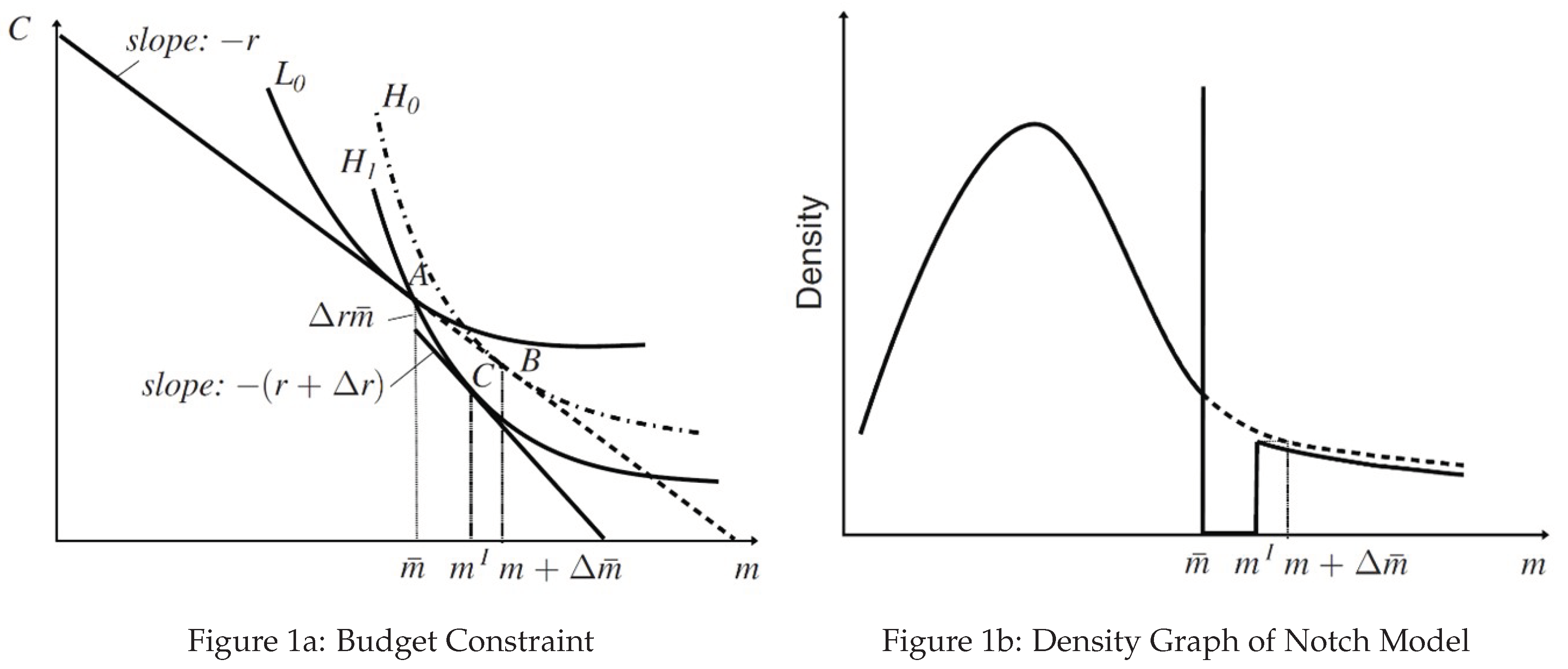
Figure 2.
Mean FICO Score across Years
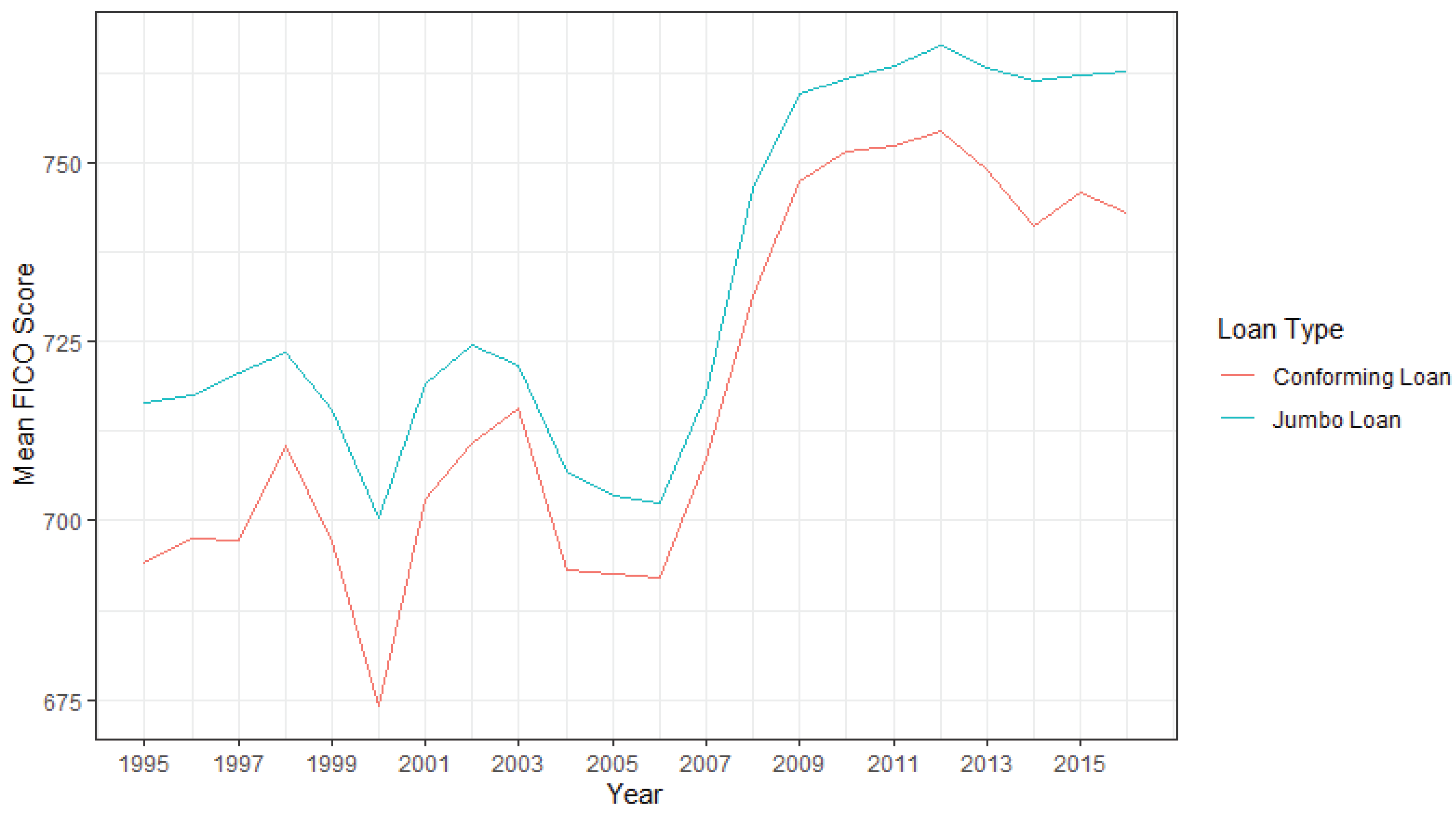
Figure 3.
Interest Rate of Conforming & Jumbo Loans
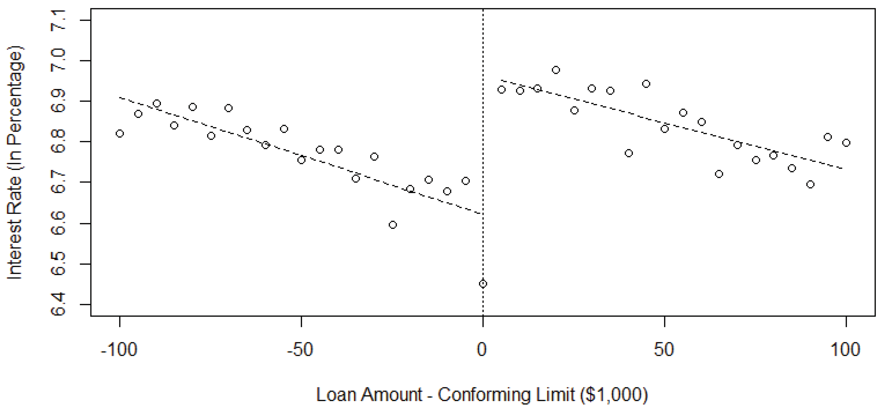
Figure 4.
Bunching Behavior Graph
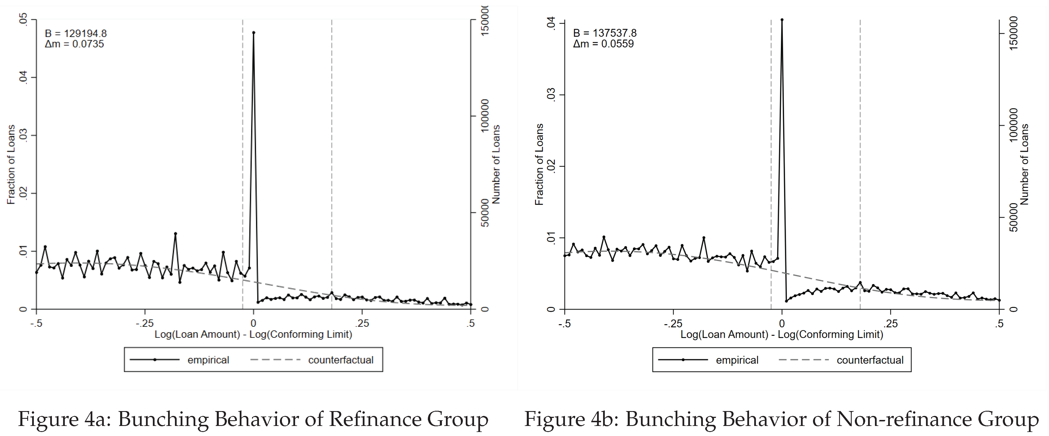
Figure 5.
FICO and Bunching
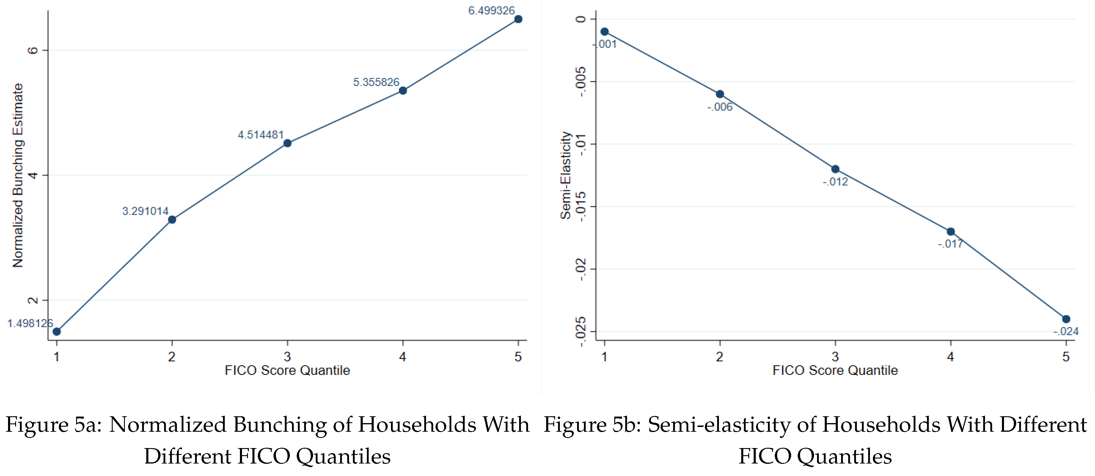
Table 2.
Refinance Group With & Without Liquidity Constraint
| With Liquidity Constraint | Without Liquidity Constraint | |
|---|---|---|
| (1) | (2) | |
| Bunched loans () | ||
| Behavioral response () | ||
| Excess mass () | ||
| Upper limit () | ||
Table 3.
Non-refinance Group With & Without Liquidity Constraint
| With Liquidity Constraint | Without Liquidity Constraint | |
|---|---|---|
| (1) | (2) | |
| Bunched loans () | ||
| Behavioral response () | ||
| Excess mass () | ||
| Upper limit () | ||
Disclaimer/Publisher’s Note: The statements, opinions and data contained in all publications are solely those of the individual author(s) and contributor(s) and not of MDPI and/or the editor(s). MDPI and/or the editor(s) disclaim responsibility for any injury to people or property resulting from any ideas, methods, instructions or products referred to in the content. |
© 2025 by the authors. Licensee MDPI, Basel, Switzerland. This article is an open access article distributed under the terms and conditions of the Creative Commons Attribution (CC BY) license (http://creativecommons.org/licenses/by/4.0/).
Copyright: This open access article is published under a Creative Commons CC BY 4.0 license, which permit the free download, distribution, and reuse, provided that the author and preprint are cited in any reuse.


