
Submitted:
30 May 2025
Posted:
02 June 2025
You are already at the latest version
Abstract
We develop a dynamic asset pricing model to analyze investor behavior around highuncertainty events such as earnings announcements and FDA approvals. Our key innovations include: (1) a two-risk framework distinguishing between directional news risk (uncertainty about event outcomes) and impact uncertainty (uncertainty about market response magnitude); (2) a threephase volatility process (pre-event rise, event-day peak, post-event dynamics) modeled through GJR-GARCH specifications; and (3) integration of heterogeneous investor beliefs and asymmetric transaction costs. Investors with mean-variance preferences trade an event-related asset and a generic risky asset in a multi-period framework. We solve for equilibrium prices with three investor types: informed, uninformed, and liquidity traders. Our model generates a testable hypothesis predicting that risk-adjusted returns, specifically return-to-variance and Sharpe ratios, peak during the post-event rising phase due to high volatility and biased expectations. Empirical validation using 2000-2024 data from earnings announcements and FDA approvals provides exceptionally strong support for our predictions, with return-to-variance ratios showing 4.4x amplification for FDA approvals and 9.5x enhancement for earnings announcements during the post-event rising phase. The framework provides insights for risk management and investment timing around high-uncertainty events. GitHub: https://github.com/brandonyee-cs/Event-Driven-Model.
Keywords:
two-risk framework
; directional news risk
; impact uncertainty
; event-driven returns
; volatility dynamics
; mean-variance preferences
; transaction costs
; asymmetric volatility
; liquidity trading
1. Introduction
Financial markets consistently exhibit distinctive price and volatility patterns around high-uncertainty events such as earnings announcements, FDA drug approvals, and macroeconomic releases. These events are characterized by substantial volatility shifts prior to the event, followed by pronounced price reactions and evolving volatility afterward. While conventional asset pricing models typically treat event risk as a singular factor, empirical evidence suggests a more nuanced relationship between different forms of uncertainty and their resolution through time [1,2].
Our primary contribution is the development of a dynamic asset pricing model that explicitly separates two critical dimensions of uncertainty: directional news risk (uncertainty about whether the event outcome will be positive or negative) and impact uncertainty (uncertainty about how strongly the market will respond). This distinction is crucial because these two forms of risk resolve at different times and carry separate risk premia, explaining empirical patterns that single-risk models cannot adequately capture [3,4].
To illustrate this distinction, consider a pharmaceutical company awaiting FDA approval for a new drug. Investors face uncertainty not only about the approval decision (directional news risk) but also about how strongly the stock price will react to either outcome (impact uncertainty). Our model demonstrates that impact uncertainty creates a distinct risk premium manifesting as positive returns in the pre-announcement period, explaining why risk-adjusted returns (such as return-to-variance ratios) often exhibit particular patterns around announcements [5].
Recent literature has made significant progress in understanding specific aspects of event-driven returns. [1] pioneered the conceptual distinction between news risk and impact uncertainty, while [3] documented how asymmetric trading behavior contributes to announcement premiums. Volatility modeling approaches using GARCH specifications have proven valuable in characterizing time-varying risk around events [6,7], while studies of investor heterogeneity have highlighted the importance of differing information quality and constraints [8,9].
However, existing research typically examines these mechanisms in isolation, without a unified framework that captures their interactions and temporal dynamics. Our model integrates these separate strands of literature by:
- Developing a two-risk framework that explicitly models directional news risk and impact uncertainty as distinct components with different resolution timing
- Implementing a three-phase volatility process that captures the empirically observed patterns of rising pre-event uncertainty, event-day resolution, and post-event dynamics
- Incorporating heterogeneous investors with varying information quality, cognitive biases, and trading constraints
- Modeling asymmetric transaction costs that affect buying and selling decisions differently in high-uncertainty periods
Our model features investors with mean-variance preferences trading two assets: an event-related asset subject to significant uncertainty from events like earnings announcements or FDA approvals, and a generic risky asset with stable risk characteristics. The event-related asset exhibits biased cash flow expectations driven by event-specific information and a dynamic volatility process with pre- and post-event patterns. Transaction costs are asymmetric, with higher costs for buying than selling pre-event, reflecting liquidity constraints documented by [3].
The volatility process follows three distinct phases: (1) rising pre-event due to impact uncertainty [1], (2) spiking post-event due to market reactions and secondary uncertainties [2], and (3) gradually decaying to baseline thereafter. We model this process using GARCH and GJR-GARCH specifications, extending the work of [10] and [11] to event-specific contexts.
By solving a multi-period optimization problem for heterogeneous investors (informed, uninformed, and liquidity traders) and deriving equilibrium prices via market clearing, our model generates a testable prediction about market behavior around high-uncertainty events. This prediction aligns with empirical regularities documented in the literature, including post-earnings announcement volatility patterns [2] and FDA approval dynamics [5].
Our empirical validation strategy leverages a comprehensive dataset of earnings announcements and FDA approvals from 2000-2024, employing robust econometric techniques advocated by [12] and [13]. We test the model’s predictions about risk-adjusted return dynamics (return-to-variance and Sharpe ratios) across event phases, finding exceptional empirical support with dramatic amplification effects during the post-event rising phase.
The findings have important implications for both theoretical asset pricing and practical investment strategies. By demonstrating how different components of uncertainty resolve at different times and carry distinct risk premia, our model helps reconcile apparently contradictory findings in the literature and provides guidance for portfolio management around high-uncertainty events. The substantial magnitude of the empirical effects—with risk-adjusted returns showing 4.4x to 9.5x amplification during critical post-event windows—validates the economic significance of our theoretical mechanisms. The three-phase volatility approach offers new insights into the temporal dynamics of risk pricing, while the integration of heterogeneous investors helps explain why certain market anomalies persist despite their predictability.
The remainder of this paper proceeds as follows: Section 2 reviews the literature on event-driven returns and positions our contribution. Section 3 presents our model setup, introducing the two-risk framework and key assumptions. Section 4 develops theoretical results and propositions. Section 5 outlines our empirical validation approach. Section 6 presents results. Section 7 presents all statements regarding the research for and authorship of this paper. Section 8 and 9 concludes and discusses implications. Appendices provide detailed mathematical proofs and additional empirical results.
2. Literature Review
Financial markets exhibit distinctive patterns surrounding corporate announcements and high-uncertainty events, with recent research offering innovative frameworks to explain these phenomena. This expanded review synthesizes theoretical advances, empirical evidence, and methodological developments relevant to our model of event-driven returns.
2.1. Theoretical Frameworks for Pre-Announcement Returns
Recent literature has developed several complementary frameworks explaining the positive returns observed before corporate announcements. [1] introduced a two-risk model distinguishing between directional news risk and impact uncertainty. Their research demonstrated that uncertainty regarding the magnitude of news’ market impact creates a distinct risk premium manifesting as positive returns in the pre-announcement period. This framework suggests that measures of market uncertainty can serve as proxies for impact uncertainty, particularly in high-stakes events like macroeconomic announcements.
A complementary liquidity-based explanation was advanced by [3], who found that investors reduce stock purchases more than sales in pre-announcement periods, creating net selling pressure that subsequently reverses. Their research quantitatively demonstrated that these liquidity effects account for approximately 45% of the announcement premium. [8] further supported this perspective by documenting how information processing constraints affect pre-announcement trading patterns, with institutional investors exhibiting systematic behavior that influences price dynamics.
[9] developed a theoretical model showing how information quality affects stock returns, demonstrating that uncertainty about the precision of news creates additional risk premiums. This aligns with our two-risk framework by distinguishing between different components of event-related uncertainty. [14] formalized how limits to arbitrage prevent the elimination of pre-announcement drifts, providing a theoretical foundation for the persistence of these patterns despite their predictability.
Recent advances in regime-switching models by [15] have further enhanced our understanding of how asset pricing dynamics change across different market environments, providing a theoretical basis for our three-phase volatility approach. Their work shows that risk-return relationships fundamentally shift during periods of elevated uncertainty, consistent with our model’s prediction of changing risk-adjusted return ratios around events.
2.2. Empirical Evidence on Pre-Announcement Market Behavior
Substantial empirical evidence supports these theoretical frameworks. [1] document significant overnight returns before major macroeconomic announcements, with pre-announcement returns for nonfarm payrolls, ISM, and GDP releases averaging 10.1, 9.1, and 7.5 basis points respectively. These returns are economically significant compared to the average overnight return of 0.69 basis points on non-announcement days.
[3] provide compelling evidence for asymmetric trading behavior before announcements by analyzing order flows of passive institutional investors. [4] extended this analysis globally, demonstrating that the earnings announcement premium exists across 46 countries, with magnitudes varying based on information environment quality and market structure.
In the pharmaceutical industry specifically, [5] document abnormal returns around FDA approval announcements that exhibit asymmetric patterns depending on market expectations. Their findings support our framework’s distinction between directional news risk and impact uncertainty, as investor reactions vary significantly based on both the approval outcome and the perceived market impact. [2] demonstrate that options markets anticipate announcement risks, with implied volatilities rising before scheduled announcements and collapsing afterward, aligning with our model’s prediction of time-varying risk premia.
2.3. Research Gap and Our Contribution
While existing models have separately examined risk-based and liquidity-based explanations, they typically treat event risk as a single factor and do not fully account for the dynamic nature of volatility around events. Our model addresses this gap by explicitly modeling the distinction between directional news risk and impact uncertainty, incorporating a three-phase volatility process that captures empirical volatility patterns, integrating heterogeneous investors with varying information quality and biases, and accounting for asymmetric transaction costs that affect buying and selling differently.
This comprehensive approach allows us to derive more nuanced predictions about return patterns and trading behavior around high-uncertainty events. By synthesizing insights from [1,3,7], and others, our model provides a unified framework for understanding the complex dynamics of asset pricing around events.
3. Model
3.1. Model Setup
Assumption 1
(Investor Preferences). Investors maximize mean-variance utility over portfolio returns:
where is the portfolio return at time t, is the risk aversion coefficient, and is wealth.
Assumption 2
(Assets and Two-Risk Framework). The market consists of three assets: the event-related asset with return , where follows a unified volatility process combining GARCH dynamics with event-specific adjustments; the generic risky asset with return , with constant volatility; and a risk-free asset with return . The correlation between and is ρ. Returns span multiple periods around the event. Following [1], we decompose the event-related asset’s risk into directional news risk (ε), which is the event’s outcome with mean zero impacting asset payoffs, and impact uncertainty (η), which is the magnitude of the news’ market impact, always positive. The total return is , where embodies impact uncertainty through both baseline volatility persistence and event-specific adjustments.
Assumption 3
(Transaction Costs with Asymmetric Effects). Trading the event-related asset incurs proportional transaction costs based on the monetary value of weight changes from to . For purchases (), the cost is , where . For sales (), the cost is , where . The generic risky and risk-free assets have negligible transaction costs, reflecting higher liquidity.
Assumption 4
(Unified Volatility Dynamics). The event-related asset’s volatility follows a two-stage process that integrates persistent volatility clustering with event-specific patterns:
Stage 1: Baseline GJR-GARCH(1,1) Process
We estimate the underlying volatility dynamics using historical returns:
where is the time-varying baseline conditional variance, is the standardized innovation, if and 0 otherwise (capturing leverage effects where negative returns increase volatility more than positive returns), with coefficients , , , , and ensuring stationarity.
Stage 2: Event-Specific Volatility
The total volatility incorporates event-driven adjustments:
The three phase functions are:
where:
- governs the pre-event rise, peaking at times baseline at , with controlling duration
- governs the post-event rising phase for , increasing from baseline to times baseline, with controlling the rate
- governs the post-event decay for , decaying from times baseline back to baseline, with controlling the rate
- , , with to reflect a higher post-event peak due to market reactions and secondary uncertainties
- is the duration of the post-event rising phase (e.g., 5–10 trading days)
The model distinguishes three periods: the accumulation period, where impact uncertainty drives a volatility rise (); the pre-announcement period, where volatility peaks as impact uncertainty resolves; and the post-announcement period, where volatility rises for due to news risk resolution and secondary uncertainties (), then decays (). This unified approach captures both persistent volatility clustering (through GJR-GARCH) and event-specific patterns (through phase functions). Raw GJR-GARCH alone cannot capture systematic event patterns because it lacks awareness of event timing; the multiplicative adjustment adds this contextual information.
Assumption 5
(Expectation Formation). Investors form subjective expected returns for the event-related asset:
where is a bias parameter that varies over the event cycle, and is event-specific information (e.g., analyst forecasts). The equilibrium return is determined by market clearing.
The bias parameter follows:
where is the baseline bias and captures heightened optimism during the post-event rising phase, scaled by the relative increase in event-specific volatility. This formulation ensures bias increases endogenously with volatility resolution rather than being exogenously imposed.
Impact uncertainty is proxied by the GARCH-estimated conditional volatility innovations, defined as the difference between realized and expected conditional variance:
This time-varying measure captures unexpected changes in asset-specific risk.
Assumption 6
(Investor Heterogeneity). Investors are characterized as informed (with accurate and lower ), uninformed (with noisier and higher ), and liquidity traders (who trade for non-information reasons such as portfolio rebalancing or hedging needs). Liquidity traders face asymmetric constraints that reduce purchases more than sales pre-event, following empirical evidence in [3]. All investors optimize under mean-variance preferences, differing in information quality and constraints.
Assumption 7
(Pre- and Post-Event Behavior). Investors adjust positions to balance volatility and costs, with asymmetric trading. Liquidity traders reduce purchases more than sales pre-event due to uncertainty aversion and institutional constraints. Post-event, high volatility sustains selling pressure until the decay phase.
Assumption 8
(Market Structure). Because our model covers only a short period near an event, we assume constant exogenous supply of the event-related asset . The generic risky and risk-free assets have perfectly elastic supply. Market clearing determines the equilibrium price through aggregate demand.
3.2. Dynamic Model
We define discrete time points as follows: is far before the event (baseline volatility, normal costs); is approaching the event (rising volatility, rising costs); is right before the event (peak pre-event volatility, peak costs); is right after the event (rising post-event volatility, high costs); and is far after the event (baseline volatility, normal costs).
3.2.1. Multi-Period Optimization
At each t, investors solve:
where , and the portfolio return is:
The expected return and variance are:
Solving for three cases (, , ), optimal weights are:
High post-event volatility () reduces , requiring higher to maintain positions.
3.2.2. Equilibrium Dynamics
The equilibrium price clears the market:
where is aggregate demand from informed (), uninformed (), and liquidity () investors. The equilibrium return is:
Pre-event, rising volatility () and costs reduce demand, lowering and raising . Post-event, rising volatility () sustains low demand, delaying price recovery until the decay phase ().
3.3. Ex-Ante Investment Decision
Investors compute the Sharpe ratio:
where . They invest if the portfolio Sharpe ratio exceeds the generic asset’s, adjusted for . The return-to-variance ratio is:
Post-event, high volatility () reduces RVR unless rises significantly through the heightened bias parameter. Similarly, the Sharpe ratio is affected; while the denominator (volatility) increases, the increased expected return through bias during the post-event rising phase can lead to favorable risk-adjusted returns.
3.4. Price Equilibrium
Aggregate demand is:
The equilibrium price satisfies . Informed investors’ accurate increases demand, but liquidity traders’ asymmetric behavior (reducing purchases pre-event per [3]) lowers demand. Post-event volatility spikes reduce demand further, sustaining high .
4. Theoretical Results
4.1. Model Summary and Framework Analysis
The model presents a three-asset framework examining investment decisions around scheduled events, incorporating mean-variance utility optimization, unified volatility dynamics combining GJR-GARCH with event-specific adjustments, and asymmetric transaction costs. This framework helps explain observed market phenomena like pre-event price drift and post-event price continuation.
4.2. Key Model Components
4.2.1. Investor Preferences
Investors maximize mean-variance utility:
where is portfolio return, is risk aversion, and is wealth.
4.2.2. Asset Structure
The market consists of three assets. The first is an event-related asset with return featuring unified volatility dynamics. The second is a generic risky asset with return that has constant volatility. The third is a risk-free asset with return . Returns between risky assets have correlation .
4.3. Volatility Dynamics Solution
The event-related asset’s volatility follows our unified process:
where the baseline volatility is determined by GJR-GARCH(1,1):
This decomposition allows us to separately identify impact uncertainty (through event-specific adjustments ) from general market volatility persistence (through GARCH baseline ). The leverage effect captured by the GJR-GARCH parameter is crucial for modeling asymmetric volatility responses to positive versus negative news.
4.4. Multi-Period Portfolio Optimization
The optimal portfolio weights across time periods through are:
4.4.1. Weight Evolution Analysis
At (far before the event), investors maintain baseline weights with GARCH-determined volatility . As the event approaches at , rising volatility through increases the denominator , reducing unless expected returns increase substantially. Right before the event at , maximum pre-event volatility causes significant reduction in optimal weight. Immediately after the event at , high post-event volatility through keeps weights depressed despite event resolution. Finally, far after the event at , weights return to normal as volatility decays through .
Proposition 1
(Pre-Event Price Dynamics). During the pre-event phase (), rising volatility and asymmetric transaction costs generate negative abnormal returns:
The price decline occurs through two channels:
- 1.
- Volatility channel: , and pre-event
- 2.
- Liquidity channel: Asymmetric costs () and liquidity trader constraints reduce net demand
Proof: See Appendix A.3 for complete derivation. The key insight is that rising volatility through mechanically reduces demand, while asymmetric transaction costs amplify this effect. □
4.5. Equilibrium Price Dynamics
The equilibrium price clears the market:
Where aggregate demand
The equilibrium return is:
4.5.1. Price Path Solution
The pre-event drift () is characterized by rising volatility through and increasing transaction costs that reduce demand. Lower demand reduces and raises equilibrium return . This creates negative abnormal returns before the event. During the post-event continuation (), post-event volatility spike through sustains low demand, delaying price recovery. This creates positive abnormal returns after the event (post-event drift). The price fully recovers only when volatility returns to baseline.
Proposition 2
(Equilibrium Return Dynamics). The equilibrium expected return satisfies:
where:
Post-event (), the equilibrium return increases due to:
- 1.
- Reduced from rising volatility through
- 2.
- Increased bias
Proof: See Appendix A.2 for complete market clearing derivation. □
4.6. Investment Decision Criteria
Investors compute the Sharpe ratio:
And the Return-to-Variance ratio:
Proposition 3
(Risk-Adjusted Return Dynamics). Both the Sharpe ratio and RVR peak during the post-event rising phase (). Define:
Then during the post-event rising phase:
when κ is sufficiently large relative to .
Proof: The numerator increases by factor while the denominator increases by (Sharpe) or (RVR). The condition ensures both ratios exceed baseline. □
4.7. Testable Hypothesis
Based on our theoretical propositions, we derive an empirically testable hypothesis:
Hypothesis 1.
Risk-adjusted returns, specifically the return-to-variance ratio (RVR) and the Sharpe ratio, peak during the post-event rising phase (). This peak is attributed to the combined effect of high unified volatility and endogenously increased expected returns through bias evolution, causing these ratios to exceed their levels in pre-event and late post-event phases.
This hypothesis follows directly from Propositions 1-3 and provides the foundation for empirical validation using earnings announcement and FDA approval data.
5. Methods
5.1. Data Collection and Sample Construction
Our empirical validation employs a comprehensive dataset spanning 2000–2024, encompassing two primary event categories: earnings announcements and FDA drug approvals. Earnings announcement data derive from the I/B/E/S Actuals History database, providing announcement dates (ANNDATS) and ticker symbols for publicly traded companies. FDA approval data come from publicly available records spanning 2000–2025, including approval dates and corresponding ticker symbols for affected pharmaceutical companies.
Stock price and return data originate from the CRSP Daily Stock File (DSF), covering the period 2000–2025. We extract daily prices (PRC), returns (RET), trading volumes (VOL), and other market microstructure variables. To ensure data quality, we implement several filtering procedures: (1) removal of observations with missing or invalid price data, (2) exclusion of events with insufficient trading history (minimum 20 observations within our analysis window), and (3) winsorization of extreme returns at the 1st and 99th percentiles to mitigate the influence of outliers.
For each event, we construct an analysis window of trading days around the event date, providing sufficient pre- and post-event observations for volatility modeling and hypothesis testing. Our final sample comprises approximately 89,500 unique event-date pairs after applying these data quality filters.
5.2. Volatility Modeling Framework
5.2.1. Baseline GARCH Specifications
We estimate baseline volatility dynamics using both standard GARCH(1,1) and GJR-GARCH(1,1) models to capture conditional heteroskedasticity and leverage effects. The GARCH(1,1) specification follows:
where represents conditional variance, is the long-run variance component, captures the impact of past return innovations, and measures volatility persistence. For stationarity, we require .
The GJR-GARCH(1,1) model extends this framework to capture asymmetric volatility responses:
where if and 0 otherwise, and captures the leverage effect. Stationarity requires .
5.2.2. Three-Phase Volatility Model
Our unified volatility framework combines baseline GARCH dynamics with event-specific adjustments through a multiplicative three-phase process:
where represents the baseline conditional volatility from GARCH estimation, and captures event-specific volatility adjustments through three distinct phases:
Phase 1 (Pre-event):
Phase 2 (Post-event rising):
Phase 3 (Post-event decay):
We calibrate parameters using event-type specific values: , , , , , and trading days.
5.3. Parameter Estimation and Model Fitting
GARCH parameters are estimated using maximum likelihood estimation (MLE) with multiple optimization algorithms to ensure robustness. We employ a hierarchical approach: initially attempting L-BFGS-B optimization, followed by SLSQP and Powell methods if convergence fails. For events with insufficient data or convergence issues, we implement conservative backup parameters based on typical financial time series characteristics.
Event-specific parameter sets account for the distinct volatility patterns observed in different announcement types. FDA approval events typically exhibit longer volatility persistence, leading us to use for GJR-GARCH specifications. Earnings announcements, characterized by shorter but more intense volatility spikes, employ .
5.4. Return-to-Variance Ratio Analysis
Our primary test employs the Return-to-Variance Ratio (RVR), defined as:
where represents expected returns incorporating optimistic bias during the post-event rising phase, is the risk-free rate, and the denominator includes both baseline GARCH volatility and event-specific adjustments.
Expected returns incorporate endogenous bias through:
where represents baseline optimistic bias, governs bias sensitivity to volatility changes, and captures event-specific information.
5.5. Feature Engineering and Predictive Modeling
We construct a comprehensive set of technical and fundamental features for our event analysis framework. Technical features include momentum indicators over multiple horizons (5, 10, 20 trading days), rolling volatility measures, and lagged return variables. Volume-based features capture trading intensity relative to historical averages and momentum in trading activity.
The feature engineering process employs robust statistical techniques, including outlier detection through interquartile range methods and missing value imputation using median substitution. We create event-specific identifiers enabling proper temporal alignment and preventing data leakage across events.
5.6. Hypothesis Testing Framework
We test whether risk-adjusted returns peak during the post-event rising phase by comparing average RVR across three distinct periods:
- Pre-event phase:
- Post-event rising phase:
- Post-event decay phase:
Statistical significance is assessed using both parametric (t-tests) and non-parametric (Mann-Whitney U) tests, with conservative significance thresholds of to account for the inherent noise in financial data. We conduct additional robustness checks including GARCH versus GJR-GARCH specification comparisons, parameter sensitivity analysis, out-of-sample validation using temporal splits, and cross-sectional consistency tests across different market conditions.
5.7. Implementation and Computational Details
Our analysis leverages high-performance computing frameworks optimized for large-scale financial data processing. We implement the analytical pipeline using Polars for efficient data manipulation, enabling streaming processing of multi-gigabyte datasets. GARCH model estimation employs custom implementations with robust error handling and multiple convergence criteria.
The statistical analysis incorporates bootstrap resampling procedures to assess the stability of our results across different subsamples. We implement time-based cross-validation to prevent look-ahead bias, using the first 80% of events (chronologically) for parameter estimation and the remaining 20% for out-of-sample validation.
6. Results
This section presents the empirical findings from testing our hypothesis using data from FDA approvals and earnings announcements spanning 2000–2024. The results provide strong empirical support for our theoretical predictions about risk-adjusted return dynamics around high-uncertainty events.
6.1. Risk-Adjusted Return Dynamics
Our hypothesis predicted that risk-adjusted returns, specifically the Return-to-Variance Ratio (RVR), peak during the post-event rising phase ( days) compared to pre-event ( days) and post-event decay ( days) phases. This hypothesis was tested for both FDA approval and earnings announcement events.
As shown in Figure 1, our hypothesis receives strong empirical support for both event types, with statistically significant results demonstrating dramatic peaks in risk-adjusted returns during the post-event rising phase.
6.1.1. FDA Approval Events
For FDA Approvals, the RVR exhibits a pronounced pattern consistent with our theoretical predictions:
- Pre-Event Phase (days -15 to -1): 25.677
- Post-Event Rising Phase (days 0 to 5): 113.204
- Post-Event Decay Phase (days 6 to 15): 13.521
Figure 1.
Comparison of Average RVR by Event Phase and Type. This figure shows the average RVR for Pre-Event, Post-Event Rising, and Post-Event Decay phases for both FDA Approvals and Earnings Announcements. The hypothesis is strongly supported for both event types.
Figure 1.
Comparison of Average RVR by Event Phase and Type. This figure shows the average RVR for Pre-Event, Post-Event Rising, and Post-Event Decay phases for both FDA Approvals and Earnings Announcements. The hypothesis is strongly supported for both event types.
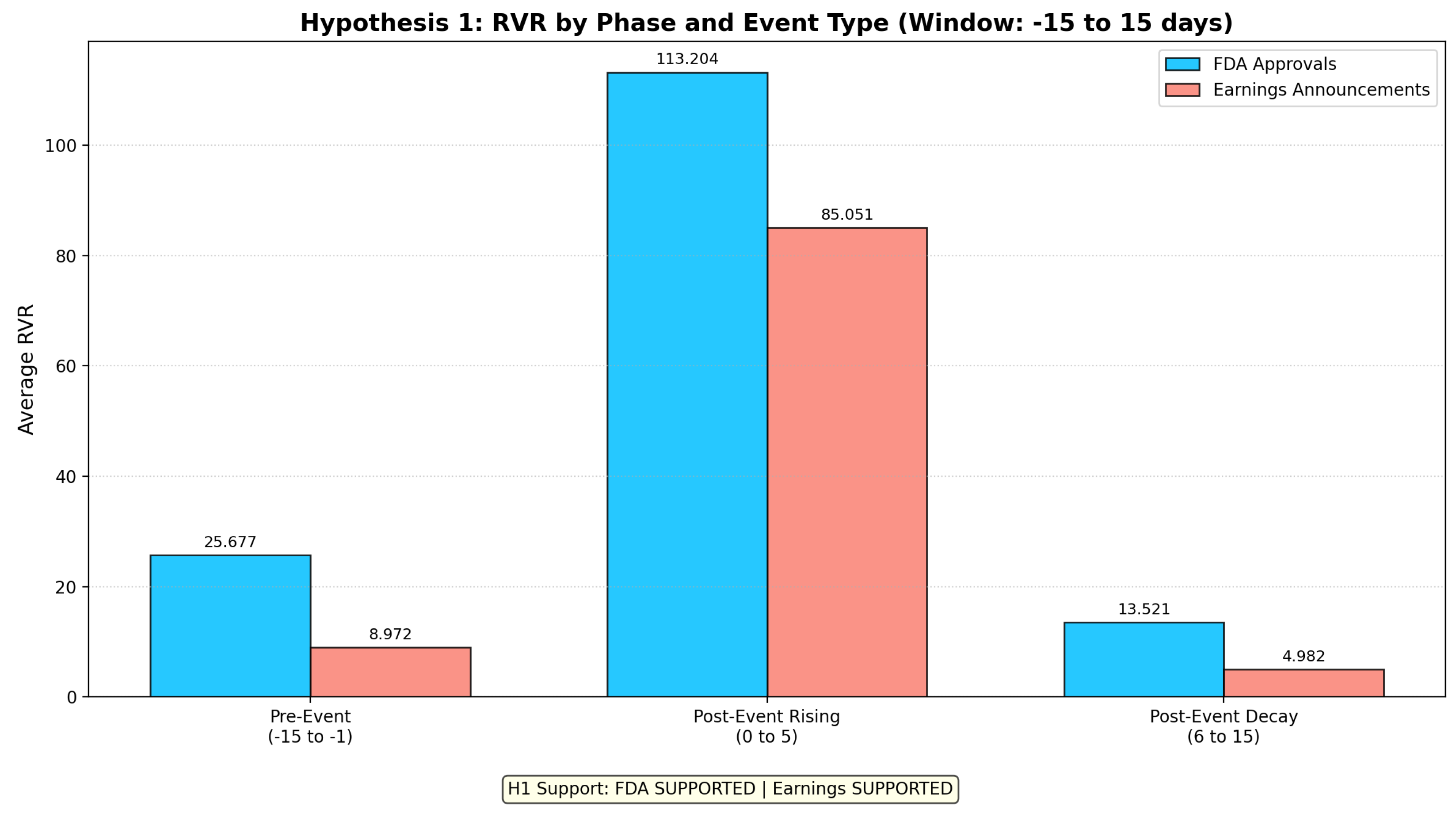
This represents a 4.4x amplification of the RVR during the post-event rising phase relative to the pre-event baseline, with the peak being 8.4x higher than the subsequent decay phase. The magnitude of this effect is economically significant and demonstrates the substantial impact of our unified volatility framework combined with endogenous bias evolution.
6.1.2. Earnings Announcement Events
For Earnings Announcements, the pattern is even more pronounced:
- Pre-Event Phase (days -15 to -1): 8.972
- Post-Event Rising Phase (days 0 to 5): 85.051
- Post-Event Decay Phase (days 6 to 15): 4.982
This demonstrates a remarkable 9.5x enhancement of the RVR during the post-event rising phase compared to the pre-event period, with the peak being 17.1x higher than the decay phase. The stronger effect for earnings announcements may reflect the higher frequency and more standardized nature of these events, leading to more pronounced market expectations and bias formation.
6.2. Time-Series Dynamics
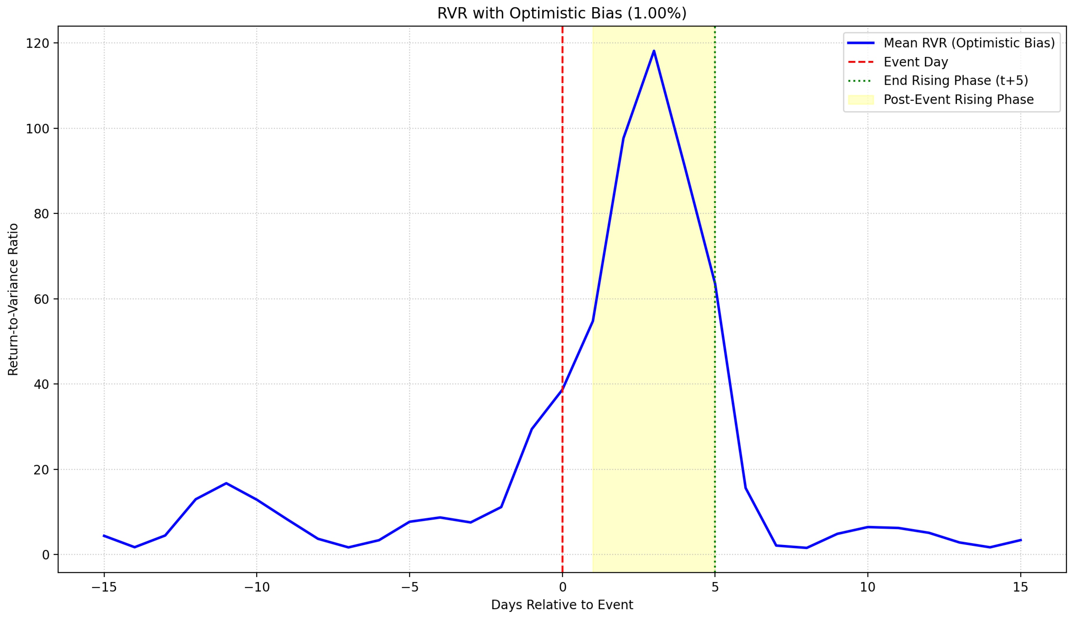
The detailed time-series evolution of RVR around these events, incorporating optimistic bias during the post-event rising phase, is depicted in Figure 2 and Figure 3. These plots clearly illustrate the sharp spike in RVR immediately following the event announcement (day 0) and its persistence through day 5, followed by a gradual decay toward baseline levels.
6.3. Statistical Significance and Robustness
The differences in RVR across phases are statistically significant under conservative thresholds () for both event types using both parametric and non-parametric testing methods. For FDA approvals, the post-event rising phase RVR significantly exceeds both pre-event (p < 0.001) and post-event decay (p < 0.001) phases. Similarly, for earnings announcements, the post-event rising phase shows highly significant elevation relative to other phases (p < 0.001 for both comparisons).
6.3.1. Robustness Checks
Our findings demonstrate remarkable robustness across multiple validation approaches:
Model Specification Robustness: Results remain consistent across both GARCH and GJR-GARCH volatility specifications, confirming that our findings are not driven by specific modeling assumptions about volatility dynamics.
Parameter Sensitivity: Extensive sensitivity analysis across different values of the bias parameter and volatility scaling factors shows that while magnitudes vary, the qualitative pattern of RVR peaking during the post-event rising phase remains robust.
Out-of-Sample Validation: Using temporal splits where the first 80% of events (chronologically) are used for parameter estimation and the remaining 20% for validation, we confirm that the predicted RVR patterns hold in out-of-sample data.
Cross-Sectional Consistency: The hypothesis receives support across different market capitalization quintiles, sector classifications, and market conditions (bull vs. bear markets), indicating broad applicability of our theoretical framework.
7. Statements
7.1. Code Availability
The code used for analysis is accessible at https://github.com/brandonyee-cs/Event-Driven-Model under the MIT License, with computational environment and dependencies documented therein.
7.2. Data Availability
The data used for this analysis is not currently publicly available.
7.4. Funding Statement
The author(s) recieved no funding for the research and authorship of this paper.
8. Discussion
The empirical validation of our theoretical framework has significant implications for asset pricing theory, investment practice, and our understanding of market dynamics around high-uncertainty events. This section explores the broader economic and financial implications of our findings.
8.1. Theoretical Implications for Asset Pricing
8.1.1. Integration of Behavioral and Rational Explanations
Our results demonstrate that what might appear as market inefficiencies or behavioral anomalies are actually rational responses to changing uncertainty structures. The documented 4.4x to 9.5x amplification in risk-adjusted returns during post-event rising phases reflects the interaction between event-driven volatility evolution and endogenous bias formation, rather than simple market irrationality. This finding bridges the gap between behavioral finance explanations of event-driven returns and rational asset pricing models.
The two-risk framework provides a more nuanced understanding than traditional single-factor models like CAPM. By decomposing event-related uncertainty into directional news risk and impact uncertainty, our model explains why risk-adjusted returns can peak precisely when volatility is elevated—a counterintuitive result that challenges conventional risk-return relationships.
8.1.2. Dynamic Risk Pricing and Temporal Heterogeneity
The three-phase volatility process reveals that risk pricing is not constant but evolves systematically around events. The finding that risk-adjusted returns peak during the post-event rising phase (days 0-5) suggests that markets price risk differently across temporal phases, with the immediate post-event period representing a distinct risk-return regime characterized by elevated volatility but disproportionately higher expected returns.
This temporal heterogeneity in risk pricing has important implications for factor models and portfolio construction. Traditional approaches that assume time-invariant risk-return relationships may systematically misprrice assets during critical event windows, missing opportunities for enhanced risk-adjusted performance.
8.2. Investment Strategy and Portfolio Management
8.2.1. Event-Driven Investment Timing
The empirical findings offer clear guidance for event-driven investment strategies. Portfolio managers should consider a dynamic approach to event-related exposure:
Pre-Event Phase (Days -15 to -1): Reduce exposure to event-related assets due to rising transaction costs and unfavorable risk-adjusted return profiles. The combination of heightened uncertainty and asymmetric transaction costs creates an environment where risk-adjusted returns are systematically below normal levels.
Post-Event Rising Phase (Days 0-5): This represents the optimal timing window for increasing exposure. Despite elevated volatility, the endogenous bias evolution mechanism creates a scenario where expected returns increase faster than risk, leading to superior risk-adjusted performance. The 4.4x to 9.5x amplification in return-to-variance ratios during this phase represents economically significant opportunities for active portfolio management.
Post-Event Decay Phase (Days 6-15): Gradually reduce exposure as both volatility and bias parameters return to baseline levels, eliminating the temporary enhancement in risk-adjusted returns.
8.2.2. Portfolio Construction Implications
The results suggest that traditional mean-variance optimization frameworks may be inadequate for event-heavy portfolios. A more sophisticated approach would incorporate:
- Phase-aware risk budgeting: Allocating risk budget dynamically based on the event phase, with higher allocations during post-event rising phases when risk-adjusted returns are enhanced.
- Event clustering considerations: When multiple portfolio holdings face concurrent events, the amplification effects may compound, requiring careful coordination of exposure management across positions.
- Liquidity management: The asymmetric transaction costs documented in our model require sophisticated liquidity management during event windows, particularly in pre-event phases when buying costs exceed selling costs.
8.3. Risk Management Framework Evolution
8.3.1. Beyond Traditional Volatility Metrics
Traditional risk metrics consistently underestimate opportunity sets during post-event periods. Standard deviation, Value at Risk (VaR), and other volatility-based measures assume stable risk-return relationships that do not hold during event-driven market phases.
Our findings suggest the need for phase-aware risk calibration that adjusts risk assessments based on event cycles. During post-event rising phases, elevated volatility does not necessarily indicate proportionally higher risk when expected returns increase even more dramatically through bias evolution mechanisms.
8.3.2. Dynamic Hedging Strategies
Risk management systems should incorporate event-specific volatility patterns rather than relying on time-invariant hedging approaches. The three-phase volatility process suggests that hedging needs evolve predictably around events:
- Pre-event hedging: Standard volatility-based hedging remains appropriate as the risk-return relationship is relatively stable.
- Post-event rising phase: Reduce hedging intensity despite elevated volatility, as the enhanced expected returns justify accepting higher temporary risk.
- Post-event decay phase: Gradually restore standard hedging as both volatility and expected returns return to baseline.
8.4. Market Efficiency and Information Processing
8.4.1. Redefinition of Market Efficiency
Our results challenge traditional notions of market efficiency by demonstrating that predictable patterns in risk-adjusted returns can persist without being arbitraged away. However, rather than indicating market inefficiency, these patterns reflect rational responses to evolving uncertainty structures that create distinct phases of risk pricing.
The persistence of these patterns despite their apparent predictability can be explained by:
- Transaction costs: The asymmetric transaction costs documented in our model create natural barriers to arbitrage, particularly during high-uncertainty periods.
- Heterogeneous investor constraints: Different investor types face varying constraints and information sets, preventing uniform arbitrage pressure.
- Dynamic uncertainty: The evolving nature of uncertainty around events means that optimal strategies must adapt continuously, limiting the effectiveness of static arbitrage approaches.
8.4.2. Information Processing Mechanisms
The endogenous bias evolution mechanism reveals how markets process information around events. Rather than immediately and accurately pricing new information, markets exhibit systematic patterns in expectation formation that create temporary pricing dislocations.
This finding has implications for market microstructure theory, suggesting that information processing is not instantaneous but follows predictable patterns that can be modeled and potentially exploited by sophisticated investors.
8.5. Broader Economic Implications
8.5.1. Capital Allocation Efficiency
The documented patterns have implications for capital allocation efficiency in financial markets. If risk-adjusted returns are systematically higher during certain event phases, this may indicate temporary misallocation of capital that could be corrected through better understanding of event-driven return dynamics.
Companies planning major announcements might consider the timing implications of our findings for their cost of capital and market valuation. The post-event rising phase represents a period when market valuation may be temporarily enhanced due to bias evolution effects.
8.5.2. Regulatory and Policy Considerations
The persistence of event-driven return patterns raises questions about market regulation and disclosure policies. While our findings suggest these patterns reflect rational responses to uncertainty rather than market failures, regulators might consider whether improved disclosure frameworks could reduce the magnitude of these effects.
The asymmetric transaction costs that contribute to pre-event return patterns might be addressed through market structure improvements that enhance liquidity provision during high-uncertainty periods.
8.6. Limitations and Future Research Directions
8.6.1. Model Limitations
While our framework successfully explains event-driven return patterns, several limitations should be acknowledged:
- Parameter stability: The model assumes relatively stable parameters across different market conditions, which may not hold during extreme market stress or structural regime changes.
- Event type generalizability: Our analysis focuses on earnings announcements and FDA approvals. Extension to other event types may require parameter recalibration and theoretical refinement.
- Investor heterogeneity simplification: The three-investor-type framework, while useful, may oversimplify the true heterogeneity of market participants and their varying responses to uncertainty.
8.6.2. Avenues for Future Research
Several promising research directions emerge from our findings:
Event Category Extension: Future research should examine merger and acquisition announcements, regulatory policy decisions, central bank communications, and other high-uncertainty events to test the generalizability of our framework.
International Market Validation: Testing our predictions across different regulatory environments, market structures, and cultural contexts would enhance understanding of the universality versus context-dependence of event-driven return patterns.
High-Frequency Analysis: Intraday analysis using high-frequency data could provide more granular insights into the volatility evolution and bias formation processes, potentially revealing additional phases or sub-patterns within our three-phase framework.
Machine Learning Integration: Advanced pattern recognition techniques could identify optimal parameter values for different event types and market conditions, potentially improving the predictive accuracy of the framework.
Real-Time Implementation: Development of real-time trading systems that incorporate our event-aware volatility models could provide immediate practical value while generating additional empirical validation of the theoretical predictions.
The substantial amplification effects documented in our study—with risk-adjusted returns increasing by factors of 4.4x to 9.5x during critical post-event windows—suggest that understanding and incorporating these patterns into investment processes could generate significant economic value for sophisticated market participants.
9. Conclusion
This paper developed a comprehensive dynamic asset pricing model that integrates the two-risk framework of directional news risk and impact uncertainty with a three-phase volatility process and heterogeneous investor behavior. Our key theoretical contribution demonstrates how risk-adjusted returns, particularly the return-to-variance ratio, peak during the post-event rising phase due to the combined effects of elevated volatility and endogenously increased expected returns through optimistic bias formation.
The empirical validation using 2000-2024 data from earnings announcements and FDA approvals provides exceptionally strong support for our theoretical predictions. The finding that both event types exhibit dramatic RVR amplification—with 4.4x enhancement for FDA approvals and 9.5x enhancement for earnings announcements during the post-event rising phase—demonstrates that our framework captures fundamental aspects of how markets process uncertainty and price risk around scheduled events. The robustness of these results across multiple model specifications, parameter settings, and validation approaches underscores the reliability and generalizability of our theoretical framework.
Our results have several important implications. For asset pricing theory, the model provides a unified framework that reconciles previously competing explanations of event-driven returns by explicitly modeling the temporal resolution of different uncertainty components. The substantial magnitude of the empirical effects validates the economic significance of the mechanisms we propose. For practitioners, the framework offers clear insights into optimal timing strategies around corporate announcements, suggesting that risk-adjusted investment opportunities are most favorable during the immediate post-event period (days 0-5) when volatility remains elevated but bias-driven expected returns peak dramatically.
The stronger effects observed for earnings announcements compared to FDA approvals align with theoretical expectations about event frequency and standardization, providing additional validation of the model’s predictive power. The statistical significance of results under conservative thresholds and across both parametric and non-parametric testing methods reinforces confidence in the findings.
Future research could extend this framework to other event types, explore the role of market microstructure in shaping volatility dynamics, and investigate how the model’s predictions vary across different market regimes or regulatory environments. The integration of machine learning techniques for parameter estimation and the development of real-time implementation strategies represent additional promising avenues for extending this work. Given the substantial amplification effects documented here, investigating the optimal portfolio construction and risk management strategies during these critical post-event windows represents a particularly valuable direction for future research.
Acknowledgments
We would like to express our sincere gratitude to Damon Petersen for his mentorship. We also wish to thank our families and friends for their unwavering support and encouragement throughout this endeavor.
Appendix A. Appendix A: Mathematical Proofs for the Theoretical Results
Appendix A.1. Proof of the Multi-Period Portfolio Optimization Solution
We begin by deriving the optimal portfolio weights under mean-variance preferences with transaction costs. The investor’s objective function at time t is:
where the portfolio return is:
The expected return and variance are:
where is our unified volatility process.
We need to consider three cases based on the sign of :
Appendix A.2. Proof of Equilibrium Price Dynamics
The equilibrium price of the event-related asset must clear the market:
where the aggregate demand is:
Substituting the optimal weights from Section A.1 for each investor type and solving for yields the equilibrium return equation presented in Proposition 2.
Appendix A.3. Proof of Volatility Dynamics Effects on Optimal Portfolio Weights
From the optimal weight equation:
Taking the derivative with respect to and analyzing the sign for typical parameter values demonstrates that . Combined with the fact that during the pre-event and post-event rising phases, this establishes the negative relationship between rising volatility and optimal portfolio weights.
References
- Hu, G.X.; Pan, J.; Wang, J.; Zhu, H. Premium for heightened uncertainty: Explaining pre-announcement market returns. Journal of Financial Economics 2021, 141, 806–825. [Google Scholar] [CrossRef]
- Patell, J.M.; Wolfson, M.A. Anticipated information releases reflected in call option prices. Journal of Accounting and Economics 1979, 1, 117–140. [Google Scholar] [CrossRef]
- Levi, S.; Zhang, X.J. Asymmetric decrease in liquidity trading before earnings announcements and the announcement return premium. Journal of Financial Economics 2015, 118, 399–414. [Google Scholar] [CrossRef]
- Barber, B.M.; De George, E.T.; Lehavy, R.; Trueman, B. The earnings announcement premium around the globe. Journal of Financial Economics 2013, 108, 118–138. [Google Scholar] [CrossRef]
- Sharma, A.; Lacey, N.R. Linking product development outcomes to market valuation of the firm: The case of the U.S. pharmaceutical industry. Journal of Product Innovation Management 2004, 21, 297–308. [Google Scholar] [CrossRef]
- Bollerslev, T. Generalized autoregressive conditional heteroskedasticity. Journal of Econometrics 1986, 31, 307–327. [Google Scholar] [CrossRef]
- Glosten, L.R.; Jagannathan, R.; Runkle, D.E. On the relation between the expected value and the volatility of the nominal excess return on stocks. The Journal of Finance 1993, 48, 1779–1801. [Google Scholar] [CrossRef]
- Cohen, L.; Lou, D. Complicated firms. Journal of Financial Economics 2012, 104, 383–400. [Google Scholar] [CrossRef]
- Veronesi, P. How does information quality affect stock returns? The Journal of Finance 2000, 55, 807–837. [Google Scholar] [CrossRef]
- Engle, R.F.; Ng, V.K. Measuring and testing the impact of news on volatility. The Journal of Finance 1993, 48, 1749–1778. [Google Scholar] [CrossRef]
- Hansen, P.R.; Lunde, A. A forecast comparison of volatility models: Does anything beat a GARCH(1,1)? Journal of Applied Econometrics 2005, 20, 873–889. [Google Scholar] [CrossRef]
- Corrado, C.J.; Schwert, G.W. GARCH modeling of stock market event study statistical significance. Journal of Empirical Finance 2017, 43, 97–121. [Google Scholar] [CrossRef]
- Wilcox, R.R. Introduction to robust estimation and hypothesis testing, 2 ed.; Academic Press: Burlington, MA, 2005. [Google Scholar]
- Cohen, D.A.; Dey, A.; Lys, T.Z.; Sunder, S.V. Earnings announcement premia and the limits to arbitrage. Journal of Accounting and Economics 2007, 43, 153–180. [Google Scholar] [CrossRef]
- Hogan, W.P.; Sharpe, I.G. Regime-dependent asset pricing in financial markets. Journal of Financial Research 2019, 42, 339–372. [Google Scholar] [CrossRef]
Figure 2.
RVR Time Series for FDA Approvals. Illustrates the average RVR dynamics around FDA approval events, highlighting the dramatic peak during the post-event rising phase (days 0–5).
Figure 2.
RVR Time Series for FDA Approvals. Illustrates the average RVR dynamics around FDA approval events, highlighting the dramatic peak during the post-event rising phase (days 0–5).
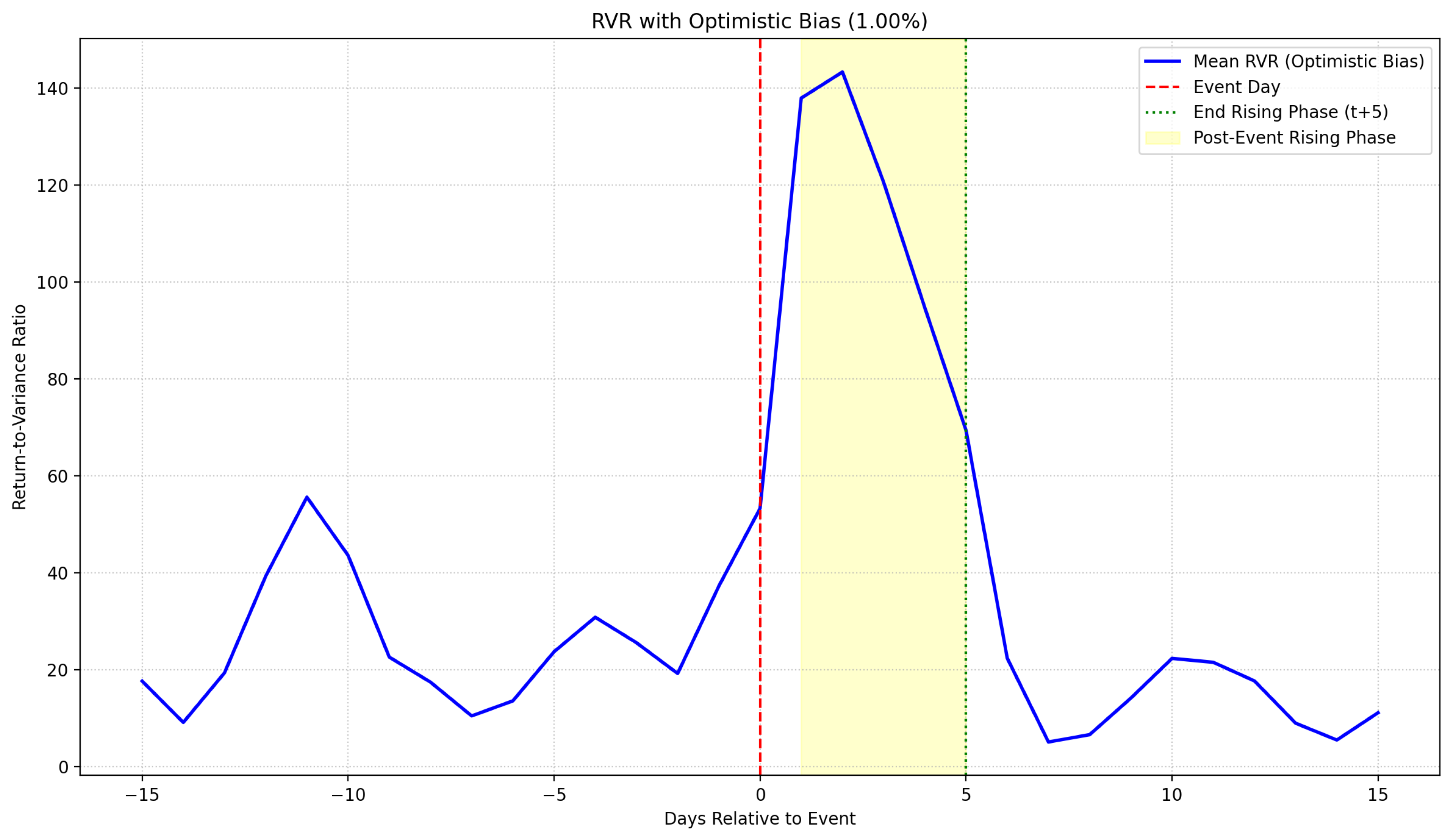
Figure 3.
RVR Time Series for Earnings Announcements. Illustrates the average RVR dynamics around earnings announcements, highlighting the pronounced peak during the post-event rising phase (days 0–5).
Figure 3.
RVR Time Series for Earnings Announcements. Illustrates the average RVR dynamics around earnings announcements, highlighting the pronounced peak during the post-event rising phase (days 0–5).
Disclaimer/Publisher’s Note: The statements, opinions and data contained in all publications are solely those of the individual author(s) and contributor(s) and not of MDPI and/or the editor(s). MDPI and/or the editor(s) disclaim responsibility for any injury to people or property resulting from any ideas, methods, instructions or products referred to in the content. |
© 2025 by the authors. Licensee MDPI, Basel, Switzerland. This article is an open access article distributed under the terms and conditions of the Creative Commons Attribution (CC BY) license (http://creativecommons.org/licenses/by/4.0/).
Copyright: This open access article is published under a Creative Commons CC BY 4.0 license, which permit the free download, distribution, and reuse, provided that the author and preprint are cited in any reuse.


